Submitted:
09 February 2024
Posted:
12 February 2024
Read the latest preprint version here
Abstract
We propose a neural-network-based watermarking method that introduces the quantized activation function that approximates the quantization of JPEG compression. Many neural network-based watermarking methods have been proposed. Conventional methods have acquired robustness against various attacks by introducing an attack simulation layer between the embedding network and the extraction network. The quantization process of JPEG compression was replaced by the noise addition process in the attack layer of the conventional methods. In this paper, we propose a quantized activation function that can simulate the JPEG quantization standard as it is in order to improve the robustness against the JPEG compression. Our quantized activation function consists of several hyperbolic tangent functions and is applied as an activation function for neural networks. Our network was introduced in the attack layer of Ahmadi et al.’s to compare it with their method. That is, the embedding and extraction networks had the same structure. We compared the usual JPEG compressed images and the images applying the quantized activation function. The results showed that a network with quantized activation functions can approximate JPEG compression with high accuracy. We also compared the bit error rate (BER) of estimated watermarks generated by our network with those generated by Ahmadi et al.’s. We found that our network was able to produce estimated watermarks with lower BERs than those of the method of Ahmadi et al.. Therefore, our network outperformed the conventional method with respect to image quality and BER.
Keywords:
Watermarking method
; Neural network
; Activation function
; JPEG compression
1. Introduction
People are now easily able to upload photos and illustrations to the Internet, owing to smartphones and personal computers. To protect content creators, we need to prevent unauthorized copying and other abuses because digital content is not degraded by copying or transmissions. Digital watermarking is effective against such unauthorized use.
In digital watermarking, secret information is embedded in digital content by making slight changes to the content. In the case of an image, the image in which the information is embedded is called a stego-image, and the embedded information is called a digital watermark. There are two types of digital watermarking: blind and non-blind. The blind method does not require the original image to extract the watermark from the stego-image. However, the non-blind method requires the original image when extracting a watermark from a stego-image. Therefore, the blind method is more practical. In addition, because stego-images may be attacked by various kinds of image processing, watermarking methods must have the ability to extract watermarks from degraded stego-images. Two types of attacks on stego images can occur: geometric attacks such as rotation, scaling, and cropping and non-geometric attacks such as noise addition and JPEG compression.
Neural-network-based methods have been proposed, ones that learn from embedding to extraction processes in an end-to-end manner [1,2,3,4]. Zhu et al.’s [1] method has an attack layer that simulates attacks such as Gaussian blurring, per-pixel dropout, cropping, and JPEG compression on images during training. Here, the implementation of JPEG compression is approximated by JPEG-Mask, which sets the high-frequency components of the discrete cosine transform (DCT) coefficients to zero, and JPEG-Drop, which uses progressive dropout to eliminate the high-frequency components of the DCT coefficients. Therefore, this implementation does not meet the standard for quantization in the JPEG compression process. Hamamoto and Kawamura’s method [3] also introduces a layer of additive white Gaussian noise as an attack layer to improve robustness against JPEG compression. Moreover, Ahmadi et al. [4] proposed attack layers implementing salt-and-pepper noise, Gaussian noise, JPEG compression, and mean smoothing filters. The quantization of the JPEG compression is approximated by adding uniform noise. As described, the quantization process has been replaced by the process of adding noise, and the quantization process as per the JPEG standard has not been introduced.
In this paper, we propose a quantized activation function that can simulate quantization of JPEG compression according to a standard. We apply this function to the attack layer of the method of Ahmadi et al. [4]. The robustness against the JPEG compression is expected to be improved using a standard-based function. The effectiveness of our method was evaluated by comparing JPEG compressed images with images in which the quantized activation function was applied. The image quality of the stego-image was also evaluated.
This paper is organized as follows. In Section 2, we present the details of the quantization process of JPEG compression and related research. In Section 3, we define the quantized activation function and describe the structure of the proposed network. In Section 4, we show the effectiveness of the function and demonstrate the performance of our network in computer simulations. We conclude in Section 5.
2. Related works
2.1. Quantization of JPEG compression
JPEG compression is a lossy compression that reduces the amount of information in an image to reduce the file size. In this kind of compression, an image is divided into -pixel blocks. Then, in each block, the processes of the DCT, quantization, and entropy coding are sequentially performed. In JPEG compression, the process of reducing the amount of information is the quantization process of the DCT coefficients. We focus on the quantization of the DCT coefficients of the luminance component in an image because the watermark is embedded in these coefficients of the image.
Figure 1 shows the quantization process in JPEG compression for DCT coefficients. The process consists of three steps: 1) creation of the quantization table , 2) the quantization process, and 3) the dequantization process.
2.1.1. Creation of the quantization table
During the quantization process, the DCT coefficients are quantized based on a default basic table or a self-defined basic table. The default basic table is defined as
The quantization table is then determined using the quality factor (Q) and the basic table . The quantization table for the quantization level Q at coordinates is defined as
where is the floor function and where is the component of the basic table . Also, the scaling factor is given by
2.1.2. Quantization process
The quantization process is performed using the quantization table . Let be the quantized data, and let be the DCT coefficients in an -pixel block. The quantization process is performed as
where is given by
2.1.3. Dequantization process
Let be the quantized DCT coefficients; then, the dequantization process is performed as
2.2. Implementation of quantization in related works
As mentioned in 1 introduction, the quantization process in existing methods is implemented by adding noise at the attack layer. In Ahmadi et al. [4], the quantization process is approximated using the quantization table and uniform noise . Let represent the DCT coefficients of an -pixel block of a stego image, and the quantized DCT coefficients are given as
In their method, the quantization process is equivalent to adding a uniform noise proportional to the quantization table .
3. Proposed method
We propose an attack layer that implements JPEG quantization using a quantized activation function (QAF). To demonstrate the effectiveness of the QAF, we compared it with the method of Ahmadi et al. (ReDMark) [4] using the same model as that in ReDMark for the watermark embedding and extraction networks.
3.1. Quantized activation function
We propose a quantized activation function for neural networks to implement the quantization process of the JPEG compression according to the standard. The QAF consists of n hyperbolic tangent functions tanh and is defined as
where is the value of the quantization table when the quantization level is Q. Also, is the slope of the hyperbolic tangent function. Figure 2 shows when the slope is 1 and when the value of the quantization table is 16.
3.2. ReDMark
Figure 3 shows the overall structure of ReDMark [4], which consists of an embedding layer, an extraction layer, and an attack layer. The h and w are the height and width of the 2D watermark, and H and W are the height and width of the original and stego images. The images are divided into -pixel blocks, where as it is in ReDMark.
In ReDMark [4], normalization and reshaping are performed on the input image in preprocessing. For the input image , the normalized image is given by
Reshape is an operation that divides an image into -pixel blocks and transforms them into a 3D tensor representation. The image size is assumed to satisfy . The reshaped image is represented by a 3-dimensional tensor of . This image is called the image tensor of size . If necessary, the tensor is inverse transformed back to its original dimension.
3.3. Embedding network
The embedding network, as shown in Figure 4, consists of three layers: convolution, circular convolution, and transform. The transform layer can perform lossless linear transforms using convolutional layers, e.g., the DCT, wavelet transform, and Hadamard transform. In our method, the DCT is selected as the transform layer as it is in ReDMark. The circular convolution layer extends the input to make it cyclic before the convolution is performed. Figure 5 shows an example of applying a circular convolution layer with a filter when the input is pixels. When a circular convolution layer is used, the dimension of the output after convolution is the same as the dimension of the input.
In the embedding network, the convolution and circular convolution layers use and filters, respectively, and both have 64 filters. In each layer, an exponential linear unit (ELU) activation function is used. The output of the embedding layer is obtained by summing the output of the transform layer performing the inverse DCT (IDCT) (for the IDCT layer) with the input image tensor of size and then by performing the inverse process of reshaping. Here, the output of the IDCT layer can be adjusted by the embedding intensity . The intensity is fixed as during training and can be changed during an evaluation.
3.4. Extraction network
The extraction network consists of a convolution layer, a circular convolution layer, and a transform layer, as shown in Figure 6. The transform layer of the extraction network also performs the DCT. The filter sizes of the convolutional and circular convolutional layers are and , respectively. The number of filters is 64 for the fourth layer and 1 for the fifth layer. The activation function up to the fourth layer is ELU [14], and a sigmoid function is used in the fifth layer. Let be the output of the extraction network, and the estimated watermark is given by
3.5. Attack layer
Various attacks can be simulated in the attack layer. In the attack layer of ReDMark, three attack layers are used depending on the type of attack: a GT-Net (a Gaussian-trained network), a JT-Net (a JPEG-trained network), and a MT-Net (a multi-attack-trained network). Because the JT-Net was trained to simulate the JPEG compression, it is compared with our network. The proposed attack layer consists of three sub-layers: a DCT layer, a layer introducing QAF (a QAF layer), and an IDCT layer. Note that in our network, the DCT coefficients are quantized as in the JPEG compression. Figure 7 shows the structure of the network. The embedding and extraction layers have the same structure as that of ReDMark [4]. The output of the DCT layer is processed by the QAF (9) at the QAF layer. The output of this layer is calculated by
Note that the quantization table is divided by 255 because it is normalized by (10). The quantization table values in (12) are determined according to because the quantization table values are different for each of the coordinates of the DCT coefficients. The coordinates are defined by
The attack layer [4] in ReDMark performs noise addition to the coefficients, while the one in our network performs the quantization with the QAF.
3.6. Training method
The embedding and extraction networks are trained in the same way as they were in ReDMark [4], respectively. The loss function of the embedding network is defined as
where is the original image given as a teacher and where is the output of the embedding network. and are the mean of and , respectively. and are the variances of each image, and is the covariance between the two images. Let and be constants, and let . Because the output of the embedding network takes a real number, the stego-image is obtained by converting it back to 256 levels of the pixel value. That is, it is given by
The loss function of the extraction network is defined as
where is the watermark used as a teacher for the extraction network. is the output of the sigmoid function of the extraction network. That is, it takes a value between 0 and 1. The total loss function L of our network is defined as
where the parameter determines the balance between the two loss functions. The embedding and extraction network are trained by the back propagation [7] using stochastic gradient descent (SGD) as the optimization method.
4. Computer Simulation
4.1. Evaluation of the QAF
First, we tested our method using a computer simulation in which the QAF could approximate the quantization process of JPEG compression. Because the DCT and quantization were applied to -pixel blocks in the JPEG compression, the QAF was also applied to -pixel blocks. Three images of pixels as shown in Figure 8 were selected from the dataset provided by the University of Granada [11]. Each image was normalized by (10) and was divided into -pixel blocks. The DCT was performed on each block. Let be the DCT coefficients of the -th block. The QAF was applied to the -th block as
where the quantization level of the JPEG compression was set to . The parameters of the QAF in (9) were set as gradient and the number of the hyperbolic tangent functions . For all the QAF-applied blocks, an IDCT was performed, and the luminance values were inversely normalized using (15). Next, all blocks were combined. The combined image was converted back to the original image size. Then, the QAF-applied image was given by
In general, the peak signal to noise ratio (PSNR) of an evaluated image against a reference image is defined by
where
The accuracy of the QAF can be measured by the PSNR of a QAF-applied image against a JPEG-compressed image, that is, , where is the JPEG-compressed image. Note that the PSNR was measured in the JPEG-compressed image, not the original image, to see the difference with the JPEG-compressed image. Figure 9 shows the three QAF-applied images and their PSNRs. The PSNRs were (a) , (b) , and (c) , all of which were sufficiently high. Thus, we found that the QAF adequately represents the quantization of the JPEG compression.
4.2. Evaluation of the proposed attack layer
We compared the JT-Net in the ReDMark and the proposed attack layer based on the image quality of stego-images and the BER of watermarks extracted from stego-images after the JPEG compression.
4.2.1. Experimental conditions
The training and test images were selected as they were in ReDMark [4]. The training images were 50,000 -pixel images from CIFAR10 (). An -bit watermark was embedded, where . The watermark was randomly generated. In the parameters used for training, the block height and width sizes were set to and , respectively. The parameter of the loss function (17) was set to , the number of learning epochs was set to 100, and the mini-batch size was set to 32. For the parameters of SGD, the training rate was set to , and the moment was set to . The quantization level for the JPEG compression was set to , and the quantization table was used. For training the proposed attack layer, the gradient of the QAF (9) was set to , and the number of the hyperbolic tangent functions was set to . The embedding, attack, and extraction layers were all connected, and the network was trained using the training images and watermarks. Here, the embedding intensity and quantization level were fixed at and , respectively.
For testing, 49 images of pixels from the University of Granada were used. These images were divided into pixel subimages, and the embedding process was performed on each of them. The 256 subimages were given to the network as test images. Meanwhile, a bit watermark was randomly generated. One watermark was embedded four times in one image. That is, the watermark was divided into -bit subwatermarks, and finally each subwatermark was embedded in one subimage. An estimated watermark was determined by bit-by-bit majority voting because the same watermark was embedded four times in one image.
The attack layer was not used during testing. The test images and the watermarks were used to output stego-images in the embedding network. Here, the embedding intensity was set to values from to . The stego-images were JPEG compressed at quantization levels . The compressed stego-images were input to the extraction network, and the estimated watermarks were output. These networks were trained 10 times with different initial values for the comparison of our network with the JT-Net on image quality and BER. The mean and standard deviation of structural similarity index measures (SSIMs), PSNRs, and BERs were calculated.
4.2.2. Evaluation of the image quality
The image quality of the stego-images obtained from the JT-Net and our network was evaluated using the SSIMs and PSNRs. The image quality of the stego-image against the original image can be expressed as and by (14) and (20). Figure 10 shows the SSIM and PSNR. The horizontal and vertical axes represent the embedding intensity and SSIM or PSNR, respectively. The error bars represent the standard deviation of the SSIMs and PSNRs. Embedding the watermark strongly causes degradation in the image quality. Therefore, the SSIM and PSNR decreased as the intensity increased. The image quality of our network was higher than that of the JT-Net. In other words, our network can reduce the degradation of image quality even with the same embedding intensity.
4.2.3. Evaluation of the BER
The robustness of our network against the JPEG compression was evaluated. The estimated watermark obtained by (11) was evaluated by using the BER. The BER of the estimated watermark can be defined by
where is the original watermark, and ⊕ represents the exclusive OR.
First, we compared the robustness of our network with that of the JT-Net using the same embedding intensity . Figure 11 shows the BER of the estimated watermark for the embedding intensity . The horizontal and vertical axes represent the intensity and BER, respectively. The solid and dashed lines were the results of our network and the JT-Net for various compression levels Q, respectively. When the watermark was strongly embedded, it was extracted correctly. Therefore, the BER decreased as the intensity increased. The lowest BER was obtained when . At compression level , the BER of the proposed network was lower than that of the JT-Net. Also, at , they had almost the same BER. Furthermore, at , the BER of our network was higher than that of the JT-Net. In practical use, is normally used, so our network was demonstrated to be effective.
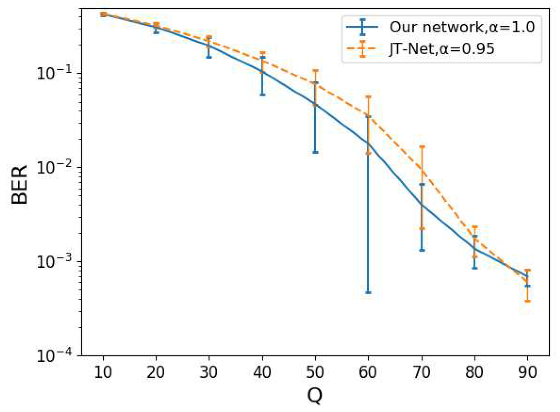
Even with the same embedding intensity, the image quality of our network differs from that of the JT-Net. Therefore, we next adjusted the embedding intensity so that the PSNR of both networks was almost the same, and we compared the BERs of both networks under this condition. Figure 12 is the BER for the compression level Q. The error bars are the standard deviation of the BERs. The intensity was chosen as part of our evaluation of the robustness against the JPEG compression so that the PSNR obtained from both networks was almost the same. The intensity for the JT-Net and for our network was set to (PSNR=) and (PSNR=), respectively. The BER of the estimated watermark for our network was lower than that for the JT-Net. Thus, we can say that our network can generate watermarks with fewer errors under the given PSNR.
5. Conclusion
The JT-Net in ReDMark [4] is a network that simulates JPEG compression. This network substituted the quantization process with a process that adds noise proportional to the value of the quantization table. In this paper, we proposed the quantized activation function (QAF), which can approximate the quantization process of the JPEG compression according to the standard. By approximating the quantization of the JPEG compression using the QAF, we expected to improve the robustness against the JPEG compression. The results of computer simulations showed that the QAF represented quantization with sufficient accuracy. Also, we found that the network trained with the QAF was more robust against the JPEG compression than those trained with the JT-Net. Because the embedding and extraction networks were more robust against the JPEG compression when trained with the QAF, we conclude that our method is more suitable for simulating JPEG compression than conventional methods applying additive noise.
Author Contributions
Conceptualization, M.K. ; methodology, M.K. and S.Y.; software, S.Y.; investigation, S.Y.; resources, M.K.; data curation, M.K. and S.Y.; writing—original draft preparation, S.Y.; writing—review and editing, M.K.; visualization, S.Y.; supervision, M.K.; project administration, M.K.; funding acquisition, M.K. All authors have read and agreed to the published version of the manuscript.
Funding
This work was supported by JSPS KAKENHI Grant Number 20K11973. The computations were performed using the supercomputer facilities at the Research Institute for Information Technology of Kyushu University.
Data Availability Statement
Publicly available datasets were analyzed in this study. This data can be found here: CIFAR-10 dataset https://www.cs.toronto.edu/ kriz/cifar.html and Computer Vision Group. University of Granada https://ccia.ugr.es/cvg/CG/base.htm
Acknowledgments
This work was supported by JSPS KAKENHI Grant Number 20K11973. The computations were performed using the supercomputer facilities at the Research Institute for Information Technology of Kyushu University.
Conflicts of Interest
The funders had no role in the design of the study; in the collection, analyses, or interpretation of data; in the writing of the manuscript; in the decision to publish the results.
References
- J. Zhu, R. Kaplan, J. Johnson, L. Fei-Fei, “HiDDeN: Hiding Data With Deep Networks,” European Conference on Computer Vision, 2018.
- I. Hamamoto, M. Kawamura, “Image watermarking technique using embedder and extractor neural networks,” IEICE transactions on Information and Systems, vol. E102-D, no. 1, pp. 19–30, 2019. [CrossRef]
- I. Hamamoto, M. Kawamura, “Neural Watermarking Method Including an Attack Simulator against Rotation and Compression Attacks,” IEICE transactions on Information and Systems, vol. E103-D, no. 1, pp. 33–41, 2020. [CrossRef]
- M. Ahmadi, A. Norouzi, S. M. Reza Soroushmehr, N. Karimi, K. Najarian, S. Samavi, A. Emami, “Redmark: Framework for residual diffusion watermarking based on deep networks,” Expert Systems with Applications, vol. 146, 2020. [CrossRef]
- Independent JPEG Group, http://www.ijg.org/, (Accessed 2023-05-21).
- G. E. Hinton, R. R. Salakhutdinov, “Reducing the Dimensionality of Data with Neural Networks,” Science, vol. 313, pp. 504–507, 2006. [CrossRef]
- D. E. Rumelhart, G. E. Hinton, R. J. Williams, “Learning representations by back-propagating errors,” Nature, vol. 323, no. 6, pp. 533–536, 1986. [CrossRef]
- D. P. Kingma, J. L. Ba, “Adam: A method for stochastic optimization,” Proceedings of 3rd international conference on learning representations, 2015.
- V. Nair, G. E. Hinton, “Rectified linear units improve restricted boltzmann machines,” Proceedings of the 27th international conference on machine learning, pp. 807–814, 2010.
- K. He, X. Zhang, S. Ren, J. Sun, “Delving deep into rectifiers: Surpassing human-level performance on imagenet classification,” Proceedings of the IEEE international conference on computer vision, pp. 1026–1034, 2015.
- Computer Vision Group at the University of Granada, Dataset of standard 512 × 512 grayscale test images, http://decsai.ugr.es/cvg/CG/base.htm, (Accessed 2023-06-09).
- A. Krizhevsky, V. Nair, G. Hinton, The CIFAR-10 dataset, https://www.cs.toronto.edu/ kriz/cifar.html, (Accessed 2023-06-09).
- D. Clevert, T. Unterthiner, S. Hochreiter, “Fast and accurate deep network learning by exponential linear units (ELUs),” arXiv preprint arXiv:1511.07289, 2015. [CrossRef]
- D. Clevert, T. Unterthiner, S. Hochreiter, “Fast and accurate deep network learning by exponential linear units (ELUs),” arXiv preprint arXiv:1511.07289, 2015. [CrossRef]
- Y. Shingo, M. Kawamura, “Neural Network Based Watermarking Trained with Quantized Activation Function,” Asia Pacific Signal and Information Processing Association Annual Summit and Conference 2022, pp. 1608–1613, 2022.
Figure 1.
JPEG compression quantization for luminance components. 1) Creation of the quantization table , 2) The quantization process, 3) The dequantization process.
Figure 1.
JPEG compression quantization for luminance components. 1) Creation of the quantization table , 2) The quantization process, 3) The dequantization process.
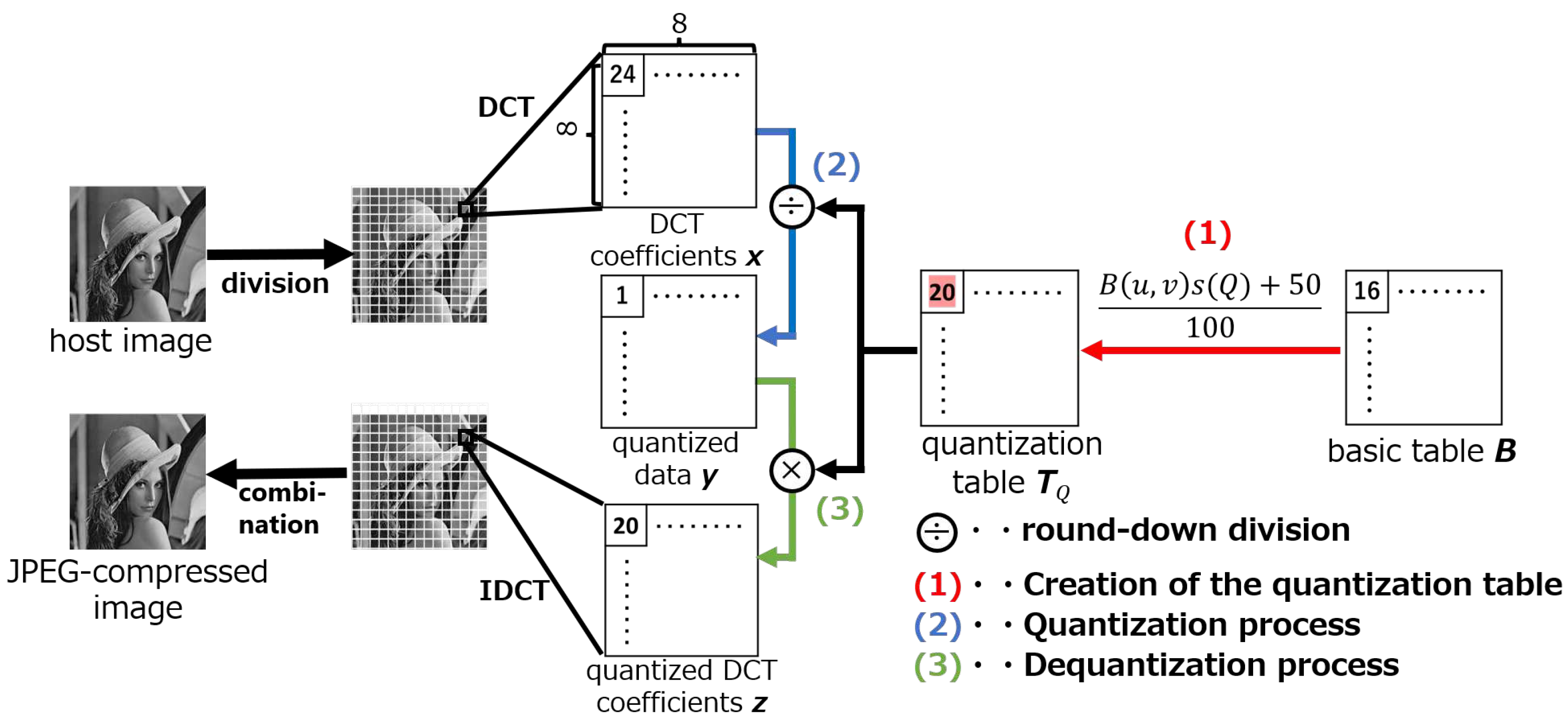
Figure 2.
Overview of the quantized activation function: with slope and number of hyperbolic tangent functions, .
Figure 2.
Overview of the quantized activation function: with slope and number of hyperbolic tangent functions, .
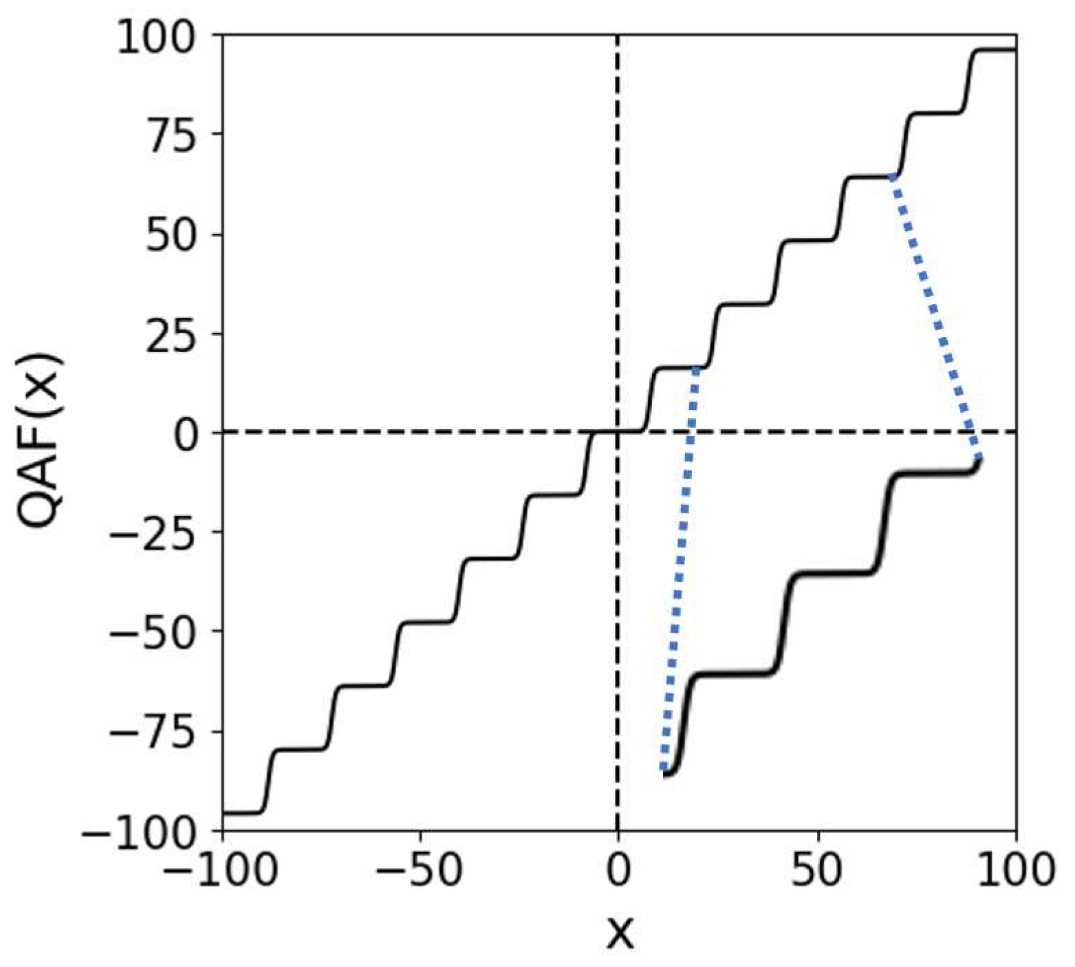
Figure 3.
Overall structure of ReDMark [4]
Figure 3.
Overall structure of ReDMark [4]
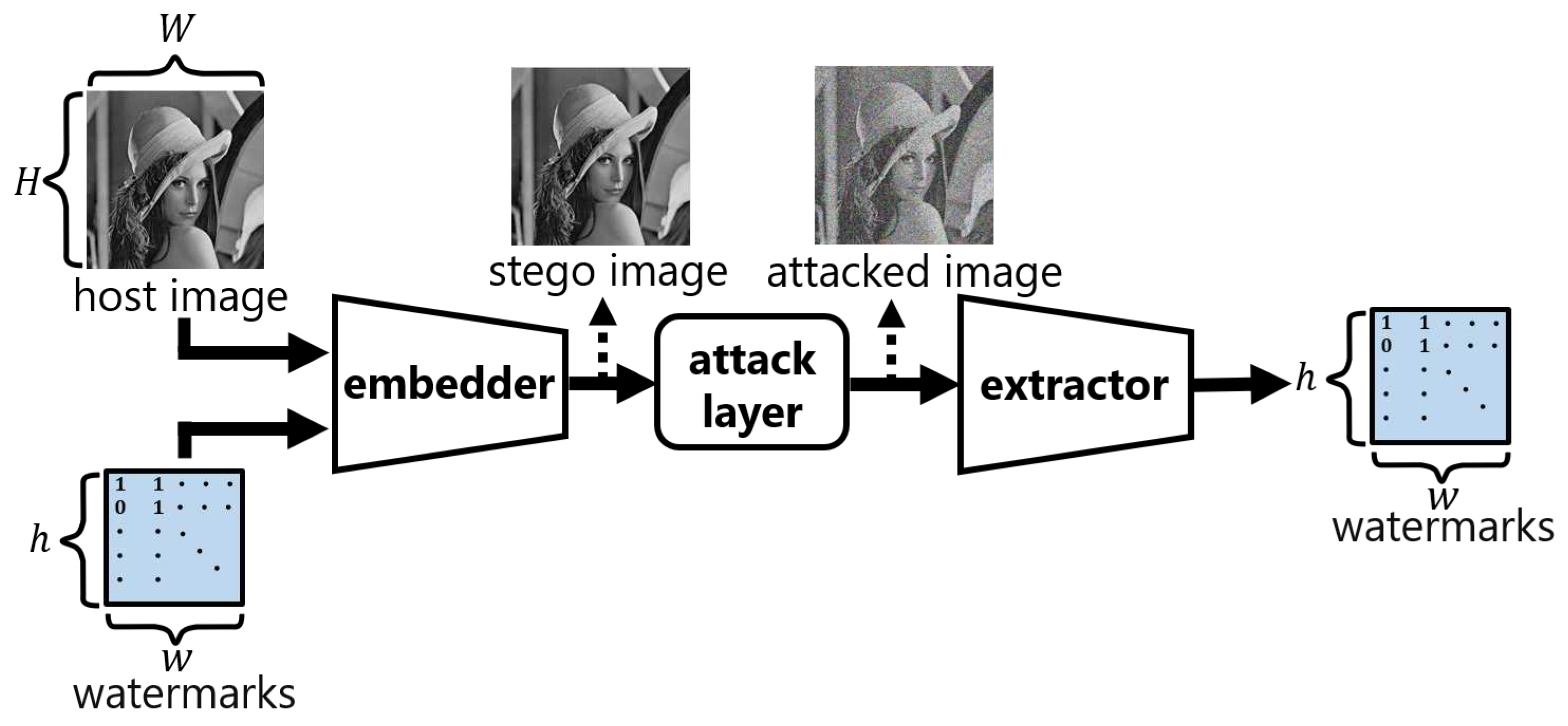
Figure 4.
Embedding network of ReDMark [4]
Figure 4.
Embedding network of ReDMark [4]
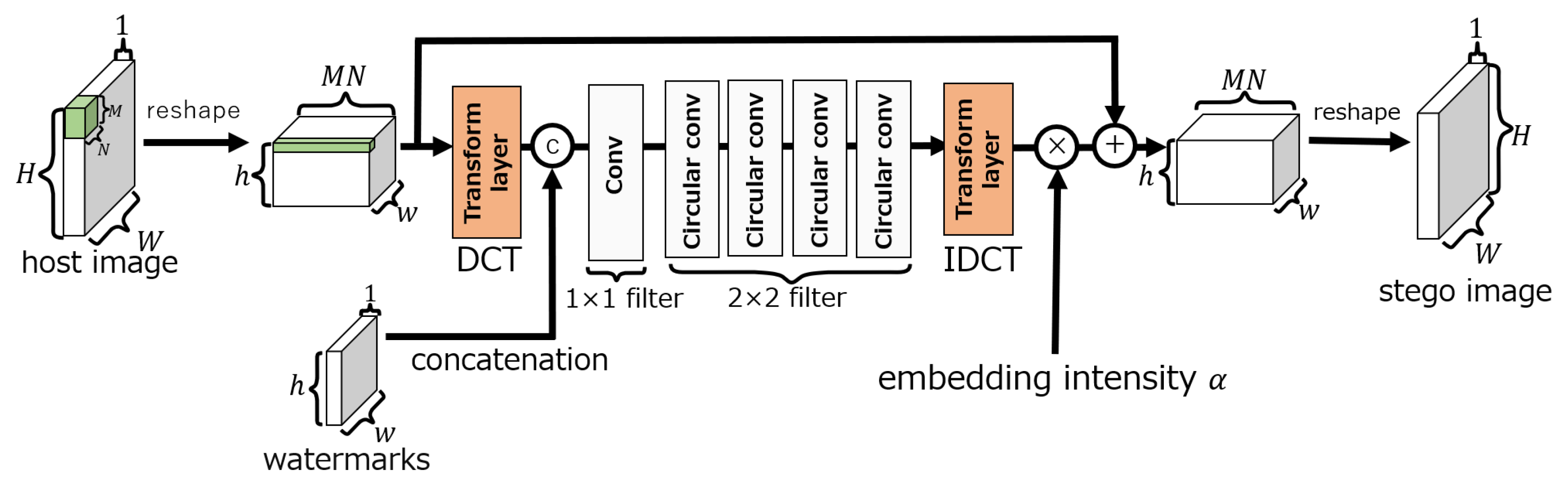
Figure 5.
Extended input in a circular convolution layer. ➀ Extended in the column direction. ➁ Extended in the row direction.
Figure 5.
Extended input in a circular convolution layer. ➀ Extended in the column direction. ➁ Extended in the row direction.
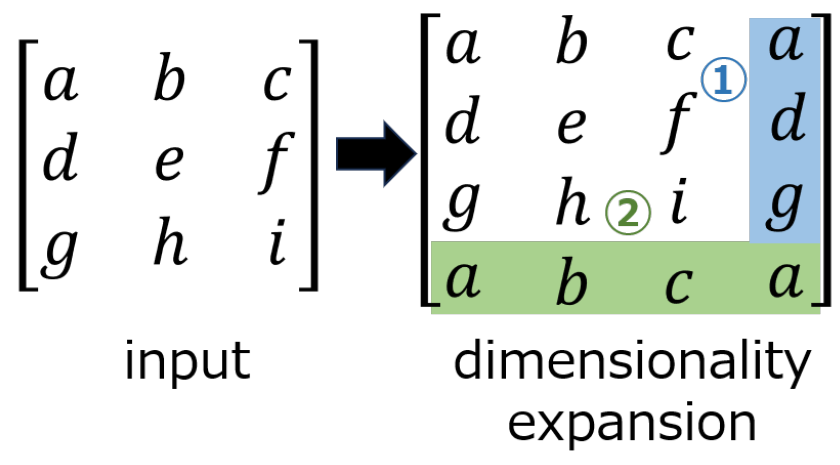
Figure 6.
Extraction network of ReDMark [4]
Figure 6.
Extraction network of ReDMark [4]
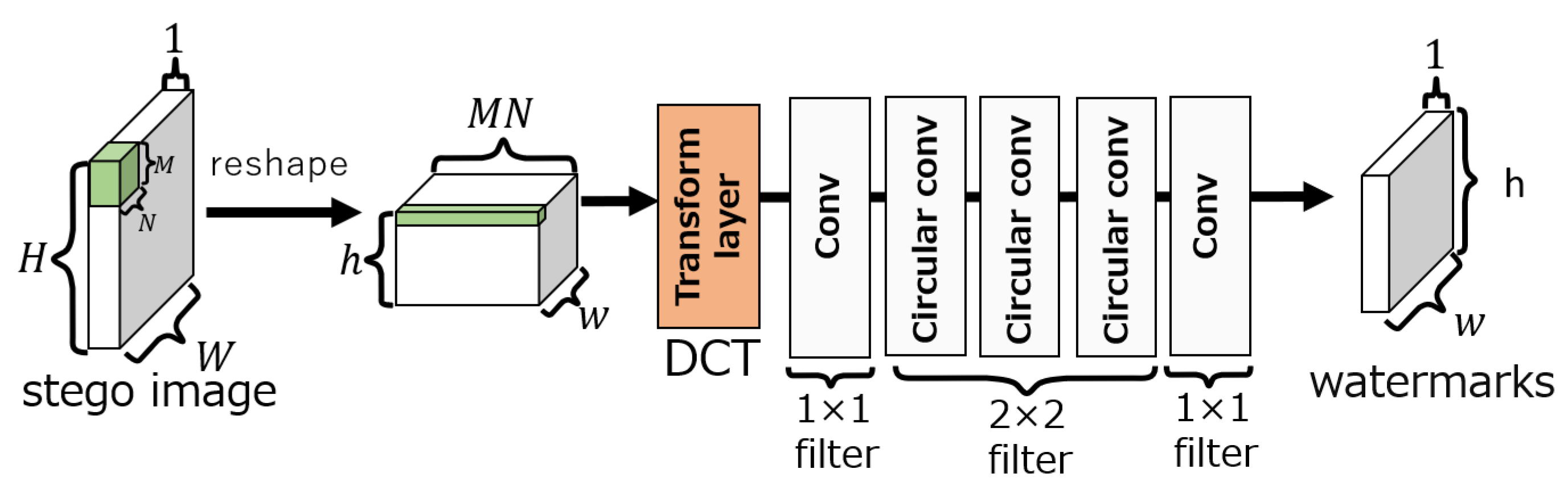
Figure 7.
Proposed attack layer
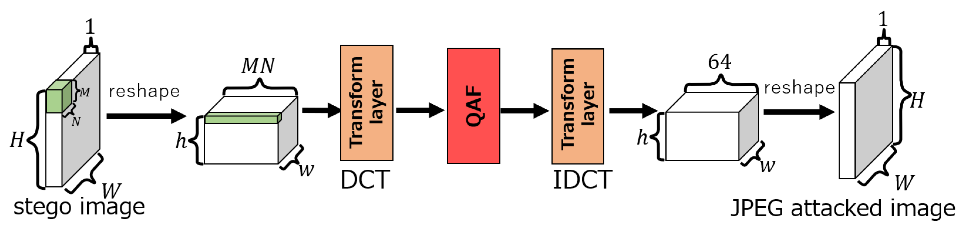
Figure 8.
Original images
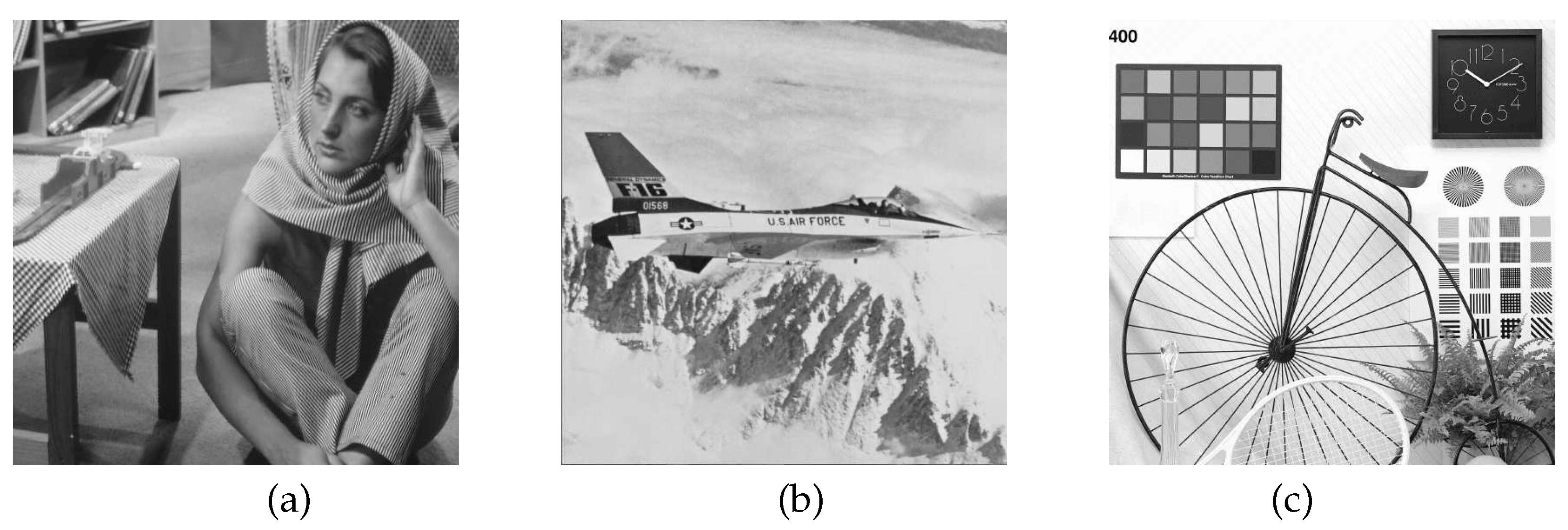
Figure 9.
QAF-applied images and PSNRs
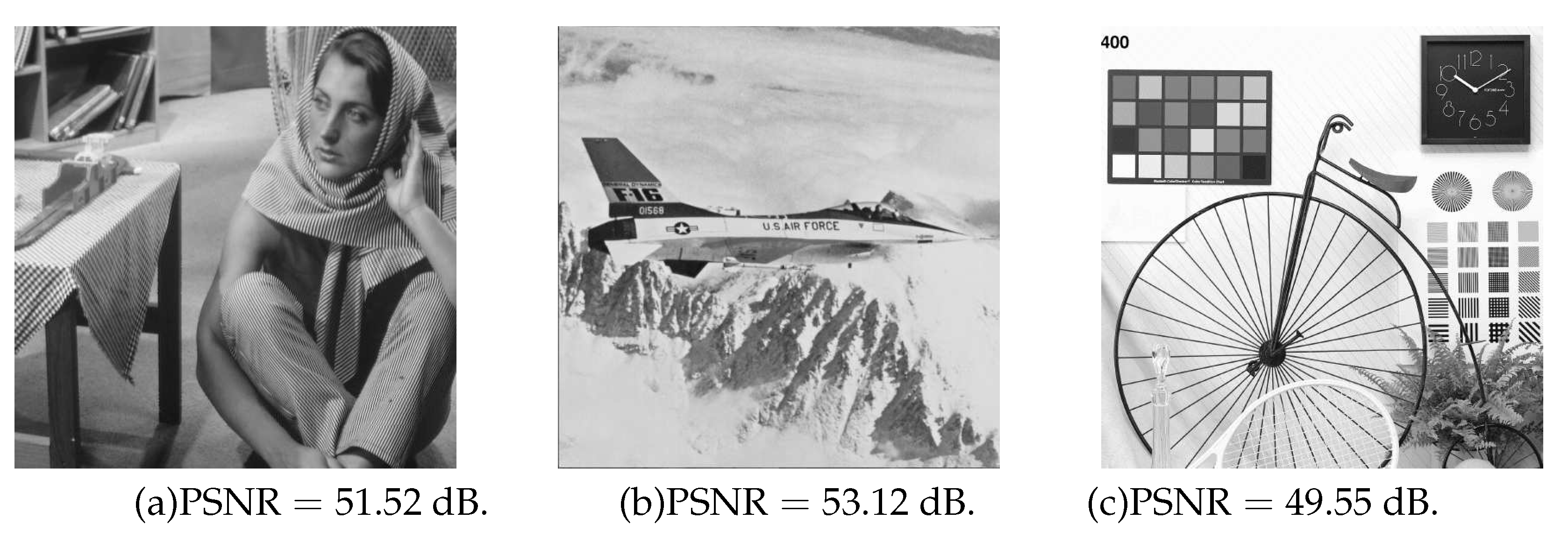
Figure 10.
Image quality of stego-images
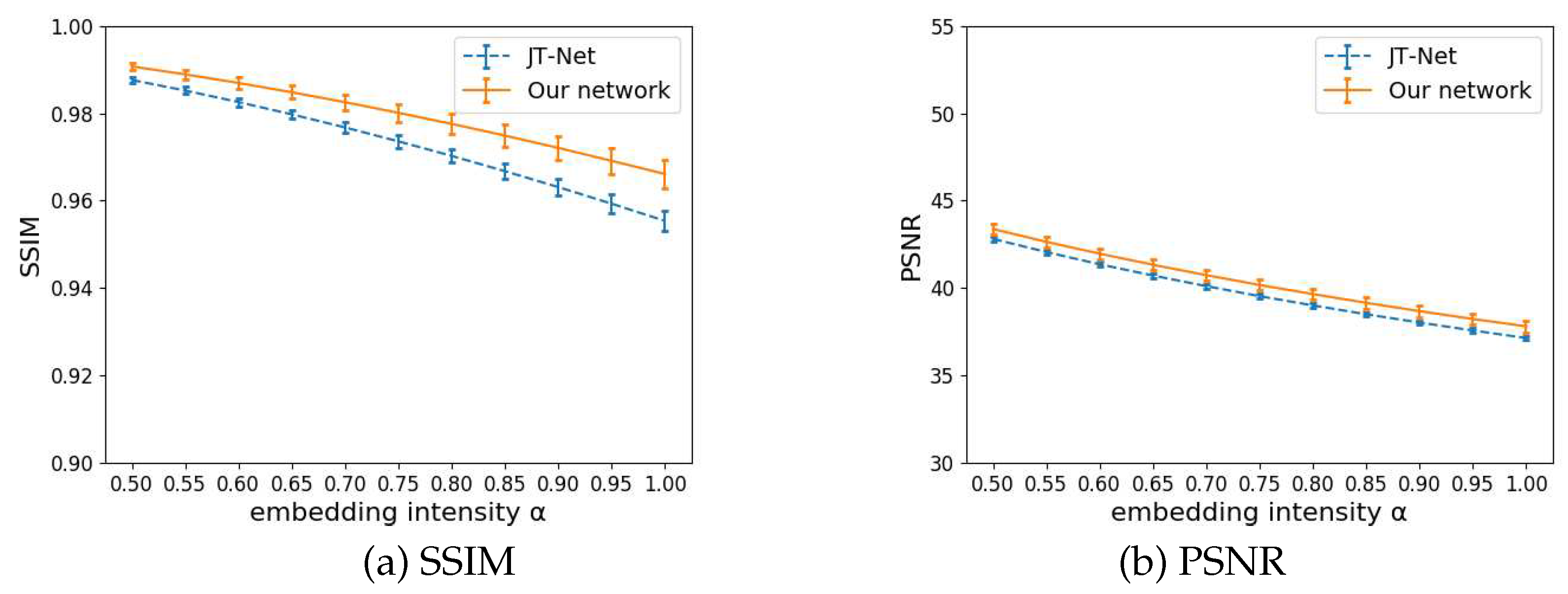
Figure 11.
BER for embedding intensity
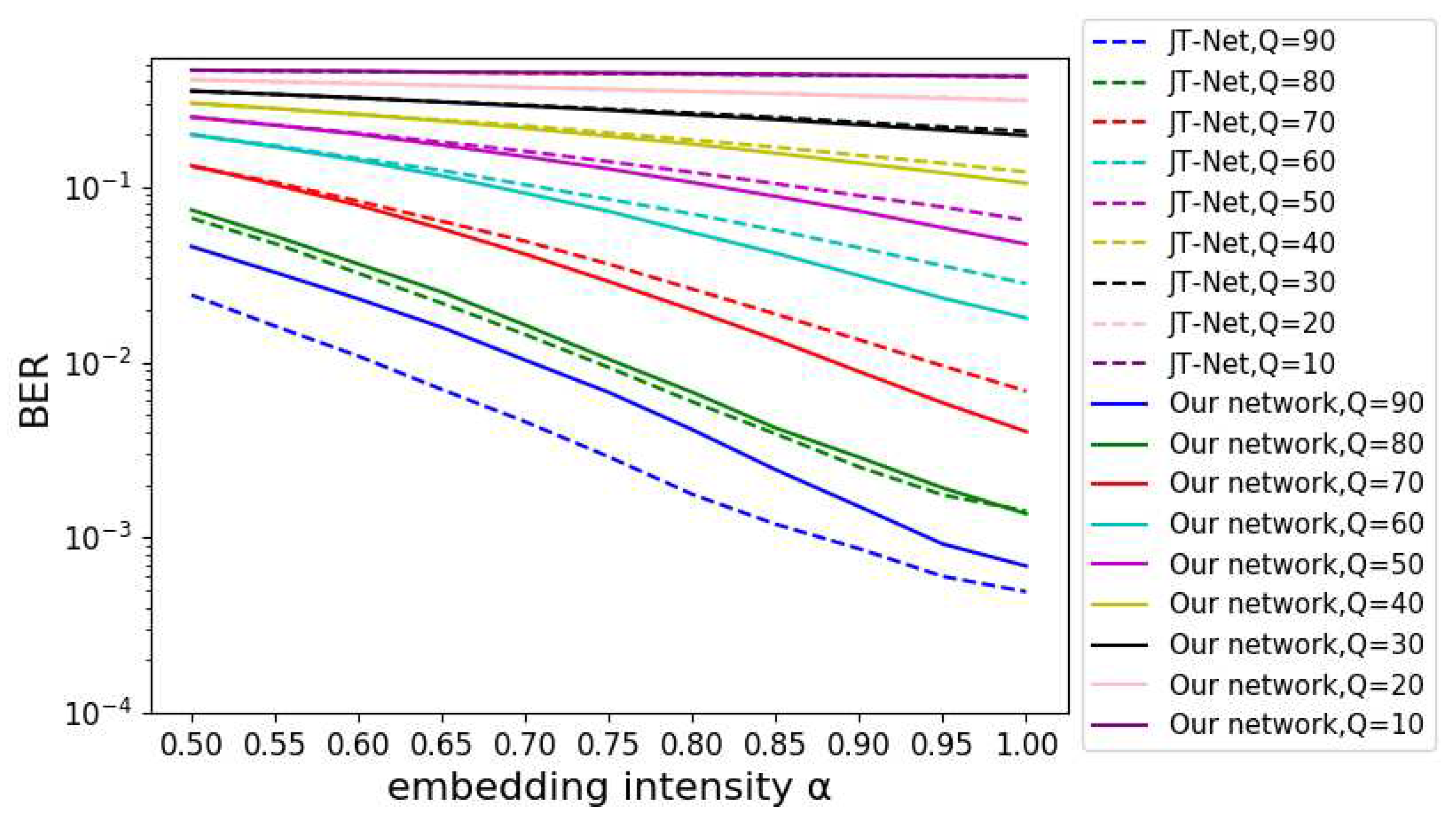
Figure 12.
BER for the JPEG compression lebel Q
Disclaimer/Publisher’s Note: The statements, opinions and data contained in all publications are solely those of the individual author(s) and contributor(s) and not of MDPI and/or the editor(s). MDPI and/or the editor(s) disclaim responsibility for any injury to people or property resulting from any ideas, methods, instructions or products referred to in the content. |
© 2024 by the authors. Licensee MDPI, Basel, Switzerland. This article is an open access article distributed under the terms and conditions of the Creative Commons Attribution (CC BY) license (http://creativecommons.org/licenses/by/4.0/).
Copyright: This open access article is published under a Creative Commons CC BY 4.0 license, which permit the free download, distribution, and reuse, provided that the author and preprint are cited in any reuse.


