
Submitted:
06 February 2024
Posted:
07 February 2024
You are already at the latest version
Abstract
Autonomous driving navigation relies on diverse approaches, each with advantages and limitations depending on various factors. For HD maps, modular systems excel, while end-to-end methods dominate mapless scenarios. However, few leverage the strengths of both. This paper innovates by proposing a hybrid architecture that seamlessly integrates modular perception and control modules with data-driven path planning. This innovative design leverages the strengths of both approaches, enabling a clear understanding and debugging of individual components while simultaneously harnessing the learning power of end-to-end approaches. Our proposed architecture achieved 1st and 2nd place in the 2023 CARLA Autonomous Driving Challenge’s SENSORS and MAP tracks, respectively. These results demonstrate the architecture’s effectiveness in both map-based and mapless navigation.
Keywords:
Autonomous driving
; hybrid architecture
; modular architecture
; end-to-end
; path planning
; CARLA simulator
; Intelligent and Autonomous Vehicles
1. INTRODUCTION
There are different methodologies for developing an autonomous system, which involves software components and algorithms from fields such as machine learning, computer vision, decision theory, probability theory, and more. This mix of components adds complexity to both the development and evaluation process [1]. Figure 1 illustrates the main difference between the three approaches for architecture, being modular, end-to-end, and hybrid architectures.
The standard method employs modular pipelines and has proven effective in scenarios with access to detailed high-definition (HD) maps or dense waypoints. This approach, widely adopted by both companies and research groups [2], decomposes the navigation problem into specific tasks such as localization, object detection, tracking, prediction, decision-making, path planning, and control [3,4,5]. The advantage of this architecture lies in its interpretability, enabling a comprehensive evaluation of each component. However, the extensive coupling of numerous components increases the risk of error propagation, leading to increased complexity in maintaining the entire architecture and a rise in associated costs.
Conversely, the end-to-end approach aims to directly map sensor input to driving actions, bypassing explicit task decomposition [6]. This model leverages deep learning techniques, employing neural networks to learn complex mappings from raw sensor data to steering, brake, and throttle commands. While this method simplifies the system architecture and reduces the need for manual feature engineering, it often requires vast amounts of training data and lacks transparency in decision-making processes. Therefore, by combining modular and end-to-end methodologies, the hybrid approach aims to achieve a balance between the interpretable nature of modular systems and the learning capabilities of end-to-end models. This integration offers potential benefits in system robustness, flexibility, adaptability, and performance.
Another challenge in autonomous driving is evaluating the autonomous driving architecture, whether it adopts a modular, end-to-end, or hybrid methodology. Kalra and Paddock [7], Koopman and Wagner [8], and Huang et al. [9] suggest that to comprehensively assess an autonomous system, it is important to combine real-road and simulation tests. In this regard, simulators offer advantages by creating repeatable scenarios for component performance assessments. They simulate diverse driving situations with realistic dynamics, including weather conditions, sensor malfunctions, traffic violations, hazardous events, traffic jams, and crowded streets. Simulations also serve as effective benchmarks, enabling the evaluation of different system approaches under the same conditions for comparative analysis.
This paper introduces an autonomous driving software architecture employing a hybrid methodology, integrating modular perception and control modules with data-driven path planning. The architecture was designed and evaluated during the 2023 CARLA Autonomous Driving Challenge (CADCH)1 2, achieving 1st and 2nd place in the SENSORS and MAP tracks, respectively3. The 2023 CADCH represents the fifth edition of the autonomous driving competition set in urban simulated environments using the CARLA, featuring diverse urban scenarios. Our involvement spans multiple editions, and we secured victory in the inaugural challenge through a modular and vision-based navigation stack [10]. Therefore, the primary contributions of this paper are:
- A hybrid software architecture for autonomous vehicles, combining modular perception and control modules with data-driven path planning;
- A comprehensive comparison between modular and hybrid software architectures through the simulation of urban scenarios;
- Evaluation of autonomous driving performance in diverse and hazardous traffic events within urban environments.
The remainder of the paper is organized as follows: Section 2 provides a critical overview of related-works; Section 3 describes the modular software architecture developed in the competition; Section 4 presents the hybrid architecture approach; Section 5 discusses the results of the competition and other experiments; finally, Section 6 addresses the final remarks and suggests some future work.
2. RELATED WORKS
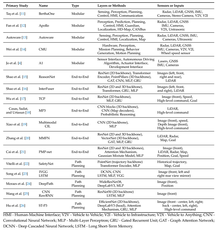
As mentioned before, there are different approaches to developing autonomous systems, depending on the technologies used and how the components are structured. This section offers a brief and critical review of modular, end-to-end, and hybrid software architectures. Table 1 summarizes the related works.

Table 1.
Summary of Related Works.
 |
2.1. Modular Navigation Architecture
A modular architecture typically organizes software components in a hierarchical manner based on specific criteria. Each group, referred to as a layer, operates at a distinct level of abstraction and provides services to its adjacent layers. This structure follows a descending order of abstraction, where higher-level layers handle more abstract tasks, while lower-level layers manage finer controls in the architecture. For example, following the hierarchical navigation stack proposed by Paden et al. [27], the initial layer is responsible for road and lane-level route planning, determining the roads and lanes the vehicle must follow to reach its destination. Subsequently, a behavior layer makes tactical decisions for the vehicle during navigation, such as interactions with other traffic participants, adherence to traffic rules, and high-level maneuver choices (e.g., lane following, lane change, U-turn, overtaking, and emergency stop). In addition to the route, this layer also receives perception information, including obstacle position and velocity, and traffic light status. Once the behavior is determined, a motion planning layer calculates short-term, feasible, and collision-free trajectories, that are translated into low-level commands, such as throttle, brake, and steering, by low-level controllers within the control layer [28].
This design pattern is widely utilized in autonomous systems and has demonstrated notable success in both industrial and research vehicle applications [2]. Key studies typically adopt similar layers, including sensing, perception, planning, control, and human-machine interface as fundamental components [4,11,12,13,14]. However, there are variations, such as communication between vehicles (e.g., Vehicle-to-Anything - V2X) [11], Health Management Systems focusing on hardware and software component monitoring, diagnosis, prognosis, and fault recovery [4,12,14], behavior or mission planning [4,13,14], and mapping strategy [4,11,13]. In the latter case, Wei et al. proposed an alternative to the hierarchical navigation stack. This alternative organizes components of the behavior and control layers in parallel order, based on the functioning of ADAS (Advanced Driver Assistance) system. According to the authors, this approach enhances the flexibility of the autonomous system, enabling it to operate at a higher frequency compared to alternative methods.
Nevertheless, the parallel design faces challenges in coordinating components during complex tasks and maneuvers due to asynchronous communication. Additionally, both parallel and hierarchical approaches share issues related to error propagation between components and the intricate management of components with the increase in vehicle autonomy. This occurs because, as autonomy increases, the vehicle also performs more tasks (e.g., maneuvers) and encounters a broader range of traffic scenarios. Therefore, the number of components adversely affects the system’s performance.
2.2. End-to-End Autonomous Driving
End-to-End is a navigation approach where neural networks and deep learning models are trained to map sensory input (e.g., images or point clouds) to control outputs (e.g., steering, throttle, brake) or intermediate outputs (e.g., trajectory segment). This eliminates the need for manual feature tuning in modular navigation pipelines. The advantage lies in leveraging deep learning generalization to simplify and enhance the adaptability of navigation stacks across different traffic scenarios. There are various approaches to classifying end-to-end models, ranging from the degree of the deep learning model’s involvement in tasks to the technology applied. In the former category, methods range from pure end-to-end architectures, where the deep learning models handle the entire mapping and decision-making process, to hybrid approaches that integrate different algorithms, such as probabilistic models, control theory, fuzzy inference systems, etc. The latter category divides models based on techniques, such as imitation learning and reinforcement learning.
In addition to the presented taxonomy, studies on end-to-end navigation also focus on input representation aspects and the model design. This includes considerations in the number of cameras (e.g., single or multi-camera setups) [15,16,17], methods for 3D data representation (e.g., point cloud or Bird’s Eye View images) [15,16,18,20], sensor fusion and multimodality (e.g., different sensors and feature fusion methods) [19,20,21], interaction with traffic agents (e.g., interaction graphs or grid maps) [15,20], deep learning technologies (e.g., transformers, graph neural networks, deep reinforcement learning, attention mechanisms, generative models, etc.) [15,16,20,21], decision-making within the network (e.g., high-level commands input or inference) [17,18], and the accuracy or feasibility of the output (e.g., using standard controllers to estimate final outputs or filtering the output of the deep learning model) [15,18,21].
In summary, end-to-end models primarily rely on RGB images and LiDAR-generated point clouds, represented in 3D as points, voxels, or Bird’s Eye View (BEV) images. While the ResNet network is commonly used for feature extraction from images and BEV [16,17,18,20,21], some studies also explore the use of specialized deep learning models for 3D data, such as PointPillars [15] and VectorNet [20]. Two significant challenges for deep learning models include multimodality fusion and how to handle tactical decisions within the network (or when incorporating decisions from external sources). In the former case, early-fusion and middle-fusion approaches are noteworthy [19], they often involve attention mechanisms or concatenation of feature vectors. In the latter case, tactical decisions (i.e., high-level commands) can be treated as an input modality [17] or a conditional variable [18,19], particularly in approaches exploring multiple-expert designs. However, both pure and hybrid end-to-end navigation methods still face challenges related to the lack of transparency and explainability in decision-making and the requirement for extensive training data.
2.3. Data-driven Path Planning
Autonomous vehicles rely on path planning algorithms to navigate through dynamic and complex environments. Data-driven approaches have gained prominence in recent years, representing a shift from traditional rule-based methods [29]. In data-driven path planning, algorithms leverage machine learning techniques to learn collision-free paths from large datasets [30]. These datasets typically include information from various sensors, historical driving experiences, and diverse environmental conditions. Similar to end-to-end navigation architectures, data-driven path planning also inherits the adaptability features from deep learning models, which make them able to plan under diverse road geometry and traffic scenarios.
Techniques for data-driven path planning typically emphasize the representation of spatial and temporal features. However, to address the challenges of dynamic driving scenarios, they also consider the representation of traffic rules, interaction among traffic participants, output trajectory smoothness and comfort, high-level commands (e.g., maneuvers), and variations in road geometry. Spatial features are commonly derived from frontal camera images or Bird’s Eye View (BEV) projections, using CNN-based networks for feature embedding [23,24,25,26]. Some works also use the historical trajectory of the ego-vehicle and surrounding agents [22]. Temporal features are traditionally addressed by recurrent neural networks (e.g., GRU and LSTM) [23,25,26], although recent studies have explored the application of Transformer networks [22]. Semantic and abstract data, such as traffic rules and high-level commands, are integrated as feature vectors or conditional variables [26]. Finally, ensuring trajectory smoothness typically involves the application of a post-processing algorithm or the penalization term in the loss function [26]. Nevertheless, methods employing machine learning for path planning face challenges in terms of transparency and explainability. Moreover, there is room for improvement in addressing global planning, high-level commands, managing dangerous and unexpected driving scenarios, and ensuring dynamic and kinematic feasibility of planned trajectories.
In this context, this paper introduces a hybrid autonomous vehicle architecture that integrates modular pipelines with data-driven path planning, offering a comprehensive comparison of these approaches. This architecture, developed and evaluated in the 2023 CARLA Autonomous Driving Challenge (2023 - CADCH), secured 1st and 2nd place in the SENSORS and MAP tracks, respectively. By combining modular perception and control components, it delivers reliable information to the data-driven path planning, ensuring the generation of kinematically feasible trajectories. Additionally, an early-fusion approach enhances the spatial and semantic representation of the environment in the data-driven path planning through the fusion of LiDAR Bird’s Eye View images, Stereo Camera projections, and high-level commands. The results demonstrate the network’s generalization capabilities with real-time inference, highlighting the architecture’s reliability.
3. PROPOSED MODULAR PIPELINE
An autonomous system requires several components and its architectural design provides an abstract view of the system operation and organization. In a layered architecture, the components have public and well-defined communication interfaces through which they exchange information with other components. This characteristic enables the definition of a common architecture for all tracks in this challenge, through adjustments of few components for the maintenance of the same communication interface. This strategy reduces the time spent on the development of the agents, and enables the evaluation of the autonomous navigation performance with different sensors and algorithms for a specific task.
Figure 2 shows the general software architecture designed for all agents of LRM team in the 2023 CARLA Autonomous Driving Challenge. The name "CaRINA Agent" is used to refer to this architecture in the rest of this paper. The layers of the architecture are sensing, perception, map, risk assessment, navigation, control, and vehicle. Robotic framework ROS (Robotic Operating System)4 supported the communication interface between components with Publish/Subscribe pattern for messages passing [31].
3.1. Mapping and Path Planning
A map is an essential component enabling the autonomous vehicle to execute its tasks safely and efficiently, storing diverse information, beneficial for various components of the autonomous system [32]. This includes the road geometry description for path planning and the topological representation of roads and intersections, commonly referred to as the road network, used for route planning. In addition to static object positions, navigable areas, positions of traffic signs and lights, traffic rules, and semantic information related to the road. In this architecture, we employed the OpenDRIVE [33,34] map standard to assist the navigation and perception components.
3.1.1. OpenDRIVE
The OpenDRIVE is an open format to describe road networks, using XML version 1.0, which is able to represent the road geometry as well as the context information of roads that may influence the behavior of vehicles driving in it, such as traffic signs, traffic lights, and the type of roads and lanes (e.g. highway and sidewalk) [34,35]. The format description is built on a hierarchical structure with four main elements: header; road; junction; and, controller. Figure 3 shows the visualization of the OpenDRIVE map after being parsed by the map manager in the architecture.
The header, is the first element of the description and holds metadata of the map, such as the name or a geographic reference for transformations between the Cartesian and Geodesic coordinate systems. The road element encompasses geometry description and additional properties (e.g., elevation profile, lanes, and traffic signs). The properties such as traffic signs are placed with respect to the distance to the initial point of the lane, using a local coordinate system. Besides that, roads can connect directly or through intersections using the junction component, preventing ambiguities in connections. Lastly, a controller is employed for signalized junctions or other road elements imposing control on the vehicle.
3.1.2. Path Planning
Path planning is responsible for determining a feasible and optimal path from a starting point to a destination in a given environment. This planned path considers factors such as road geometry, static and dynamic obstacles, vehicle physical constraints, and criteria like time, speed, fuel efficiency, or safety. Various algorithms, including rule-based, gradient-based, graph-based, and optimization methods, can perform these tasks. In addition, recent studies have explored the integration of machine learning into path planning. Moreover, the task can be divided into two steps: global planning and local planning. Global planning estimates a reference path, considering static features (e.g., road geometry and static obstacles) and the intended route. Local planning adjusts this global reference path based on dynamic variables in the traffic scene, such as dynamic obstacles.
In the modular navigation pipeline strategy, global reference planning incorporates a local speed profile based on the dynamic scene, along with local lane-change planning due to traffic events. The global reference planning involves sparse waypoints representing the intended route. Subsequently, lane-level localization determines the corresponding lane and road ID for each waypoint using the OpenDRIVE map manager. This information enables the system to estimate a lane-level route, identifying the roads and lanes the vehicle must traverse to reach its destination. Finally, segments of the reference path, each spanning 50 meters, are published in the ROS ecosystem based on the vehicle’s speed and current position.
3.2. Perception
The autonomous driving systems proposed in this paper relies on two types of sensors for robust environmental perception: a stereo camera and a LiDAR sensor. Our proposed perception system, depicted in Figure 4, adopts a multi-sensor fusion approach to achieve accurate and robust object detection in 2D/3D images and point clouds. This approach employs distinct detection modules and their fusion, each capitalizing on the strengths of different sensor modalities:
•Height map: As a basic obstacle detector, we employ a height map generated from the LiDAR point cloud, similar to the one presented in [36]. This method analyzes height differences in a grid, identifying obstacles exceeding a threshold. Grid cells with no such differences are deemed part of a plane. We use a polar grid map and a 20 cm as threshold. This detection mechanism serves as a backup for emergency situations. The first branch in Figure 4 depicts a height map-based perception process, where points are assigned colors based on their height to create a visual representation of the surrounding environment’s topography then grid cells within that contain points exceeding the predetermined vertical distance threshold are identified. Finally, points situated within these designated grid cells are marked in red to clearly indicate potential obstacles. Our obstacle detector using height map in a polar grid is open source and available online5.
•Instance segmentation: For object detection, we employ Mask R-CNN [37], a powerful instance segmentation algorithm that extracts coordinates of bounding boxes and masks for each object instance detected in the image. Our system categorizes these objects into eight categories: car (including vans, trucks, and buses), bicycle (including motorcycles), pedestrian, red traffic light, yellow traffic light, green traffic light, stop, and emergency vehicle. Code is open source and available online6.
•Fusion with stereo camera: Since the image used for instance segmentation is also the left image of the stereo camera, we leverage this for 3D detection and classification. The bounding box coordinates and pixel mask of each object instance detected in 2D are mapped to corresponding 3D points in the organized point cloud. This 3D point cloud inherits the color and the image’s row, column structure but expands it with 3D/depth information. This fusion process creates an RGBD point cloud with color and 3D/depth information for each object instance, enabling accurate classification and positioning.
The third branch, Figure 4, illustrates an example of a point cloud constructed from the stereo camera, while the fourth branch shows an example of instance segmentation corresponding to the same scenario. Finally, the fusion of these two branches enables the detected objects to be mapped onto the RGBD point cloud, providing a comprehensive visualization of their positions within the 3D environment.
While this method can detect both static and dynamic objects, it is not the primary system detector in our architecture due to its non-real-time operation with a maximum of 5 frames per second. Nevertheless, the detailed information it provides on traffic light states, unavailable from LiDAR, justifies its inclusion despite the latency. Dynamic object detection (cars, bicycles and pedestrians) in this fusion serves as a backup for emergencies, and we currently do not track these objects.
•3D detection in point clouds (dynamic objects): For 3D detection in LiDAR point clouds, we leverage the PointPillars algorithm [38]. This algorithm provides regression of 3D bounding boxes of objects and their orientation related to the ego vehicle. PointPillars demonstrates commendable performance in real-world autonomous driving scenarios. Its pillar representation retains valuable spatial information while maintaining computational efficiency, a critical factor for real-time applications. Moreover, it effectively leverages the strengths of LiDAR data, including its ability in handling occlusions and performing reliably in diverse lighting conditions.
•Tracking: The perception stack (in point clouds) detailed in this section, which supplies inputs to the risk assessment module responsible for determining FSM graph states, consists of two integral components: (i) pose estimation (bounding boxes) and (ii) multi-object tracking (MOT) modules. Having a stable and precise state estimation, both for the ego-vehicle and dynamic objects in the surroundings, is important to transition across the states.
Regarding the multi-object tracking module, we based on the one proposed by [39]. This approach, known as Simple Online and Realtime Tracking (SORT), divides the tracking task into three sub-tasks: detection, data association, and state estimation.
As detailed earlier, objects are detected in the LiDAR frame using PointPillars. This detection model differs from the ones adopted originally by the SORT tracker. The detected objects’ bounding boxes are projected into the world frame using the ego-vehicle estimated pose, and their respective poses are matched in the data association step. At this point, we keep the SORT tracker data association in the 2D space, in which we compute the intersection over union (IoU) of the top-down projection of the bounding boxes. Our assumption is that two dynamic objects do not overlap in the X-Y plane.
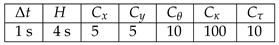
As for the state estimation, we use a Kalman Filter-based approach, in which our goal is to estimate the 3D position of the bounding box center , 3D dimensions of the bounding box , the yaw angle , and the 3D velocities of the tracked object in the International System of Units and in the global reference frame. This space state differs from the SORT paper state, in which the estimated state is performed in the pixel space. Also, notice that the vehicle pose estimation is important in this step, as we are tracking in the global reference frame.
As we represent this state vector as , we need to define both the state propagation and observation model matrices.
The state propagation we adopted assumes constant linear velocity between detections so that we can propagate the position using the propagation matrix F from Equation 1.
where I represents the identity matrix, 0 the zero-filled matrix, and represents the period between predictions. The subscripts indicated with represent the matrix number of rows M and columns N, respectively.
Regarding the observation model matrix, since we obtain directly the 3D position, dimensions, and yaw angle from our detection module, our observation matrix is defined by .
The third branch in Figure 4 illustrates detection and tracking in 3D, with LiDAR serving as input to the 3D detector. In our case, the 3D detections of point pillars are fed into the SORT algorithm, which we have modified for tracking. Ultimately, for visualization, each tracked object is assigned a distinct color.
•Prediction: Our system employs a prediction-based approach to ensure safe navigation by anticipating the movements of surrounding objects. This approach utilizes a simple motion model based on the object’s current speed, as estimated by the tracking system and this model assumes constant velocity for each object, providing a first-order approximation of their trajectories.
The prediction formula for a linear motion model is defined by the Equation 2.
Where is the current pose, v the actual velicity of the surrounding object and represents the time interval for prediction (5 seconds). Finally is the predicted pose in the interval .
While more complex prediction models exist, opting for a simple linear model ensures computational efficiency. This linear motion model for future pose prediction demands fewer computational resources, making them suitable for real-time applications in autonomous driving.
3.3. Risk assessment
Our autonomous driving system employs a dedicated Collision Risk Assessment (CRA) module to continuously evaluate potential threats posed by both dynamic (cars, pedestrians, bicycles) and static surrounding objects. This module integrates current and future positions of surrounding objects, obtained from the previous stage, with the ego vehicle’s planned path for risk assessment.
•Zoned Risk Evaluation: The planned path is divided into two zones, each reflecting different risk levels based on distance from the ego vehicle: a High Risk Zone (0-4m) and a Moderate Risk Zone (4m-40m). For risk evaluation: The path ahead is divided into two zones, each carrying different risk levels based on Euclidean distance. These zones are corridors created from the waypoints of the planned path (essentially buffer zones extending 40 meters ahead of the ego vehicle). The width of these corridors matches the width of the ego car.
Any object (static or dynamic) whose current position intersects either zone is considered a potential collision threat. The intersection point of predicted trajectories with the ego vehicle’s path is also considered. We assume that our lateral MPC controller guarantees that the ego car will pass exactly through these corridors.
The identified potential points of collision and object’s information, including type, distance, and predicted trajectory, is reported to the decision-making module for determining appropriate speed adaptations. Figure 5 visually illustrates the risk assessment process, showcasing three points as examples. Note that other surrounding objects and their predicted trajectories are currently ignored unless they enter the relevant risk zones or directly influence the planned path.
3.4. Decision making
The decision-making module utilizes a synchronous Moore Finite State Machine (FSM) to orchestrate actions based on inputs from the Collision Risk Assessment (CRA) module. The FSM employs a binary encoding scheme for inputs as shown in Table 2
The FSM comprises four key states, each governing specific speed control behaviors:
•Drive State (S1): No obstacles impede the vehicle’s progress. Target speed is set to a maximum of 8.8 m/s (31.68 km/h).
•Follow the Leader State (S2): The CRA reports an obstacle (static or dynamic) ahead of the ego vehicle, triggering dynamic speed adjustments. Speed is adjusted based on distance and time to collision (TTC), calculated using the ego vehicle’s current speed and distance to the obstacle.
•Red Light State (S3) and Stop Sign State (S4): These states mirror the "Follow the Leader" logic, utilizing TTC to achieve controlled stops at designated locations. The vehicle decelerates smoothly, ensuring compliance with traffic rules and safety.
Figure 6 depicts the state transition diagram, visually representing the FSM’s logic. The decision-making module employs a straightforward yet effective FSM structure for robust decision-making. Speed control strategies adapt dynamically to varying conditions, ensuring safe and efficient navigation. The module seamlessly integrates with other components of the autonomous driving system, including perception and control modules. The FSM operates synchronously at 10 Hz, aligning with sensory data capture rates.
The current approach uses the actual velocity of the ego vehicle to calculate TTC, after which velocity adjustments are made to prevent collisions. This method is simple, fast, suitable for quick estimations, easy to implement, and computationally efficient. -However, it assumes constant velocity and ignores potential future trajectory changes. The TTC formula is:
3.5. Control
The control layer generates steering, throttle, and brake commands to keep the agent on the planned trajectory. This goal is achieved through two closed-loop control mechanisms that receive desired vehicle trajectory information from the navigation layer’s decision-making and local path planning modules. These modules set desired trajectory and velocity into the agent’s action space. The closed-loop controls translate reference values into actual control actions for braking, throttle, and steering, which are then sent directly to the simulator for execution.
For longitudinal control, the decision-making module (FSM) calculates the desired agent’s velocity, which is used to compute the final velocity. A Proportional-Integral-Derivative (PID) controller then ensures the agent follows this desired reference.
3.5.1. Lateral Control (MPC)
Lateral control, responsible for generating the steering signal, leverages Model-Based Predictive Control (MPC). This approach optimizes a cost function across a predefined time horizon, H, resulting in a sequence of actions, one for each time step (). The immediate action is executed, and the process restarts in the next time step, employing a receding horizon optimization strategy.
The constraints that delineate the vehicle’s motion model are fundamentally non-holonomic. Car-like robots have the flexibility to occupy positions on the 2-D plane, adopt various headings, and utilize different steering angles, resulting in up to four degrees of freedom. Nevertheless, these constraints impose the following two kinematic limitations: a) the vehicle is restricted to movement solely in the forward and backward directions, and b) the steering angle is subject to bounds [28]. Consequently, the actual motion of the car and the trajectory planned may differ when the planner neglects dynamic factors.
Table 4.
Non-linear MPC parameters.
 |
By considering that the wheels roll without slipping, only the kinematic equations can be considered and the lateral dynamic effects can be neglected [40]. Therefore, the considerations made so far result in the following kinematic model [41]
where . The motion constraints are added to the optimization problem by means of the third power of on the basis of Eq. 3 [42], where v is computed by the decision-making module (considered constant in the optimization). The cost function is defined as the sum of the quadratic differences between the decision variables and the reference path,
and also, the quadratic of
where , , , and are cost weights manually tuned.
3.6. Localization
In order to perform the ego-vehicle pose estimation, we fused the relative transforms obtained using an odometry source (in our case, visual-inertial odometry - VIO), the IMU orientation, and the GNSS position using an Extended Kalman Filter (EKF) approach, as in the Figure 7. The inputs of our stack are the camera image, the IMU orientation, the GNSS coordinates, and the sensor calibration (external reference frames’ relative transformation). The output elements of the pose estimation stack are estimated pose and its uncertainty. The VIO estimation is responsible for estimating , which represents the pose transformation matrix of the current camera frame w.r.t. the previous, and the estimation uncertainty covariance matrix, .
While the GNSS is responsible for providing the global geographic coordinates, the IMU provides the linear acceleration, angular velocity, and 3D orientation at a higher frequency. We then synchronize both the 3D orientation and global coordinates in order to provide , which represents the transformation matrix of the IMU frame w.r.t. the world frame, and its uncertainty, . In our case, the IMU and the GNSS are represented by the same reference frame, but we left them illustrated in the diagram for the sake of clarity. Also, the geographic coordinates provided are then converted to a plane projection coordinate system.
The input poses, and , and the sensor calibrated, are then provided to the EKF and then converted to a common reference frame internally. The goal is to estimate the 6DoF pose of the agent frame w.r.t. the world frame, , where: are the global coordinates, easting, northing, and altitude, respectively; and represents the four components of the quaternion that represents our agent’s orientation. For each relative pose received, , the EKF performs a system prediction, which implies accumulating drift until a global pose, , is received and the state update is performed.
We emphasize that this pose estimation module is also modular, so that the back end (in this case, the EKF), the methods used for estimating the relative transforms, and the source of the global pose estimation do not need to be the same as the ones we used in this project.
In practice, for estimating the relative pose transformations using VIO, we used the RTabMap ROS implementation7. RTabMap is known for its estimation robustness and its full functionalities are widely used in SLAM applications. As for the EKF implementation, we used the GTSAM implementation8. While GTSAM is known for implementing solutions using factor graphs, it also implements a very convenient interface for representing pose transformations and implements the 3D pose Extended Kalman filter off-the-shelf. Finally, our localization stack is open source and available online9.
4. Hybrid Architecture for Mapless Autonomous Driving
This section introduces our hybrid architecture for mapless autonomous driving, designed to navigate challenging scenarios like the CARLA Leaderboard’s SENSORS track. Building upon our modular pipeline described in previous sections, we leverage robust obstacle detection, risk assessment, and decision-making modules while replacing traditional map-based planning with a end-to-end path planner named CNN-Planner [10].
Conventional map-based approaches often struggle in dynamic environments lacking accurate maps. We overcome this limitation by using a improved version of the CNN-Planner for mapless situations. This planner generates a set of waypoints and utilizes sensor fusion in the BEV space as its primary input.
This fusion is named BEVSFusion which is a rich data structure that seamlessly fuses High-level commands and Point clouds.The BEVSFusion structure receives data from three sources that are processed in the following way:
- Stereo Camera: We utilize a pair of cameras with specific field of view, resolution, and baseline. Disparity maps calculated with the ELAS algorithm and projected into point cloud. Stereo point cloud is transformed from the camera coordinate system to BEV coordinate system using the transformation matrix .
- LiDAR: The LiDAR point cloud is directly transformed to the BEV coordinate system using transformation matrix. LiDAR points are then rasterized in an RGB image where a colormap encodes height information (blue for ground, yellow for above sensor). Empty pixels are filled with black.
- High-Level Commands: Global plan commands are converted from the world frame to the BEV frame using and rasterized as colored dots in BEV space (blue for turn right, red for turn left, withe for straight and green for lane follow ). Additionally, we rasterize a straight line connecting two adjacent high-level commands. This connection enhances the representation of the order and sequence of points within the raster, facilitating interpretation and providing additional information to the CNN network.
Finally, these three processed elements (rasterized LiDAR, stereo, and high-level commands) are stacked into a single 9-channel image (BEVSFusion). This unified structure integrates spatial, depth, height, color, and high-level command information for robust path planning.
BEVSFusion serves as the input to CNN of the path planner. The CNN-Planner can be represented as a function:
This CNN is a architecture for regression of a sequence w of dense waypoints for the ego vehicle’s trajectory. Each waypoint in the sequence represents a point with coordinates in the ego-car coordinate system. corresponds to the closest point to the ego car, while denotes the furthest point on the planned trajectory. w is transformed from the ego coordinate system to the world coordinate system using transformation matrix.
Compared to the original CNN-planner implementation, which generates an output of 50 w waypoints, our approach yields 200 w waypoints. These waypoints cover a distance of 40 meters, resulting in a longer path. This extended path not only provides a larger area for monitoring potential issues but also ensures more precise guidance for the vehicle.
Figure 8 visually illustrates the process, highlighting the creation of BEVSFusion through sensor fusion and its integration as input for the CNN-Planner and generating the planned trajectory. Finally the path w in the world coordinate system is followed using a MPC controller.
5. Experiments and results
5.1. Experimental setup
Our research adopts the Robot Operating System (ROS) as the unifying framework for both our modular and hybrid driving architectures. ROS’s publisher-subscriber communication paradigm [43] facilitates efficient data exchange between components, enabling a flexible and scalable system design. The ROS master node indexes and coordinates components, while peer-to-peer messaging enables direct communication between nodes [31]. This structure streamlines the development and integration of multi-component systems, particularly in applications like autonomous driving and robotics.
Our autonomous driving agents implements all modules described, for the perception layer we have:
- Two monocular cameras with 71° field of view (FOV) each are combined to form a stereo camera for 3D perception, producing a pair of rectified images with dimensions of pixels. The baseline of our stereo camera is 0.24 m. We utilize the ELAS algorithm [44] to generate 3D point clouds from the stereo images.
-
LiDAR sensor: 64 channels, 45° vertical field of view, 180° horizontal field of view, 50m range. Our system utilizes a simulated LiDAR collecting around one million data points per scan across 64 vertical layers.LiDAR and stereo camera are centered in the x-y plane of the ego car and mounted at 1.8m height.
- GPS and IMU: For localization and ego-motion estimation.
- CANBus: Provides vehicle internal state information such as speed and steering angle.
Our modular architecture additionally utilizes an OpenDrive map pseudo-sensor for route planning and a ObjectFinder pseudo-sensor, used exclusively for dataset creation, provides ground-truth information about dynamic and static objects within the CARLA simulator.
5.2. Metrics
Autonomous vehicles are heterogeneous and complex systems, orchestrating sensing, perception, decision-making, planning, control, and health management. Evaluating the performance of these complex systems requires a holistic approach, going beyond individual evaluation to assess the harmony of the entire system.
Traditionally, unit tests analyze individual components, seeking malfunctions and quantifying their performance with metrics like accuracy, recall, and precision (e.g., for classification algorithms [45,46]). Integration tests take a broader perspective, examining the interplay between two or more components (e.g., obstacle detection and avoidance). Finally, system tests encompass the entire system, evaluating the harmonious collaboration of all its components [47,48]. However, a standardized methodology for comprehensively assessing and comparing the complete performance of autonomous driving systems remains a challenge. The CARLA Leaderboards offer a standardized benchmark for evaluating autonomous driving systems, providing diverse sensor configurations and software architectures.
These leaderboards immerse the autonomous system, or "agent," in simulated urban environments. Each scenario throws diverse challenges, varying in cityscapes, traffic areas (highways, urban roads, residential areas, roundabouts, unmarked intersections), route lengths, traffic density, and weather conditions. Moreover, each route incorporates traffic situations inspired by the NHTSA’s (National Highway Traffic Safety Administration of the United States) pre-crash typology [49], encompassing diverse scenarios like:
- Control loss without prior action.
- Obstacle avoidance for unexpected obstacles.
- Negotiation at roundabouts and unmarked intersections.
- Following the lead vehicle’s sudden braking.
- Crossing intersections with a traffic-light-disobeying vehicle.
- Leaderboard 2 expands this scenarios, adding:
- Lane changes to avoid obstacles blocking lanes.
- Yielding to emergency vehicles.
- Door obstacles (e.g. opened car door).
- Avoiding vehicles invading lanes on bends.
- Maneuvering parking cut-ins and exits.
- To evaluate agent performance in each simulated scenario, CARLA Leaderboards employ a set of quantitative metrics that captures not only route completion but also adherence to traffic rules and safe driving practices. This metrics assesses the entire system’s performance, transcending mere point-to-destination navigation. It factors in traffic rules, passenger and pedestrian safety, and the ability to handle both common and unexpected situations (e.g., occluded obstacles and vehicle control loss).
Key Metrics: Driving Score (DS): The main metric of the leaderboards, calculated as the product of route completion percentage and the infraction penalty of the route, . This metric rewards both efficient navigation and adherence to safety regulations. Route Completion (RC): Percentage of the route distance successfully completed by the agent of the route, . Infraction Penalty (IP): . Aggregates all types of infractions triggered by the agent as a geometric series. Each infraction reduces the agent’s score, starting from an ideal base of 1.0. Specific infraction types their penalty coefficients include:
- Collisions with pedestrians (CP) - 0.50.
- Collisions with other vehicles (CV) - 0.60.
- Collisions layout (CL) - 0.65.
- Running a red light (RLI) - 0.70.
- Stop sign infraction (SSI) - 0.80.
- Off-road infraction (ORI) - percentage of the route will not be considered.
Additional Leaderboard 2 Metrics:
- Scenario timeout (ST) - 0.70.
- Failure to maintain minimum speed (MinSI) - 0.70.
- Failure to yield to emergency vehicle (YEI) - 0.70.
- Under certain circumstances, the simulation will be automatically terminated, preventing the agent from further progress on the current route. These events include:
- Route deviations (RD)
- Route timeouts (RT)
- Agent blocked (AB)
- After all routes are completed, global metrics are calculated as the average of individual route metrics. The global driving score remains the primary metric for ranking agents against competitors. By employing comprehensive evaluation frameworks like CARLA Leaderboards, researchers and developers can gain valuable insights into the strengths and weaknesses of their autonomous driving systems, ultimately paving the way for safer and more robust vehicles that perform harmoniously as a whole, not just as a collection of individual components. For further details on the evaluation and metrics, visit the leaderboard website10.
5.3. Datasets
To train the diverse components of our autonomous driving agents, we generated three comprehensive datasets. These datasets were created using CARLA simulator version 0.9.13 under a range of lighting and weather conditions (day, night, rain, fog) and across distinct urban environments in the CARLA towns: Town01, Town3, Town4, Town06, and Town12. These environments encompass downtown areas, residential neighborhoods, rural landscapes, and diverse vegetation.
-
Instance Segmentation Dataset: We constructed a dataset of 20,000 RGB images with variable resolutions ranging from to pixels. These images encompass seven object classes: car, bicycle, pedestrian, red traffic light, yellow traffic light, green traffic light, and stop sign.For labeling, we employed a semi-automatic approach for cars, bicycles, pedestrians, and stop signs, leveraging sensor instances provided by the CARLA simulator. Traffic lights and stencil stop signs, however, required manual annotation for greater accuracy. All annotations were stored in the COCO format. Finally, we trained a Mask-RCNN model implemented in mmdetection11. for object detection and segmentation. Figure 9 showcases examples of detections achieved with our trained model. Our Instance Segmentation Dataset is available online12.
- 3D Object Detection Dataset: This dataset comprises 5,000 point clouds annotated with pose (relative to the ego car), height, length, width, and orientation for all cars, bicycles, and pedestrians. We leveraged the privileged sensor objects within the simulator to perform this automatic annotation. The data was subsequently saved in the KITTI format for compatibility with popular object detection algorithms. Using this dataset, we trained a PointPillars model adapted for our specific needs, implemented in the mmdetection3d framework13.
-
Path Planner Training Dataset: To train the path planner, we leveraged a privileged agent and the previously described sensors to collect approximately 300,000 frames. This agent granted access to ground-truth path information and provided error-free GPS and IMU data facilitating precise navigation. The point clouds from the LiDAR and stereo cameras were then projected and rasterized into 700x700 RGB images in the bird’s-eye view space. High-level commands like "left," "right," "straight," and "lane follow" were transformed to the ego coordinate system using the command pose, then rasterized within the bird’s-eye image in the same way than pointclouds but with color-coded points for commands (red for left, blue for right, white for straight, and green for lane follow). The ground-truth road path consisted of 200 waypoints spaced 20 cm apart, originating at the center of the ego car.To simulate potential navigation errors and enhance error recovery learning, we introduced Gaussian noise to the steering wheel inputs in 50% of the routes used for dataset collection.
5.4. Results on CARLA Leaderboards
This section presents the performance of our modular and hybrid CaRINA agent architectures on the CARLA Leaderboards, demonstrating their effectiveness in both map-based and mapless navigation tasks. To validate our models, we utilized the leaderboards provided by the CARLA team (Leaderboard 1 and Leaderboard 2). We employed the Track MAP from the two benchmarks to assess our modular architecture, and the Track SENSORS were used to evaluate our hybrid architecture, which does not require a map for navigation.
Navigation using Map (Leaderboard 1 and 2 Track MAP): We employed our modular CaRINA stack for map-based navigation using OpenDRIVE format as mentioned in previous sections.
Table 5 illustrates the results for Leaderboard 1 on the track MAP. On the Track MAP, we secured third place in driving score metric (DS=41.56) and the highest score in route completion (RC=86.03) among all competitors using our modular pipeline. These achievements highlight the combined strength of our CaRINA modules.
Table 6 shows the evaluation in the track MAP of Leaderboard 2. We achieved second place in driving score (DS=1.14) and route completion (RC=3.65%), only narrowly surpassed by another modular architecture. Importantly, our off-road infraction penalty in this track (ORI=0.0) emphasizes the seamless navigation facilitated by the map. This compares favorably to all methods on both Leaderboard 1 and 2 Track MAP, where some map-based approaches based on TF++ [53] and MMFN [20] also achieve an ORI=0.0.
Mapless Navigation (Leaderboard 1 and 2 Track SENSORS): We evaluated our hybrid CaRINA stack for mapless navigation.
Table 7 illustrates the results for leaderboard 1 In the Track SENSORS, our hybrid CaRINA agent achieved a route completion score of 85.01%, surpassing other autonomous driving methods primarily based on end-to-end learning. We also obtained a high driving score (DS=35.36) compared to similar approaches.
Table 8 presents the results for Leaderboard 2 on Track SENSORS, where our performance dominated the leaderboard with a driving score (DS) of 1.232 and a route completion (RC) of 9.55%, showcasing a significant difference, more than twice that of the second place’s performance. This highlights the effectiveness and competitive of our hybrid architecture for mapless navigation, surpassing the state-of-the-art end-to-end learning method Zero-shot TF++ (variation of the TF++ method [53]).
Leaderboard 2 was used for the 2023 CARLA Challenge. We achieved first place in the Track SENSORS and second place in the Track MAP categories of the 2023 CARLA Challenge with our modular and hybrid CaRINA agent versions, respectively. Two videos demonstrate the perception and navigation capabilities of our CaRINA agent on Leaderboard 2.15
5.5. Analysis and Discussion
The results in the previous section were obtained from the official CARLA Leaderboard. However, it’s important to note that we only have access to the final scores for each metric, lacking additional details regarding the vehicle’s performance in individual traffic scenarios and their respective impacts on the overall score. In this section, we analyze the results based on on both leaderboard scores and offline experiments conducted on a local machine. Through the insights gained from these offline experiments, we can draw conclusions about the performance of the modular and hybrid autonomous driving architecture.
5.5.1. Modular Architecture
We assessed the modular navigation architecture on the MAP track in Leaderboards 1 and 2. In both cases, our RC (Route Completion) scores surpassed those of any other technique, indicating that our vehicles completed more trajectory segments than competing agents. Nevertheless, our agent incurred a lower IP (Infraction Penalty) than the top two agents with the highest DS (Driving Score). This outcome is primarily influenced by two types of infractions, namely RLI (Running Red Light) and AB (Agent Blocked), as the remaining infraction metrics show no significant difference from the top two agents in Leaderboard 1.
In the first case (RLI), the complexity of the road network layout (especially the intersections) poses a significant challenge in correctly associating the traffic light with the vehicle’s current trajectory. Consequently, as the vehicle approaches the intersection, it may either pass the location where it should stop and wait for the traffic light or fail to detect it through its cameras. In the second scenario, the vehicle struggles to pass an obstacle (e.g., object or another vehicle) that is stationary in its lane. Both situations concerns the scene understanding within the perceptual system and decision-making. Specifically, the second scenario presents an additional challenge when there is oncoming traffic in the opposite lane. In this case, in addition to recognizing the need for a lane change, the vehicle must also identify a gap in the traffic and promptly react to enter the gap. In offline experiments, we observed that due to the conservative driving style adopted, the vehicle is not always swift enough to enter a gap before the next approaching vehicle arrives.
Finally, it is worth noting that, despite having the highest RC among the agents on the leaderboard, the CV (collision with vehicles) is significantly lower than that of the other agents. This result emphasizes the effectiveness of the perception and decision-making systems in detecting and avoiding collisions with other vehicles.
5.5.2. Hybrid Architecture
We assessed the hybrid architecture on the SENSORS track of Leaderboards 1 and 2. The "CaRINA hybrid" agent achieved significant Route Completion (RC), securing the 6th and 1st positions in Leaderboards 1 and 2, respectively. These outcomes are similar to those on the MAP track. However, in this track, the vehicle operates without access to map information, relying entirely on data-driven path planning. However, the considerable number of collisions with other vehicles (CV) significantly impacted the performance of the navigation architecture.
Based on offline experiments, we listed two scenarios that potentially affected the perception and navigation system, increasing the number of collisions with other vehicles. In the first scenario, lane changes were initiated due to potential obstructions in the current driving lane, such as other vehicles or objects. We observed that the data-driven path planning demonstrated superior adaptability, estimating lane-change trajectories in a broader range of scenarios compared to the modular navigation pipeline. However, the execution of these maneuvers resulted in more collisions with oncoming traffic in the opposite lane. This behavior manifested in two additional metrics, apart from CV: AB (agent blocked), which is lower than the modular architecture due to the vehicle executing more lane-change and overtake maneuvers; and RD (route deviation), which occurs because the vehicle struggles to return to its trajectory after some collisions.
In the second scenario, the focus is on intersections, particularly when the vehicle fails to adhere to a red light signal. The vehicle approaches the intersection and attempts to cross it, but in most instances, it fails to avoid collisions with oncoming traffic. In certain situations, the vehicle stops midway through the intersection while trying to evade collisions and complete the maneuver. However, this behavior also results in the blockage of the vehicle (AB), contributing to intersection deadlock, or the vehicle running over road layouts (CL) and incurring off-road infractions (ORI).
5.5.3. Comparison and Final Remarks
The results in the previous sections provided a comprehensive assessment of the performance of modular and hybrid architectures for autonomous navigation. The use of the CARLA simulator and Leaderboards 1 and 2 enabled a quantitative and qualitative evaluation of both approaches, providing valuable insights into their strengths and weaknesses. Accordingly, this section presents a brief overview of the results and observations related to both navigation strategies proposed in this paper.
The primary distinction between both approaches lies in their methodology. While the modular architecture relies on parsing the OpenDrive map to estimate trajectories and navigate, the hybrid approach employs a mapless data-driven path planning technique to guide the vehicle to its destination. Furthermore, the Route Completion (RC) of both approaches showed similarities across both leaderboards. This suggests the efficacy of the data-driven method in estimating trajectories in diverse urban scenarios, a notable challenge given the unfamiliarity of testing cities within the CARLA simulator. These cities feature different road network layouts and city landscapes. Additionally, the evaluation involved navigating under varying weather and light conditions, significantly impacting the performance of vision-based algorithms. The sensor fusion adopted in the data-driven approach, using images and point cloud, contributes to making the method more robust to adverse conditions, improving its adaptability and generalization.
Another important observation concerning the two approaches and the CARLA challenge is the complexity of the diverse driving scenarios. Apart from requiring effective perception, decision-making, and planning systems, the challenge demands swift responses from the vehicle. For instance, when the vehicle needs to change lanes with traffic in the adjacent lane, it must identify a gap and react promptly. The offline experiments demonstrated various scenarios where the system’s components correctly identified these situations. However, the vehicle was not quick enough to execute maneuvers safely, resulting in collisions and other traffic infractions. We adopted a conservative driving style, which demands more time to react to scenarios involving interactions with other traffic participants. The smooth acceleration change curve led to dangerous situations, given that the behavior of other vehicles was designed to present complex and challenging scenarios for the autonomous agent. For example, in certain situations, due to lane changes or sudden brakes of the ego-vehicle (CaRINA agent), the surrounding vehicles collide with the rear of the ego-vehicle, as they were not designed to stop in such scenarios.
6. Conclusions
Our research has not only proposes a versatile autonomous driving architecture, but also implements a robust approach to navigation. By blending the strengths of map-based and mapless paradigms within a unified framework. Integrating modularity with end-to-end path planning resulted in a holistic system that excels in both navigation styles. Modular simplicity facilitates transparent debugging and efficient issue identification, fostering continuous performance improvement. Our trajectory planning, despite using a minimalistic module compared to complex competitor models, competes impressively, exemplified by our route completion score in all tracks.
Training with a smaller dataset not only allows for focused problem debugging, but also fosters enhanced system interpretability through task-specific algorithms. This design permits a more efficient and effective development process. Ultimately, the success of the CaRINA agent, evident in its first-place in CADCH 2023 track SENSORS and second place in track MAP , testifies to the effectiveness and adaptability of our hybrid architecture.
6.1. Challenges and Future Work:
Despite the success of our models, we identified areas for improvement:
For Traffic Light Detection our strategy relies on the position of traffic lights to determine where to stop, but there may be configurations in unknown cities on the test server that we haven’t considered, leading to potential issues with our traffic light detection system. Our current reliance on traffic light position may not generalize to all scenarios. Exploring end-to-end or hybrid architectures for traffic light detection could address this limitation. Despite the success of our methods, we observe infractions, related to collision avoidance especially in the area of collisions with vehicles. This is primarily due to lane changes requested by high-level commands (lane change left, lane change right), becoming hazardous when other high-speed vehicles are using the targeted lanes during lane changes. A potential solution could involve a new model and controller considering the other surrounding vehicle velocities or training an algorithm to adapt the speed during lane changes, particularly when other cars are traveling at high speeds.
It’s important to acknowledge that a simple linear motion model has limitations. It may not accurately captures complex maneuvers or sudden changes in an object’s direction. Therefore, we acknowledge the need for exploring more sophisticated prediction models in future work, potentially incorporating acceleration data or historical movement patterns.
Author Contributions
Conceptualization, Rosero, L. A. and Gomes, I. P.; methodology, Rosero, L. A. and Gomes, I. P.; software, Rosero, L. A., Gomes, I. P., da Silva, J. A. R., and Przewodowski, C. A.; validation, Rosero, L. A.; data curation, Rosero, L. A.; writing—original draft preparation, Rosero, L. A. and Gomes, I. P.; writing—review and editing, Rosero, L. A., Gomes, I. P., da Silva, J. A. R., Przewodowski, C. A., Wolf, D. F., and Osório, F. S.; visualization, Rosero, L. A. and Gomes, I. P.; supervision, Wolf, D. F. and Osório, F. S.; project administration, Wolf, D. F. and Osório, F. S.; funding acquisition, Wolf, D. F. and Osório, F. S.. All authors have read and agreed to the published version of the manuscript.
Funding
This research was funded by São Paulo Research Foundation (FAPESP) to the researchers Iago Pachêco Gomes under grant number 2019/27301-7 and Júnior Anderson Rodrigues da Silva under grand number 2018/19732-5, and Rota 2030 Program, Linha V (FUNDEP) to the researcher Luis Rosero under grant number 27192.02.01/2020.10-00
Acknowledgments
We thank the Rota 2030 Program, Linha V (FUNDEP) for the financial support under grant 27192.02.01/2020.10-00, and the São Paulo Research Foundation (FAPESP) for the financial support under grants 2019/27301-7 and 2018/19732-5.
Conflicts of Interest
The authors declare no conflicts of interest. The funders had no role in the design of the study; in the collection, analyses, or interpretation of data; in the writing of the manuscript; or in the decision to publish the results.
References
- Chib, P.S.; Singh, P. Recent advancements in end-to-end autonomous driving using deep learning: A survey. IEEE Transactions on Intelligent Vehicles 2023. [CrossRef]
- Teng, S.; Hu, X.; Deng, P.; Li, B.; Li, Y.; Ai, Y.; Yang, D.; Li, L.; Xuanyuan, Z.; Zhu, F.; others. Motion planning for autonomous driving: The state of the art and future perspectives. IEEE Transactions on Intelligent Vehicles 2023. [CrossRef]
- Tampuu, A.; Matiisen, T.; Semikin, M.; Fishman, D.; Muhammad, N. A survey of end-to-end driving: Architectures and training methods. IEEE Transactions on Neural Networks and Learning Systems 2020, 33, 1364–1384. [CrossRef]
- Jo, K.; Kim, J.; Kim, D.; Jang, C.; Sunwoo, M. Development of autonomous car—Part II: A case study on the implementation of an autonomous driving system based on distributed architecture. IEEE Transactions on Industrial Electronics 2015, 62, 5119–5132. [CrossRef]
- Liu, S.; Li, L.; Tang, J.; Wu, S.; Gaudiot, J.L. Creating Autonomous Vehicle Systems; Vol. 6, Morgan & Claypool Publishers, 2017; pp. i–186.
- Chen, L.; Wu, P.; Chitta, K.; Jaeger, B.; Geiger, A.; Li, H. End-to-end autonomous driving: Challenges and frontiers. arXiv preprint arXiv:2306.16927 2023. arXiv:2306.16927 2023. [CrossRef]
- Kalra, N.; Paddock, S.M. Driving to safety: How many miles of driving would it take to demonstrate autonomous vehicle reliability? Transportation Research Part A: Policy and Practice 2016, 94, 182–193. [CrossRef]
- Koopman, P.; Wagner, M. Challenges in autonomous vehicle testing and validation. SAE International Journal of Transportation Safety 2016, 4, 15–24.
- Huang, W.; Wang, K.; Lv, Y.; Zhu, F. Autonomous vehicles testing methods review. 2016 IEEE 19th International Conference on Intelligent Transportation Systems (ITSC). IEEE, 2016, pp. 163–168.
- Rosero, L.A.; Gomes, I.P.; da Silva, J.A.R.; Santos, T.C.d.; Nakamura, A.T.M.; Amaro, J.; Wolf, D.F.; Osório, F.S. A software architecture for autonomous vehicles: Team lrm-b entry in the first carla autonomous driving challenge. arXiv preprint arXiv:2010.12598 2020. arXiv:2010.12598 2020. [CrossRef]
- Taş, Ö.Ş.; Salscheider, N.O.; Poggenhans, F.; Wirges, S.; Bandera, C.; Zofka, M.R.; Strauss, T.; Zöllner, J.M.; Stiller, C. Making Bertha Cooperate–Team AnnieWAY’s Entry to the 2016 Grand Cooperative Driving Challenge. IEEE Transactions on Intelligent Transportation Systems 2018, 19, 1262–1276. [CrossRef]
- Fan, H.; Zhu, F.; Liu, C.; Zhang, L.; Zhuang, L.; Li, D.; Zhu, W.; Hu, J.; Li, H.; Kong, Q. Baidu apollo em motion planner. arXiv preprint arXiv:1807.08048 2018. arXiv:1807.08048 2018. [CrossRef]
- Autoware. Architecture overview, 2024. Accessed: 2023-01-23.
- Wei, J.; Snider, J.M.; Kim, J.; Dolan, J.M.; Rajkumar, R.; Litkouhi, B. Towards a viable autonomous driving research platform. Intelligent Vehicles Symposium (IV), 2013 IEEE. IEEE, 2013, pp. 763–770.
- Shao, H.; Wang, L.; Chen, R.; Waslander, S.L.; Li, H.; Liu, Y. ReasonNet: End-to-End Driving With Temporal and Global Reasoning. Proceedings of the IEEE/CVF Conference on Computer Vision and Pattern Recognition (CVPR), 2023, pp. 13723–13733.
- Shao, H.; Wang, L.; Chen, R.; Li, H.; Liu, Y. Safety-Enhanced Autonomous Driving Using Interpretable Sensor Fusion Transformer. arXiv preprint arXiv:2207.14024 2022. arXiv:2207.14024 2022.
- Wu, P.; Jia, X.; Chen, L.; Yan, J.; Li, H.; Qiao, Y. Trajectory-guided Control Prediction for End-to-end Autonomous Driving: A Simple yet Strong Baseline. NeurIPS, 2022.
- Casas, S.; Sadat, A.; Urtasun, R. Mp3: A unified model to map, perceive, predict and plan. Proceedings of the IEEE/CVF Conference on Computer Vision and Pattern Recognition, 2021, pp. 14403–14412.
- Xiao, Y.; Codevilla, F.; Gurram, A.; Urfalioglu, O.; López, A.M. Multimodal End-to-End Autonomous Driving. IEEE Transactions on Intelligent Transportation Systems 2022, 23, 537–547. [Google Scholar] [CrossRef]
- Zhang, Q.; Tang, M.; Geng, R.; Chen, F.; Xin, R.; Wang, L. MMFN: Multi-Modal-Fusion-Net for End-to-End Driving. 2022 IEEE/RSJ International Conference on Intelligent Robots and Systems (IROS). IEEE, 2022, pp. 8638–8643.
- Cai, P.; Wang, S.; Sun, Y.; Liu, M. Probabilistic end-to-end vehicle navigation in complex dynamic environments with multimodal sensor fusion. IEEE Robotics and Automation Letters 2020, 5, 4218–4224. [Google Scholar] [CrossRef]
- Vitelli, M.; Chang, Y.; Ye, Y.; Ferreira, A.; Wołczyk, M.; Osiński, B.; Niendorf, M.; Grimmett, H.; Huang, Q.; Jain, A. ; others. Safetynet: Safe planning for real-world self-driving vehicles using machine-learned policies. 2022 International Conference on Robotics and Automation (ICRA). IEEE, 2022, pp. 897–904.
- Song, S.; Hu, X.; Yu, J.; Bai, L.; Chen, L. Learning a deep motion planning model for autonomous driving. 2018 IEEE Intelligent Vehicles Symposium (IV). IEEE, 2018, pp. 1137–1142.
- Moraes, G.; Mozart, A.; Azevedo, P.; Piumbini, M.; Cardoso, V.B.; Oliveira-Santos, T.; De Souza, A.F.; Badue, C. Image-Based Real-Time Path Generation Using Deep Neural Networks. 2020 International Joint Conference on Neural Networks (IJCNN). IEEE, 2020, pp. 1–8.
- Wang, D.; Wang, C.; Wang, Y.; Wang, H.; Pei, F. An autonomous driving approach based on trajectory learning using deep neural networks. International journal of automotive technology 2021, 22, 1517–1528. [Google Scholar] [CrossRef]
- Hu, S.; Chen, L.; Wu, P.; Li, H.; Yan, J.; Tao, D. St-p3: End-to-end vision-based autonomous driving via spatial-temporal feature learning. European Conference on Computer Vision. Springer, 2022, pp. 533–549.
- Paden, B.; Čáp, M.; Yong, S.Z.; Yershov, D.; Frazzoli, E. A survey of motion planning and control techniques for self-driving urban vehicles. IEEE Transactions on intelligent vehicles 2016, 1, 33–55. [Google Scholar] [CrossRef]
- Katrakazas, C.; Quddus, M.; Chen, W.H.; Deka, L. Real-time motion planning methods for autonomous on-road driving: State-of-the-art and future research directions. Transportation Research Part C: Emerging Technologies 2015, 60, 416–442. [Google Scholar] [CrossRef]
- Xu, Z.; Xiao, X.; Warnell, G.; Nair, A.; Stone, P. Machine learning methods for local motion planning: A study of end-to-end vs. parameter learning. 2021 IEEE International Symposium on Safety, Security, and Rescue Robotics (SSRR). IEEE, 2021, pp. 217–222.
- Reda, M.; Onsy, A.; Ghanbari, A.; Haikal, A.Y. Path planning algorithms in the autonomous driving system: A comprehensive review. Robotics and Autonomous Systems 2024, p. 104630. [CrossRef]
- Quigley, M.; Conley, K.; Gerkey, B.; Faust, J.; Foote, T.; Leibs, J.; Wheeler, R.; Ng, A.Y. ROS: an open-source Robot Operating System. ICRA workshop on open source software. Kobe, Japan, 2009, Vol. 3, p. 5.
- Van Brummelen, J.; O’Brien, M.; Gruyer, D.; Najjaran, H. Autonomous vehicle perception: The technology of today and tomorrow. Transportation research part C: emerging technologies 2018. [CrossRef]
- OpenDRIVE. ASAM OpenDRIVE 1.8.0, 2023. Accessed: 2023-01-27.
- Diaz-Diaz, A.; Ocaña, M.; Llamazares, Á.; Gómez-Huélamo, C.; Revenga, P.; Bergasa, L.M. Hd maps: Exploiting opendrive potential for path planning and map monitoring. 2022 IEEE Intelligent Vehicles Symposium (IV). IEEE, 2022, pp. 1211–1217.
- Dupuis, M.; Strobl, M.; Grezlikowski, H. OpenDRIVE 2010 and Beyond–Status and Future of the de facto Standard for the Description of Road Networks. Proc. of the Driving Simulation Conference Europe, 2010, pp. 231–242.
- Thrun, S.; Montemerlo, M.; Dahlkamp, H.; Stavens, D.; Aron, A.; Diebel, J.; Fong, P.; Gale, J.; Halpenny, M.; Hoffmann, G.; Lau, K.; Oakley, C.; Palatucci, M.; Pratt, V.; Stang, P.; Strohband, S.; Dupont, C.; Jendrossek, L.E.; Koelen, C.; Markey, C.; Rummel, C.; van Niekerk, J.; Jensen, E.; Alessandrini, P.; Bradski, G.; Davies, B.; Ettinger, S.; Kaehler, A.; Nefian, A.; Mahoney, P., Stanley: The Robot That Won the DARPA Grand Challenge. In The 2005 DARPA Grand Challenge: The Great Robot Race; Buehler, M.; Iagnemma, K.; Singh, S., Eds.; Springer Berlin Heidelberg: Berlin, Heidelberg, 2007; pp. 1–43. [CrossRef]
- He, K.; Gkioxari, G.; Dollar, P.; Girshick, R. Mask R-CNN. Proceedings of the IEEE International Conference on Computer Vision (ICCV), 2017.
- Lang, A.H.; Vora, S.; Caesar, H.; Zhou, L.; Yang, J.; Beijbom, O. PointPillars: Fast Encoders for Object Detection From Point Clouds. Proceedings of the IEEE/CVF Conference on Computer Vision and Pattern Recognition (CVPR), 2019.
- Bewley, A.; Ge, Z.; Ott, L.; Ramos, F.; Upcroft, B. Simple Online and Realtime Tracking. CoRR 2016, abs/1602.00763, [1602.00763]. [CrossRef]
- Lima, P.F.; Trincavelli, M.; Mårtensson, J.; Wahlberg, B. Clothoid-based model predictive control for autonomous driving. Control Conference (ECC), 2015 European. IEEE, 2015, pp. 2983–2990.
- Fraichard, T.; Scheuer, A. From Reeds and Shepp’s to continuous-curvature paths. IEEE Transactions on Robotics 2004, 20, 1025–1035. [Google Scholar] [CrossRef]
- Obayashi, M.; Uto, K.; Takano, G. Appropriate overtaking motion generating method using predictive control with suitable car dynamics. 2016 IEEE 55th Conference on Decision and Control (CDC). IEEE, 2016, pp. 4992–4997.
- Zhu, H. Software design methodology: From principles to architectural styles; Elsevier, 2005.
- Geiger, A.; Roser, M.; Urtasun, R. Efficient Large-Scale Stereo Matching. Asian Conference on Computer Vision (ACCV), 2010.
- Hossin, M.; Sulaiman, M. A review on evaluation metrics for data classification evaluations. International Journal of Data Mining & Knowledge Management Process 2015, 5, 1. [Google Scholar]
- Tharwat, A. Classification assessment methods. Applied Computing and Informatics 2018. [Google Scholar] [CrossRef]
- Jorgensen, P.C. Software testing: a craftsman’s approach; CRC press, 2018.
- Lewis, W.E. Software testing and continuous quality improvement; CRC press, 2017.
- of the United States, N.H.T.S.A. Pre-Crash Scenario Typology for Crash Avoidance Research, 2007. Accessed: 2023-01-30.
- Chekroun, R.; Toromanoff, M.; Hornauer, S.; Moutarde, F. GRI: General Reinforced Imitation and Its Application to Vision-Based Autonomous Driving. Robotics 2023, 12. [Google Scholar] [CrossRef]
- Gómez-Huélamo, C.; Diaz-Diaz, A.; Araluce, J.; Ortiz, M.E.; Gutiérrez, R.; Arango, F.; Llamazares, Á.; Bergasa, L.M. How to build and validate a safe and reliable Autonomous Driving stack? A ROS based software modular architecture baseline. 2022 IEEE Intelligent Vehicles Symposium (IV). IEEE, 2022, pp. 1282–1289.
- Gog, I.; Kalra, S.; Schafhalter, P.; Wright, M.A.; Gonzalez, J.E.; Stoica, I. Pylot: A modular platform for exploring latency-accuracy tradeoffs in autonomous vehicles. 2021 IEEE International Conference on Robotics and Automation (ICRA). IEEE, 2021, pp. 8806–8813.
- Jaeger, B.; Chitta, K.; Geiger, A. Hidden Biases of End-to-End Driving Models. Proc. of the IEEE International Conf. on Computer Vision (ICCV), 2023.
- Chen, D.; Krähenbühl, P. Learning from all vehicles. CVPR, 2022.
- Chitta, K.; Prakash, A.; Jaeger, B.; Yu, Z.; Renz, K.; Geiger, A. TransFuser: Imitation with Transformer-Based Sensor Fusion for Autonomous Driving. Pattern Analysis and Machine Intelligence (PAMI) 2023. [Google Scholar] [CrossRef] [PubMed]
- Prakash, A.; Chitta, K.; Geiger, A. Multi-Modal Fusion Transformer for End-to-End Autonomous Driving. Conference on Computer Vision and Pattern Recognition (CVPR), 2021.
- Chekroun, R.; Toromanoff, M.; Hornauer, S.; Moutarde, F. GRI: General Reinforced Imitation and its Application to Vision-Based Autonomous Driving. CoRR 2021, abs/2111.08575, [2111.08575]. [CrossRef]
- Chen, D.; Koltun, V.; Krähenbühl, P. Learning to drive from a world on rails. Proceedings of the IEEE/CVF International Conference on Computer Vision, 2021, pp. 15590–15599.
- Toromanoff, M.; Wirbel, E.; Moutarde, F. End-to-End Model-Free Reinforcement Learning for Urban Driving Using Implicit Affordances. Proceedings of the IEEE/CVF Conference on Computer Vision and Pattern Recognition (CVPR), 2020.
- Chitta, K.; Prakash, A.; Geiger, A. NEAT: Neural Attention Fields for End-to-End Autonomous Driving. Proceedings of the IEEE/CVF International Conference on Computer Vision (ICCV), 2021, pp. 15793–15803.
- Prakash, A.; Chitta, K.; Geiger, A. Multi-Modal Fusion Transformer for End-to-End Autonomous Driving. Proceedings of the IEEE/CVF Conference on Computer Vision and Pattern Recognition (CVPR), 2021, pp. 7077–7087.
- Rosero, L.; Silva, J.; Wolf, D.; Osório, F. CNN-Planner: A neural path planner based on sensor fusion in the bird’s eye view representation space for mapless autonomous driving. 2022 Latin American Robotics Symposium (LARS), 2022 Brazilian Symposium on Robotics (SBR), and 2022 Workshop on Robotics in Education (WRE), 2022, pp. 181–186.
- Chen, D.; Zhou, B.; Koltun, V.; Krähenbühl, P. Learning by Cheating. Proceedings of the Conference on Robot Learning; Kaelbling, L.P.; Kragic, D.; Sugiura, K., Eds. PMLR, 2020, Vol. 100, Proceedings of Machine Learning Research, pp. 66–75.
- Codevilla, F.; Santana, E.; Lopez, A.M.; Gaidon, A. Exploring the Limitations of Behavior Cloning for Autonomous Driving. Proceedings of the IEEE/CVF International Conference on Computer Vision (ICCV), 2019.
Figure 1.
Example that illustrates the main differences between modular, end-to-end, and hybrid architectures.
Figure 1.
Example that illustrates the main differences between modular, end-to-end, and hybrid architectures.
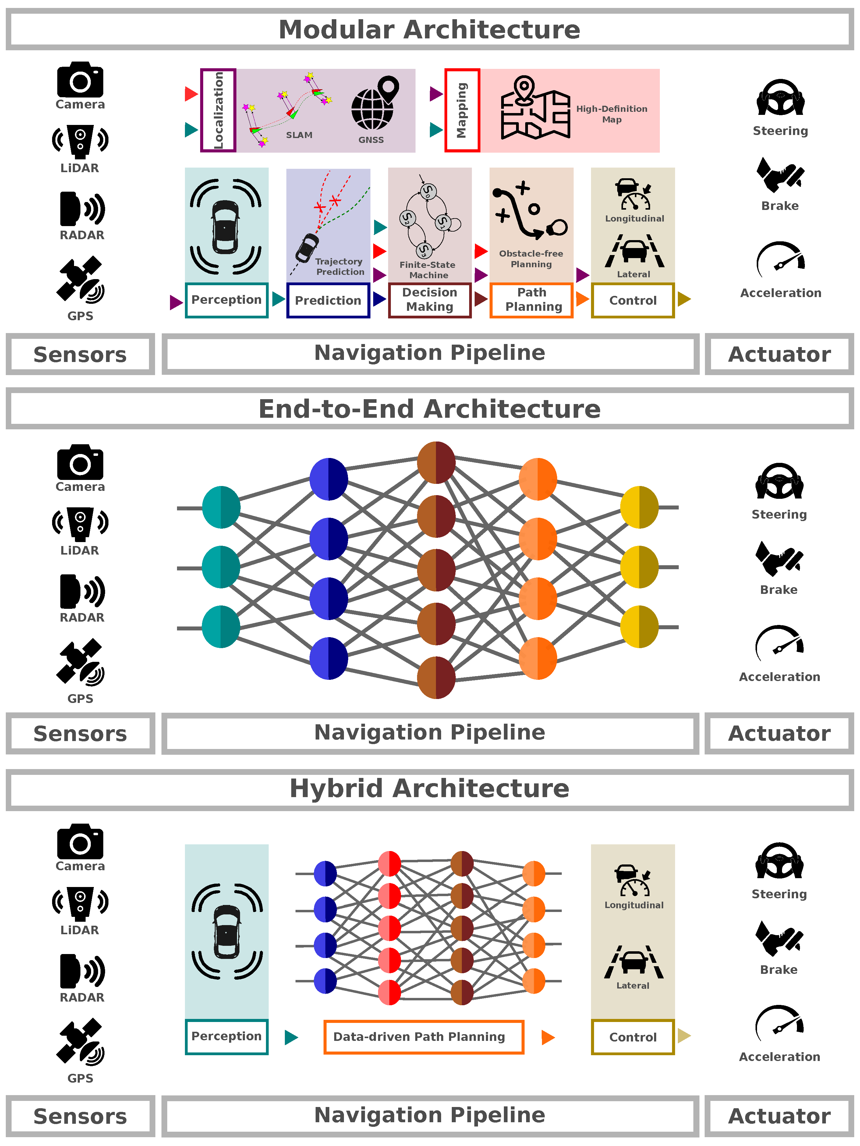
Figure 2.
General design of the proposed Modular architecture.
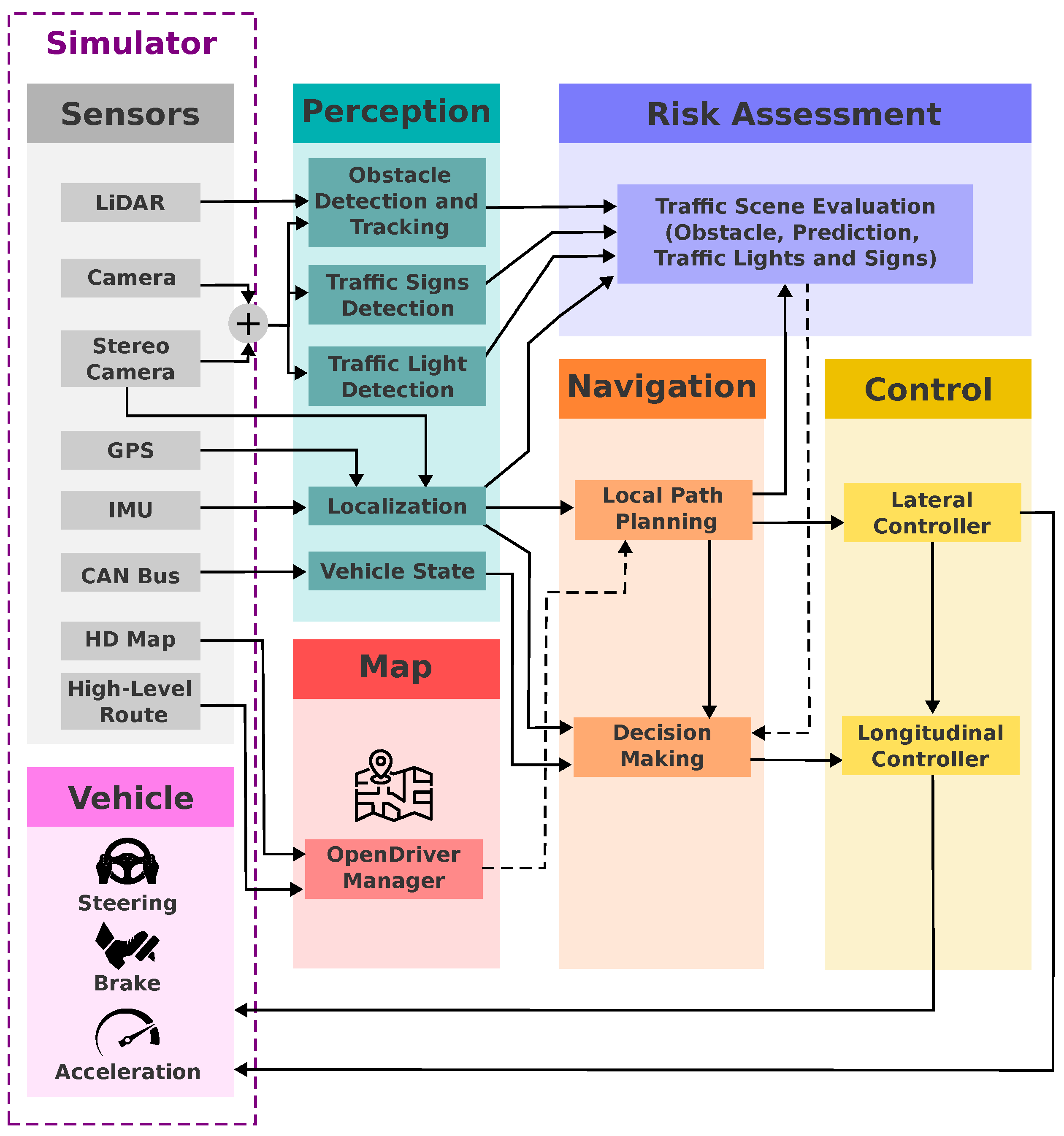
Figure 3.
OpenDRIVE Map. The dots represents high-level commands with red (turn left), blue (turn right), green (keep lane), and white (go-straight).
Figure 3.
OpenDRIVE Map. The dots represents high-level commands with red (turn left), blue (turn right), green (keep lane), and white (go-straight).
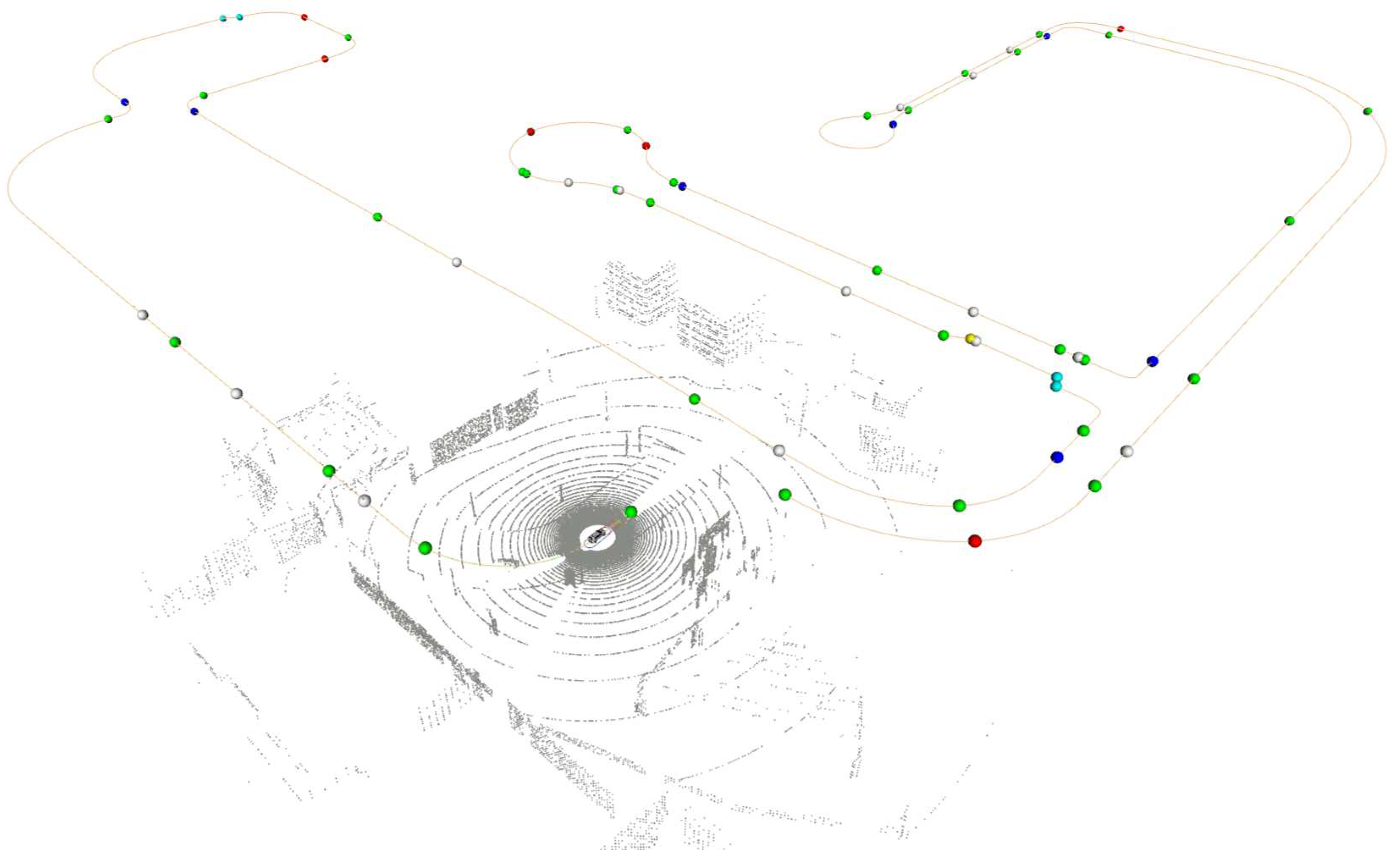
Figure 4.
Perception module.
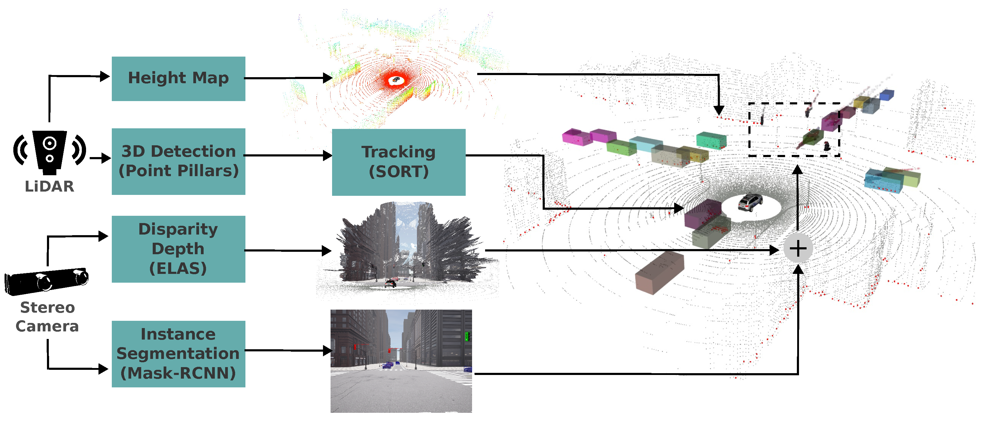
Figure 5.
Risk assessment. Point 1 - Zone of influence of a red traffic light; Point 2 - The predicted trajectory of another car intersects the ego vehicle’s path in the yellow zone; Point 3 - A parked car within the yellow zone is identified as a potential obstacle but receives lower priority compared to threats in the red zone.
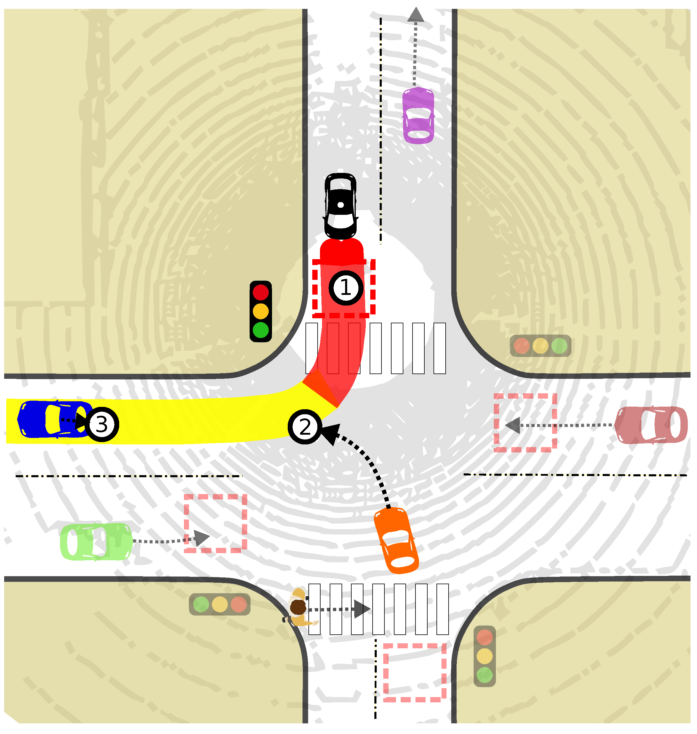
Figure 6.
State transition diagram for the Moore Finite State Machine used in our decision-making module.
Figure 6.
State transition diagram for the Moore Finite State Machine used in our decision-making module.
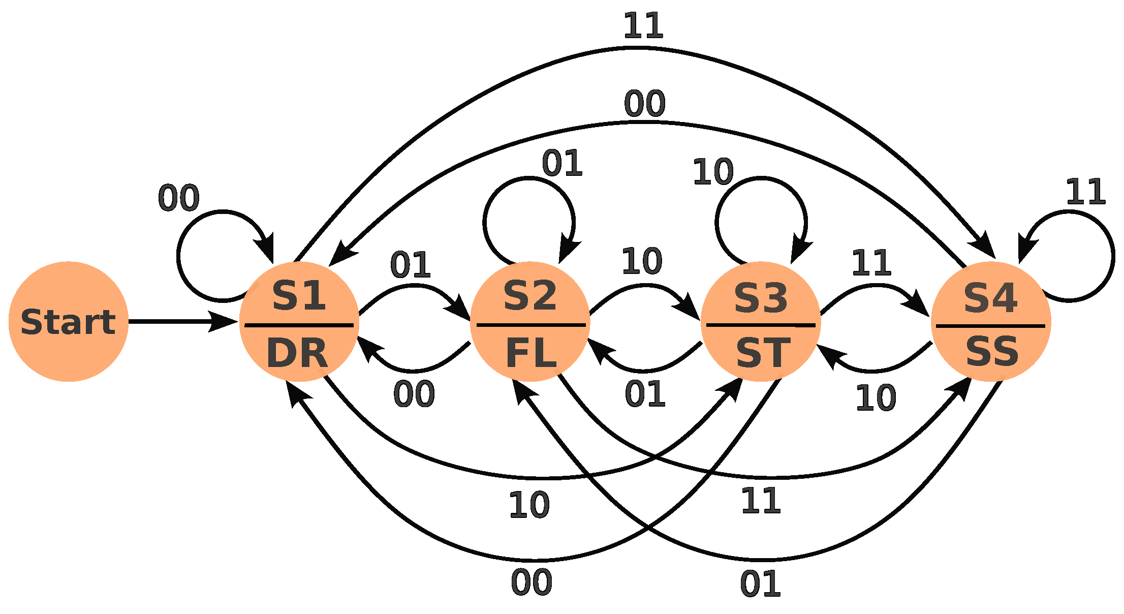
Figure 7.
The pose estimation stack used in our perception module.
Figure 8.
Our neural path planner takes as input BEVSFusion and the output is a list w (path) that is followed by the MPC controller.
Figure 8.
Our neural path planner takes as input BEVSFusion and the output is a list w (path) that is followed by the MPC controller.
Figure 9.
Our instance detection dataset includes annotations of eight classes: Car, pedestrian, bicycle, stop sign, red traffic light, yellow traffic light, green traffic light and emergency vehicle in different urban environments and weather conditions
Figure 9.
Our instance detection dataset includes annotations of eight classes: Car, pedestrian, bicycle, stop sign, red traffic light, yellow traffic light, green traffic light and emergency vehicle in different urban environments and weather conditions
Table 2.
FSM inputs.
| Input | Description |
|---|---|
| 00 | No obstacles detected, indicating a clear path ahead. |
| 01 | An obstacle is being tracked, requiring speed adjustments to maintain safe following distances. |
| 10 | A red traffic light is ahead, necessitating a controlled stop. |
| 11 | A stop sign is detected, also demanding a full stop. |
Table 3.
State transition table (based on hand-crafted rules)
 |
Table 5.
Results: CARLA Leaderboard 1, Track MAP
| Team | Method | DS | RC | IP | CP | CV | CL | RLI | SSI | ORI | RD | RT | AB |
|---|---|---|---|---|---|---|---|---|---|---|---|---|---|
| Anonymous | Map TF++ | 61.17 | 81.81 | 0.70 | 0.01 | 0.99 | 0.00 | 0.08 | 0.00 | 0.00 | 0.00 | 0.00 | 0.55 |
| mmfn | MMFN+(TPlanner)14 | 59.85 | 82.81 | 0.71 | 0.01 | 0.59 | 0.00 | 0.51 | 0.00 | 0.00 | 0.00 | 0.62 | 0.06 |
| LRM 2023 |
CaRINA agent |
41.56 | 86.03 | 0.52 | 0.08 | 0.38 | 0.13 | 1.6 | 0.03 | 0.00 | 0.04 | 0.05 | 1.29 |
| RaphaeL | GRI-based DRL [50] |
33.78 | 57.44 | 0.57 | 0.00 | 3.36 | 0.50 | 0.52 | 0.00 | 1.52 | 1.47 | 0.23 | 0.80 |
| mmfn | MMFN [20] | 22.80 | 47.22 | 0.63 | 0.09 | 0.67 | 0.05 | 1.07 | 0.00 | 0.45 | 0.00 | 0.00 | 1003.88 |
| RobeSafe research group |
Techs4AgeCar+ [51] |
18.75 | 75.11 | 0.28 | 1.52 | 2.37 | 1.27 | 1.22 | 0.00 | 0.59 | 0.17 | 0.01 | 1.28 |
| ERDOS | Pylot [52] | 16.70 | 48.63 | 0.50 | 1.18 | 0.79 | 0.01 | 0.95 | 0.00 | 0.01 | 0.44 | 0.10 | 3.30 |
| LRM 2019 | CaRINA [10] | 15.55 | 40.63 | 0.47 | 1.06 | 3.35 | 1.79 | 0.28 | 0.00 | 3.28 | 0.34 | 0.00 | 7.26 |
Table 6.
Results: CARLA challenge 2023. CARLA leaderboard 2, Track MAP
| Team | Method | DS | RC | IP | CP | CV | CL | RLI | SSI | ORI | RD | RT | AB | YEI | ST | MinSI |
|---|---|---|---|---|---|---|---|---|---|---|---|---|---|---|---|---|
| Kyber-E2E | Kyber-E2E | 3.11 | 5.28 | 0.67 | 0.36 | 0.63 | 0.27 | 0.09 | 0.09 | 0.01 | 0.00 | 0.09 | 0.09 | 0.00 | 0.54 | 0.00 |
| LRM 2023 |
CaRINA agent |
1.14 | 3.65 | 0.46 | 0.00 | 2.89 | 1.31 | 0.00 | 0.53 | 0.00 | 0.13 | 1.31 | 1.18 | 0.00 | 2.10 | 0.00 |
Table 7.
Results: CARLA Leaderboard 1, Track SENSORS
| Team | Method | DS | RC | IP | CP | CV | CL | RLI | SSI | ORI | RD | RT | AB |
|---|---|---|---|---|---|---|---|---|---|---|---|---|---|
| Interfuser | ReasonNet [15] | 79.95 | 89.89 | 0.89 | 0.02 | 0.13 | 0.01 | 0.08 | 0.00 | 0.04 | 0.00 | 0.01 | 0.33 |
| Interfuser | InterFuser [16] | 76.18 | 88.23 | 0.84 | 0.04 | 0.37 | 0.14 | 0.22 | 0.00 | 0.13 | 0.00 | 0.01 | 0.43 |
| PPX | TCP [17] | 75.14 | 85.63 | 0.87 | 0.00 | 0.32 | 0.00 | 0.09 | 0.00 | 0.04 | 0.00 | 0.00 | 0.54 |
| DP | TF++ WP Ensemble [53] |
66.32 | 78.57 | 0.84 | 0.00 | 0.50 | 0.00 | 0.01 | 0.00 | 0.12 | 0.00 | 0.00 | 0.71 |
| WOR | LAV [54] | 61.85 | 94.46 | 0.64 | 0.04 | 0.70 | 0.02 | 0.17 | 0.00 | 0.25 | 0.09 | 0.04 | 0.10 |
| Attention Fields |
TF++ WP [53] | 61.57 | 77.66 | 0.81 | 0.02 | 0.41 | 0.00 | 0.03 | 0.00 | 0.08 | 0.00 | 0.00 | 0.71 |
| DP | TransFuser [55,56] | 61.18 | 86.69 | 0.71 | 0.04 | 0.81 | 0.01 | 0.05 | 0.00 | 0.23 | 0.00 | 0.01 | 0.43 |
| Attention Fields |
Latent TransFuser [55,56] |
45.20 | 66.31 | 0.72 | 0.02 | 1.11 | 0.02 | 0.05 | 0.00 | 0.16 | 0.00 | 0.04 | 1.82 |
| RaphaeL | GRIAD [57] | 36.79 | 61.85 | 0.60 | 0.00 | 2.77 | 0.41 | 0.48 | 0.00 | 1.39 | 1.11 | 0.34 | 0.84 |
| LRM 2023 |
CaRINA hybrid |
35.36 | 85.01 | 0.45 | 0.02 | 4.95 | 0.22 | 1.67 | 0.12 | 0.45 | 1.54 | 0.02 | 0.45 |
| WOR | World on Rails [58] | 31.37 | 57.65 | 0.56 | 0.61 | 1.35 | 1.02 | 0.79 | 0.00 | 0.96 | 1.69 | 0.00 | 0.47 |
| MaRLn | MaRLn [59] | 24.98 | 46.97 | 0.52 | 0.00 | 2.33 | 2.47 | 0.55 | 0.00 | 1.82 | 1.44 | 0.79 | 0.94 |
| Attention Fields |
NEAT [60] | 21.83 | 41.71 | 0.65 | 0.04 | 0.74 | 0.62 | 0.70 | 0.00 | 2.68 | 0.00 | 0.00 | 5.22 |
| SDV | AIM-MT [60] | 19.38 | 67.02 | 0.39 | 0.18 | 1.53 | 0.12 | 1.55 | 0.00 | 0.35 | 0.00 | 0.01 | 2.11 |
| SDV | TransFuser (CVPR 2021) [61] |
16.93 | 51.82 | 0.42 | 0.91 | 1.09 | 0.19 | 1.26 | 0.00 | 0.57 | 0.00 | 0.01 | 1.96 |
| LRM-B | CNN-Planner [62] | 15.40 | 50.05 | 0.41 | 0.08 | 4.67 | 0.42 | 0.35 | 0.00 | 2.78 | 0.12 | 0.00 | 4.63 |
| LBC | Learning by Cheating[63] |
8.94 | 17.54 | 0.73 | 0.00 | 0.40 | 1.16 | 0.71 | 0.00 | 1.52 | 0.03 | 0.00 | 4.69 |
| MaRLn | MaRLn [59] | 5.56 | 24.72 | 0.36 | 0.77 | 3.25 | 13.23 | 0.85 | 0.00 | 10.73 | 2.97 | 0.06 | 11.41 |
| Attention Fields | CILRS [64] | 5.37 | 14.40 | 0.55 | 2.69 | 1.48 | 2.35 | 1.62 | 0.00 | 4.55 | 4.14 | 0.00 | 4.28 |
| LRM 2019 | CaRINA [10] | 4.56 | 23.80 | 0.41 | 0.01 | 7.56 | 51.52 | 20.64 | 0.00 | 14.32 | 0.00 | 0.00 | 10055.99 |
Table 8.
Results: CARLA challenge 2023. CARLA leaderboard 2, Track SENSORS
| Team | Method | DS | RC | IP | CP | CV | CL | RLI | SSI | ORI | RD | RT | AB | YEI | ST | MinSI |
|---|---|---|---|---|---|---|---|---|---|---|---|---|---|---|---|---|
| LRM 2023 |
CaRINA hybrid |
1.23 | 9.55 | 0.31 | 0.25 | 1.64 | 0.25 | 0.25 | 0.40 | 0.43 | 0.10 | 0.30 | 0.60 | 0.10 | 1.20 | 0.15 |
| Tuebingen_AI | Zero-shot TF++ [53] |
0.58 | 8.53 | 0.38 | 0.17 | 1.80 | 0.51 | 0.00 | 3.76 | 0.35 | 0.06 | 0.56 | 0.51 | 0.00 | 2.19 | 0.17 |
| CARLA | baseline | 0.25 | 15.20 | 0.10 | 1.23 | 2.49 | 0.79 | 0.03 | 0.94 | 0.47 | 0.50 | 0.00 | 0.13 | 0.13 | 0.69 | 0.19 |
Disclaimer/Publisher’s Note: The statements, opinions and data contained in all publications are solely those of the individual author(s) and contributor(s) and not of MDPI and/or the editor(s). MDPI and/or the editor(s) disclaim responsibility for any injury to people or property resulting from any ideas, methods, instructions or products referred to in the content. |
© 2024 by the authors. Licensee MDPI, Basel, Switzerland. This article is an open access article distributed under the terms and conditions of the Creative Commons Attribution (CC BY) license (http://creativecommons.org/licenses/by/4.0/).
Copyright: This open access article is published under a Creative Commons CC BY 4.0 license, which permit the free download, distribution, and reuse, provided that the author and preprint are cited in any reuse.


