Preprint
Article

Fuzzy Modeling Framework Using Sector Non-Linearity Techniques for Fixed-Wing Aircrafts

Altmetrics

Downloads

82

Views

21

Comments

0

A peer-reviewed article of this preprint also exists.

Submitted:

31 January 2024

Posted:

01 February 2024

You are already at the latest version

Alerts
Abstract
This paper presents a mathematical modeling approach utilizing a fuzzy modeling framework for fixed wing aircraft systems with the goal of creating a highly desirable mathematical representation for model-based control design applications. The starting point is a mathematical model comprised of fifteen non-linear ordinary differential equations representing the dynamic and kinematic behavior applicable to a wide range of fixed wing aircraft systems. Here the proposed mathematical modeling framework is applied to the AIRBUS A310 model developed by ONERA. The proposed fuzzy modeling framework takes advantage of sector non-linearity techniquesto recast all the non-linear terms from the original model to a set of combined fuzzy rules. The result of this fuzzification is a more suitable mathematical description from the control system design point of view. Therefore, the combination of this fuzzy model and the wide range of control techniques available in the literature for such kind of models will enable us to avoid common control design methods, such as gain scheduling, where stability issues can be extremely challenging.
Keywords: 
Subject: Engineering  -   Control and Systems Engineering

1. Introduction

Piloting a modern aircraft – including crewed, remotely piloted, and fully-autonomous – relies on automatic control systems to insure robust stability and high performance under a wide variety of conditions. Robust stability, often measured by phase and gain margin, is a closed-loop concept that quantifies the ability of a feedback control system to remain stable in the presence of uncertainties, both in the mathematical model as well as unexpected changes in the external environmental conditions. The level of performance required is application specific and is often measured in terms of rise time, overshoots, settling time, and other time-domain performances. Many phases of flight, such as final approach with autonomous landing, require that many variables representing the aircraft attitude state (e.g., aircraft body reference frame relative to a ground reference frame) and translational (e.g., position and velocity relative to the ground) are controlled simultaneously. The level of complexity of any model-based control system design process coupled with the ability to guarantee robust stability and the requisite closed-loop performance depends on an accurate mathematical aircraft model describing both the translational motion as well as the orientation. In general, the more closely the mathematical model reflects the specific aircraft and the environment it flies in (that is, the real-world), the better the actively controlled closed loop system performance is likely to be. Improvements in control system design methodologies stemming from the availability of accurate, yet tractable, mathematical models when combined with effective navigation systems directly contributes to safe, high-performance flight.
The classical mathematical model of the aircraft translation and orientation is comprised of fifteen non-linear differential equations [1]. Many control system design methodologies employ linearized mathematical models based on Taylor series approximation of the fifteen non-linear differential equations about an equilibrium point representing a flight regime of interest. For example, it is a well-known and often studied problem of providing smooth flight of passenger aircraft in the presence of wind turbulence. The mathematical model can be linearized about a wings-level, constant velocity flight condition and the feedback control system design based on linear mathematical models strives to keep the flight smooth and near that equilibrium condition. Large deviations from the equilibrium condition, say due an unexpected large wind shear, can move the aircraft out of the linear region and potentially lead to performance and stability issues. In a single flight, there are many flight regimes from take-off to landing represented by different equilibrium points. One of the extended solutions for this issue is the combination of different controllers with the same structure (i.e. gain scheduling) [2].
This paper presents dynamical models for aircraft control design which implies accurate models with suitable structures for optimizing the control design stage. One of the aims of this paper is present a general modeling framework based on fuzzy logics for control design rather than linearization around various equilibrium points. This work explores fuzzy models with non-linear sector approach due to its proven ability to describe dynamic behavior in the field of non-linear systems (page 6 of [3,4,5,6]).
The application of Fuzzy Logic in the field of aerospace applications has been inherent to the emergence of the first contributions in this area, as shown in [7,8,9]. These earlier works explored the use of fuzzy logic as alternatives in control algorithms, states estimation or fault detection. Afterwards, several contributions have been presented where experimental data and clustering techniques have been combined, together with fuzzy logic for the identification of dynamic models (black-box type) and/or controllers, some of these are [10,11,12].
Since the use of fuzzy logic has given satisfactory results almost from its first applications, it has been widely used in many different areas of the aerospace sector such as dynamic control in hypersonic aircraft surfaces [13], health monitoring for aircraft engines [14], autopilots for helicopters [15] or soft-sensors for Angle-of-Attack (AoA) estimation [16,17]. Furthermore, the application of fuzzy logic in novel areas of the aerospace sector, such as Unmanned Aerial Vehicles (UAVs) or Autonomous Underwater Vehicles (AUVs), is also currently an area of interest, as shown in [18,19,20,21,22,23].
The approach presented in this work is to define a global non-linear fuzzy model representing the global aircraft dynamics. In general, there are two approaches for constructing fuzzy models, (i) identification using input-output data (as mentioned before [10,11,12,24], and (ii) derivation from given non-linear system equations. The proposed fuzzy modeling framework is focused on the second approach and uses the idea of Sector Non-Linearity. This method was introduced by Tanaka & Wang in (page 10 of [3]) and enables the formulation of an equivalent fuzzy model from an original non-linear system using linear subsystems. This approach has been addressed previously in the aerospace field, as shown for example in [23,25,26].
Sector non-linearity technique is based on representing any static non-linear term k ( t ) of a model with a fuzzy quantity which j-th rule is of the form:
IF  z n 1 ( t ) is M z n 1 i n 1 and ... and z n s ( t ) is M z n s i n s
THEN k ( t ) = A k j ( t ) j = 1 , . . . , 2 s j = i n 1 + i n 2 · 2 1 + + i n s · 2 s 1 , i n h { 1 , 2 } h = 1 , . . . , s ,
where z n h ( t ) are the premise variables, and A k j ( t ) are constant values (zero order model) or linear functions depending on the state variables x ( t ) (first order model) of non-linear models.
In this paper, the main objective is to present a new version of the conventional fixed-wing aircraft dynamic model that uses fuzzy logic methods. In particular, a way to obtain an equivalent and complete fuzzy model of such non-linear model. This is the main contribution of this work and distinguishes it from other contributions such as [25,26], where the dynamics of the aircraft are only partially described (longitudinal model), the rotation matrices between the different axes are not included and simplifications are made through the application of Taylor Series to make the problem more affordable. For all these reasons, this article proposes a much more general framework that allows to obtain a global and complete model with a higher accuracy.
Finally, in a future research a Takagi-Sugeno fuzzy model (page 6 of [3]) will developed starting from the fuzzy model obtained in this manuscript. This Takagi-Sugeno model will be used to design non-linear TS fuzzy controllers. On the hand, for a better understanding, the validation and examples of the proposed fuzzy modelling are performed using parameters of an Airbus A310 aircraft [27].
This paper is organized as follows. In Section 2 the classical aircraft dynamic model is presented where the attitude dynamics is represented by quaternions. Section 3 introduces the sector nonl-inearity technique for fuzzy modeling. Section 4 provides the construction of the fuzzy model by selecting model limits and applying these in the dynamic model. Section 5 presents simulation results and validation with the Onera non-linear model benchmark of the A310 [27]. Section 6 offers the conclusions.

2. Classic Aircraft Model with Quaternions

2.1. Quaternions in aircraft dynamic models

It is common to use Euler angles to represent aircraft orientation. They have a very physical interpretation more readily enabling visualization of orientation by humans. However, when utilizing Euler angles it is possible to experience the so-called gimbal lock. For example, if using a roll-pitch-yaw description of the orientation, gimbal lock is a numerical condition that occurs when the pitch angle is ±90°. A potential solution therefore is to represent the orientation in some other way. Quaternions are widely used as attitude representation parameters for rigid bodies, such as aircraft [28,29]. For the dynamic aircraft models in this paper, quaternions are used to represent the orientation between the various reference frames due to their computational efficiency and excellent numerical properties. Computing Euler angles and associated coordinate transformation matrices to and from quaternions is readily accomplished. The three main reference frames utilized here are the body axis reference frame, the Earth-linked reference frame, and the wind axis reference frame described below. Quaternions are used to represent the orientation of the various Earth-linked vertical reference frames to the aircraft body axis reference frames, as well as the orientation between the aircraft wind axes reference frame and the aircraft body axes reference frame.
Body axis reference frame [ x b , y b , z b ] origin at the center of gravity and fixed to the aircraft structure. The x-axis is the longitudinal aircraft axis in which the positioning direction is forward, the y-axis is perpendicular to the aircraft plane of symmetry positive direction out the right wing, and the z-axis perpendicular to the other two and oriented downward.
Earth-linked axis reference frame [ x v , y v , z v ] moves with the aircraft and its origin is also the center of gravity. The x-axis is oriented to the North, the y-axis to the East and z-axis perpendicular to the other two and oriented downward. The x y plane is parallel to the Earth’s surface.
Wind axis reference frame [ x w , y w , z w ] is a particular body axis frame because the x-axis is aligned with airspeed velocity vector which is always tangent to the trajectory. The y-axis is perpendicular to x-axis in the same plane as x b and y b , and the z-axis is perpendicular to the other two and oriented downward.
To increase the numerical robustness of the aircraft attitude, that is to say, to avoid the so-called gimbal lock, a set of parameters should be formulated using the same reference frame in each equation of aircraft dynamic model. For that reason, it is important to define the quaternion transformation coordinate matrix. The transformation matrix from body axis reference frame to the Earth-linked frame is represented by [28,29]
R b v ( Q ( t ) ) = q 0 2 + q 1 2 q 2 2 q 3 2 2 ( q 1 q 2 q 3 q 0 ) 2 ( q 1 q 3 + q 2 q 0 ) 2 ( q 1 q 2 + q 3 q 0 ) q 0 2 q 1 2 + q 2 2 q 3 2 2 ( q 2 q 3 q 1 q 0 ) 2 ( q 1 q 3 q 2 q 0 ) 2 ( q 2 q 3 + q 1 q 0 ) q 0 2 q 1 2 q 2 2 + q 3 2
where Q ( t ) = [ q 0 , q 1 , q 2 , q 3 ] T is the attitude quaternion and satisfies | | Q ( t ) | | = 1 for all t.The matrix R b v ( Q ( t ) ) is an orthonormal matrix, hence R v b ( Q ( t ) ) = R b v ( Q ( t ) ) T . To visualize the aircraft attitude it is useful to extract the Euler angles from the quaternion. For a roll-pitch-yaw Euler angle sequence, we have [28,29]
Φ = ϕ ( t ) θ ( t ) ψ ( t ) = tan 1 ( 2 ( q 2 q 3 + q 0 q 1 ) q 3 2 q 2 2 q 1 2 + q 0 2 ) sin 1 ( 2 ( q 1 q 3 q 0 q 2 ) ) tan 1 ( 2 . ( q 2 . q 1 + q 0 . q 3 ) q 3 2 q 2 2 + q 1 2 + q 0 2 )
where ϕ , θ and ψ are the roll, pitch, yaw angles formed by the rotations of the x b , y b and z b axis, respectively.
The aircraft dynamic model is given by force, moment, and kinematic equations [1]. The aircraft attitude kinematics are given by
Q ˙ ( t ) = 1 2 T ( Q ( t ) ) Ω ( t )
where
T ( Q ( t ) ) = q 1 q 2 q 3 q 0 q 3 q 2 q 3 q 0 q 1 q 2 q 1 q 0
and Ω ( t ) = [ p ( t ) , q ( t ) , r ( t ) ] T is the aircraft angular velocity vector describing the angular velocity of the body reference frame with respect to the Earth-linked reference frame and represented in the body reference frame.
Here we present useful relationships between the various forms of attitude representation (Euler angles, quaternions, and transformation matrices) and the three key reference frames (body axis reference frame, the Earth-linked reference frame, and the wind axis reference frame). We first consider the attitude representation of the wind axis reference frame to the body-axis reference frame. The angle-of-attack, denoted by α ( t ) , represents rotations around the y-axis and the sideslip angle, denoted by β ( t ) , represents rotations around the z-axis. The transformation matrix from wind-axis reference frame to the body axis reference frame is given by [28]
R w b α ( t ) , β ( t ) = cos α ( t ) cos β ( t ) cos α ( t ) sin β ( t ) sin α ( t ) sin β ( t ) cos β ( t ) 0 sin α ( t ) cos β ( t ) sin α ( t ) sin β ( t ) cos α ( t )
The attitude quaternion that represents the orientation of the wind axis reference frame relative to the body axis reference frame is given by
q w b ( α ^ ( t ) , β ^ ( t ) ) = cos α ^ ( t ) cos β ^ ( t ) sin α ^ ( t ) sin β ^ ( t ) cos β ^ ( t ) sin α ^ ( t ) cos α ^ ( t ) sin β ^ ( t )
where we define the half-angles α ^ ( t ) : = α ( t ) / 2 and β ^ ( t ) : = β ( t ) / 2 . Let q w b = q 0 q 1 q 2 q 3 T R 4 . Then the transformation matrix from the wind-axis reference frame to the body axis reference frame is given by
R w b ( q w b ) = 1 2 ( q 0 2 + q 1 2 q 2 2 q 3 2 ) q 1 q 2 q 0 q 3 q 1 q 2 + q 0 q 3 1 2 ( q 0 2 q 1 2 + q 2 2 q 3 2 ) q 0 q 2 q 1 q 3 2 q 2 q 3 q 0 q 2 q 1 q 3 0 1 2 ( q 0 2 q 1 2 q 2 2 + q 3 2 )

2.2. Aircraft dynamic model

The mathematical model describing the translation and orientation of a fixed wing aircraft may be summarized as follows [1]
V ˙ ( t ) = 1 m F ( t ) Ω ( t ) × V ( t ) Ω ˙ ( t ) = I 1 ( M ( t ) Ω ( t ) × I Ω ( t ) ) Q ˙ ( t ) = 1 2 T ( Q ( t ) ) Ω ( t ) X ˙ ( t ) = R b v ( Q ( t ) ) V ( t )
where m is the total mass of the system, V ( t ) = [ u ( t ) , v ( t ) , w ( t ) ] T is the translational velocity in the body reference frame, Ω ( t ) = ( p ( t ) , q ( t ) , r ( t ) ) is the angular velocity represented in the body axis reference frame, X ( t ) is the translational position of the aircraft in the Earth linked reference frame, I is the inertia matrix where I x x , I y y , I z z are the moments of inertia and I x z is a product of inertia. The products of inertia I x y and I y z related to the longitudinal plane ( Y b = 0 ) are both neglected because of the aircraft’s symmetry with respect to this plane. The vectors F and M are the aircraft forces and moments, respectively.
Forces and Moments
The forces applied to the aircraft can be decomposed into three components: engines thrust, gravity, and aerodynamic forces. We have F ( t ) = F e n g ( t ) + F g ( t ) + F a ( t ) , all expressed in the body-axis reference frame. It is assumed that the thrust is aligned with the longitudinal axis body x-axis and given by
F e n g ( t ) = T ( t ) 0 0 ,
where T is the total engine thrust. The gravity force, naturally expressed in the Earth-linked axis frame and transformed to the body-axis reference frame, is given by
F g ( t ) = R v b ( Q ( t ) ) 0 0 m g = m g 2 ( q 1 q 3 q 2 q 0 ) 2 ( q 2 q 3 + q 1 q 0 ) q 0 2 q 1 2 q 2 2 + q 3 2
where g is the gravity near the Earth’s surface. The aerodynamic forces are naturally expressed in the wind-axis reference frame and transformed to the body-axis as
F a ( t ) = q d S R w b ( q w b ) C = q d S R w b C X C Y C Z .
The aerodynamic coefficients C X , C Y and C Z are functions of the system variables, q d is the dynamic pressure, and S is the aerodynamic reference area.
The moment about the center of gravity of the aircraft results from the engine and aerodynamic forces. So we have M ( t ) = M e n g + M a . The model is based on the A310 turbofan aircraft. For this reason, it is assumed that there are two engines delivering the same thrust and the distance of the midpoint of the motors to the center of gravity would be null along the y-axis and x-axis. It is assumed that the engines are located below the center of gravity at z e n g . The moment resulting from the thrust is
M e n g ( t ) = G E × F e n g = 0 z e n g · F e n g x ( t ) 0
where G E is the distance between the center of the gravity "G" and the center of the gravity of the engines "E". The aerodynamic moment is composed of two main terms . The first is directly proportional to the moment coefficients C l , C m and C n , that corresponds to roll, pitch and yaw moments, respectively. The second term is the moment resulting from the aerodynamic forces F a ( t ) applied at the aerodynamic center, denoted by A, which may differ from the center of gravity. The total moment equation is given by
M a ( t ) = q d S c ¯ C l C m C n + G A × F a
where, c ¯ is the aerodynamic mean chord and GA is the distance vector between the center of the gravity and the aerodynamic center, where it is assumed that the distance component is only about the x-axis, denoted by x a .
Aircraft aerodynamic model
In the Civilian Aircraft Landing Challenge [27] the aerodynamic coefficients, C L (lift coefficient), C Y (lateral coefficient), and C D (drag coefficient) are given by
C L = C L 0 + C L α α ( t ) + c ¯ V a ( t ) C L q q ( t ) + C L δ e δ e + + C L H e λ L H L G ( t ) C Y = C Y β β ( t ) + C Y r δ r C D = C D 0 + C D α α ( t ) + C D α 2 α ( t ) 2
Similarly, the moment coefficients about the x-, y- and z-axes are given by:
C l = C l β β ( t ) + c ¯ V a ( t ) ( C l p p ( t ) + ( C l r 0 + C l r α α ( t ) ) r ( t ) ) + + C l δ a δ a + C δ r δ r C m = C m 0 + C m α α ( t ) + c ¯ V a ( t ) C m q q ( t ) + C m δ e δ e + + ( C m H 0 + C m H α α ( t ) ) e λ m H L G ( t ) C n = ( C n β 0 + C n β α α ( t ) ) β ( t ) + c ¯ V a ( t ) ( C n r r ( t ) +
+ ( C n p 0 + C n p α α ( t ) ) p ( t ) ) + + C n δ a δ a + C n δ r δ r
Note that for C L and C m equations, the term that depends on the height of the main landing gear above the runway, denoted by H L G ( t ) , describes the ground effect. The terms δ e , δ a and δ r represent the deflections of the control surface of the elevators, ailerons, and rudder respectively. These equations are functions of angular rate variables, p ( t ) , q ( t ) , r ( t ) , the sideslip angle, β ( t ) , the angle-of-attack denoted by , α ( t ) , and the true airspeed denoted by V a ( t ) . The airspeed is affected by wind, denoted W = W x , W y W z T expressed in the Earth-linked axis reference frame. The airspeed V a = V a x ( t ) , V a y ( t ) V a z ( t ) T in the body-axis reference frame is given by
V a = V ( t ) R v b ( Q ) W
The angle of attack α ( t ) and sideslip β ( t ) are computed via
α ( t ) = tan 1 ( V a z ( t ) V a x ( t ) ) a n d β ( t ) = sin 1 ( V a y ( t ) V a ( t ) )
Finally, the relationship between C L , C D and C X , C Z are given by
C X = C D , C Z = C L .

3. Sector Non-linearity

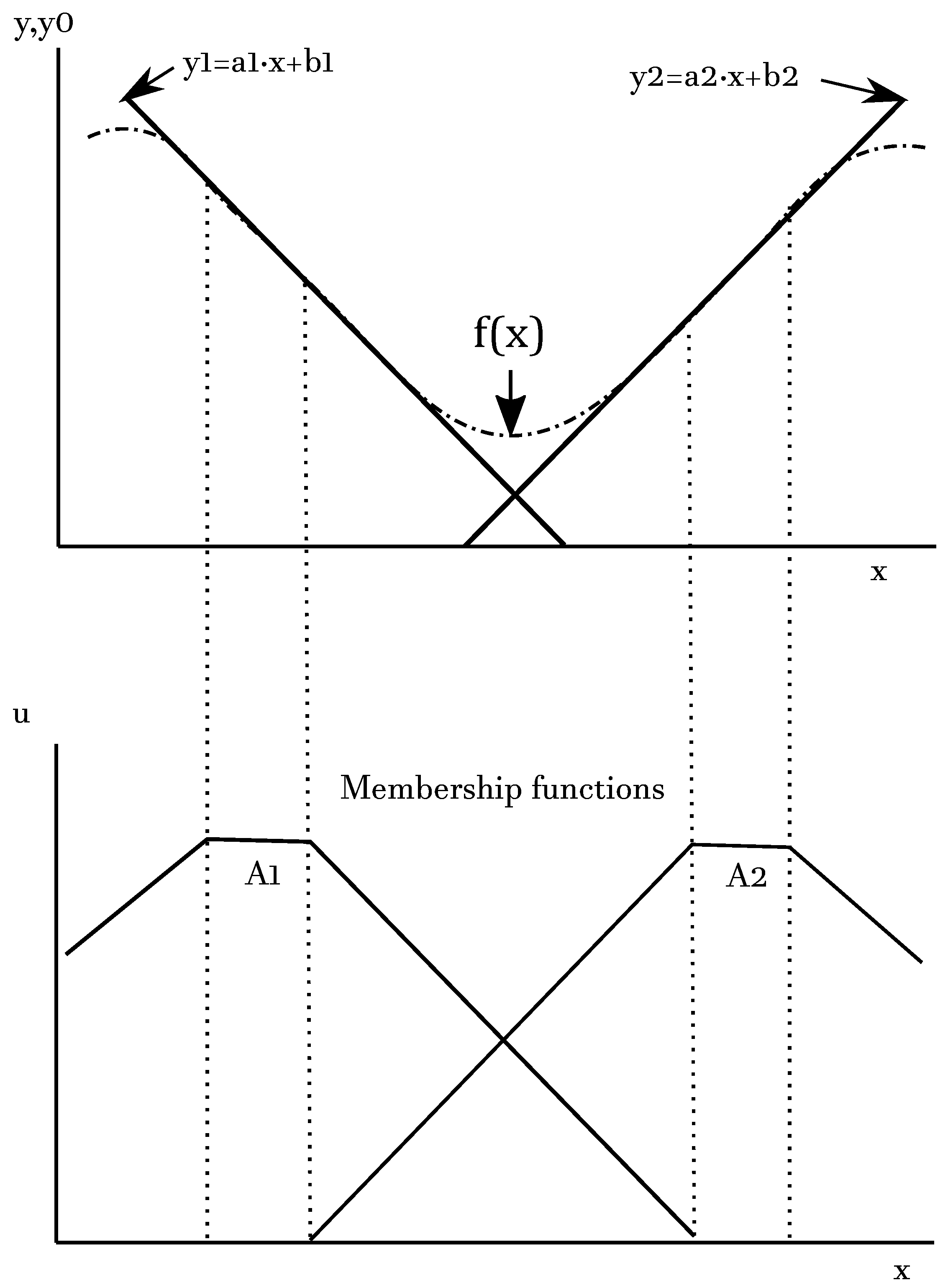
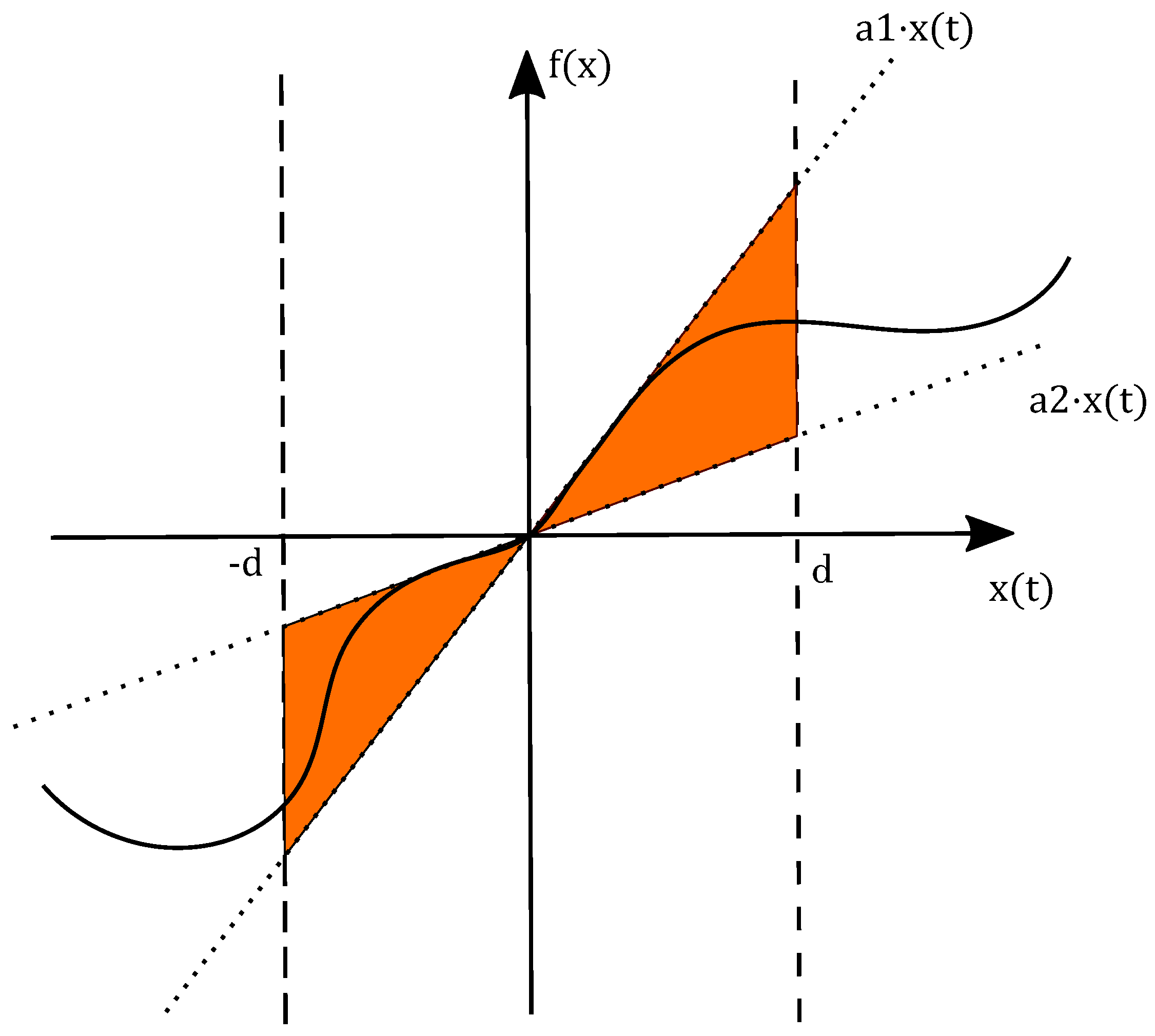
Sector non-linearity in fuzzy model construction appears in page 10 of [3], and is based on the following idea. Consider a non-linear system with a static non-linear term defined by a function f ( x ( t ) ) . The aim is to find the global sector such that f ( x ( t ) ) [ a 1 a 2 ] x ( t ) + [ b 1 b 2 ] . Figure 1 illustrates this approach. Sometimes it is difficult to find global sectors for general non-linear functions. Fortunately, many variables of physical models are easy to bound in aeronautics. In this case, we can consider a local sector non-linearity where two vertical lines become this local sector where d < x ( t ) < d , and where [ d d ] are the limits of the variable x ( t ) as illustrated in Figure 2. It is important to note that for this approach it is necessary that the linear function should intersect the origin of the system. For this paper this would be true for the reason that we are going to apply an equilibrium point.
This approach is going to be used in this paper to obtain the fuzzy representation of static non-linear terms which appear in the non-linear model of fixed wing aircraft according to equation (1).
Example 1: The following non-linear function is the expression of angle-of-attack based on classic aircraft modeling:
α ( t ) = tan 1 x 1 ( t ) x 2 ( t ) = tan 1 ( s ( t ) )
s ( t ) = x 1 ( t ) x 2 ( t )
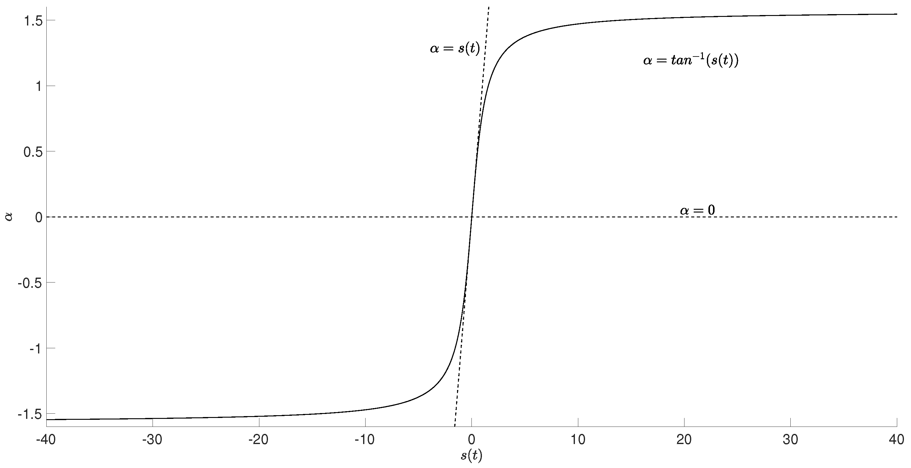
We are going to obtain a fuzzy representation in two steps. In the first step, we deal with the equation between α and s. Figure 3 shows the graphical representation of α ( t ) where two bounds of the global sector might be [ 1 , 0 ] s ( t ) . Therefore, based on these two simple sectors α ( t ) can be represented using (1) with two rules
α ( t ) = M α 1 s ( t ) + M α 2 0
where
M α 1 + M α 2 = 1
The M α 1 and M α 2 consequents are s ( t ) and 0 then:
A α 1 ( t ) = s ( t ) , A α 2 ( t ) = 0
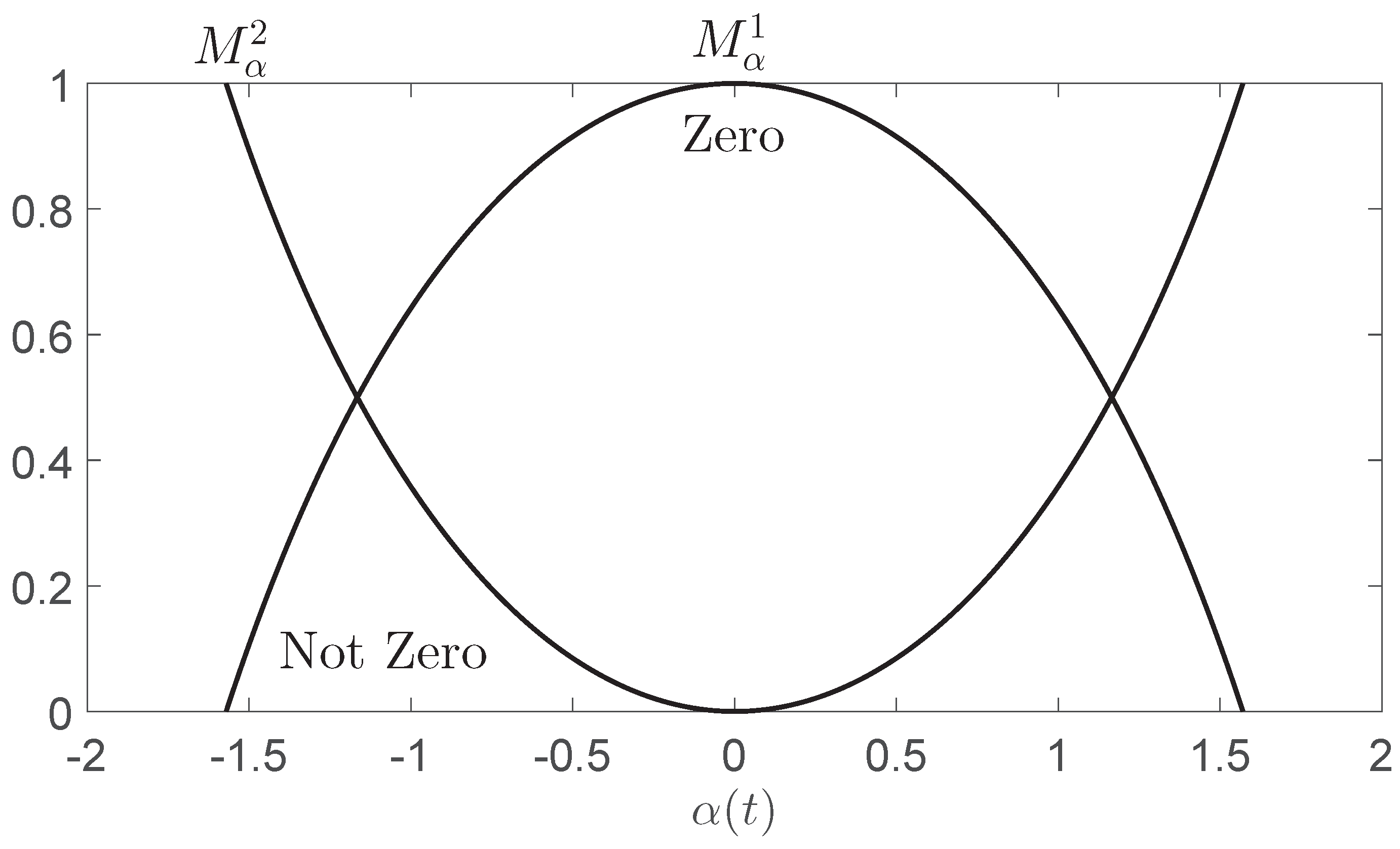
Moreover, α ( t ) is the reference variable of the fuzzy model. Note that the membership function will be dependent on α ( t ) , then it is important to remark that in this function, s ( t ) = tan ( α ( t ) ) . Therefore, the membership functions can be calculated as
M α 1 = α ( t ) t a n ( α ( t ) ) , M α 2 = 1 M α 1 = t a n ( α ( t ) ) α ( t ) t a n ( α ( t ) )
It should be noted that, in general, s 0 , but if this happens, we set M α 1 = 1 and M α 2 = 0 . For the rest of the paper, these membership functions M k i are termed type I.
In the second step we consider s ( t ) . In the angle-of-attack case, s = x 1 x 2 where x 1 ( t ) = V a z ( t ) and x 2 ( t ) = V a x ( t ) . In this non-linear case, the global sector cannot be defined, so a local sector should be used instead, where the quotient is bounded by x 1 x 2 m i n , x 1 x 2 m a x . The reason for these limits is the same as that mentioned at the beginning of Example 1. The outcome of the local sector non-linearity is this fuzzy quantity with two rules
s ( t ) = x 1 ( t ) x 2 ( t ) = N α 1 x 1 x 2 m a x + N α 2 x 1 x 2 m i n
where membership functions are
N α 1 = x 1 ( t ) x 2 ( t ) x 1 x 2 m i n x 1 x 2 m a x x 1 x 2 m i n N α 2 = x 1 x 2 m a x x 1 ( t ) x 2 ( t ) x 1 x 2 m a x x 1 x 2 m i n
In this case, the N α 1 and N α 2 consequents are x 1 x 2 m a x and x 1 x 2 m i n then:
A s 1 ( t ) = x 1 x 2 m a x , A s 2 ( t ) = x 1 x 2 m i n
All membership functions with this structure are defined as type IV and labelled as N k i .
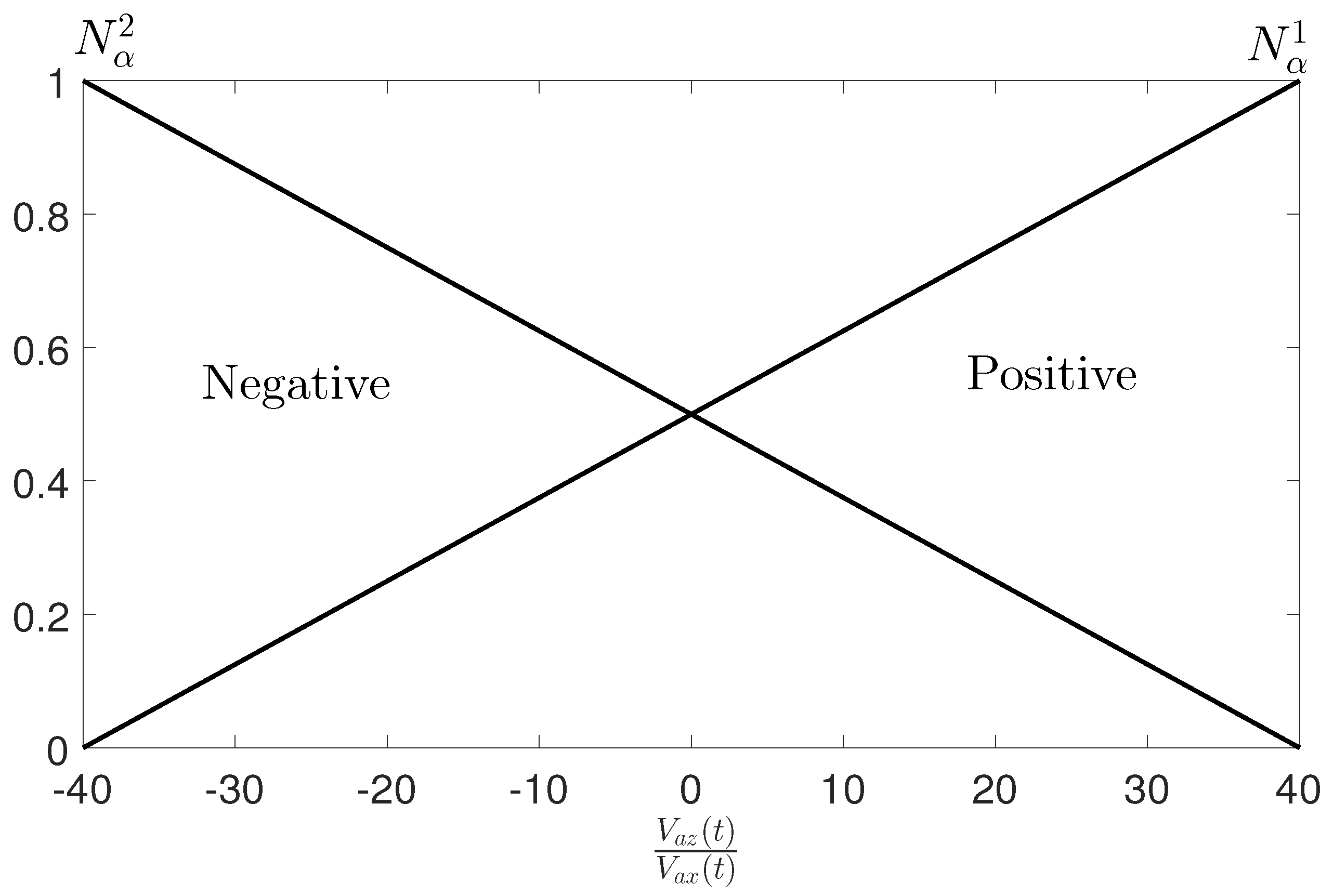
For representing the α ( t ) fuzzy model, the chosen value limits were x 1 x 2 = V a z ( t ) V a x ( t ) [ 40 , 40 ] . In fuzzy models, it is usual to name the membership functions as "Positive", "Negative", "Zero" and "Not Zero" (See Figure 4 and Figure 5). Finally, the fuzzy model for α ( t ) model has four rules after combining fuzzy quantities (22) and (26), and it is presented in Table 1, where
A α 1 = s | s = V a z V a x m a x = 40
A α 2 = s | s = V a z V a x m i n = 40
A α 3 = 0
A α 4 = 0
The defuzzification is carried out as
α ( t ) = j = 1 4 h j A α j
where h 1 = M α 1 N α 1 , h 2 = M α 1 N α 2 , h 3 = M α 2 N α 1 , h 4 = M α 2 N α 2 . This fuzzy model is of zero order because all the consequents are constants.
For further information regarding this example, see example 3 in page 14 of [3].

4. Aircraft Fuzzy Model

As shown in subSection 2.2, there is a large number of non-linear terms associated with aircraft dynamics. As a consequence, these terms are the main objective for applying the sector non-linearity methodology. Here we provide a brief definition of all the types of membership functions and their consequent use following a similar procedure to Example 1 with the membership types I and IV. The different types on membership functions have been chosen on the basis of the different structures of the most repeated non-linear terms.

4.1. Types of membership functions

Example 1 introduces the membership types I and IV, and following the same structure, this section describes types II, III, V, VI and VII.
Type II: β = sin 1 ( x ( t ) )
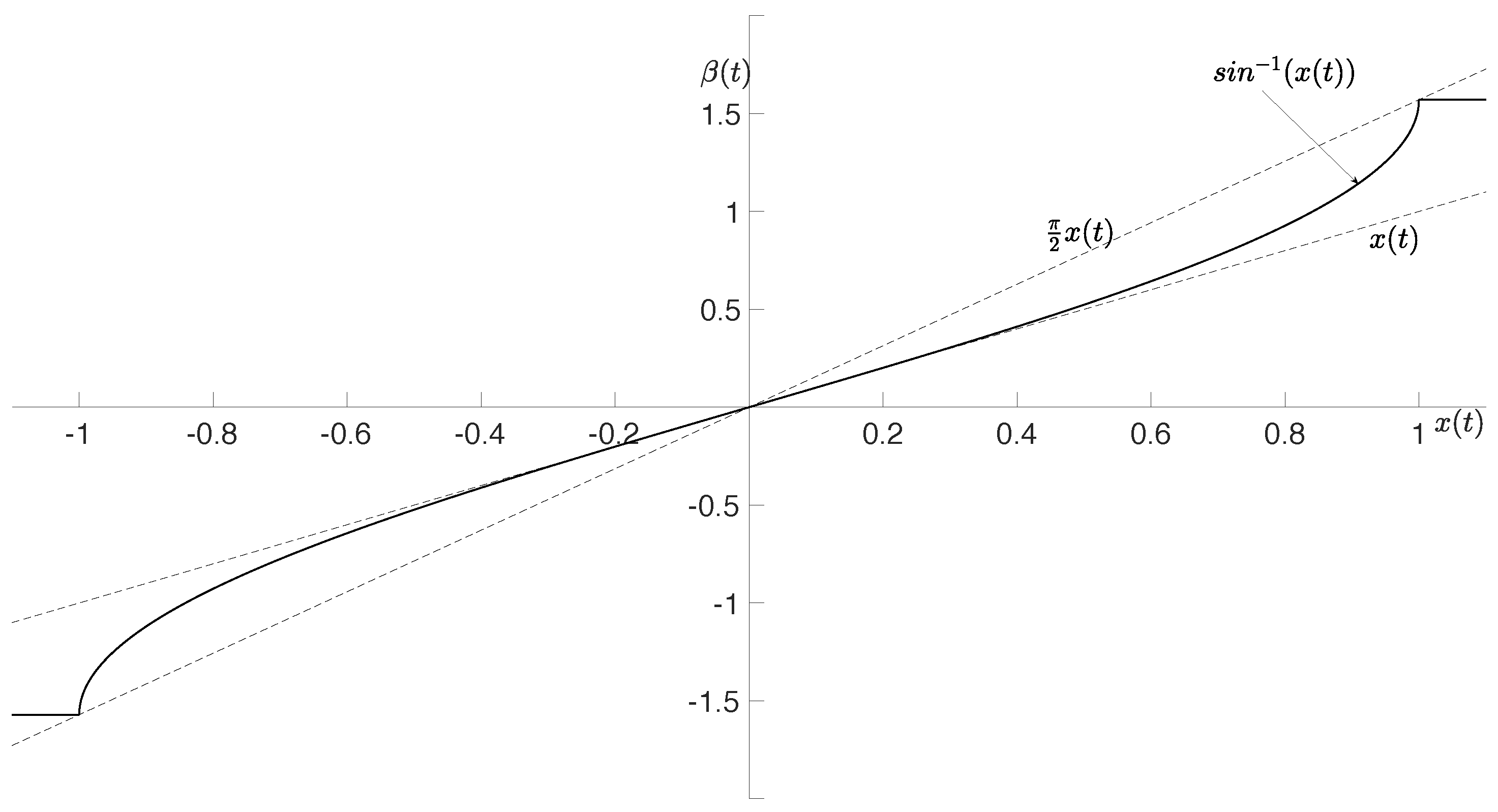
As it can be observed in Figure 6, the function can be delimited by the global sector as β = sin 1 ( x ( t ) ) [ π 2 , 1 ] x ( t ) . The global sector non-linearity method results in the following membership functions of Type II as illustrated in Figure 7:
E β 1 = β ( t ) s i n ( β ( t ) ) s i n ( β ( t ) ) ( π 2 1 ) a n d E β 2 = π 2 s i n ( β ( t ) ) β ( t ) s i n ( β ( t ) ) ( π 2 1 )
Where π 2 x ( t ) and x ( t ) would be their consequents respectively. Consequently, this fuzzy model is of first order.
Type III: z 1 ( t ) = x ( t )
This non-linear term appears in equations (14) and 14. In this particular case, a local sector non-linearity is applied, where bounds are defined as [ x m i n , x m a x ] . Due to the non-negative value for the function, x m i n must be forced to 0. The membership functions can be defined as follows:
F z 1 1 = x ( t ) x m a x a n d F z 1 2 = x m a x x ( t ) x m a x
Where F z 1 1 and F z 1 2 consequents would be x m a x and x m i n = 0 respectively.
Type V: z 2 ( t ) = e x ( t )
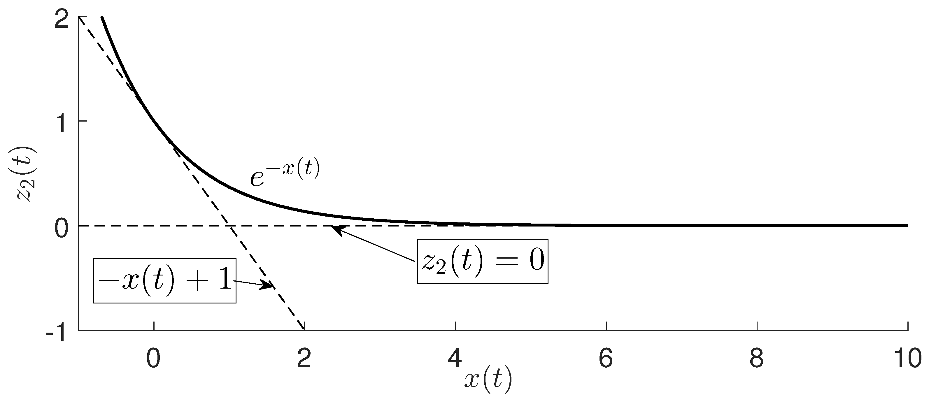
To understand the fuzzy model from this type of equation, consider that the exponential functions are used to model the aircraft ground effect. For this reason, the variable x ( t ) that expresses the distance of the aircraft from the ground, will never be negative. Therefore, the minimum value will be x ( t ) = 0 , giving the maximum of the function z 2 ( t ) = 1 . In consequence, the first local sector is given by x ( t ) + 1 line equation. The other global sector would be defined by its asymptote when x ( t ) reaches high values, and when it is going to be placed at z 2 = 0 . This global sector non-linearity is illustrated in Figure 8. The membership functions of Type V are described in the following equations:
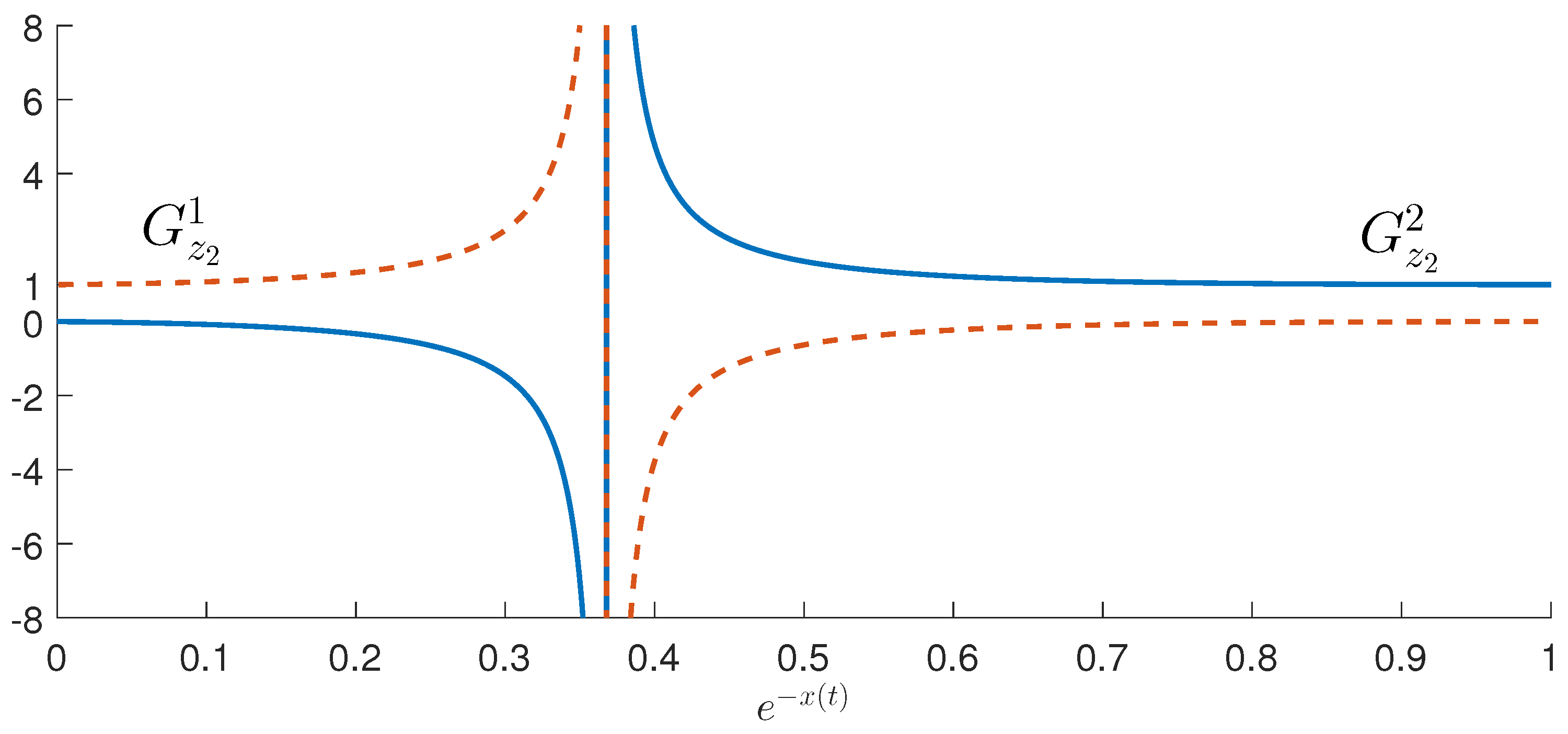
G z 2 1 = e x ( t ) 1 x ( t ) , G z 2 2 = 1 x ( t ) e x ( t ) 1 x ( t )
Where G z 2 1 and G z 2 2 consequent would be 1 x ( t ) and 0 resetroliectively. The membership functions are illustrated in Figure 9.
Particularities of type IV
Example 1 describes the membership function of quotient input terms as x 1 ( t ) x 2 ( t ) . These functions are denoted as N k i and will be used in further membership structures. First, in quadratic terms ( x ( t ) 2 ), where the membership function structure is equivalent to type IV, their consequent would be x m a x and x m i n , respectively. The linear equation terms would also use the N k i form, and its consequents would be a x m a x + b and a x m i n + b respectively. For a better understanding, in the summary Table 2 thru Table 15, the membership function for quadratic terms would be H k i (Type VI) and for liner functions J k i (Type VII).

4.2. Fuzzy application to the aircraft model

Once the different fuzzy model types are defined, the aircraft dynamic model introduced in (8)) to (17) can be reformulated in terms of fuzzy logic. In this new structure, the non-linear terms (except the polynomial forms) can be found in two sets of equations: the wind effects and aerodynamic coefficients.
Wind Effects
The variables included in non-linear terms and related to wind effects are α ( t ) , β ( t ) and V a ( t ) . The fuzzy model of the angle of attack, α ( t ) , is described in Table 1, the fuzzy model of the sideslip angle, β ( t ) , in Table 2, and fuzzy model of the true airspeed, V a ( t ) , in Table 3.
Aerodynamic coefficients
The non-linear terms of the aerodynamic coefficients are reformulated here using the sector non-linearity method. In particular, Equation (28) introduces the non-linear terms C L i , C D i , C l i , C m i and C n i , where i refers the specific coefficient sub-term from the C L , C D , C l , C m and C n aerodynamic coefficients, where
C L 1 = c ¯ V a ( t ) C L q q ( t ) C L 2 = C L H e λ L H L G ( t ) C D 2 = C D α 2 α ( t ) 2 C l 1 = c ¯ V a ( t ) C l p p ( t ) C l 2 = c ¯ V a ( t ) r ( t ) ( C l r 0 + C l r α α ( t ) ) C m 1 = c ¯ V a ( t ) C m q q ( t ) C m 2 = ( C m H 0 + C m H α α ( t ) ) e λ m H L G ( t ) C n 1 = c ¯ V a ( t ) C n r r ( t ) C n 2 = c ¯ V a ( t ) p ( t ) ( C n p 0 + C n p α α ( t ) ) C n 3 = ( C n β 0 + C n β α α ( t ) ) β ( t )
The aerodynamic coefficients in (31) are a combination of different non-linear functions of the types previously described. The fuzzy models of the ten aerodynamic coefficients are described in Table 4, Table 5, Table 6, Table 7, Table 8, Table 9, Table 10, Table 11, Table 12 and Table 13. The maximums and minimums are left as unknown variables where the user should define them. This is because there are different bound conditions for each aircraft type and the objective of this paper is to propose a general model, that is to say, a full flight dynamics model, for later application introducing all the aircraft constants.
In Figure 10 is depicted the procedure to combine all the fuzzy models presented in Table 1, Table 2, Table 3, Table 4, Table 5, Table 6, Table 7, Table 8, Table 9, Table 10, Table 11, Table 12 and Table 13, for obtaining a full fuzzy model for the aircraft.

5. Results and Validation

Due to the complexity of the formulation presented in this work and the large number of fuzzy terms involved, the Fuzzy Modelling Toolbox for Aircraft Systems (FMA Toolbox) has been developed in Matlab. The FMA Toolbox reformulates fixed-wing aircraft models in terms of fuzzy logic, and it can be downloaded at Mathworks File Exchange [30]. Furthermore, to clarify the set of functions and scripts developed in this Toolbox, the detailed user manual can be consulted in [31]. Also, the main implementation of the fuzzy non-linear model for fixed-wing aircrafts can be found in [32], where equations (2)-(17) (introduced in section 2), have been coded in terms of fuzzy logic. This toolbox uses algorithm 1.
Algorithm 1:Aircraft fuzzy model
1:
Set t = 0 . Set initial conditions of the model.
2:
while  t t m a x  do
3:
    Read the values of the inputs at t
4:
    Compute non-linear terms at t using fuzzy models from Table 1, Table 2, Table 3, Table 4, Table 5, Table 6, Table 7, Table 8, Table 9, Table 10, Table 11, Table 12 and Table 13
5:
    Substitute non-linear terms in aircratf model equations (8).
6:
    Integrate these equations and obtain all the states and outputs at t + δ t
7:
    Set t = t + δ t
8:
end while

5.1. Inputs and initial conditions

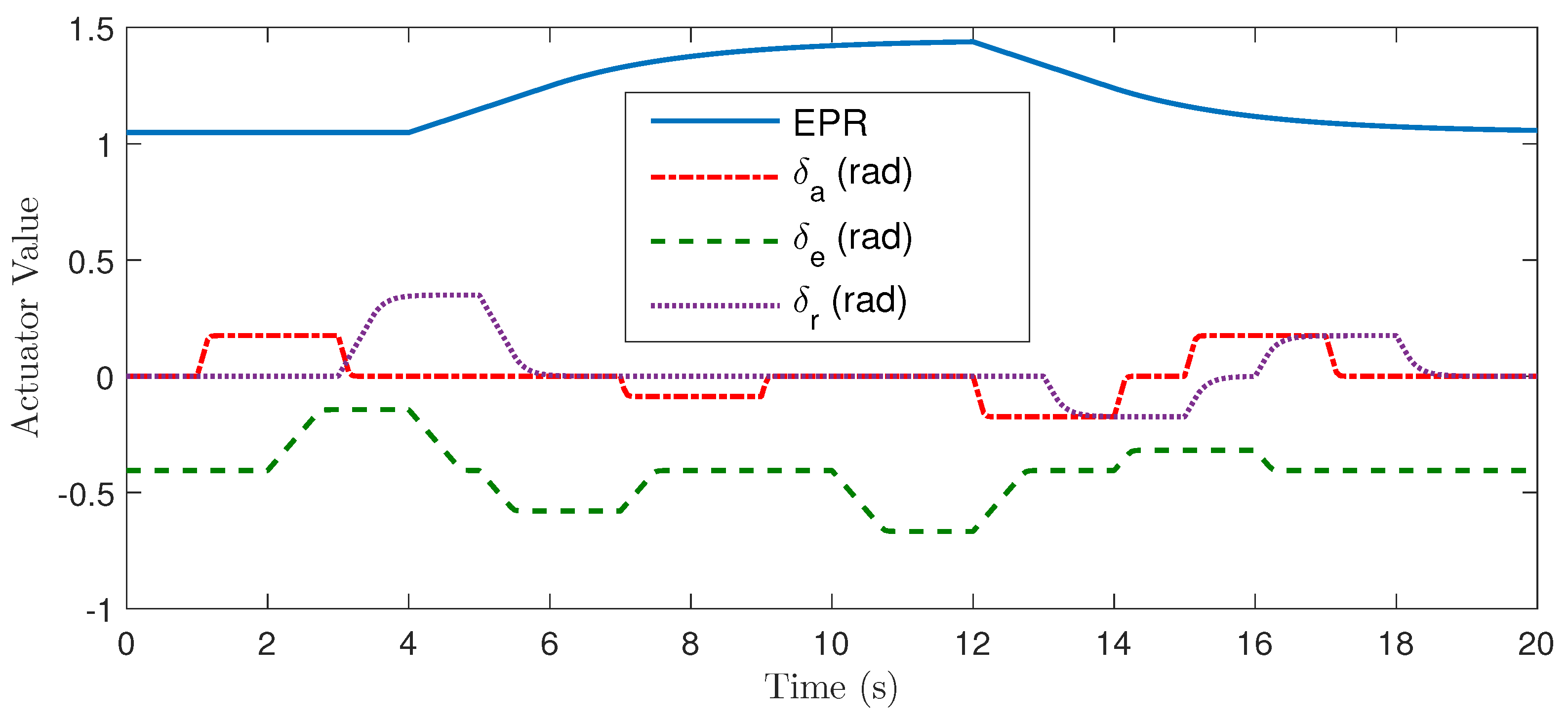
Once the classical aircraft model is completely reformulated in terms of fuzzy logic, it is necessary to test and compare the behavior of these two models using real data. The aircraft dynamic model used here is based on Onera’s benchmark of the landing challenge [27]. Thus it is logical to put the initial values of this model into the fuzzy model. Table 14 shows all the parameters of the Airbus A310 aircraft used here. It should be emphasized that the results are simulated in a short-time frame and that is why the aircraft mass is considered constant, as well as the inertia matrix. The initial conditions of the simulation are calculated as classic Taylor series equilibrium points searching for the actuator trim values. For a more realistic model, these actuators are also modeled and their dynamics are approximated by magnitude and rate limit first-order filters whose characteristics are summarized in Table 15. To obtain significant simulation results, the actuators must vary with different combinations as shown in Figure 11. Finally, the fuzzy model needs maximum and minimum values to be defined. Table 16 defines very conservative limits, for example, α ( t ) and β ( t ) are bounded by a very large interval. Therefore, it is important to remark that some of these value limits can be selected more restrictive, if desired.
Table 14. : Airbus A310 parameters
Mass and Geometry
S=360 m 2 c ¯ = 7.500 m z e n g =2 m m 0 =150000 k g I x x = 10 7 k g / m 2
I y y = 1.600 · 10 7 k g / m 2 I z z = 2.400 · 10 7 k g / m 2 I x z = 10 6 k g / m 2 x C G =21 m
Arodynamic Coefficients
C L 0 = 0.900 C L α = 5.500 C L q = 3.300 C L δ e = 0.320 C L H = 0.200
λ L = 0.120 C D 0 = 0.065 C D α = 0.400 C D α 2 = 1.550 C Y β = 0.700
C Y δ r = 0.250 C l β = 3 C l p = 15 C l r 0 = 5 C l r α = 35
C δ a = 0.700 C l δ r = 0.200 C m 0 = 0.300 C m α = 1.500 C m q = 12
C m δ e = 1.200 C m h 0 = 0.090 C m h α = 0.900 λ m = 0.150 C n β 0 = 0.850
C n β α = 1.950 C n p 0 = 3 C n p α = 35 C n r = 7 C n δ a = 0.04
C n δ r = 1.250
Table 15. : Engine and actuator characteristics
Parameter time-constant lower-bound upper-bound rate-limit
Engines (EPR) 2 s 0.950 1.600 0.100
Ailerons ( δ A ) 0.060 s -55 deg 55 deg 60 deg/s
Elevators ( δ E ) 0.070 s -25 deg 25 deg 20 deg/s
Rudder ( δ R ) 0.200 s -30 deg 30 deg 30 deg/s
Table 16. : Fuzzy model limits
Parameter Lower-Bound Upper-Bound unit
α π 2 π 2 rad
β π 2 π 2 rad
p V a 1 1 rad/m
q V a 1 1 rad/m
r V a 1 1 rad/m
V a 2 1 500 m 2 / s 2
V a z V a x 40 40 (-)
V a y V a 1 1 (-)
H L G 0 40 m

5.2. Simulation results

To compare the non-linear dynamic model of Civilian Aircraft Landing Challenge [27] and the fuzzy logic model, both models have been simulated under equivalent conditions. Particularly, simulations have been carried out using the Toolbox developed in [30]. These simulations have been executed on a PC with Intel Core i5 CPU at 1.6 GHz with 16 GB of DDR3 RAM and using MATLAB 2017B. A computation time of 72 seconds has been necessary to obtain the dynamic evolution of the simulation model for 100 seconds.
On the other hand, the variance accounted for (VAF) index has been used to provide an objective value of the percent of similitude between the two output models. The VAF is governed by the following
V A F i = ( 1 v a r ( y i y ^ i ) v a r ( y i ) ) 100 % ,
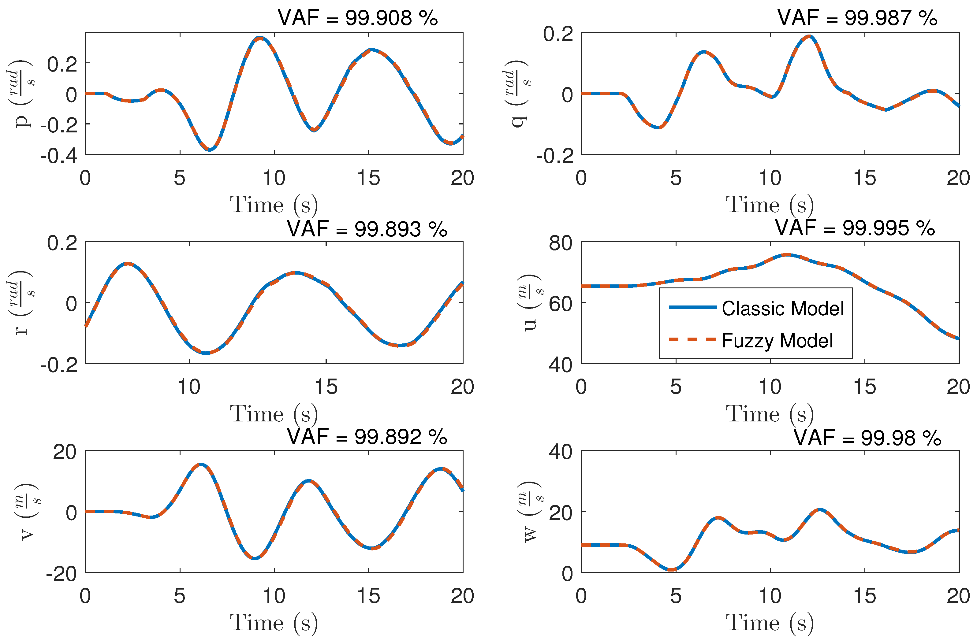
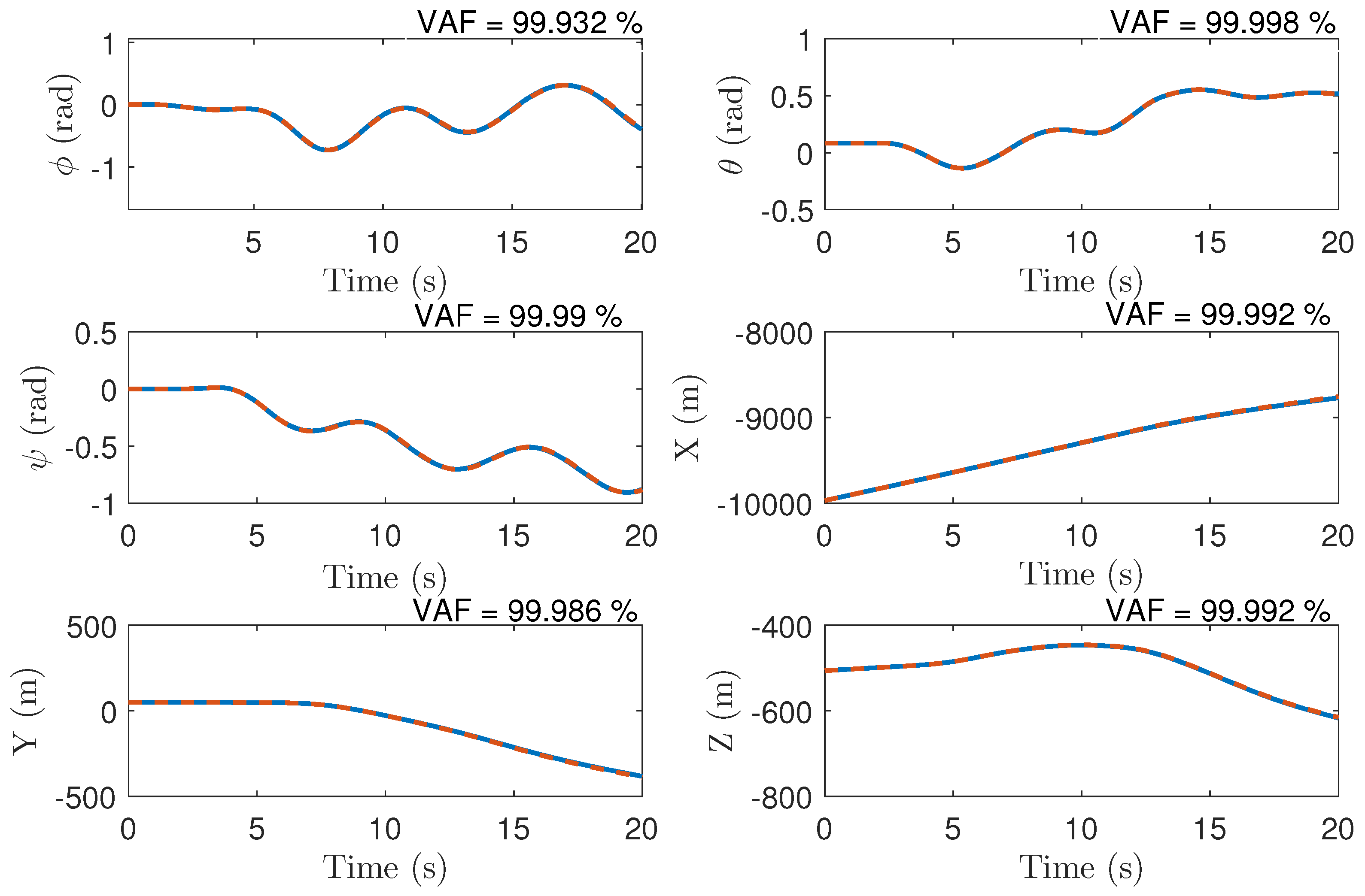
where y i is the measured output (classic model) and y ^ i is the estimated output (fuzzy model) for the i-th component. Figure 12 and Figure 13 show the response of the state variables in both models. Note that the fuzzy modeling method is an exact method, and so the VAFs have high values. Nevertheless, the index is not 100% because the non-linear model of [27] uses the integration of the Euler angles; while this integration is based on quaternions in the fuzzy model. In this simulation, the difference is insignificant due the short period of simulation. Therefore, the error will increase as simulation time increases.

6. Conclusions and Future Works

A general framework for modeling fixed-wing aircraft using fuzzy structures and sector non-linearity techniques has been proposed. The main contribution is to obtain a more general and accurate non-linear model than other alternatives proposed in the existing literature, such as [25,26]. Moreover, the approach presented allows the expression of aerodynamic coefficients, moments, forces and wind effects, all of them expressed in terms of fuzzy logic and respect to the body-frame. This is possible thanks to the capability of the global and local sector non-linearity technique to approximate non-linear terms with fuzzy logic rules and with the same accuracy as the original non-linear model. In addition, the proposed quaternions form has contributed to the good performance of the fuzzy logic model by removing discontinuities and more complex trigonometric functions. However, the good mathematical performance of the quaternions has the negative effect of losing the physical concept of comparing the Euler angles. Nevertheless, it is possible to find an equivalent Euler representation from quaternions.
The main limitation for obtaining the equivalent fuzzy model is the requirement to limit the maximum and minimum values for some of the system variables. This is due to the application of the local sector non-linearity technique, as detailed in sections 3 and 4. However, this limitation is not extremely constraining in the case of fixed-wing aircraft, as there is often a significant amount of information available (theoretical and experimental) from manufacturers and the research community on the limits of these variables.
A Matlab toolbox has been implemented [30] to simplify the application of this new approach for any standard fixed-wing aircraft defined by classical parameters such as geometry, mass, coefficients and bound conditions, where the outcome of the toolbox is a newly reformulated fuzzy model in terms of quaternions.
On the other hand, in section 5 using this Matlab toolbox a fuzzy equivalent model for the Onera non-linear model benchmark of the A310 [27] is obtained. Also, a comparison between the AIR-BUS A310 model developed by ONERA and the obtained fuzzy model is performed. As a consequence, it is concluded that both models are equivalent.
The next step of research consists on obtaining a Takagi-Sugeno fuzzy model (page 6 of [3]) from the fuzzy model obtained in this manuscript. Takagi-Sugeno models are suitable to design non-linear Takagi-Sugeno fuzzy controllers using well known methodologies based on linear matrix inequalities [5,6,33].

Funding

This work has been supported by the Spain goverment via MCIN/AEI/ 10.13039/501100011033 [Project PID2020-119468RA-I00]

Nomenclature

A k j = rule consequent
E k i = type II membership function
F k i = type III membership function
G k i = type V membership function
H k i = type VI membership function
J k i = type VII membership function
M k i = type I membership function
N k i = type IV membership function
i = number of membership function
j = number of rule
k = variable reference of fuzzy model
α = angle of attack, rad
β = aerodynamic sideslip angle, rad
C D , C Y , C L = drag, lateral, and lift force coefficients
C l , C m , C n = roll, pitch and yaw moment coefficients
c ¯ = aerodynamic mean chord, m
δ a , δ e , δ r = ailerons, elevators, and rudder deflections, rad
EPR = exhaust pressure ratio
F = resulting force vector acting on aircraft body, N
F g , F a , F e n g = gravity, aerodynamic, and engine forces, N
F e n g x = x component of the of the engines forces, N
g = gravitational field intensity
near the Earth’s surface, m/ s 2
H L G = landing gear height, m
I = aircraft inertia matrix, k g / m 2
h j = membership function product
I { x x , y y , z z } = moments of inertia on { x b , y b , z b } axes, k g / m 2
I { x y , x z , y z } = products of inertia on { x b , y b , z b } axes, k g / m 2
λ L , λ m = Lift and pitch ground effect coefficients
M = resulting moment vector acting on aircraft body, N.m
m = aircraft total mass, kg
Ω = aircraft angular velocity vector, rad/s
p, q, r = aircraft angular X, Y, and Z velocity components with
respect to ground
and expressed in body axes, rad/s
Φ = euler angles matrix, rad
ϕ, θ, ψ = aircraft Euler angle components, rad
Q = definition of quaternion matrix
q w b = attitude represented from wind axis to body axis
q d = dynamic pressure, k g / ( m . s 2 )
q 0 , q 1 , q 2 , q 3 = quaternion components based on Euler angles
q 0 , q 1 , q 2 , q 3 = quaternion components based on angle of attack and
sideslip angle
R b v = reference system rotation matrix from body axis
to Earth-linked vertical frame
R w b = reference system rotation matrix from wind axis
to body axis
S = principal wing surface, m 2
V = aircraft velocity vector, m/s
V a = true airspeed, m/s
VAF = Variance Accounted For index
u, v, w = aircraft X, Y, and Z velocity components with respect
to ground and expressed in body axes, m/s
x A = X component of aerodynamic aircraft center position, m
x b , y b , z b = components of body axis frame, m
x v , y v , z v = components of earth-linked axis frame, m
x w , y w , z w = components of wind axis frame, m
W = wind velocity vector, m/s
z e n g = Z component of engine gravity center in body axis, m

References

  1. Klein, V.; Morelli, E.A., Aircraft System Identification: Theory and Practice; Sunflyte Enterprises, 2006; chapter 3, pp. 40–42. Section 3.6: Collected Equations of Motion.
  2. Apkarian, P. Advandec Gain-Scheduling Techniques for Uncertain Systems. IEEE Transactions on control systems technology 1998, 6. [Google Scholar] [CrossRef]
  3. Tanaka, K.; Wang, H.O. Fuzzy Control Systems Design and Analysis: A Linear Matrix Inequality Approach; Wiley-Blackwell, 2001. [Google Scholar]
  4. Angelov, P.P.; Filev, D.P. An approach to online identification of Takagi-Sugeno fuzzy models. IEEE Transactions on Systems, Man, and Cybernetics, Part B (Cybernetics) 2004, 34, 484–498. [Google Scholar] [CrossRef] [PubMed]
  5. Wang, H.O.; Li, J.; Niemann, D.; Tanaka, K. TS fuzzy model with linear rule consequence and PDC controller: a universal framework for nonlinear control systems. Ninth IEEE International Conference on Fuzzy Systems. FUZZ-IEEE 2000 (Cat. No. 00CH37063). IEEE, 2000, Vol. 2, pp. 549–554. [CrossRef]
  6. Wang, H.O.; Tanaka, K.; Griffin, M.F. An approach to fuzzy control of nonlinear systems: Stability and design issues. IEEE transactions on fuzzy systems 1996, 4, 14–23. [Google Scholar] [CrossRef]
  7. Larkin, L.I. A fuzzy logic controller for aircraft flight control. The 23rd IEEE Conference on Decision and Control. IEEE, 1984, pp. 894–897. [CrossRef]
  8. Chiu, S.; Chand, S. Fuzzy controller design and stability analysis for an aircraft model. 1991 American Control Conference. IEEE, 1991, pp. 821–826. [CrossRef]
  9. Oosterom, M.; Babuska, R. Virtual sensor for fault detection and isolation in flight control systems-fuzzy modeling approach. Proceedings of the 39th IEEE Conference on Decision and Control (Cat. No. 00CH37187). IEEE, 2000, Vol. 3, pp. 2645–2650. [CrossRef]
  10. Pan, M.; Wang, H.; Huang, J. T–S Fuzzy Modeling for Aircraft Engines: The Clustering and Identification Approach. Energies 2019, 12, 3284. [Google Scholar] [CrossRef]
  11. Weinstein, R.; Hubbard, J.E.; Cunningham, M. Fuzzy modeling and parallel distributed compensation for aircraft flight control from simulated flight data. 2018 Atmospheric Flight Mechanics Conference, 2018, p. 3313. [CrossRef]
  12. Singh, D.J.; Verma, N.K.; Ghosh, A.; Sanwale, J.; Malagaudanavar, A. Aerodynamic Parameter Modeling Using TS Fuzzy Systems from Flight Data. In Computational Intelligence: Theories, Applications and Future Directions-Volume I; Springer, 2019; pp. 425–437. [CrossRef]
  13. Gao, D.; Sun, Z.; Du, T. Dynamic Surface Control of Hypersonic Aircraft Using Fuzzy Logic System. 2007 IEEE International Conference on Automation and Logistics 2007. [Google Scholar] [CrossRef]
  14. Demirci, S.; Hajiyev, C.; Schwenke, A. Fuzzy logic-based automated engine health monitoring for commercial aircraft. Aircraft Engineering and Aerospace Technology 2000, 80, 516–525. [Google Scholar] [CrossRef]
  15. Phillips, C.; Karr, C.L.; Walker, G. Helicopter Flight Control with Fuzzy Logic and Genetic Algorithms. Genetic Algorithms and Fuzzy Logic Systems: Soft Computing Perspectives 1996. [CrossRef]
  16. Singh, D.J.; Dev, R.; Verma, N.K.; Ghosh, A.; Malagaudanavar, A. Estimating angle of attack of an ATAS aircraft using TS fuzzy model. 2017 International Conference on Sensing, Diagnostics, Prognostics, and Control (SDPC). IEEE, 2017, pp. 451–455. [CrossRef]
  17. Singh, D.J.; Agrawal, P.; Verma, N.K.; Ghosh, A.; Malagaudanavar, A. Interval type-2 TS fuzzy model for angle of attack sensor of the aircraft. Journal of Intelligent & Fuzzy Systems 2018, 34, 3891–3901. [Google Scholar] [CrossRef]
  18. Kadmiry, B.; Driankov, D. A fuzzy flight controller combining linguistic and model-based fuzzy control. Fuzzy Sets and Systems 2004, 146, 313–347. [Google Scholar] [CrossRef]
  19. r. Petritoli, E.; Leccese, F., Ed.; Cagnetti, M. Takagi-Sugeno Discrete Fuzzy Modeling: an IoT Controlled ABS for UAV. 2019 II Workshop on Metrology for Industry 4.0 and IoT (MetroInd4.0 IoT), 2019; pp. 191–195. [Google Scholar] [CrossRef]
  20. Mao, X.; Zhang, H.; Wang, Y. Flocking of quad-rotor UAVs with fuzzy control. ISA transactions 2018, 74, 185–193. [Google Scholar] [CrossRef] [PubMed]
  21. Kayacan, E.; Maslim, R. Type-2 fuzzy logic trajectory tracking control of quadrotor VTOL aircraft with elliptic membership functions. IEEE/ASME Transactions on Mechatronics 2016, 22, 339–348. [Google Scholar] [CrossRef]
  22. Rashid, M.; Sheikh, N.; Raza, A.; Raziq, A.; Rehman, A.R.A.; Baber, J.; Basit, A.; others. Development of Dynamic Modeling and Fuzzy Logic System by Classical and Modern Strategies for the Control of Quadcopter. American Scientific Research Journal for Engineering, Technology, and Sciences (ASRJETS) 2019, 62, 108–114. [Google Scholar]
  23. Leccese, F.; Cagnetti, M.; Giarnetti, S.; Petritoli, E.; Luisetto, I.; Tuti, S.; Durovic-Pejcev, R.; Dordevic, T.; Tomašević, A.; Bursić, V.; Arenella, V.; Gabriele, P.; Pecora, A.; Maiolo, L.; De Francesco, E.; Spagnolo, G.S.; Quadarella, R.; Bozzi, L.; Formisano, C. A Simple Takagi-Sugeno Fuzzy Modelling Case Study for an Underwater Glider Control System. 2018 IEEE International Workshop on Metrology for the Sea; Learning to Measure Sea Health Parameters (MetroSea), 2018, pp. 262–267. [CrossRef]
  24. Takagi, T.; Sugeno, M. Fuzzy Identification of Systems and Its Applications to Modeling and Control. IEEE Transactions on systems, man, and cybernetics 1985, SMC-15. [CrossRef]
  25. Hušek, P.; Narenathreyas, K. Aircraft longitudinal motion control based on Takagi–Sugeno fuzzy model. Applied Soft Computing 2016, 49, 269–278. [Google Scholar] [CrossRef]
  26. Tan, B.; Mu, J. Fuzzy Modeling and Control of Longitudinal Channel of F16 Aircraft at a Fixed Speed. 2018 2nd IEEE Advanced Information Management, Communicates, Electronic and Automation Control Conference (IMCEC). IEEE, 2018, pp. 631–636. [CrossRef]
  27. Biannic, J.M.; Boada-Bauxell, J. A Civilian Aircraft Landing Challenge. Onera Benchmark 2016. [Google Scholar]
  28. Diebel, J. Representing Attitude: Euler Angles, Unit Quaternions, and Rotation Vectors. Standford University 2006. [Google Scholar]
  29. Groß ekatthöfer, K.; Yoon, Z. Introduction into quaternions for spacecraft attitude representation. Technical University of Berlin 2012. [Google Scholar]
  30. Brusola, P.; Garcia-Nieto, S. Fuzzy Modelling Toolbox for Aircraft Systems. 2019. Available online: https://es.mathworks.com/matlabcentral/fileexchange/68485-fuzzy-modelling-toolbox-for-aircraft-systems.
  31. Brusola, P.; Garcia-Nieto, S. Fuzzy Modelling Toolbox for Aircraft Systems - User Manual. 2019. Available online: https://github.com/sergarro/fuzzyAircraftModelling/blob/master/Toolbox_Documentation.pdf.
  32. Brusola, P.; Garcia-Nieto, S. Fuzzy Modelling Toolbox for Aircraft Systems - Non-Linear TS Aircraft Model. 2019. Available online: https://github.com/sergarro/fuzzyAircraftModelling/blob/master/src/lib/dFuzzyModeldt.m.
  33. Sala, A.; Ariño, C. Asymptotically necessary and sufficient conditions for stability and performance in fuzzy control: Applications of Polya’s theorem. Fuzzy sets and systems 2007, 158, 2671–2686. [Google Scholar] [CrossRef]
Figure 1. Global sector non-linearity and its membership functions
Preprints 97834 g001
Figure 2. Local sector non-linearity
Preprints 97834 g002
Figure 3. α ( t ) = tan 1 ( s ) global sector non-linearity
Preprints 97834 g003
Figure 4. Membership functions M 1 and M 2 , Type I.
Preprints 97834 g004
Figure 5. Membership functions N 1 and N 2 , Type IV.
Preprints 97834 g005
Figure 6. sin 1 x ( t ) global sector non-linearity
Preprints 97834 g006
Figure 7. sin 1 x ( t ) membership functions
Preprints 97834 g007
Figure 8. e x ( t ) global sector non-linearity
Preprints 97834 g008
Figure 9. G z 2 1 and G z 2 2 membership functions
Preprints 97834 g009
Figure 10. Flowchart which depicts the step by step of modeling process
Preprints 97834 g010
Figure 11. Simulated actuator values
Preprints 97834 g011
Figure 12. Validation of Ω and V
Preprints 97834 g012
Figure 13. Validation of Φ and X
Preprints 97834 g013
Table 1. : α Fuzzy Model
Model Rule 1 Model Rule 2
IF  α ( t ) is "Zero" and IF  α ( t ) is "Zero" and
V a z ( t ) V a x ( t ) is "Positive" V a z ( t ) V a x ( t ) is "Negative"
THEN  α ( t ) = A α 1 THEN  α ( t ) = A α 2
Model Rule 3 Model Rule 4
IF  α ( t ) is "Not zero" and IF  α ( t ) is "Not Zero" and
V a z ( t ) V a x ( t ) is "Positive" V a z ( t ) V a x ( t ) is "Negative"
THEN  α ( t ) = A α 3 THEN  α ( t ) = A α 4
Table 2. : β ( t ) Fuzzy Model
Function: a r c s i n ( V a y ( t ) V a ( t ) ) , Membership function types: II and IV
Max and Min:  ( V a y V a ) m a x = 1 and ( V a y V a ) m i n = 1
Model Rule 1 Model Rule 2
IF  β ( t ) is E β 1 and V a y ( t ) V a ( t ) is N β 1 IF  β ( t ) is E β 1 and V a y ( t ) V a ( t ) is N β 2
THEN  β ( t ) = A β 1 = π 2 THEN  β ( t ) = A β 2 = π 2
Model Rule 3 Model Rule 4
IF  β ( t ) is E β 2 and V a y ( t ) V a ( t ) is N β 1 IF  β ( t ) is E β 2 and V a y ( t ) V a ( t ) is N β 2
THEN  β ( t ) = A β 3 = 1 THEN  β ( t ) = A β 4 = 1
Table 3. : V a ( t ) Fuzzy Model
Function: V a x ( t ) 2 + V a y ( t ) 2 + V a z ( t ) 2 , Membership function types: III
Max and Min:  ( V a x 2 + V a y 2 + V a z 2 ) m a x and ( V a x 2 + V a y 2 + V a z 2 ) m i n = 0
Model Rule 1 Model Rule 2
IF  V a x ( t ) 2 + V a y ( t ) 2 + V a z ( t ) 2 is F V a 1 IF  V a x ( t ) 2 + V a y ( t ) 2 + V a z ( t ) 2 is F V a 2
THEN  V a ( t ) = A V a 1 = ( V a x 2 + V a y 2 + V a z 2 ) m a x THEN  V a ( t ) = A V a 2 = 0
Table 4. : C L 1 Fuzzy Model
Function: C L 1 c ¯ V a ( t ) C L q q ( t ) , Membership function types: IV
Max and Min:  ( q V a ) m a x and ( q V a ) m i n
Model Rule 1 Model Rule 2
IF  q ( t ) V a ( t ) is N C L 1 1 IF  q ( t ) V a ( t ) is N C L 1 2
THEN  C L 1 = A C L 1 1 = c ¯ C L q ( q V a ) m a x THEN  C L 1 = A C L 1 2 = c ¯ C L q ( q V a ) m i n
Table 5. : C L 2 Fuzzy Model
Function: C L 2 = C L H e λ L H L G ( t ) , Membership function types: V
Max and Min:  λ L ( H L G ) m a x and λ L ( H L G ) m i n = 0
Model Rule 1 Model Rule 2
IF  λ L H L G ( t ) is G C L 2 1 IF  λ L H L G ( t ) is G C L 2 2
THEN  C L 2 = A C L 2 1 = C L H ( λ L H L G ( t ) + 1 ) THEN  C L 2 = A C L 2 2 = 0
Table 6. : C D 2 Fuzzy Model
Function: C D 2 = C D α 2 α ( t ) 2 , Membership function types: VI
Max and Min:  α m a x and α m i n
Model Rule 1 Model Rule 2
IF  α ( t ) is H C D 2 1 IF  α ( t ) is H C D 2 2
THEN  C D 2 = A C D 2 1 = C D α 2 α m a x α ( t ) THEN  C L 2 = A C L 2 2 = C D α 2 α m i n α ( t )
Table 7. : C l 1 Fuzzy Model
Function: C l 1 = c ¯ V a ( t ) C l p p ( t ) , Membership function types: IV
Max and Min:  ( p V a ) m a x and ( p V a ) m i n
Model Rule 1 Model Rule 2
IF  p ( t ) V a ( t ) is N C l 1 1 IF  p ( t ) V a ( t ) is N C l 1 2
THEN  C l 1 = A C l 1 1 = c ¯ C l p ( p V a ) m a x THEN  C l 1 = A C L 1 2 = c ¯ C l p ( p V a ) m i n
Table 8. : C l 2 Fuzzy Model
Function: C l 2 = c ¯ V a ( t ) r ( t ) ( C l r 0 + C l r α α ( t ) )
Membership function types: IV and VII
Max and Min:  ( r V a ) m a x and ( r V a ) m i n | α m a x and α m i n
Model Rule 1
IF  r ( t ) V a ( t ) is N C l 2 1 and α ( t ) is J C l 2 1
THEN  C l 2 = A C l 2 1 = ( r V a ) m a x ( C l r 0 + C l r α α m a x )
Model Rule 2
IF  r ( t ) V a ( t ) is N C l 2 1 and α ( t ) is J C l 2 2
THEN  C l 2 = A C l 2 2 = ( r V a ) m a x ( C l r 0 + C l r α α m i n )
Model Rule 3
IF  r ( t ) V a ( t ) is N C l 2 2 and α ( t ) is J C l 2 1
THEN  C l 2 = A C l 2 3 = ( r V a ) m i n ( C l r 0 + C l r α α m a x )
Model Rule 4
IF  r ( t ) V a ( t ) is N C l 2 2 and α ( t ) is J C l 2 2
THEN  C l 2 = A C l 2 4 = ( r V a ) m i n ( C l r 0 + C l r α α m i n )
Table 9. : C m 1 Fuzzy Model
Function: C m 1 = c ¯ V a ( t ) C m q q ( t ) , Membership function types: IV
Max and Min:  ( q V a ) m a x and ( q V a ) m i n
Model Rule 1 Model Rule 2
IF  q ( t ) V a ( t ) is N C m 1 1 IF  q ( t ) V a ( t ) is N C m 1 2
THEN  C m 1 = A C m 1 1 = c ¯ C m q ( q V a ) m a x THEN  C m 1 = A C m 1 2 = c ¯ C m q ( q V a ) m i n
Table 10. : C m 2 Fuzzy Model
Function: C m 2 = ( C m H 0 + C m H α α ( t ) ) e λ m H L G ( t )
Membership function types: V and VII
Max and Min:  λ m H L G , m a x and λ m H L G , m a x | α m a x and α m i n
Model Rule 1
IF  λ m H L G ( t ) is G C m 2 1 and α ( t ) is J C m 2 1
THEN  C m 2 = A C m 2 1 = ( λ m H L G ( t ) + 1 ) ( C m H 0 + C m H α α m a x )
Model Rule 2
IF  λ m H L G ( t ) is G C m 2 1 and α ( t ) is J C m 2 2
THEN  C m 2 = A C m 2 2 = ( λ m H L G ( t ) + 1 ) ( C m H 0 + C m H α α m i n )
Model Rule 3
IF  λ m H L G ( t ) is G C m 2 2 and α ( t ) is J C m 2 1
THEN  C m 2 = A C m 2 3 = 0
Model Rule 4
IF  λ m H L G ( t ) is G C m 2 2 and α ( t ) is J C m 2 2
THEN  C m 2 = A C m 2 4 = 0
Table 11. : C n 1 Fuzzy Model
Function: c ¯ V a ( t ) C n r r ( t ) , Membership function types: IV
Max and Min:  ( r V a ) m a x and ( r V a ) m i n
Model Rule 1 Model Rule 2
IF  r ( t ) V a ( t ) is N C n 1 1 IF  r ( t ) V a ( t ) is N C n 1 2
THEN  C n 1 = A C n 1 1 = c ¯ C n r ( r V a ) m a x THEN  C n 1 = A C n 1 2 = c ¯ C n r ( r V a ) m i n
Table 12. : C n 2 Fuzzy Model
Function: C n 2 = c ¯ V a ( t ) p ( t ) ( C n p 0 + C n p α α ( t ) )
Membership function types: IV and VII
Max and Min:  ( p V a ) m a x and ( p V a ) m i n | α m a x and α m i n
Model Rule 1
IF  p ( t ) V a ( t ) is N C n 2 1 and α ( t ) is J C n 2 1
THEN  C n 2 = A C n 2 1 = ( p V a ) m a x ( C n p 0 + C n p α α m a x )
Model Rule 2
IF  p ( t ) V a ( t ) is N C n 2 1 and α ( t ) is J C n 2 2
THEN  C n 2 = A C n 2 2 = ( p V a ) m a x ( C n p 0 + C n p α α m i n )
Model Rule 3
IF  p ( t ) V a ( t ) is N C n 2 2 and α ( t ) is J C n 2 1
THEN  C n 2 = A C n 2 3 = ( p V a ) m i n ( C n p 0 + C n p α α m a x )
Model Rule 4
IF  p ( t ) V a ( t ) is N C n 2 2 and α ( t ) is J C n 2 2
THEN  C n 2 = A C l 2 4 = ( p V a ) m i n ( C n p 0 + C n p α α m i n )
Table 13. : C n 3 Fuzzy Model
Function: C n 3 = ( C n β 0 + C n β α α ( t ) ) β ( t )
Membership function types: IV and VII
Max and Min:  β m a x and β m i n | α m a x and α m i n
Model Rule 1
IF  β ( t ) is H C n 3 1 and α ( t ) is J C n 3 1
THEN  C n 3 = A C n 3 1 = β m a x ( C n β 0 + C n β α α m a x )
Model Rule 2
IF  β ( t ) is H C n 3 1 and α ( t ) is J C n 3 2
THEN  C n 3 = A C n 3 2 = β m a x ( C n β 0 + C n β α α m i n )
Model Rule 3
IF  β ( t ) is H C n 3 2 and α ( t ) is J C n 3 1
THEN  C n 3 = A C n 3 3 = β m i n ( C n β 0 + C n β α α m a x )
Model Rule 4
IF  β ( t ) is H C n 3 2 and α ( t ) is J C n 3 2
THEN  C n 3 = A C n 3 4 = β m i n ( C n β 0 + C n β α α m i n )
Disclaimer/Publisher’s Note: The statements, opinions and data contained in all publications are solely those of the individual author(s) and contributor(s) and not of MDPI and/or the editor(s). MDPI and/or the editor(s) disclaim responsibility for any injury to people or property resulting from any ideas, methods, instructions or products referred to in the content.
Copyright: This open access article is published under a Creative Commons CC BY 4.0 license, which permit the free download, distribution, and reuse, provided that the author and preprint are cited in any reuse.
Prerpints.org logo

Preprints.org is a free preprint server supported by MDPI in Basel, Switzerland.

Subscribe

© 2024 MDPI (Basel, Switzerland) unless otherwise stated