Submitted:
29 January 2024
Posted:
31 January 2024
You are already at the latest version
Abstract
This study explores the use of Bayesian Neural Networks (BNNs) for estimating chlorophyll-a concentration ([CHL-a]) from remotely sensed data. The BNN model enables uncertainty quantification, offering additional layers of information compared to traditional ocean colour models. An extensive in situ bio-optical dataset is utilized, generated by merging 27 data sources across the world’s oceans. The BNN model demonstrates remarkable capability in capturing mesoscale features and ocean circulation patterns, providing comprehensive insights into spatial and temporal variations in [CHL-a] across diverse marine ecosystems. In comparison to established ocean colour algorithms, such as Ocean Colour 4 (OC4), the BNN shows comparable performance in terms of correlation coefficients, errors, and biases when compared with the in situ data. The BNN, however, further provides critical information about the distribution of [CHL-a], which can be used to assess uncertainties in the prediction. Moreover, the BNN model’s ability to provide more information for coastal waters, especially with higher spatial resolution imagery, offers valuable advantages for marine research and management. By quantifying uncertainty, the model builds confidence in [CHL-a] predictions, even in regions with limited data coverage. This is reflected by the spread in the model predictions, where the BNN can detect a range of uncertainty bounds that reflect confidence in the retrievals. Introducing BNNs as probabilistic ocean colour models represents a significant advancement, enabling more accurate and reliable predictions of [CHL-a] in the global oceans.
Keywords:
Ocean Colour
; Chlorophyll-a
; Remote Sensing
; Bayesian Neural Network
1. Introduction
Phytoplankton are a diverse group of microscopic photosynthetic organisms that play a crucial role in marine ecosystems and global biogeochemical cycles. Functioning as primary producers, they harness solar energy to convert carbon dioxide and nutrients into organic matter, serving as the foundation of the marine food web [1]. Their pivotal role extends to the cycling of carbon, nitrogen, and other elements between the atmosphere and the ocean [2,3]. Phytoplankton also act as climate regulators by absorbing substantial amounts of atmospheric carbon dioxide during photosynthesis, thereby mitigating the impacts of greenhouse gas emissions on the planet’s climate system [4,5,6]. Additionally, they contribute significantly to oxygen production in the ocean, a vital element for the survival of marine organisms [3,7]. Apart from their ecological and biogeochemical importance, changes in phytoplankton phenology can have direct impacts on human societies by influencing the survival of fish larvae and consequently fish stocks [8]. Harmful algal blooms (HABs), for instance, can release toxins that accumulate in seafood, posing threats to human health and causing disruptions in local economies [9]. It is, therefore, important to understand phytoplankton dynamics and identify changes to their seasonality and abundance.
Monitoring phytoplankton through remote sensing is important to study their distribution, abundance, and productivity across the world oceans and inland waters [10]. Remote sensing enables the acquisition of high-resolution data on large spatial and temporal scales, providing a comprehensive understanding of the processes governing phytoplankton dynamics [11]. A key advantage of remote sensing lies in its capacity to offer synoptic coverage of the ocean surface, surpassing the limitations of traditional sampling methods [12]. This facilitates detecting spatial and temporal patterns in phytoplankton abundance and productivity, as well as the identification of ecological hotspots [13] and their responses to global environmental changes, such as oceanic warming, ocean acidification, and eutrophication [14]. Furthermore, monitoring oceans via remote sensing can provide early warnings of HABs, thereby enabling effective mitigation of the associated risks [15,16]. Remotely sensed data can also be utilized to calibrate and validate ocean biogeochemical models, which are crucial for predicting the responses of marine ecosystems to global environmental changes [17].
Ocean colour algorithms are analytical tools that harness satellite imagery to estimate the concentrations of phytoplankton, sediment, and dissolved organic matter in the oceans. These algorithms operate on the principle of light absorption and scattering by various components present in the water, which influence the observed colour of light reflected from the ocean’s surface [18]. To estimate phytoplankton concentration, these algorithms leverage the unique spectral characteristics exhibited by the pigment. Chlorophyll-a, the dominant photosynthetic pigment found in most phytoplankton, displays a distinctive optical signature, with high absorption of blue and red light and relatively high reflection of green light [19,20]. Often utilising the ratio (or difference) in blue to green light reflected by the ocean’s surface, these algorithms can derive estimates of chlorophyll-a concentration ([CHL-a]), thereby inferring the abundance of phytoplankton [18]. Recent advances in satellite technology and algorithm development have significantly improved the accuracy of these empirical algorithms [21,22]. However, the performance of ocean colour models can still vary depending on the studied environmental conditions, with some regions posing greater challenges [21]. Studies evaluating the performance of ocean colour algorithms generally indicate reasonable estimates across a range of conditions, though their accuracy can be affected by factors like cloud cover, atmospheric interference, bottom reflectance, and the presence of other water constituents, for example, in rivers and estuaries [23,24]. Different techniques could provide better solutions to such issues.
Neural networks have emerged as a promising approach for analyzing complex remote sensing data, as they can learn to recognize patterns within the data. One notable example is the Case2R algorithm developed by using the Inverse Modelling Technique [25]. This algorithm uses an Inverse Radiative Transfer Model-Neural Network (IRTM-NN) to estimate [CHL-a] and total suspended matter from normalized water-leaving reflectance, employing a large database of in situ measurements for training and validation [25]. Convolutional Neural Networks (CNN) and Artificial Neural Networks (ANN) have also demonstrated promising results in accurately estimating [CHL-a], with some studies reporting improved accuracy compared to traditional ocean colour algorithms [26,27,28,29]. These methods provide deterministic estimates of [CHL-a] even though the dataset itself is noisy; particularly due to various sources of errors in collecting [CHL-a] samples and imperfect remotely sensed imagery. On the other hand, a branch of deep learning investigates the realm of probabilistic neural network models, which allow for uncertainty quantification and stochastic model evaluation [30].
Bayesian Neural Networks (BNNs) are a class of neural networks that incorporate probabilistic modeling, generally using Bayes’ rule, to capture uncertainty in the model’s predictions [31]. A BNN treats its parameters as random variables by associating a probability distribution to the network’s weights. Training these probabilistic networks involves incorporating prior distributions over the network weights, which are then updated using Bayesian inference techniques, such as Markov Chain Monte Carlo or variational methods [32]. By accounting for uncertainty, BNNs enable more efficient and robust predictions, especially in scenarios with limited data or complex datasets [33]. Bayesian models, including BNNs, offer significant advantages to deterministic models, notably in their capacity to integrate prior knowledge, estimate uncertainties through probability distributions, and exhibit robustness against overfitting due to their probabilistic framework [34]. However, it’s important to note that these benefits come at the cost of increased computational complexity compared to conventional Markov Chain Monte Carlo techniques, necessitating more extensive training time. Nevertheless, these models have found applications in various fields, including but not limited to computer vision [35], natural language processing [36], robotics [37], and healthcare [38], where reliable uncertainty estimates and probabilistic reasoning are essential for making informed decisions and assessing risks.
The application of BNNs in ocean colour remote sensing to address some of the common challenges listed above remains relatively unexplored. It is worth mentioning that Werther et al. 2022 proposes using Monte Carlo dropout as means of achieving a BNN ocean colour model, whereas here, the full posterior distribution of the NN’s parameters is obtained using Bayes rule. Specifically, by relying on Monte Carlo dropout the posterior for the NN parameters they obtain is a probability density function defined by two points, where the parameter assumes the trained value with some set probability p or a value of zero with probability . This is different than inferring the posterior distribution function using Bayes’ rule.
This study introduces a new BNN ocean colour algorithm designed to enhance the estimation of [CHL-a] from remotely sensed reflectance data while providing robust means for uncertainty quantification. The new BNN ocean colour model is applicable at a global scale, and improves upon traditional deterministic models by predicting the probability distribution of [CHL-a]. The aim of this research is to address the limitations of traditional ocean colour algorithms by integrating Bayesian inference principles into the algorithmic framework. The study explores the accuracy and reliability of the BNN ocean colour algorithm through systematic experimentation and comparison with existing algorithms. Specifically, the strength of the proposed methodology lies in the ability to perform a comprehensive statistical analysis with uncertainty quantification estimates. The findings of this study are expected to provide new insights to the field of ocean colour remote sensing and contribute to a deeper understanding of phytoplankton dynamics.
2. Match-up Data
We utilized the extensive bio-optical in situ database from Valente et al. 2022, which merges 27 datasets that were individually processed to maximize data quality. Observations with missing or incorrect date and/or geographic coordinates, as well as those obtained using incompatible measurement methods or exhibiting extreme values were excluded. This comprehensive database was constructed by applying a specified threshold for the coefficient of variation to assess spatial and temporal variability among replicate data points. Observations below this threshold were averaged, while those exceeding it were discarded, thereby ensuring a reliable and consistent dataset.
The unified database consists of inherent optical properties, such as absorption coefficients of phytoplankton (), detrital matter (), colored dissolved organic matter (), and backscattering coefficients of particles (). Additionally, the dataset contains measurements of [CHL-a] measured by fluorometry ([CHL-a]fluor) or by High-Performance Liquid Chromatography ([CHL-a]hplc), total suspended matter (), diffuse attenuation coefficient for downward irradiance (), and remote sensing reflectance (). Each of these variables offers valuable information about the optical and biological characteristics of the ocean, enabling comprehensive analyses and investigations related to ocean colour and ecosystem dynamics.
The data were collected from multi-project archives obtained through open internet services or directly from data providers. In particular, the match-ups were compiled from 27 sets of in situ data obtained from various sources, including SeaBASS [41], NOMAD [42], MERMAID [43], ICES (https://www.ices.dk/data/dataset-collections/Pages/Plankton.aspx), ARCSSPP [44], BIOCHEM [45], BODC (https://www.bodc.ac.uk/data/bodc_database/), COASTCOLOUR [46], MAREDAT [47], and SEADATANET (seadatanet.org). In addition, data were collected from projects including MOBY [48], BOUSSOLE, AERONET-OC, HOT, GeP&CO, AMT, AWI, BARENTSSEA, BATS, CALCOFI, CCELTER, CIMT, ESTOC, IMOS, PALMER, TPSS, and TARA. Remotely sensed reflectances were retrieved from ESA’s Medium Resolution Imaging Spectrometer (MERIS), ESA’s Ocean and Land Colour Instrument (OLCI), NASA’s Sea-viewing Wide Field-of-view Sensor (SeaWiFS), NASA’s Visible Infrared Imaging Radiometer Suite (VIIRS) and NASA’s MODerate resolution Imaging Spectro-radiometer (MODIS).
3. Bayesian Neural Network
Probabilistic BNNs were trained to be used as probabilistic ocean colour surrogates that take into account uncertainties when training the model [49]. This is done by training a BNN within the Bayesian framework, which is outlined in A.1. The Bayesian framework characterizes probabilities as expressions of uncertainty, encompassing both prior information regarding the problem and uncertainties within the data. In contrast, the traditional frequentist approach explores probabilities through the lens of long-term frequencies, demanding substantial datasets for analysis. A thorough comparison between the two approaches could be found in Samaniego 2010. The BNN trained in this study is a densely connected multilayer perceptron [51] consisting of 2 hidden layers with 20 neurons each, alongside the input and output layers. Softplus activation functions were employed at the outputs of the input and hidden layers. In this framework, the weights associated with the neurons and biases are treated as random variables, and assigned a uniform prior distribution. Note that a preliminary sensitivity study testing different Bayesian prior distributions and neural network architectures was conducted, however, this study showed similar behavior across various architectures and priors, and consequently was omitted for brevity.
An input is propagated through the BNN to predict the posterior value of [CHL-a]. As commonly performed in Bayesian inference applications, this [CHL-a] is assumed to be noisy following a Gaussian distribution with a learnable variance; i.e. the prediction of the BNN, , is , where is the input and is Gaussian noise with zero mean and learnable variance.
For a given input, [CHL-a] predictions are obtained by sampling model parameters from their respective distributions resulting in a distribution of [CHL-a] as opposed to a single value one would obtain with a deterministic model. Note that this prediction is the approximate posterior distribution of [CHL-a], and is different than previous studies in the literature that investigate the problem of ocean colour uncertainties from the complementary frequentist viewpoint [52,53]. The advantage of having a probabilistic ocean colour model lies in its capability to quantify uncertainties, providing uncertainty bounds [54] for the model predictions. This feature proves particularly valuable in risk analysis studies requiring a probabilistic representation of [CHL-a].
The model is trained using Stochastic Variational Inference (SVI), a technique used to approximate the posterior distribution of the model’s latent variables in Pyro [55]. SVI formulates inference as an optimization problem, seeking the best-fitting distribution within a parametric family to approximate the posterior distribution [56,57,58]. During training, the SVI algorithm optimizes for the model’s parameters by minimizing the total loss (Eqn. 1). The SVI algorithm iteratively updates the variational parameters to approximate the true posterior distribution. A brief review of the SVI framework is provided in Section A.2.
Within the SVI framework, the Evidence Lower Bound (ELBO) loss function was adopted to train the neural network [59]. The ELBO loss is commonly used for training BNNs because maximizing the ELBO loss is equivalent to maximizing the log evidence or, alternatively, minimizing the Kullback Leibler divergence between the approximate and true posterior distributions [58]. In the context of BNNs, the ELBO loss encompasses both the data likelihood and the prior distribution over the model parameters. The ELBO loss is expressed as:
where x represents the observations, z the latent variables, p and q the true and approximate posterior distributions that are parameterized by and , respectively. Note that the trained BNN model captures aleatoric (inherent to the underlying phenomena) and epistemic (imperfect models and lack of data) uncertainties [60].
All BNN models were trained using the ADAM [61] stochastic optimization algorithm with a learning rate of . Furthermore, the BNN was trained using a 10-fold cross validation strategy, where the training dataset in each fold comprised of randomly sampling of the complete dataset and leaving the rest for validation. The presented results correspond to using the best trained BNN for inference on the entire dataset. We note here that, as it can also be seen in the Results section, there was no overfitting issue, namely for three reasons; the model is shallow, the data is noisy, and the model prediction is made noisy as described earlier.
4. Standard Ocean Colour Models
4.1. OC4
The NASA OC4 maximum band ratio algorithm [62] is one of the most commonly applied ocean colour algorithms. The OC4 algorithm is a 4th order polynomial equation relating the log [CHL-a] to the maximum band ratio (MBR), where the MBR is given by:
The [CHL-a] is then estimated according to:
where , , , and , which were obtained following a LASSO regularized regression approach [63] using the same dataset adopted to train the BNN.
4.2. OCI
The OCI algorithm, also known as the band-difference algorithm, is another frequently employed ocean colour algorithm [64]. This algorithm has demonstrated favorable performance in estimating low-concentration values of phytoplankton ( mg ) [65]. This approach relies on the band–difference between remotely sensed reflectances, known as Colour Index, , given by:
takes the difference between the reflectances in the green part of the visible spectrum and the average between the reflectances of the blue and red wavelengths. The [CHL-a] is then be estimated according to:
where, and are also obtained following a LASSO regularized regression approach using the same dataset adopted to train the BNN. Note that, the standard OCI algorithm is tailored for low–concentration values ( mg ). To estimate higher [CHL-a], a linear interpolation between OCI and OC4 is performed [66] according to:
where .
5. Evaluation Metrics
The performance of the models was evaluated following the statistical metrics proposed in Brewin et al. 2015. These metrics are the Pearson correlation coefficient (r), the average bias between the measurements and model predictions (), the slope (S) and intercept (I) of a Type–II regression, the root mean squared error (), the unbiased root mean squared error (), and the percentage of retrieval (). Readers are referred to Section 4.1 of Brewin et al. 2015 for further information about the metrics and the equations used to compute them. As commonly performed in the literature, the statistical tests were performed in the space. Using the BNN model, we randomly sample the BNN’s parameters to generate different model realizations that are used to populate the posterior distribution of [CHL-a]. The statistical metrics were then computed on the maximum probability of the [CHL-a] posterior probability distribution, referred to as maximum a posteriori estimate (MAP) hereinafter. Finally, to visualize the prediction uncertainties of the BNN models, the coefficient of variation was computed as the ratio of the standard deviation of the predicted distribution of [CHL-a] to the mean of the predicted distribution of [CHL-a]. The coefficient of variation describes the magnitude of the prediction uncertainty by comparing the standard deviation of the predictions to their mean value.
6. Results and Discussion
This section provides an overview of the performance of various BNN models using different input variables and datasets. It is structured into multiple subsections, each offering a detailed comparison of the BNN model with two key benchmarks: the OC4 and OCI models. The BNN model’s performance is examined when an extended dataset sourced from multiple satellites is used for training. We further explore the creation of higher-dimensional models, initially by utilizing reflectances as direct inputs to the BNN. Subsequently, we augment these models by incorporating IOP information as an additional input. This assessment is conducted using remotely sensed images collected from diverse geographical locations through several satellite missions globally.
6.1. Maximum Band Ratio Bayesian Ocean Model: SeaWiFS
The first BNN model is trained with the MBR as input, using the SeaWiFS dataset, which provides a substantial number of match-ups. Figure 1 presents scatter plots of the in situ [CHL-a] and corresponding predictions resulting from the BNN’s MAP and OC4 as a function of the MBR. The BNN plot also showcases the MAP prediction along with a yellow shaded region representing the uncertainty cloud, indicating one standard deviation from the MAP in both directions. Clearly, the BNN MAP accurately captures the relationship between [CHL-a] and the MBR, indicating that higher MBR values correspond to lower [CHL-a] values.
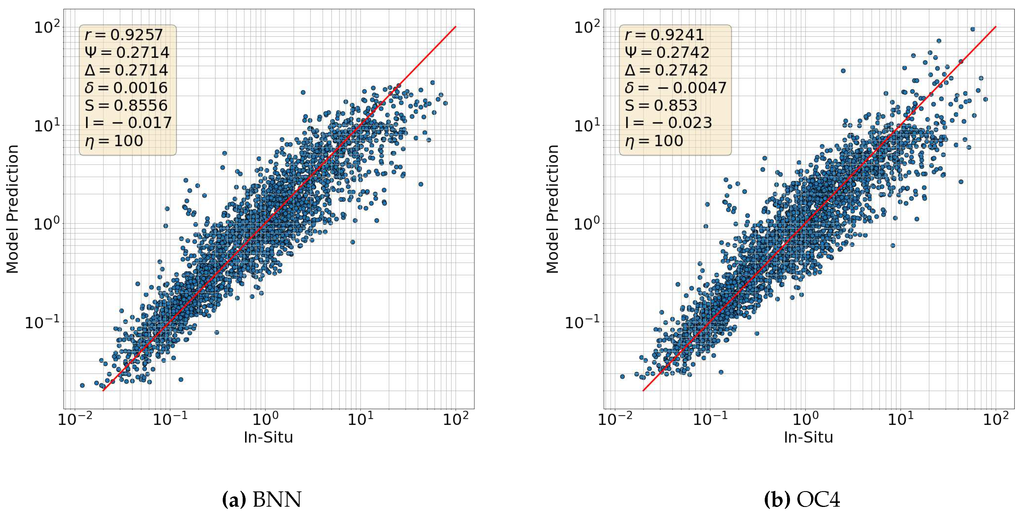
To assess the performance of the models, various statistical measures were computed and are presented in Figure 2. The scatter plots illustrate the relationship between in situ [CHL-a] and their corresponding model predictions for both the BNN MAP and OC4 models. The scatter plots demonstrate a strong correlation between the model predictions and the in situ measurements for both the BNN and OC4 models, with r values of 0.9257 and 0.9241, respectively. Notably, the MAP BNN model performs slightly better than the OC4 model, with higher correlation coefficients and lower errors. Furthermore, the BNN allows for uncertainty estimates through an ensemble of predictions that characterize a posterior distribution for [CHL-a], which implies better characterization of the prediction’s reliability. The slope and intercept of a type II regression are close to 1 and 0 respectively for the BNN’s MAP ( and ) and for OC4 ( and ). Similarly, the errors resulting from the BNN’s MAP ( and ) are slightly smaller than those obtained with OC4 ( and ). In addition, the BNN’s MAP and OC4 predictions show a comparably small bias of and -0.0047, respectively. These results indicate that the BNN’s MAP can predict [CHL-a] with an enhanced accuracy compared to the OC4 algorithm, however, since it is a probabilistic model, the BNN fits the distribution of the data; i.e. the yellow shaded area.
Figure 1.
Scatter plots illustrating the [CHL-a] for the in situ (blue dots), (a) BNN’s MAP prediction (red) and uncertainties represented by (shaded in yellow) for a BNN trained using the SeaWiFS dataset and (b) the OC4 prediction (red) as a function of the MBR.
Figure 1.
Scatter plots illustrating the [CHL-a] for the in situ (blue dots), (a) BNN’s MAP prediction (red) and uncertainties represented by (shaded in yellow) for a BNN trained using the SeaWiFS dataset and (b) the OC4 prediction (red) as a function of the MBR.
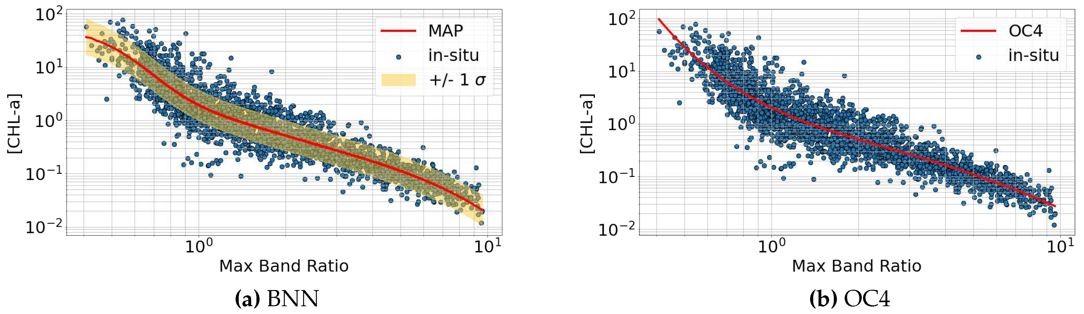
Figure 2.
Scatter plots for the in situ [CHL-a] as a function of the (a) BNN’s MAP and (b) OC4. The scatter plots are accompanied with the resulting error statistics. The plot shows the metrics comparing the MAP and OC4 predictions with the reference measurements. Indicated are the Pearson correlation coefficient (r), root mean squared error (), unbiased root mean squared error (), retreival percentage (), slope (S) and intercept (I) of a type-II regression, and the bias ().
6.2. Comparison with OCI
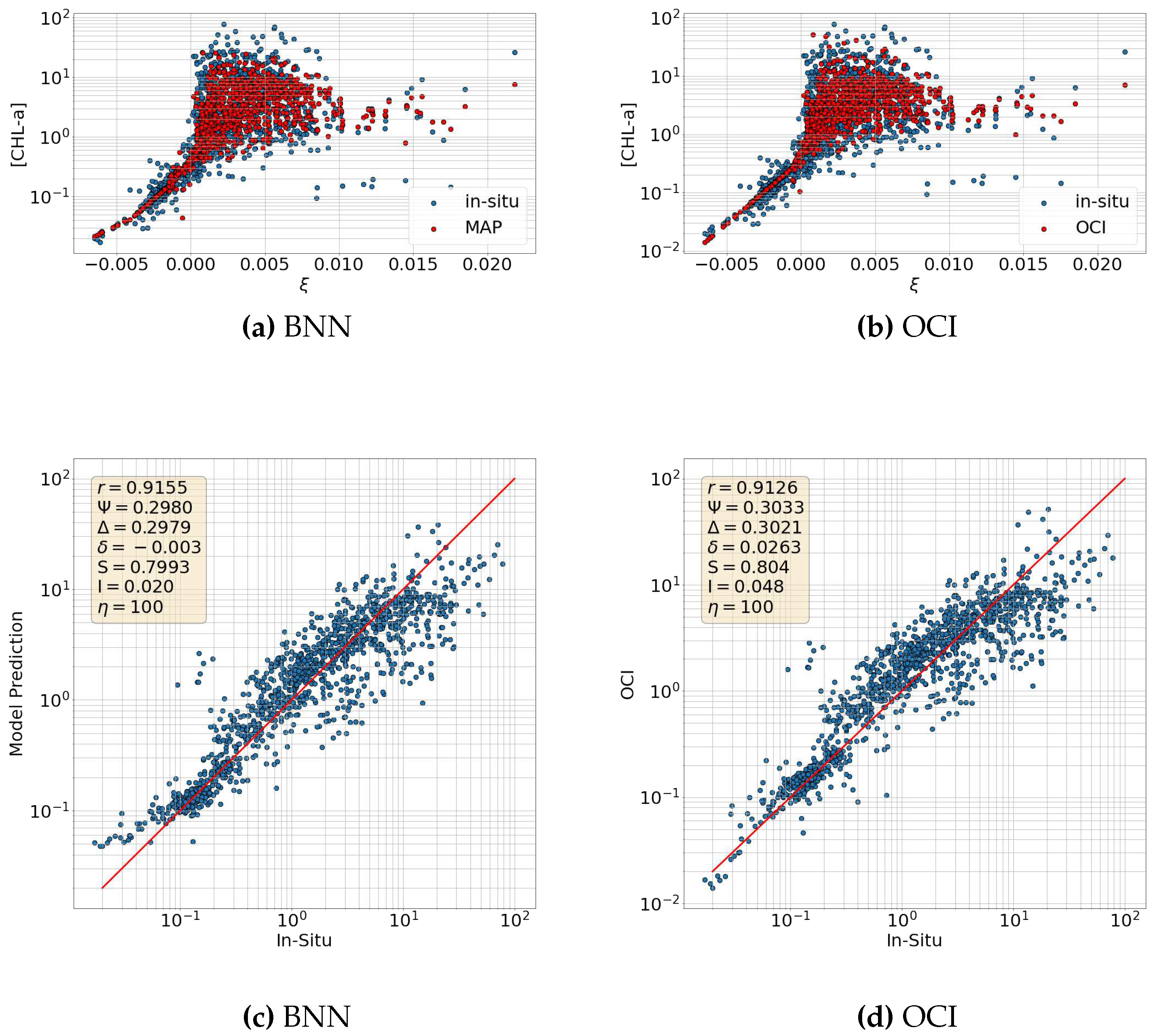
To provide a comprehensive comparison with well-established algorithms, we compare the BNN’s performance to that of the OCI algorithm using the same dataset. The OCI predictions were obtained using the methodology outlined in Section 4, which combines OCI for low [CHL-a] and OC4 for high [CHL-a] with linear interpolation in between. Figure 3a and Figure 3b present scatter plots showing the relationship between [CHL-a] and as predicted by the BNN’s MAP and OCI model, respectively, accompanied by the in situ data. The first plot indicates a general positive agreement between MAP and OCI predictions and in situ data. However, there are some points, primarily representing low [CHL-a] values, that are not captured well by the OCI model.
The scatter plot in Figure 3c and Figure 3d illustrate the relationship between in situ [CHL-a] and their corresponding MAP and OCI predictions, respectively. The figure demonstrates a strong correlation between the MAP predictions and the in situ measurements with a correlation coefficient of , which is slightly higher than the correlation coefficient between the in situ and OCI predictions (). In terms of statistical measures, the OCI model performs slightly less favorably compared to the MAP and OC4 models. Specifically, the OCI model exhibits slightly larger MSEs ( and ) and a larger absolute bias () than the BNN MAP (, and ). Moreover, the type II regression slope and intercept of the MAP (S=0.7993 and I=0.02) are similar to those obtained using the OCI model (S=0.804 and I=0.048). The results further suggest that the BNN MAP offers a smoother change in the predictions when compared to the interpolation adopted by the OCI model. However, the plots also indicate that for [CHL-a] values smaller than , the MAP slightly overestimates [CHL-a] whereas the OCI model appears to have a marginally better agreement with in situ for that range of values.
Figure 3.
(a)-(b) Scatter plots illustrating the [CHL-a] for the in situ (blue dots), (a) BNN’s MAP prediction (red) (b) the OC4 prediction (red) as a function of the MBR and (c)-(d) Scatter plot of the in situ [CHL-a] as a function of the corresponding model predictions for the BNN’s MAP and OCI models, respectively.
6.3. Maximum Band Ratio Bayesian Ocean Model: Generalizability
The in situ match-ups from all satellites demonstrate a strong correlation, as depicted in Figure S.1, illustrating the relationship between in situ [CHL-a] and MBR in the compiled database [40]. To capitalize on this comprehensive database, a BNN model was trained using the combined database comprising of the match-ups retrieved using MODIS, OLCA, OLCB, MERIS, SeaWIFS and VIIRS, benefiting from a larger database than when using match-ups from a single satellite. Note that the MBR values were computed for each satellite independently following their definition in [67] for the OC4 model.
In Figure 4a, a scatter plot showcases the in situ data points alongside an ensemble of 50 sampled ocean colour models. The sampled models exhibit similar behavior with the MBR, with predictions exhibiting a wider spread at extreme MBR values and a tighter spread at the center where the in situ points are densely concentrated. Statistical measures are provided through a scatter plot comparing the in situ points and model predictions in Figure 4b. These measures demonstrate comparable error and correlation values to those obtained from the BNN trained on the SeaWiFS dataset. Particularly, the MAP of the BNN trained on the combined dataset yields a high correlation coefficient , low errors with and , small bias , and reasonably reliable S and I of 0.825 and -0.013, respectively. For comparison, Figure S.2a and S.2b present the OC4 predicted [CHL-a] as a function of the MBR and the corresponding scatter plot of the in situ [CHL-a] against their model-predicted counterparts. The plots indicate that the BNN’s MAP and the OC4 model behave similarly with MBR and achieve comparable statistical measures.
6.4. Reflectances Bayesian Ocean Model
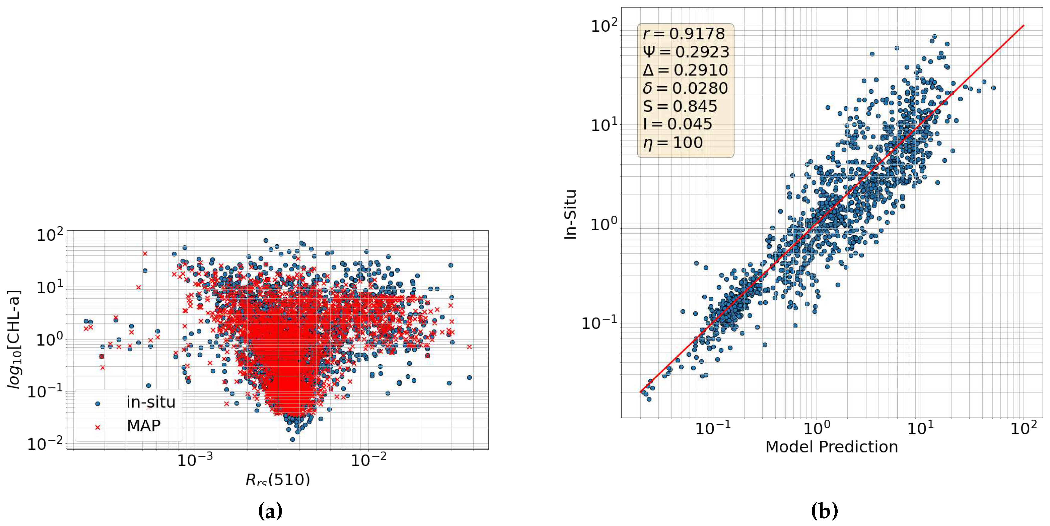
In this experiment, we explore the use of in the blue and green wavelengths, instead of the MBR, as input for the BNN model to construct a higher-dimensional ocean colour model. Specifically, we employ the SeaWiFS at wavelengths of 411 nm, 443 nm, 489 nm, 510 nm, and 555 nm as inputs to the BNN to predict [CHL-a]. The scatter plot depicted in Figure 5a showcases the relationship between the in situ measurements and the MAP predictions of [CHL-a] against the reflectance value at 510 nm ().
The plot in Figure 5b illustrates that the MAP predictions align well with the in situ measurements, displaying consistency throughout the majority of the dataset, with the exception of extreme [CHL-a], which are sparsely represented. Additionally, the plot showcases a strong correlation between the in situ data points and their corresponding model predictions, as evidenced by the high correlation coefficient (r = 0.9178), and the S and I values of 0.845 and 0.045, respectively. Although the resulting errors are relatively small ( and ), they are slightly larger compared to those obtained using the MBR model (Section 6.1).
Figure 5.
(a) Scatter plot of the [CHL-a] against for the in situ measurements and the MAP predictions. (b) Scatter plot illustrating the in situ [CHL-a] measurements against their corresponding MAP predictions.
Figure 5.
(a) Scatter plot of the [CHL-a] against for the in situ measurements and the MAP predictions. (b) Scatter plot illustrating the in situ [CHL-a] measurements against their corresponding MAP predictions.
6.5. Incorporating IOPs
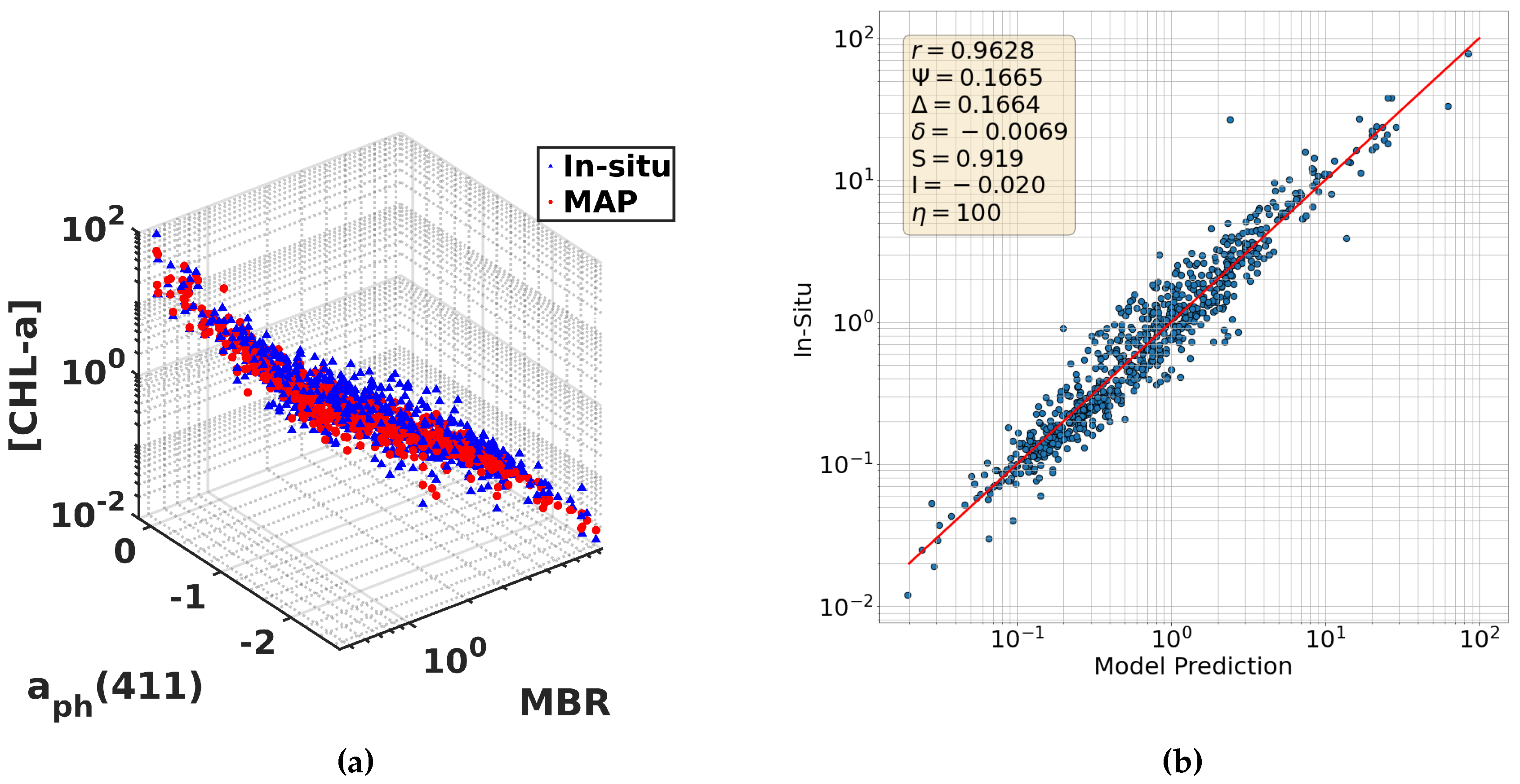
The inclusion of phytoplankton absorption coefficients is also investigated, specifically at wavelengths of 411 nm, 443 nm, 489 nm, 510 nm, and 555 nm, in conjunction with the MBR, as input to the BNN model. IOPs are essential for gaining insights into the characteristics of seawater, providing valuable insights into the composition, [CHL-a], and distribution of optically active substances in the ocean, such as phytoplankton, suspended particles, and colored dissolved organic matter [68]. The results are shown for a BNN model trained using the SeaWiFS dataset under the training conditions described in Section 3.
Figure 6a presents a 3D scatter plot illustrating the relationship between in situ and BNN-predicted [CHL-a] projected along the planes of and MBR. The plot illustrates that the MAP’s [CHL-a] predictions closely follow the behavior of the in situ data. Notably, the inclusion of the absorption coefficient leads to a reduction in prediction uncertainty, as evidenced by the tighter clustering of data points.
Furthermore, Figure 6b showcases a scatter plot comparing the in situ [CHL-a] against the BNN’s MAP predictions. The scatter plot reveals that the model predictions closely align with the in situ data, both qualitatively and quantitatively, exhibiting improved statistical measures in comparison to the previous models. Particularly, a substantial correlation () and slope close to 1 () are observed between the in situ measurements and the model predictions. The figure also illustrates minimal errors, where and , the lowest among all explored models. The MAP also yields a low bias of and intercept , comparable to those obtained with the MBR model in Section 6.1.
Figure 6.
(a) 3D scatter plot illustrating a projection of the [CHL-a] along the MBR and for the in situ measurements and MAP predictions. (b) Scatter plot of the measured in situ [CHL-a] as a function of the MAP predictions with the resulting statistical measures.
Figure 6.
(a) 3D scatter plot illustrating a projection of the [CHL-a] along the MBR and for the in situ measurements and MAP predictions. (b) Scatter plot of the measured in situ [CHL-a] as a function of the MAP predictions with the resulting statistical measures.
6.6. Evaluation of the Probabilistic Ocean Colour Model Using Satellite Observations
The expansive repositories of MODIS and Sentinel-3 imagery allow us to directly compare the predictions of the BNN model with the predictions from traditional OC models. We examine the performance of the BNN in comparison to OC4 for different spatial and temporal resolutions, and ocean colour sensors. By conducting the comparison over a diverse range of regions and environmental conditions, including both hemispheres and distinct coastal and open ocean areas, we can elucidate potential model performance disparities across different marine ecosystems. The areas investigated include the northern and southern Red Sea, the Aegean Sea, and the Baltic Sea, covering a diverse range of oceanographic conditions, as further described later. This comprehensive approach provides a nuanced understanding of the strengths and limitations of the BNN model, facilitating its potential integration into operational oceanographic applications and contributing to advancements in ocean remote sensing and ecological studies. SeaWiFS images were also processed and the resulting BNN predictions are shown in the Supplementary Material.
6.6.1. MODIS
Figure 7 presents a comparison between the MAP predictions of the BNN trained on the merged dataset and the [CHL-a] predictions generated by the OC4 algorithm for a MODIS monthly composite image of the continent of America. The figure provides detailed visualizations for various regions of interest, such as the east and west coasts of the United States, the equatorial region, and the southern hemisphere region in proximity to the coasts of Brazil, Uruguay, and Argentina. Clearly, both the BNN and OC4 models effectively capture the mesoscale features observed in the ocean circulation patterns. The BNN model tends to produce lower [CHL-a] values at extremely high concentrations, a known issue observed in the OC4 algorithm Lavigne et al. 2021. This can be clearly observed, for example, near equatorial regions and along the Gulf Stream. This is better shown in the plot on the right side, which illustrates the difference of the [CHL-a] fields corresponding to the BNN and OC4. The results indicate that the OC4 consistently produces higher [CHL-a] throughout the spatial domain.
Similarly, Figure 8 depicts a side-by-side comparison between the two models and their difference on a scale for the continents of Asia, Europe, Africa, and Australia. The figure also includes zoomed-in plots highlighting regions of interest, such as the Atlantic Ocean near the United Kingdom, the East China Sea, the seas north of Australia, and the waters adjacent to South Africa. Similarly to the results in previous sections, the BNN’s MAP consistently produces lower [CHL-a] in comparison to the predictions made by OC4; e.g. near the United Kingdom. Both predictions clearly illustrate the influence of mesoscale currents on the distribution of [CHL-a]. Overall, the difference is systematically consistent across the domain with the OC4 predicting higher values of [CHL-a].
6.6.2. Sentinel-3
A BNN model was trained using the combined dataset with MBR as input, and used to predict the [CHL-a] for remotely sensed images in the Southern Red Sea, Northern Red Sea, Baltic Sea and Aegean Sea. Furthermore, since the BNN is stochastic, the model is sampled several times to provide an ensemble of predicted [CHL-a] fields, which were used to asses the uncertainty of the BNN prediction.
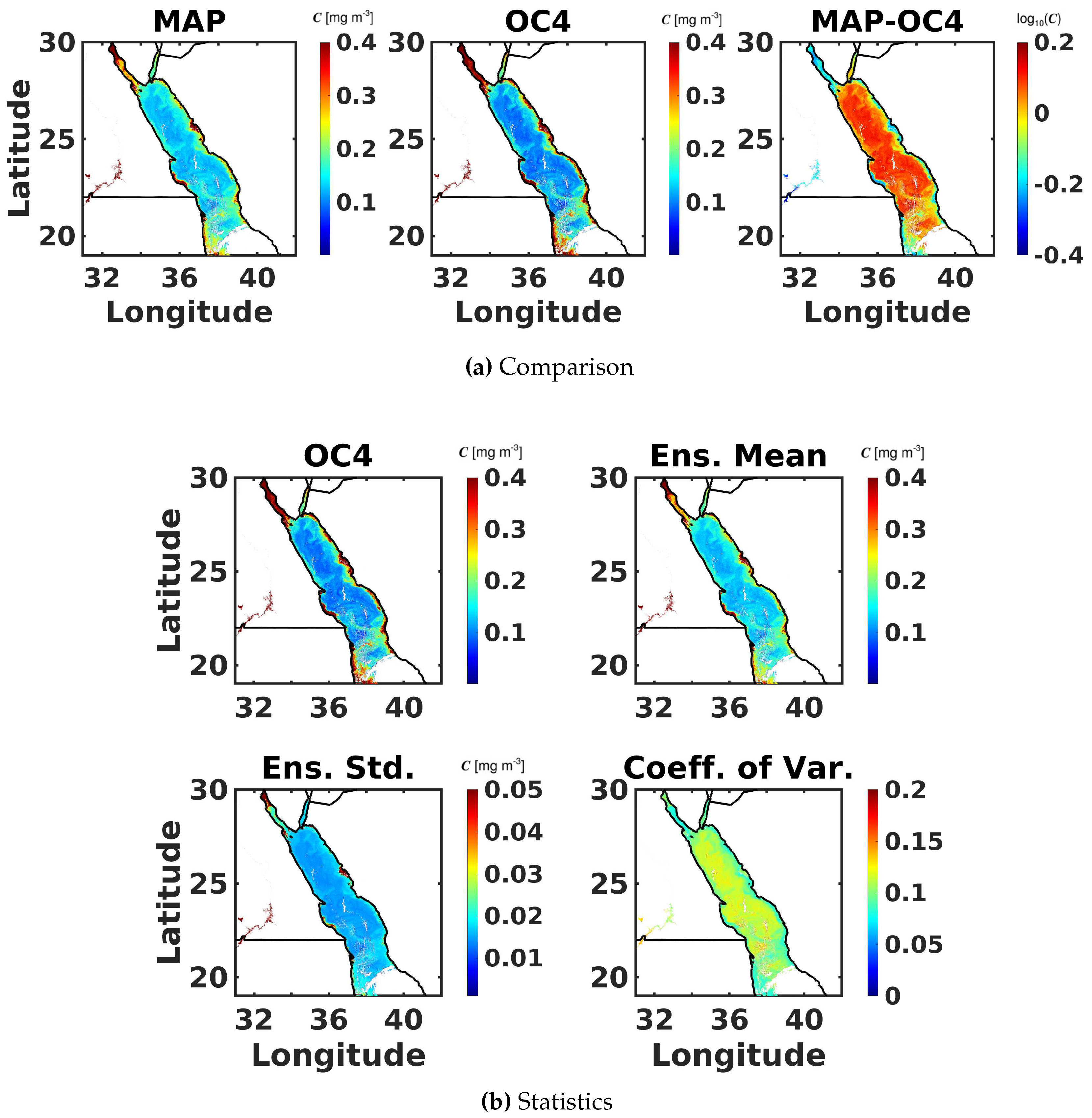
Figure 9a compares the [CHL-a] fields from the BNN’s MAP prediction to that of the OC4 prediction and provides their log difference in the southern part of the Red Sea, a province where satellite-derived observations have acknowledged weaknesses [70,71]. The atmospheric conditions (high evaporation and cloud cover) over the southern Red Sea, especially during summer, make it difficult to obtain consistent and accurate ocean colour data via satellites. It is also the shallowest and most productive part of the of the Red Sea [70], which adds additional layers of complexity in [CHL-a] estimation. Both models seem to predict high [CHL-a] near the eastern and western coasts. Furthermore, both models clearly indicate the mesoscale circulation patterns that impact the transport of nutrients in the southern Red Sea [72]. The MAP predictions appear to capture the lower [CHL-a] values more accurately in the central open waters in comparison to the predicted [CHL-a] by OC4. It is worth noting that the standard OC4 and OCI algorithms have been observed to involve a prediction bias generally overestimating [CHL-a] concentrations in some cases [66,73,74,75]. This is also evident in the difference plot showing a roughly consistent difference between the MAP and OC4 models.
Highlighting the main strength point of the proposed approach, Figure 9b illustrates the OC4 prediction alongside the average, standard deviation and coefficient of variation of an ensemble of 100 BNN predictions. The results indicate that the average of the BNN predictions is close to the OC4 prediction and shows comparable features across the region. Additionally, the BNN allows to quantify uncertainties that are represented here by the standard deviation and coefficient of variation. The standard deviation suggests that the BNN predictions are highly uncertain in the Southern part of the Red Sea near the coastline. On the other hand, the coefficient of variation indicates that these high deviation regions are considerably small relative to the mean [CHL-a] values, and that uncertainties in the open waters are larger in comparison to the mean value in that region. Nevertheless, the coefficient of variation indicates that the standard deviation is within of the mean, which means that the BNN’s prediction captures the associated uncertainties reasonably well for a statistical analysis of the [CHL-a].
Providing further insights to the BNN’s capabilities, Figure 10 illustrates the OC4 prediction alongside a few BNN predicted sample fields. The plots show that the BNN sample predictions capture the same mesoscale transport features, such as eddies, as the ones predicted by OC4. All the BNN predicted samples are correlated with the OC4 prediction, where the high and low [CHL-a] values all lie in the same regions. The shown samples predict lower [CHL-a] values in comparison to those predicted by OC4. Nevertheless, the samples clearly illustrate considerable variability among the predicted samples, which is essential for risk assessment studies that can be conducted in the future in optically challenging areas such as the Baltic Sea.
The optical characteristics of the Baltic Sea are impacted by several key factors, including substantial river discharges, limited interaction with the North Sea, and a relatively shallow sea bed [76]. Another noteworthy factor is the pronounced presence of Colored Dissolved Organic Matter (CDOM), which significantly influences light absorption properties in the region [77]. The Baltic waters also exhibit elevated nutrient levels, increasing primary production, which occasionally leads to very high [CHL-a] [78]. Traditional ocean reflectance-based algorithms, which rely on blue-to-green ratios, are not optimally suited for [CHL-a] retrieval in the Baltic Sea and tend to overestimate its concentrations [78,79]. Figure 11a presents the BNN’s MAP and the corresponding OC4 [CHL-a] predictions and their difference on a scale for the Baltic Sea. The plots indicate comparable [CHL-a] fields between the two model predictions in terms of meso– and fine–scale transport features. The [CHL-a] values, however, are noticeably different between the two model predictions, where the MAP predicts generally lower [CHL-a] values. This could be further observed in the difference plot, which indicates a somewhat systematic difference described by a negative log difference in the whole basin.
Figure 11b illustrates the OC4 prediction, the mean and standard deviation of 100 BNN predictions and the coefficient of variation for the Baltic Sea. Similar to the previous conclusions, the plot indicates that the OC4 prediction overestimates [CHL-a] in comparison to the BNN’s mean prediction. The standard deviation plot suggests that the uncertainties are highest in regions where [CHL-a] are highest. On the other hand, the coefficient of variation plot reveals that the BNN’s prediction has a low coefficient of variation of approximately , meaning that the predictions have low uncertainty. Although the BNN model does not directly correct for high CDOM, incorporating uncertainty during training can reduce the effect of high CDOM on [CHL-a] predictions. The BNN model could, thus, provide a useful tool for early identification of localized HABs in the Baltic Sea.
Figure 12a and Figure 13a illustrate the BNN’s MAP, corresponding OC4 [CHL-a] predictions and their difference for the northern Red Sea and Aegean Sea. The results indicate similar takeaways as those described for the southern Red Sea and Baltic Sea. In particular, the BNN’s MAP [CHL-a] are generally more conservative than those of the OC4 model, where the MAP transitions smoother than OC4 at extreme MBR values, resulting in less intense values. The [CHL-a] values near the northern Red Sea coasts predicted by the BNN’s MAP are lower than those of the OC4. However, the values in the open waters are higher in the BNN predictions for both the Aegean and the northern Red Sea. These results are further evidenced in the difference plot, which indicates that in the open waters of the northern Red Sea, the MAP’s predictions are larger than those of OC4, however, near the coast the OC4 predicts larger [CHL-a] values.
Figure 12b and Figure 13b portray the OC4 [CHL-a] prediction, mean and standard deviation of 100 BNN predictions and their corresponding coefficient of variation. Similarly to previous results, the plots show the BNN’s capability to quantify prediction uncertainties as indicated by the standard deviation, which exhibits a small magnitude for the northern Red Sea and Aegean Sea. The coefficient of variation provides additional information that roughly described a normalized uncertainty estimate of the predictions. The plots indicate that for both basins, the coefficient of variation is approximately , suggesting that the BNN is fairly confident in its predictions for these regions.
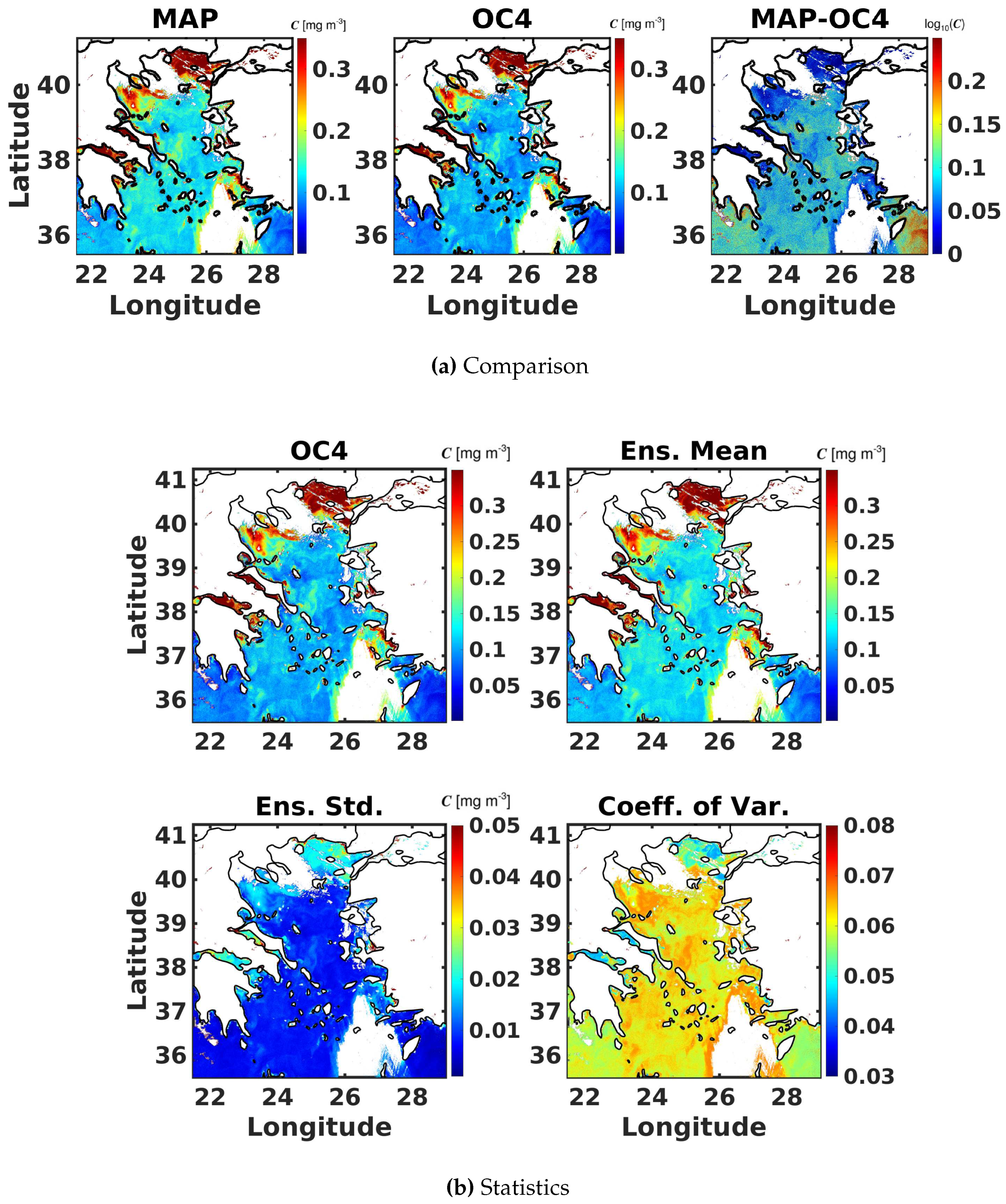
Figure 13.
Daily [CHL-a] image of the Aegean Sea from Sentinel-3 at 300 m spatial resolution: (a) estimated using the MAP and OC4 models alongside their log difference, (b) estimated using OC4, the mean and standard deviation of 100 BNN predicted samples and the corresponding coefficient of variation.
7. Conclusion
This work introduces the use of a bayesian neural network (BNN) for estimating [CHL-a] from remotely sensed data, using the largest available database of in situ match-ups. The BNN’s MAP was shown to outperform established ocean colour models, such as OC4 and OCI, providing reliable estimates for [CHL-a]. Furthermore, the learning-based method allows for more degrees of freedom in ocean colour modeling by involving more input variables, describing the state of the ocean, to predict the chlorophyll-a concentration. The true potential of the BNN model, however, lies in it’s uncertainty quantification capabilities, where the BNN predicts the distribution of potential [CHL-a] values, which builds confidence in the predicted values. Our findings demonstrate that the BNN model exhibits a remarkable capacity to capture mesoscale features and ocean circulation patterns, effectively delineating spatial and temporal variations in [CHL-a] across diverse marine ecosystems. Furthermore, by including uncertainty, the proposed model can provide more accurate information than traditional algorithms for coastal waters when using higher spatial resolution ocean colour imagery such as from the Sentinel-3 OLCI. This can benefit coastal ecosystem health and biodiversity assessments by studying the nutrient circulation, detecting localised HABs, as well as monitoring climate change and other anthropogenic impacts on phytoplankton dynamics.
The BNN’s ability to quantify uncertainty in predictions offers more confidence in the results, particularly in regions with sparse or irregular data coverage, and serves as a crucial step toward fostering informed decision-making in marine research and management. These uncertainty estimates help understand when and where the BNN predictions are reliable, as opposed to other regions where uncertainties are large and additional data may be necessary to improve prediction accuracy. The southern Red Sea (Figure 9) is an example of a region, where regional tuning of the ocean colour model is needed in order to increase the accuracy of [CHL-a] estimation. Other such shallow coastal environments can be identified globally by applying the BNN model. By tuning the model further with more high quality regional observations, new information regarding their phytoplankton phenology may emerge.
The introduction of BNN models also creates new possibilities in the field of ocean colour remote sensing. Future research can expand the scope of this work by incorporating additional variables such as sea surface temperature to further improve the accuracy of [CHL-a] estimates, and estimating [CHL-a] along the water column.
Supplementary Materials
The following supporting information can be downloaded at the website of this paper posted on Preprints.org
Author Contributions
Conceptualization, M.H. and N.P.; methodology, M.H. and N.P.; software, M.H.; validation, M.H., N.P., R.B., D.R. and I.H.; formal analysis, M.H, N.P, R.B., D.R., O.K. and I.H; investigation, M.H, N.P, R.B., D.R., O.K. and I.H; resources, O.K. and I.H; data curation, M.H and N.P; writing—original draft preparation, M.H and N.P; writing—review and editing, M.H, N.P, R.B., D.R., O.K. and I.H; visualization, M.H; supervision, R.B., D.R., O.K. and I.H; project administration, R.B., D.R., O.K. and I.H; funding acquisition, R.B., O.K. and I.H All authors have read and agreed to the published version of the manuscript.
Funding
Research reported in this publication was supported by the Virtual Red Sea Initiative Award #REP/1/3268-01-01. RJW Brewin is supported by a UKRI Future Leader Fellowship (MR/V022792/1).
Institutional Review Board Statement
Not applicable.
Informed Consent Statement
Not applicable.
Data Availability Statement
All the data used for this study are openly accessible through https://doi.pangaea.de/10.1594/PANGAEA.941318.
Conflicts of Interest
The authors declare no conflicts of interest.
Appendix A Stochastic Variational Inference
Appendix A.1. Bayesian Statistics
In efforts to introduce stochastic variational inference (SVI), we begin by introducing the notation and the foundational statistics. In a probabilistic models, the response is related to the input random variables through the joint probability distribution. A model with observations , latent random variables and parameterized with can assume the joint density function given by:
where, is the prior distribution of and denotes the likelihood.
Generally, probabilistic modeling could be made efficient by decomposing the joint probability distribution into simpler conditional probability functions , such that can be efficiently sampled, is differentiable with respect to and pointwise probability densities could be efficiently computed.
Inference can be done following Bayes rule by evaluating the posterior distribution over :
where the denominator is called the marginal likelihood or evidence. Finally, it is generally preferable to learn the parameters that maximize the marginal likelihood, where:
Furthermore, predictions for new input data are performed with the posterior predictive distribution according to:
where predictions from the posterior predictive distribution corresponding to are called maximum a posteriori probability (MAP) estimates.
Appendix A.2. Variational Inference
In the previous section, computations require evaluating complex integrals that are computationally non–trivial requiring approximation algorithms, namely variational inference. SVI is based on variational inference, which involves approximating the posterior distribution with a simpler distribution from a predefined family. This family of distributions is typically chosen to be tractable, such as a mean-field Gaussian or a neural network.
Variational inference algorithms aim at finding by computing the so-called variational distribution over the latent variables of the model , which is an approximation of the true unknown posterior . Essentially, the objective is to find an approximate joint probability function that is valid over the space of latent random variables in the model, and this is done by formulating the inference problem as an optimization problem as opposed to a sampling one. The probabilistic model, Bayesian neural network in this case, is first defined, where the model has to be differentiable and computationally–efficient to evaluate. In the probabilistic framework, the parameters of the model are treated as random variables and are each assigned a prior distribution. Furthermore, a likelihood distribution is also assigned to the model output, which is typically application–specific.
In variational inference, the parameters of the model are learned by solving an optimization problem that moves the variational posterior distribution closer to the true posterior distribution. In general, the evidence lower bound (ELBO) loss is used to update the parameters of the probabilistic model, such that the approximate posterior distribution is closer to the true posterior. The ELBO loss is defined as the difference between the expected log-likelihood of the data under the approximating distribution and the KL divergence between the approximating distribution and the prior distribution over the latent variables. Maximizing the ELBO loss is shown to be equivalent to minimizing the Kullback–Leibler (KL) divergence between the approximate and true posterior distributions, which helps find the best possible approximation to the true posterior within the chosen family of distributions. In stochastic variational inference, stochastic optimization techniques are typically adopted to efficiently handle large datasets. In particular, SVI randomly selects a subset (or minibatch) of the data to estimate the gradient of the objective function instead of processing entire datasets in each iteration, which improves the scalability of such methods.
Once training is terminated and a suitably trained model is obtained, the variational posterior is sampled. Since the true posterior is intractable, the posterior predictive estimates are obtained according to:
In practice, the posterior predictive could then be sampled by first drawing a random sample from the approximate posterior and used to sample .
References
- Harris, G. Phytoplankton ecology: structure, function and fluctuation; Springer Science & Business Media, 2012.
- Jones, R.I. Phytoplankton, primary production and nutrient cycling. Aquatic humic substances: ecology and biogeochemistry 1998, pp. 145–175. [CrossRef]
- Falkowski, P.G.; Raven, J.A. Aquatic photosynthesis; Princeton University Press, 2013.
- Hays, G.C.; Richardson, A.J.; Robinson, C. Climate change and marine plankton. Trends in ecology & evolution 2005, 20, 337–344. [CrossRef]
- Haeder, D.P.; Villafane, V.E.; Helbling, E.W. Productivity of aquatic primary producers under global climate change. Photochemical & Photobiological Sciences 2014, 13, 1370–1392. [CrossRef]
- Basu, S.; Mackey, K.R. Phytoplankton as key mediators of the biological carbon pump: Their responses to a changing climate. Sustainability 2018, 10, 869. [CrossRef]
- Falkowski, P.G. The role of phytoplankton photosynthesis in global biogeochemical cycles. Photosynthesis research 1994, 39, 235–258. [CrossRef]
- Platt, T.; Fuentes-Yaco, C.; Frank, K.T. Spring algal bloom and larval fish survival. Nature 2003, 423, 398–399. [CrossRef]
- Anderson, D.M.; Glibert, P.M.; Burkholder, J.M. Harmful algal blooms and eutrophication: nutrient sources, composition, and consequences. Estuaries 2002, 25, 704–726. [CrossRef]
- Klemas, V. Remote sensing of algal blooms: an overview with case studies. Journal of coastal research 2012, 28, 34–43. [CrossRef]
- Racault, M.F.; Platt, T.; Sathyendranath, S.; Ağirbaş, E.; Martinez Vicente, V.; Brewin, R. Plankton indicators and ocean observing systems: support to the marine ecosystem state assessment. Journal of Plankton Research 2014, 36, 621–629. [CrossRef]
- Platt, T.; White III, G.N.; Zhai, L.; Sathyendranath, S.; Roy, S. The phenology of phytoplankton blooms: Ecosystem indicators from remote sensing. Ecological Modelling 2009, 220, 3057–3069. [CrossRef]
- Hazen, E.L.; Suryan, R.M.; Santora, J.A.; Bograd, S.J.; Watanuki, Y.; Wilson, R.P. Scales and mechanisms of marine hotspot formation. Marine Ecology Progress Series 2013, 487, 177–183. [CrossRef]
- Racault, M.F.; Le Quéré, C.; Buitenhuis, E.; Sathyendranath, S.; Platt, T. Phytoplankton phenology in the global ocean. Ecological Indicators 2012, 14, 152–163. [CrossRef]
- Gokul, E.A.; Raitsos, D.E.; Gittings, J.A.; Alkawri, A.; Hoteit, I. Remotely sensing harmful algal blooms in the Red Sea. PLoS One 2019, 14, e0215463. [CrossRef]
- Lin, J.; Miller, P.I.; Jönsson, B.F.; Bedington, M. Early Warning of Harmful Algal Bloom Risk Using Satellite Ocean Color and Lagrangian Particle Trajectories. Frontiers in Marine Science 2021, 8. [CrossRef]
- Shu, C.; Xiu, P.; Xing, X.; Qiu, G.; Ma, W.; Brewin, R.J.; Ciavatta, S. Biogeochemical Model Optimization by Using Satellite-Derived Phytoplankton Functional Type Data and BGC-Argo Observations in the Northern South China Sea. Remote Sensing 2022, 14, 1297. [CrossRef]
- Joint, I.; Groom, S.B. Estimation of phytoplankton production from space: current status and future potential of satellite remote sensing. Journal of experimental marine Biology and Ecology 2000, 250, 233–255. [CrossRef]
- Morel, A.; Prieur, L. Analysis of variations in ocean color1. Limnology and Oceanography 1977, 22, 709–722, [https://aslopubs.onlinelibrary.wiley.com/doi/pdf/10.4319/lo.1977.22.4.0709]. [CrossRef]
- Bricaud, A.; Babin, M.; Morel, A.; Claustre, H. Variability in the chlorophyll-specific absorption coefficients of natural phytoplankton: Analysis and parameterization. Journal of Geophysical Research: Oceans 1995, 100, 13321–13332. [CrossRef]
- Groom, S.; Sathyendranath, S.; Ban, Y.; Bernard, S.; Brewin, R.; Brotas, V.; Brockmann, C.; Chauhan, P.; Choi, J.k.; Chuprin, A.; others. Satellite ocean colour: current status and future perspective. Frontiers in Marine Science 2019, 6, 485. [CrossRef]
- O’Reilly, J.E.; Werdell, P.J. Chlorophyll algorithms for ocean color sensors-OC4, OC5 & OC6. Remote sensing of environment 2019, 229, 32–47. [CrossRef]
- Mélin, F.; others. Uncertainties in ocean colour remote sensing 2019.
- Neil, C.; Spyrakos, E.; Hunter, P.D.; Tyler, A.N. A global approach for chlorophyll-a retrieval across optically complex inland waters based on optical water types. Remote Sensing of Environment 2019, 229, 159–178. [CrossRef]
- Doerffer, R.; Schiller, H. The MERIS Case 2 water algorithm. International Journal of Remote Sensing 2007, 28, 517–535. [CrossRef]
- Yu, B.; Xu, L.; Peng, J.; Hu, Z.; Wong, A. Global chlorophyll-a concentration estimation from moderate resolution imaging spectroradiometer using convolutional neural networks. Journal of Applied Remote Sensing 2020, 14, 034520–034520. [CrossRef]
- Ye, H.; Tang, S.; Yang, C. Deep learning for Chlorophyll-a concentration retrieval: A case study for the Pearl River Estuary. Remote Sensing 2021, 13, 3717. [CrossRef]
- Fan, D.; He, H.; Wang, R.; Zeng, Y.; Fu, B.; Xiong, Y.; Liu, L.; Xu, Y.; Gao, E. CHLNET: A novel hybrid 1D CNN-SVR algorithm for estimating ocean surface chlorophyll-a. Frontiers in Marine Science 2022, 9, 934536. [CrossRef]
- Hadjal, M.; Medina-Lopez, E.; Ren, J.; Gallego, A.; McKee, D. An artificial neural network algorithm to retrieve chlorophyll a for Northwest European shelf seas from top of atmosphere ocean colour reflectance. Remote sensing 2022, 14, 3353. [CrossRef]
- MacKay, D.J. Bayesian neural networks and density networks. Nuclear Instruments and Methods in Physics Research Section A: Accelerators, Spectrometers, Detectors and Associated Equipment 1995, 354, 73–80. Proceedings of the Third Workshop on Neutron Scattering Data Analysis. [CrossRef]
- Jospin, L.V.; Laga, H.; Boussaid, F.; Buntine, W.; Bennamoun, M. Hands-On Bayesian Neural Networks—A Tutorial for Deep Learning Users. IEEE Computational Intelligence Magazine 2022, 17, 29–48. [CrossRef]
- Shen, G.; Chen, X.; Deng, Z. Variational Learning of Bayesian Neural Networks via Bayesian Dark Knowledge. Proceedings of the Twenty-Ninth International Joint Conference on Artificial Intelligence, IJCAI-20; Bessiere, C., Ed. International Joint Conferences on Artificial Intelligence Organization, 2020, pp. 2037–2043. Main track, . [CrossRef]
- Izmailov, P.; Vikram, S.; Hoffman, M.D.; Wilson, A.G.G. What Are Bayesian Neural Network Posteriors Really Like? Proceedings of the 38th International Conference on Machine Learning; Meila, M.; Zhang, T., Eds. PMLR, 2021, Vol. 139, Proceedings of Machine Learning Research, pp. 4629–4640.
- Magris, M.; Iosifidis, A. Bayesian learning for neural networks: an algorithmic survey. Artificial Intelligence Review 2023, 56, 11773–11823. [CrossRef]
- Kendall, A.; Gal, Y. What Uncertainties Do We Need in Bayesian Deep Learning for Computer Vision? Advances in Neural Information Processing Systems; Guyon, I.; Luxburg, U.V.; Bengio, S.; Wallach, H.; Fergus, R.; Vishwanathan, S.; Garnett, R., Eds. Curran Associates, Inc., 2017, Vol. 30.
- Goan, E.; Fookes, C. Bayesian Neural Networks: An Introduction and Survey. In Case Studies in Applied Bayesian Data Science: CIRM Jean-Morlet Chair, Fall 2018; Mengersen, K.L.; Pudlo, P.; Robert, C.P., Eds.; Springer International Publishing: Cham, 2020; pp. 45–87. [CrossRef]
- Chen, B.; Zhang, A.; Cao, L. Autonomous intelligent decision-making system based on Bayesian SOM neural network for robot soccer. Neurocomputing 2014, 128, 447–458. [CrossRef]
- Abdullah, A.A.; Hassan, M.M.; Mustafa, Y.T. A Review on Bayesian Deep Learning in Healthcare: Applications and Challenges. IEEE Access 2022, 10, 36538–36562. [CrossRef]
- Werther, M.; Odermatt, D.; Simis, S.G.; Gurlin, D.; Lehmann, M.K.; Kutser, T.; Gupana, R.; Varley, A.; Hunter, P.D.; Tyler, A.N.; Spyrakos, E. A Bayesian approach for remote sensing of chlorophyll-a and associated retrieval uncertainty in oligotrophic and mesotrophic lakes. Remote Sensing of Environment 2022, 283, 113295. [CrossRef]
- Valente, A.; Sathyendranath, S.; Brotas, V.; Groom, S.; Grant, M.; Jackson, T.; Chuprin, A.; Taberner, M.; Airs, R.; Antoine, D.; Arnone, R.; Balch, W.M.; Barker, K.; Barlow, R.; Bélanger, S.; Berthon, J.F.; Beşiktepe, c.; Borsheim, Y.; Bracher, A.; Brando, V.; Brewin, R.J.W.; Canuti, E.; Chavez, F.P.; Cianca, A.; Claustre, H.; Clementson, L.; Crout, R.; Ferreira, A.; Freeman, S.; Frouin, R.; García-Soto, C.; Gibb, S.W.; Goericke, R.; Gould, R.; Guillocheau, N.; Hooker, S.B.; Hu, C.; Kahru, M.; Kampel, M.; Klein, H.; Kratzer, S.; Kudela, R.; Ledesma, J.; Lohrenz, S.; Loisel, H.; Mannino, A.; Martinez-Vicente, V.; Matrai, P.; McKee, D.; Mitchell, B.G.; Moisan, T.; Montes, E.; Muller-Karger, F.; Neeley, A.; Novak, M.; O’Dowd, L.; Ondrusek, M.; Platt, T.; Poulton, A.J.; Repecaud, M.; Röttgers, R.; Schroeder, T.; Smyth, T.; Smythe-Wright, D.; Sosik, H.M.; Thomas, C.; Thomas, R.; Tilstone, G.; Tracana, A.; Twardowski, M.; Vellucci, V.; Voss, K.; Werdell, J.; Wernand, M.; Wojtasiewicz, B.; Wright, S.; Zibordi, G. A compilation of global bio-optical in situ data for ocean colour satellite applications – version three. Earth System Science Data 2022, 14, 5737–5770. [CrossRef]
- Werdell, P.; Bailey, S. The SeaWiFS Bio-optical Archive and Storage System (SeaBASS): Current Architecture and Implementation. technical memorandum 2002-211617, NASA Goddard Space Flight Center, Greenbelt, Maryland, 2002.
- Werdell, P.J.; Bailey, S.W. An improved in-situ bio-optical data set for ocean color algorithm development and satellite data product validation. Remote Sensing of Environment 2005, 98, 122–140. [CrossRef]
- Barker, K.; Mazeran, C.; Lerebourg, C.; Bouvet, M.; Antoine, D.; Ondrusek, M.; Zibordi, G.; Lavender, S. Mermaid: The MERIS matchup in-situ database. Proceedings of the 2nd (A) ATSR and MERIS Workshop, Frascati, Italy, 2008, pp. 22–26.
- Matrai, P.; Olson, E.; Suttles, S.; Hill, V.; Codispoti, L.; Light, B.; Steele, M. Synthesis of primary production in the Arctic Ocean: I. Surface waters, 1954–2007. Progress in Oceanography 2013, 110, 93–106. [CrossRef]
- Devine, L.; Galbraith, P.S.; Joly, P.; Plourde, S.; Saint-Amand.; Pierre, J.S.; Starr, M. Chemical and biological oceanographic conditions in the estuary and Gulf of St. Lawrence during 2015; Fisheries and Oceans Canada, Ecosystems and Oceans Science, 2015.
- Nechad, B.; Ruddick, K.; Schroeder, T.; Oubelkheir, K.; Blondeau-Patissier, D.; Cherukuru, N.; Brando, V.; Dekker, A.; Clementson, L.; Banks, A.C.; Maritorena, S.; Werdell, P.J.; Sá, C.; Brotas, V.; Caballero de Frutos, I.; Ahn, Y.H.; Salama, S.; Tilstone, G.; Martinez-Vicente, V.; Foley, D.; McKibben, M.; Nahorniak, J.; Peterson, T.; Siliò-Calzada, A.; Röttgers, R.; Lee, Z.; Peters, M.; Brockmann, C. CoastColour Round Robin data sets: a database to evaluate the performance of algorithms for the retrieval of water quality parameters in coastal waters. Earth System Science Data 2015, 7, 319–348. [CrossRef]
- Peloquin, J.M.; Swan, C.; Gruber, N.; Vogt, M.; Claustre, H.; Ras, J.; Uitz, J.; Barlow, R.G.; Behrenfeld, M.J.; Bidigare, R.R.; Dierssen, H.M.; Ditullio, G.; Fernández, E.; Gallienne, C.; Gibb, S.W.; Goericke, R.; Harding, L.; Head, E.J.H.; Holligan, P.M.; Hooker, S.B.; Karl, D.; Landry, M.R.; Letelier, R.; Llewellyn, C.; Lomas, M.W.; Lucas, M.; Mannino, A.; Marty, J.C.; Mitchell, B.G.; Muller-Karger, F.E.; Nelson, N.; O’Brien, C.J.; Prezelin, B.; Repeta, D.J.; Smith, W.O.J.; Smythe-Wright, D.; Stumpf, R.; Subramaniam, A.; Suzuki, K.; Trees, C.; Vernet, M.; Wasmund, N.; Wright, S. The MAREDAT global database of high performance liquid chromatography marine pigment measurements - Gridded data product (NetCDF) - Contribution to the MAREDAT World Ocean Atlas of Plankton Functional Types, 2013. [CrossRef]
- Clark, D.; Murphy, M.; Yarbrough, M.; Feinholz, M.; Flora, S.; Broenkow, W.; Johnson, B.; Brown, S.; Kim, Y.; Mueller, J. MOBY, A Radiometric Buoy for Performance Monitoring and Vicarious Calibration of Satellite Ocean Color Sensors: Measurement and Data Analysis Protocols, 2003.
- Neal, R.M. Bayesian Learning for Neural Networks; Springer New York, 1996. [CrossRef]
- Samaniego, F.J. A comparison of the Bayesian and frequentist approaches to estimation; Vol. 24, Springer, 2010.
- Chen, T.; Chen, H. Universal approximation to nonlinear operators by neural networks with arbitrary activation functions and its application to dynamical systems. IEEE Transactions on Neural Networks 1995, 6, 911–917. [CrossRef]
- Moore, T.S.; Campbell, J.W.; Dowell, M.D. A class-based approach to characterizing and mapping the uncertainty of the MODIS ocean chlorophyll product. Remote Sensing of Environment 2009, 113, 2424–2430. [CrossRef]
- IOCCG. Uncertainties in Ocean Colour Remote Sensing. International Ocean Colour Coordinating Group, Dartmouth, Canada 2019. [CrossRef]
- Amini, A.; Schwarting, W.; Soleimany, A.; Rus, D. Deep evidential regression. Advances in Neural Information Processing Systems 2020, 33, 14927–14937.
- Bingham, E.; Chen, J.P.; Jankowiak, M.; Obermeyer, F.; Pradhan, N.; Karaletsos, T.; Singh, R.; Szerlip, P.; Horsfall, P.; Goodman, N.D. Pyro: Deep Universal Probabilistic Programming. J. Mach. Learn. Res. 2019, 20, 973–978. [CrossRef]
- Hoffman, M.D.; Blei, D.M.; Wang, C.; Paisley, J. Stochastic variational inference. Journal of Machine Learning Research 2013.
- Ranganath, R.; Gerrish, S.; Blei, D. Black box variational inference. Artificial intelligence and statistics. PMLR, 2014, pp. 814–822.
- Blei, D.M.; Kucukelbir, A.; McAuliffe, J.D. Variational Inference: A Review for Statisticians. Journal of the American Statistical Association 2017, 112, 859–877, [https://doi.org/10.1080/01621459.2017.1285773]. [CrossRef]
- Kingma, D.P.; Welling, M. Auto-Encoding Variational Bayes, 2022, [arXiv:stat.ML/1312.6114].
- Olivier, A.; Shields, M.D.; Graham-Brady, L. Bayesian neural networks for uncertainty quantification in data-driven materials modeling. Computer Methods in Applied Mechanics and Engineering 2021, 386, 114079. [CrossRef]
- Kingma, D.P.; Ba, J. Adam: A Method for Stochastic Optimization, 2017, [arXiv:cs.LG/1412.6980].
- O’Reilly, J.; Maritorena, S.; Siegel, D.; O’Brien, M.; Toole, D.; Mitchell, B.; Kahru, M.; Chavez, F.; Strutton, P.; Cota, G. Ocean color chlorophyll a algorithms for SeaWiFS, OC2, and OC4: Technical report. SeaWiFS postlaunch technical report series, SeaWiFS postlaunch calibration and validation analyses part 3,Vol. 11, NASA, Goddard Space Flight Center, Greenbelt, Maryland, 2000.
- Hammoud, M.A.E.R.; Mittal, H.V.R.; Le Maître, O.; Hoteit, I.; Knio, O. Variance-based sensitivity analysis of oil spill predictions in the Red Sea region. Frontiers in Marine Science 2023, 10. [CrossRef]
- Hu, C.; Lee, Z.; Franz, B. Chlorophyll aalgorithms for oligotrophic oceans: A novel approach based on three-band reflectance difference. Journal of Geophysical Research: Oceans 2012, 117, [https://agupubs.onlinelibrary.wiley.com/doi/pdf/10.1029/2011JC007395]. [CrossRef]
- Hu, C.; Lee, Z.; Franz, B. Chlorophyll aalgorithms for oligotrophic oceans: A novel approach based on three-band reflectance difference. Journal of Geophysical Research: Oceans 2012, 117, [https://agupubs.onlinelibrary.wiley.com/doi/pdf/10.1029/2011JC007395]. [CrossRef]
- Brewin, R.J.; Sathyendranath, S.; Müller, D.; Brockmann, C.; Deschamps, P.Y.; Devred, E.; Doerffer, R.; Fomferra, N.; Franz, B.; Grant, M.; Groom, S.; Horseman, A.; Hu, C.; Krasemann, H.; Lee, Z.; Maritorena, S.; Mélin, F.; Peters, M.; Platt, T.; Regner, P.; Smyth, T.; Steinmetz, F.; Swinton, J.; Werdell, J.; White, G.N. The Ocean Colour Climate Change Initiative: III. A round-robin comparison on in-water bio-optical algorithms. Remote Sensing of Environment 2015, 162, 271–294. [CrossRef]
- O’Reilly, J.E.; Werdell, P.J. Chlorophyll algorithms for ocean color sensors - OC4, OC5 & OC6. Remote Sensing of Environment 2019, 229, 32–47. [CrossRef]
- Woźniak, S.B.; Meler, J.; Stoń-Egiert, J. Inherent optical properties of suspended particulate matter in the southern Baltic Sea in relation to the concentration, composition and characteristics of the particle size distribution; new forms of multicomponent parameterizations of optical properties. Journal of Marine Systems 2022, 229, 103720. [CrossRef]
- Lavigne, H.; Van der Zande, D.; Ruddick, K.; Cardoso Dos Santos, J.; Gohin, F.; Brotas, V.; Kratzer, S. Quality-control tests for OC4, OC5 and NIR-red satellite chlorophyll-a algorithms applied to coastal waters. Remote Sensing of Environment 2021, 255, 112237. [CrossRef]
- Raitsos, D.E.; Pradhan, Y.; Brewin, R.J.W.; Stenchikov, G.; Hoteit, I. Remote Sensing the Phytoplankton Seasonal Succession of the Red Sea. PLOS ONE 2013, 8, 1–9. [CrossRef]
- Raitsos, D.E.; Yi, X.; Platt, T.; Racault, M.F.; Brewin, R.J.W.; Pradhan, Y.; Papadopoulos, V.P.; Sathyendranath, S.; Hoteit, I. Monsoon oscillations regulate fertility of the Red Sea. Geophysical Research Letters 2015, 42, 855–862, [https://agupubs.onlinelibrary.wiley.com/doi/pdf/10.1002/2014GL062882]. [CrossRef]
- Raitsos, D.E.; Brewin, R.J.W.; Zhan, P.; Dreano, D.; Pradhan, Y.; Nanninga, G.B.; Hoteit, I. Sensing coral reef connectivity pathways from space. Scientific Reports 2017, 7, 9338. [CrossRef]
- Garcia, V.M.T.; Signorini, S.; Garcia, C.A.E.; McClain, C.R. Empirical and semi-analytical chlorophyll algorithms in the south-western Atlantic coastal region (25–40°S and 60–45°W). International Journal of Remote Sensing 2006, 27, 1539–1562, [https://doi.org/10.1080/01431160500382857]. [CrossRef]
- Brewin, R.J.; Raitsos, D.E.; Pradhan, Y.; Hoteit, I. Comparison of chlorophyll in the Red Sea derived from MODIS-Aqua and in vivo fluorescence. Remote Sensing of Environment 2013, 136, 218–224.
- Racault, M.F.; Raitsos, D.E.; Berumen, M.L.; Brewin, R.J.; Platt, T.; Sathyendranath, S.; Hoteit, I. Phytoplankton phenology indices in coral reef ecosystems: Application to ocean-color observations in the Red Sea. Remote Sensing of Environment 2015, 160, 222–234. [CrossRef]
- Darecki, M.; Stramski, D. An evaluation of MODIS and SeaWiFS bio-optical algorithms in the Baltic Sea. Remote sensing of Environment 2004, 89, 326–350.
- Kowalczuk, P. Seasonal variability of yellow substance absorption in the surface layer of the Baltic Sea. Journal of Geophysical Research: Oceans 1999, 104, 30047–30058.
- Pitarch, J.; Volpe, G.; Colella, S.; Krasemann, H.; Santoleri, R. Remote sensing of chlorophyll in the Baltic Sea at basin scale from 1997 to 2012 using merged multi-sensor data. Ocean Science 2016, 12, 379–389.
- Darecki, M.; Weeks, A.; Sagan, S.; Kowalczuk, P.; Kaczmarek, S. Optical characteristics of two contrasting Case 2 waters and their influence on remote sensing algorithms. Continental Shelf Research 2003, 23, 237–250.
Figure 4.
(a) Plot illustrating [CHL-a] curves as a function of MBR for 50 randomly sampled BNN models (colored curves) and the in situ data points. (b) Scatter plot showing the in situ [CHL-a] measurements against the MAP predictions for a BNN trained using the combined dataset.
Figure 4.
(a) Plot illustrating [CHL-a] curves as a function of MBR for 50 randomly sampled BNN models (colored curves) and the in situ data points. (b) Scatter plot showing the in situ [CHL-a] measurements against the MAP predictions for a BNN trained using the combined dataset.
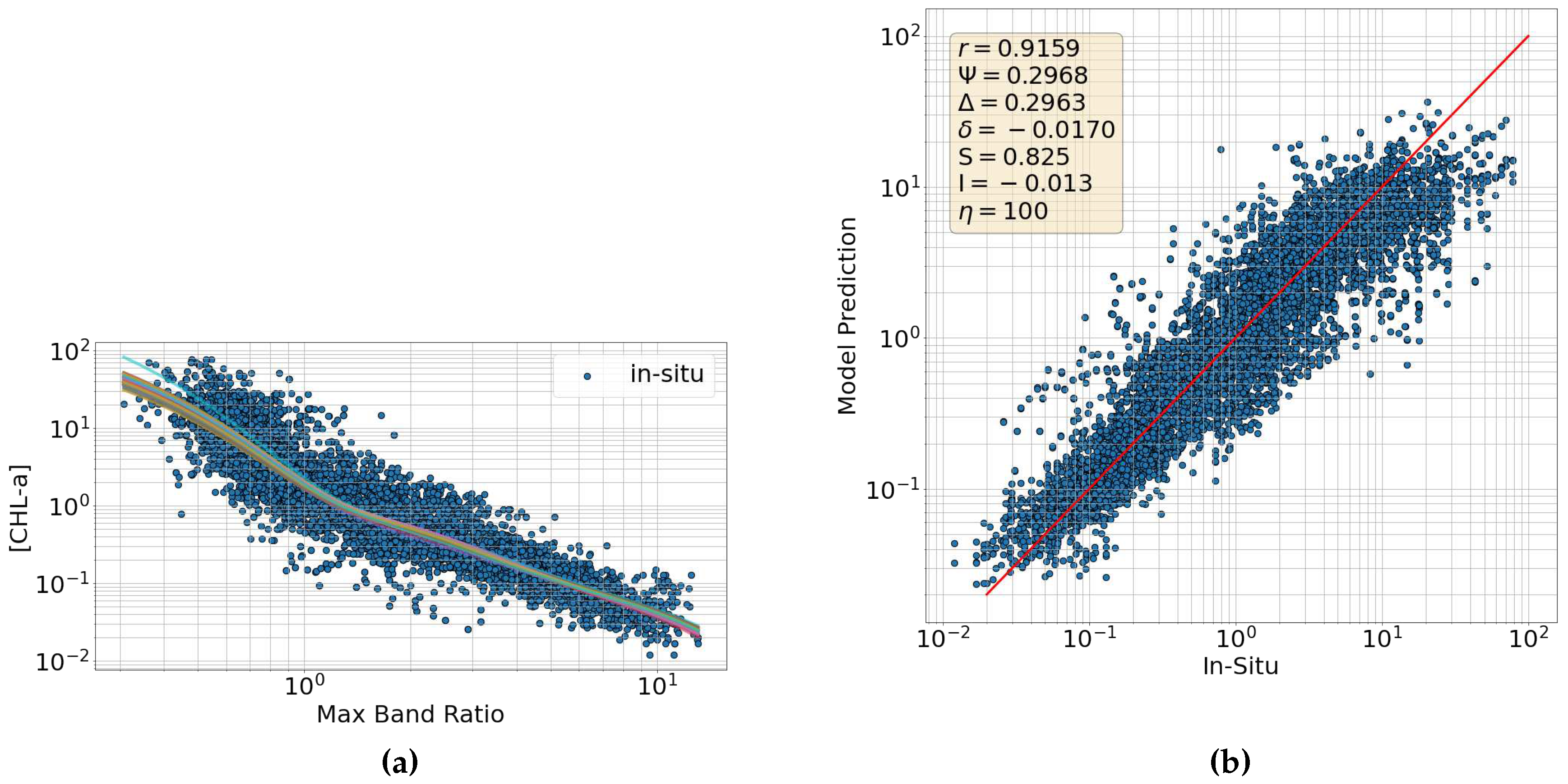
Figure 7.
[CHL-a] observations around the continent of America obtained by propagating MODIS monthly composite remotely sensed reflectances through the (a) MBR-based MAP and (b) OC4 ocean colour model and (c) the corresponding log difference. Four areas of interest are also highlighted, these include the western and eastern coasts of the United States, and the coasts of Mexico and Brazil.
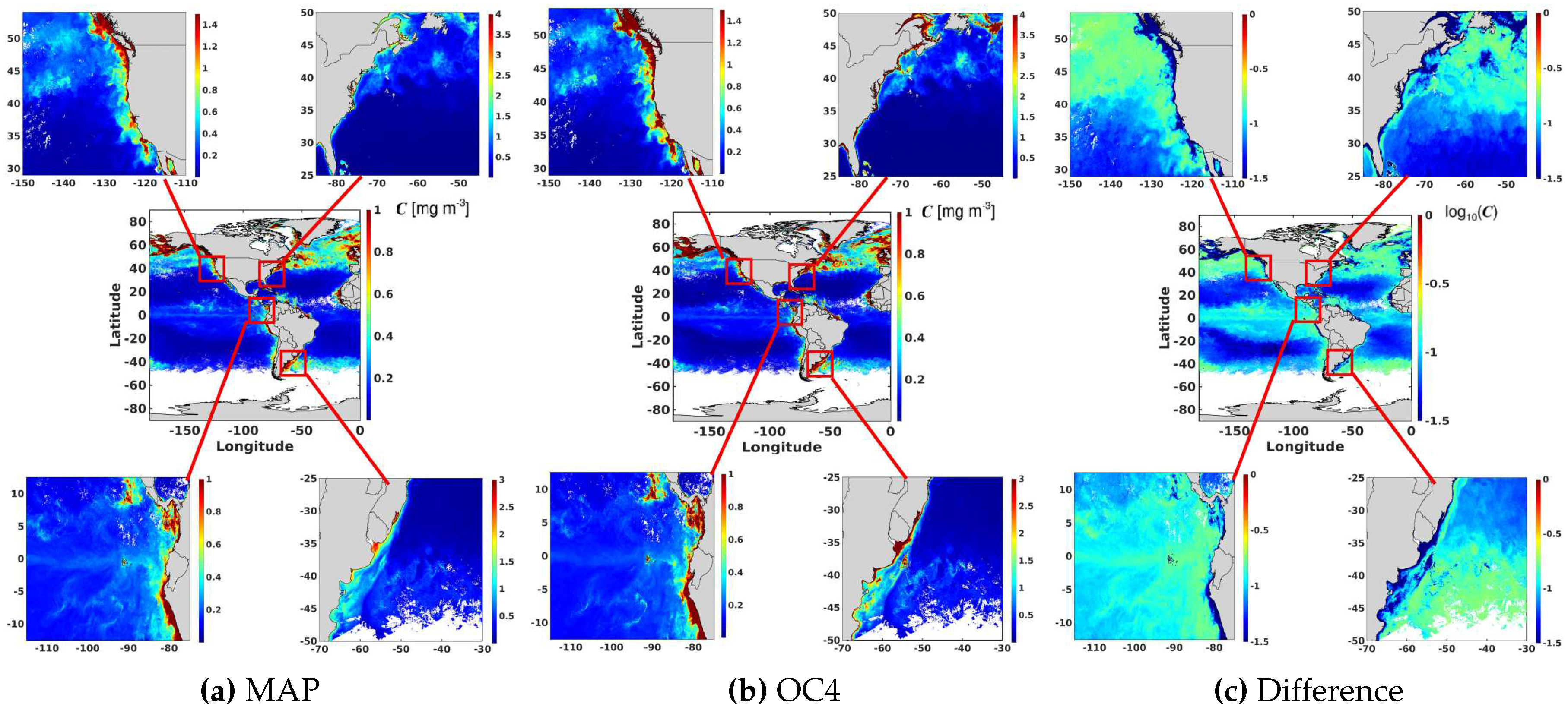
Figure 8.
[CHL-a] observations obtained by propagating MODIS monthly composite remotely sensed reflectances through the (a) MBR-based MAP and (b) OC4 ocean colour models and (c) the corresponding log difference. Four areas of interest are also highlighted.Specifically, the North Sea, the East China Sea and Sea of Japan, and the South African and Indonesian coasts.
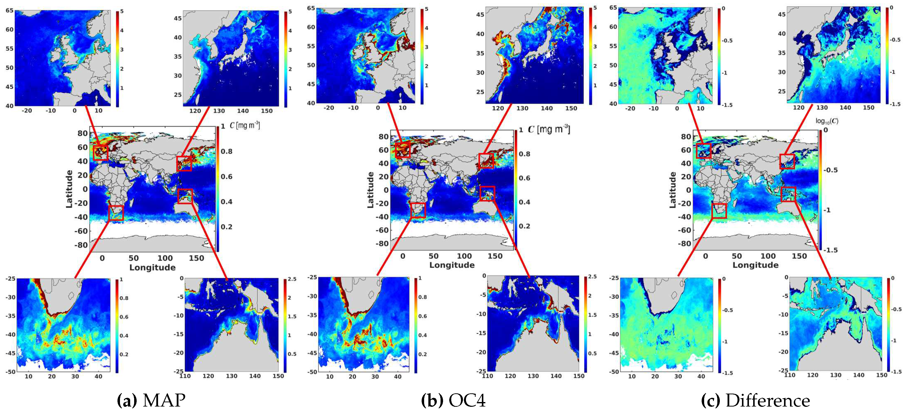
Figure 9.
Daily [CHL-a] image of the southern Red Sea from Sentinel-3 at 300 m spatial resolution: (a) estimated using the MAP and OC4 models alongside their log difference, (b) estimated using OC4, the mean and standard deviation of 100 BNN predicted samples and the corresponding coefficient of variation.
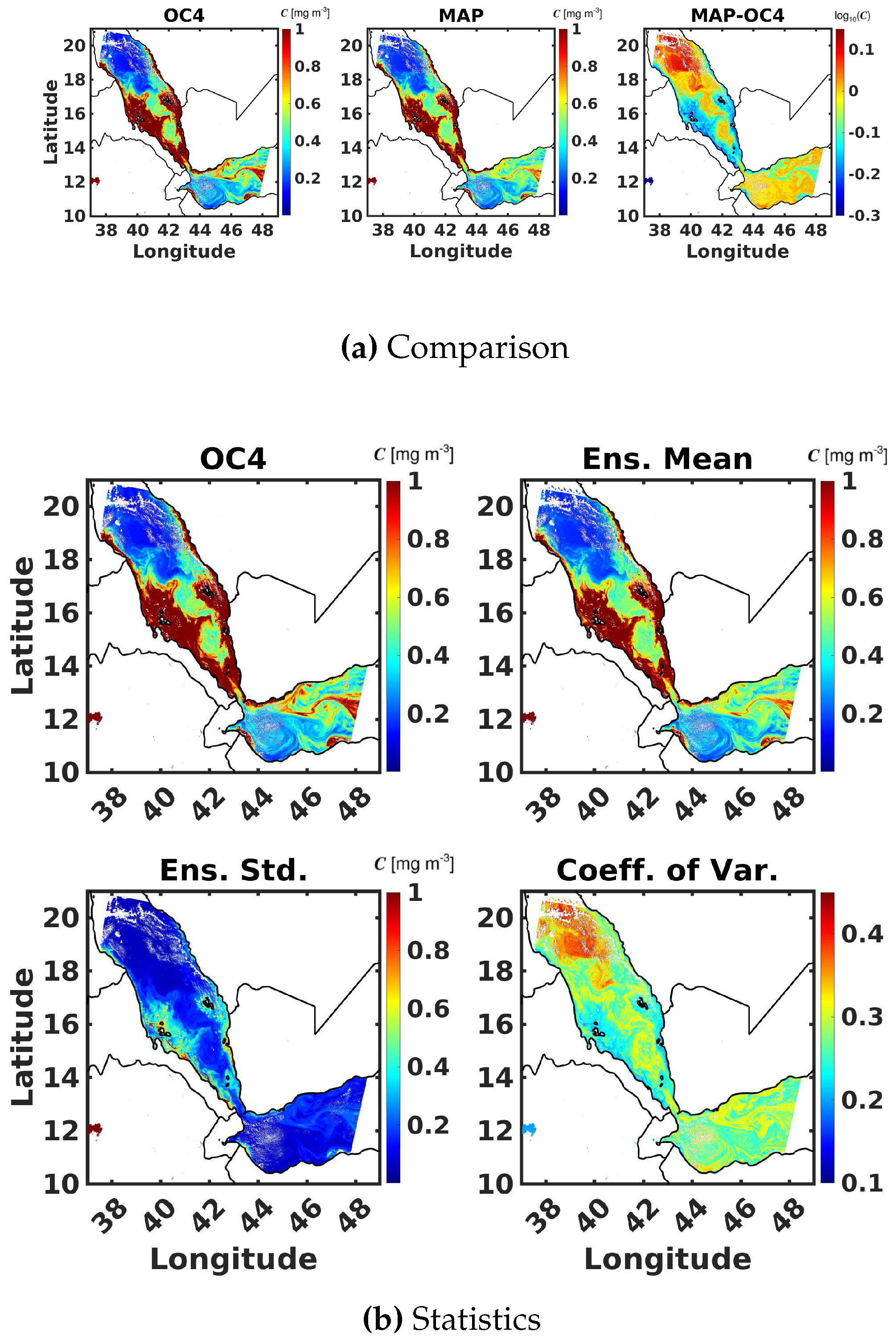
Figure 10.
Comparison of [CHL-a] fields for the Southern Red Sea obtained using the OC4 (top left) model and random samples generated using the BNN model for a single scene retrieved from Sentinel-3 at 300 m spatial resolution.
Figure 10.
Comparison of [CHL-a] fields for the Southern Red Sea obtained using the OC4 (top left) model and random samples generated using the BNN model for a single scene retrieved from Sentinel-3 at 300 m spatial resolution.
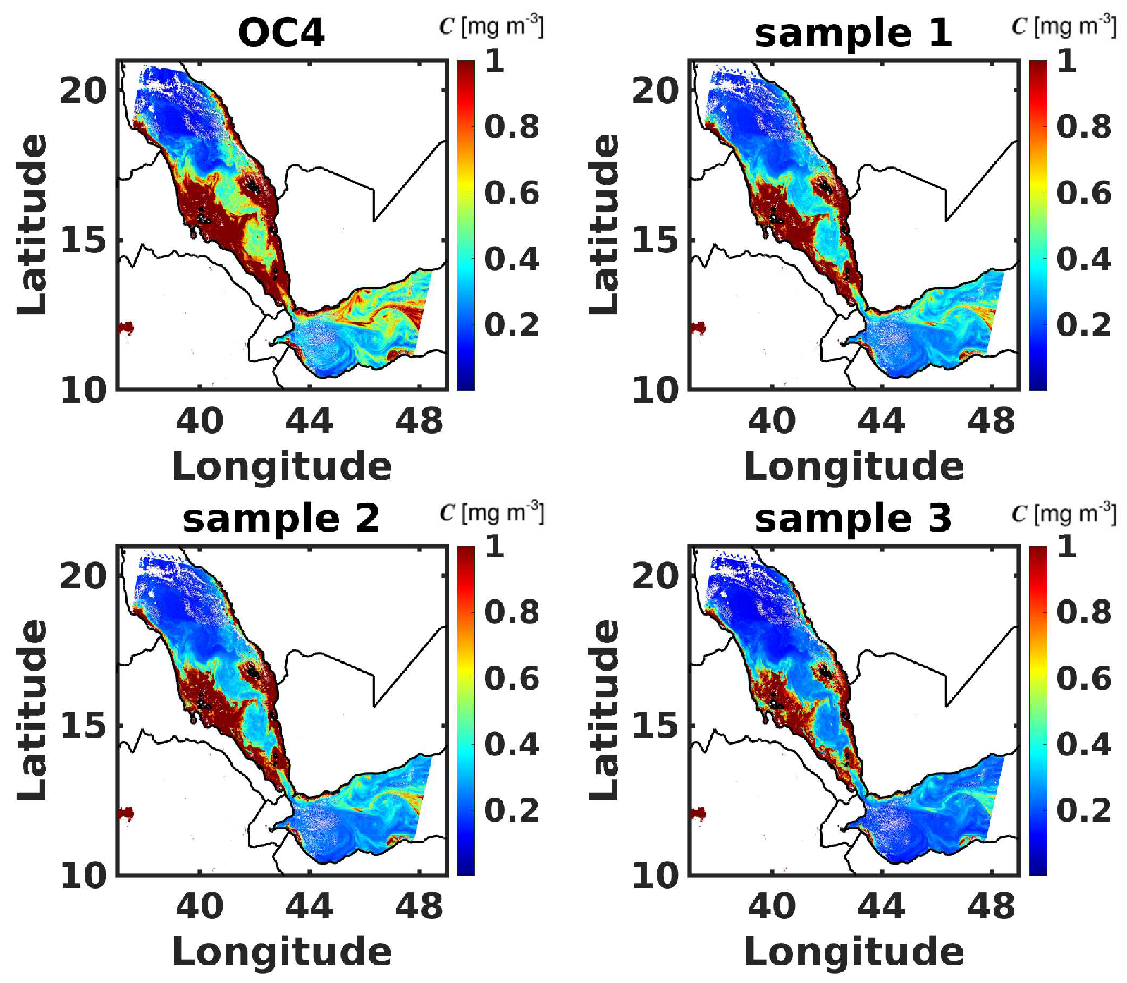
Figure 11.
Daily [CHL-a] image of the Baltic Sea from Sentinel-3 at 300 m spatial resolution: (a) estimated using the MAP and OC4 models alongside their log difference, (b) estimated using OC4, the mean and standard deviation of 100 BNN predicted samples and the corresponding coefficient of variation.
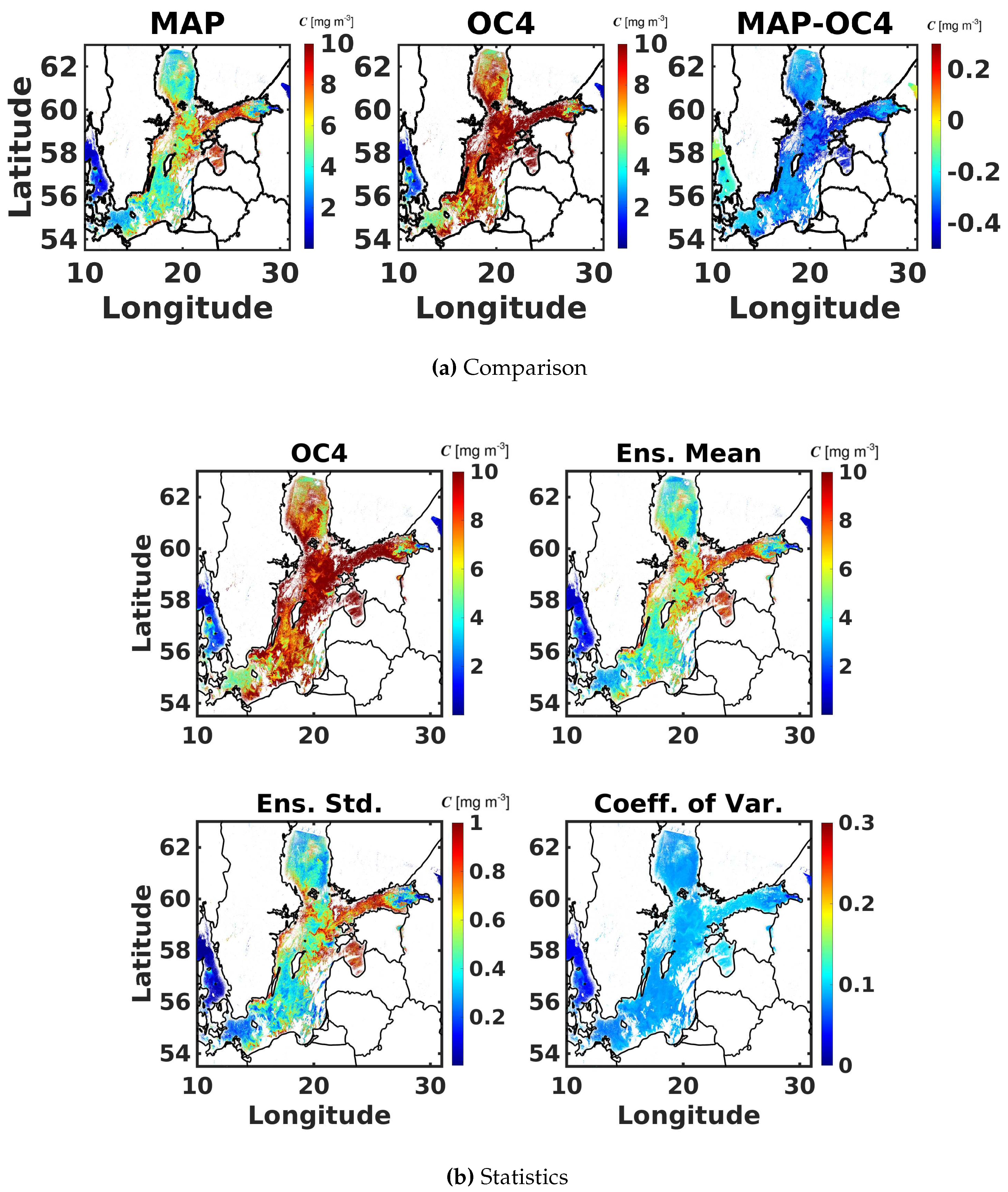
Figure 12.
Daily [CHL-a] image of the northern Red Sea from Sentinel-3 at 300 m spatial resolution: (a) estimated using the MAP and OC4 models alongside their log difference, (b) estimated using OC4, the mean and standard deviation of 100 BNN predicted samples and the corresponding coefficient of variation.
Disclaimer/Publisher’s Note: The statements, opinions and data contained in all publications are solely those of the individual author(s) and contributor(s) and not of MDPI and/or the editor(s). MDPI and/or the editor(s) disclaim responsibility for any injury to people or property resulting from any ideas, methods, instructions or products referred to in the content. |
© 2024 by the authors. Licensee MDPI, Basel, Switzerland. This article is an open access article distributed under the terms and conditions of the Creative Commons Attribution (CC BY) license (http://creativecommons.org/licenses/by/4.0/).
Copyright: This open access article is published under a Creative Commons CC BY 4.0 license, which permit the free download, distribution, and reuse, provided that the author and preprint are cited in any reuse.


