Submitted:
24 January 2024
Posted:
25 January 2024
Read the latest preprint version here
Abstract
This work targets the development of a mobility control system for high-speed series hybrid electric tracked vehicles, which operate with independent traction motors for each track. The scope of the research encompasses the modeling of the series hybrid powertrain specific to military tracked vehicles, as well as an in-depth analysis of their dynamic behavior. Subsequently, the study conducts a critical review of the mobility control approaches sourced from literature, identifying key techniques relevant to high-inertia vehicular applications. Building on the foundational models, the study puts forward a robust closed-loop mobility control system aimed at ensuring precise and stable off-road vehicle operations. The system's resilience and adaptability to a variety of driving conditions are emphasized, with a particular focus on handling maneuvers such as steering and pivoting, which are challenging operations for tracked vehicle agility. The performance of the proposed mobility control system is tested through a series of simulations, covering a spectrum of operational scenarios. These tests are carried out in both offline simulation settings, which permit meticulous fine-tuning of system parameters, and real-time environments that replicate actual field conditions. The simulation results demonstrate the system's capacity to improve vehicular response and highlight its potential impact on the future designs of mobility control systems for the heavy-duty vehicle sector, particularly in defense applications.
Keywords:
Hybrid Electric Tracked Vehicles
; Hybrid Electric Military Vehicles
; Vehicle Control
; Mobility Control System
; Series Hybrid Electric Powerpack
; Tracked Vehicle Dynamics
; Steering Maneuver
; Torque Management
; Robust Control
; Terrain Adaptability
1. Introduction
Tracked vehicles are essential for various sectors, including automotive, defense, construction, and agriculture, due to their superior off-road capabilities. The recent shift towards hybrid electric drive systems similar to those in wheeled vehicles has gained momentum thanks to the advantages they offer. Sivakumar's study states that the hybridization of military vehicles offers significant benefits, including improved fuel efficiency, enhanced drivability and silent running, yet faces considerable development challenges due to the demand for robust and environment-resistant components [1]. Many studies agree on that adding electric power to military vehicles could make them quieter and work better, while also providing extra electric power when needed as summarized in the research that introduces a new hybrid power system for these vehicles that aims to cut down on weight and use less fuel without compromising on how well the vehicle performs [2]. Furthermore, the adaptation of series hybrid drives to tracked vehicles implies a need for distinct controller requirements: a power management algorithm for effective power distribution among the power sources (battery and generator set) and a mobility control algorithm for independent motor operation to achieve desired motion control variables, including sprocket velocity and track speed differential during maneuvers.
FNSS, a global leader in the land systems sector, is at the forefront of this innovation, not only producing wheeled and tracked armored combat vehicles, turrets, and engineering vehicles but also exploring hybrid powertrain technologies [3]. The focus of this study revolves around the hybridization of an FNSS armored tracked vehicle named KAPLAN HYBRID, as shown in Figure 1. The hybridization work is presented at EVS36 symposium in Sacramento, USA, in June 2023 by Çeliksöz together with the publication of conference paper in which control system development of the vehicle is focused on [4]. This paper extends the conference paper and reports the development of a mobility control system specifically tailored for FNSS's series hybrid tracked vehicles. The approach commences with the modeling of vehicle dynamics and hybrid powertrain using MATLAB Simulink, followed by a review of existing mobility control strategies detailed in the literature. Subsequently, in the simulated environment, a robust closed-loop mobility control system is designed and tested, while the power management system is analyzed as a black box model that sets instantaneous traction power limits to ensure clarity and maintain focus on mobility controller development. The robustness of this system is validated by simulating the vehicle model against diverse dynamic traction power constraints in various scenarios.
Before discussing the details of this work, it is important to note that current literature documents a range of control methodologies for hybrid systems in the following manner. Research of Ze-yu et al. implements a BP Neural Network combined with a PID algorithm to refine the vehicle's steering control [5]. Even though the traction motor torques are initially defined by the neural network, the introduction of PID adjustments accommodates variable terrain coefficients. Hu et al. discuss a dual-motor drive strategy that innately computes torques for a predesignated target turning radius and employs a PID controller to achieve the radius more rapidly [6]. Additionally, Pei et al. proposed a Torque fuzzy compensation control strategy to enhance steering execution, where torque distribution is regulated by applying direct multipliers derived from fuzzy logic [7], and the corresponding diagram is illustrated in Figure 2. In short, hybrid electric tracked vehicle control system researches are based on manipulating the sprocket torques to achieve lateral motion together with longitudinal.
The current study aims to not only synthesize the existing body of research but also to push the boundaries through the development of a mobility control system for FNSS's own series hybrid tracked vehicles. The primary contributions and conclusions of this work emphasize the technological advancements in hybrid drive systems for tracked combat vehicles and their implementation, setting the stage for future research and practical applications in the field.
Moreover, the study provides a comprehensive evaluation of the system's performance under a variety of combat scenarios, ensuring that the vehicles are equipped to handle diverse and challenging terrains. Discussions included are not limited to theoretical assessments; they also present insights from extensive field tests that enhance the practical feasibility and dominance of the hybrid system.
2. Materials and Methods
The plant and control system models are deliberately designed to further research initiatives and assess the algorithm's performance with a variety of control inputs and driving cycles. The plant modeling incorporates power sources, the traction system, and the vehicle's framework, whereas the control system is explored in terms of power management and mobility control systems. These modeling activities are carried out distinctly for the plant and control systems, with this division to enable the examination of diverse vehicle configurations and powertrain systems. After each section is individually shaped, they are unified to construct an integrated model depicted in Figure 3. A more detailed explanation of each model is provided in the following sections, offering a deeper insight into how each component functions within the entire system.
2.1. Modeling the Plant: Hybrid Electric Tracked Vehicle
In this section, attention is given to the modeling process for the hybrid electric tracked vehicle's plant. The focus here is on the representation of hybrid electric propulsion systems specific to tracked vehicles and modeling techniques that capture the dynamic relationships between the traction system components and the vehicle's overall architecture. Furthermore, power sources are briefly defined even though the scope of this work is powertrain and mobility of the vehicle other than energy management.
2.1.1. Electric Traction System
The electric traction system, which is presented in a simplified schematic in Figure 4, is modeled through a composite approach that brings together the electric motors, gearboxes, and friction brakes connected to left and right sprockets. This configuration is carefully constructed to accurately reflect the system's mechanical and electrical interactions, ensuring that the model provides a realistic representation of the vehicle dynamics.
In the given configuration, the e-motors are modeled as a source of torque featuring a unity transfer function, which means an absence of delay in the torque delivery upon request, as long as it doesn't exceed the motor's torque reserve. To maintain this behavior, the smaller of the requested torque or available torque at the current shaft speed is used, as illustrated in equation (1). Subsequently, the torques generated by the motors are scaled by the gear ratio and modified for gearbox efficiency.
Tout,Motor = min{Tavail,Motor (w), TRequest}
In the equation (1); Tout,Motor, Tavail,Motor (w) and TRequest represents motor torque output, speed dependent available motor torque and requested torque via mobility control system respectively. The speed dependent available motor torque is obtained from full load curve which represents speed-torque characteristics of the electric motor. Even though the full load curve is distinct to electric motors, it displays a standard trend: a constant torque at lower speeds transitioning to a constant power at higher speeds. This pattern is elaborated on in Aiso's research, as exemplified in Figure 5 [8].
Prior to transitioning to the vehicle dynamics calculations, the torques from the friction brakes are combined with those from the gearbox output, as shown in equation (2). The resulting torque is then supplied to the subsystem governing the dynamics of the tracked vehicle.
TSprocket = iGB ηPT Tout,Motor - TBrake
In the equation (2); TSprocket, iGB, ηPT and TBrake represent sprocket torque output, gear ratio, powertrain efficiency and applied brake torque respectively.
2.1.2. Dynamics of the Tracked Vehicle
The dynamics of the tracked vehicle are captured using a 3-DOF (degrees of freedom) vehicle model that considers the equations of motion along the longitudinal (x), lateral (y), and yaw (z) axes, which are detailed in Figure 6 for a left maneuver. Equations (3), (4), and (5) are derived for this maneuver assuming a center of gravity in the middle of lateral axis unlike longitudinal.
mVhc ax = (FTraction,left – FResistance,left) + (FTraction,right – FResistance,right) = ΣFx,i
mVhc ay = (QLateral,left + QLateral,right) xcenter,rear - (QLateral,left + QLateral,right) xcenter,front = ΣFy,i
IVhc,zz Φ’ = ΣFx,i yResultant – ΣFy,i xResultant
In expressions the terms mVhc, IVhc,zz, ax, ay, and Φ’ denote the mass of the vehicle, inertia about the vertical axis at the vehicle's center of gravity, accelerations in the longitudinal and lateral directions, and the rate of yaw, respectively. The forces FTraction,left, FTraction,right, FResistance,left, and FResistance,right are indicative of the traction and longitudinal resistance forces acting on the vehicle for left and right tracks respectively. While QLateral,left and QLateral,right characterize the distributed side frictional forces per length interacting with the left and right tracks, lateral distance between vehicle’s cog (center of gravity) and vehicle’s front and rear end are denoted by xcenter,front and xcenter,rear. Furthermore, the net forces along the longitudinal and lateral axes are given by ΣFx,i and ΣFy,i, with the corresponding distances from these net forces to the vehicle's center of gravity being represented by xResultant and yResultant correspondingly.
Dynamic calculations are followed by integrations of computed accelerations to obtain speed components of the vehicle in longitudinal, lateral and yaw axes.
2.1.3. Power Sources
Power sources of the hybrid vehicle are combination of battery and generator set involving diesel engine and electric generator. In this work, it is assumed that the available power, the summation of power sources’ reserve, is constant for clear investigation of mobility control system.
2.2. Mobility Control Method
- Control Theory and Big Picture
Based on the research and findings presented in previous sections, it is found that the vehicle in question, a high-speed off-road military vehicle, requires a strong and effective closed-loop control system to achieve the targeted maneuverability at high speeds across various terrains. It has been determined that while producing the overall torque in response to the driver’s input is correlated with accelerator pedal position, the distribution of the torque should be adjusted based on the feedback from the speed difference between the sprockets. This differential is directly related to the angle of the steering wheel set by the driver. In other words, a certain speed differential between the electric motors is decided, corresponding to the given steering wheel angle, through the employment of the closed-loop controller. The strategy for mobility control can be seen in Figure 7, demonstrated via block diagrams. There are four primary subsystems, each with special roles. The Driver block is designed to feed in specific driver commands for varying test runs and is separate from the onboard vehicle control system. The Driver command preprocessor and the closed-loop controller blocks are critical to the control system, handling the computational side of mobility control and transforming driver instructions into specific torque demands for the left and right motors. Lastly, the traction system represents the plant including mathematical models of the electric motor and gearbox. The outputs from the traction system are the torques delivered to the left and right sprockets, which are main inputs of the vehicle dynamics model.
- Preprocessing and Shaping Control Commands
Within the Driver Command Preprocessor section, throttle and steering inputs are preprocessed depending on the selected gear and current vehicle speed. The shaping of the inputs is performed by three main functions: Throttle shaping, steering shaping and pivot shaping.
The throttle shaping function is developed to adjust the input received from the accelerator pedal based upon the selected vehicle mobility mode, with the objective of improving the driver's experience. This is achieved by mapping the position of the pedal to specific throttle values, which correspond to a range of distinct operational modes, as depicted in Figure 8.
In scenarios where safety is significant, such as in the preliminary testing phase of the algorithm, a conservative throttle response is preferred. This scenario is optimally supported by a shaping function similar to option 1 in Figure 8, which is characterized by a more gradual and controlled acceleration curve. On the other hand, for circumstances that demand a more robust and dynamic performance, such as during an aggressive driving test, the shaping curve should approach option 3 in Figure 8. This latter option is fine-tuned to yield a sharper and more immediate increase in throttle response, reflecting the vehicle's need for rapid acceleration.
Throughout the majority of testing protocols and simulation exercises, option 2, which represents a linear throttle shaping, is the preferred choice. This option is beneficial because it provides a straightforward correlation between pedal input and throttle output. Such predictability is essential for conducting a clear and systematic analysis of other control subsystems. It enables control engineer to isolate and evaluate the performance characteristics of each subsystem without the added complexity that non-linear shaping options might introduce.
Steering shaping function targets to transform steering commands into differences in motor velocities through a suitable shaping strategy. FNSS has compiled test records from standard tracked vehicles for calibration purposes. Upon analyzing the change in speed at maximum steering, a pattern is noted where the difference in speed across the motors at full steer changes with vehicle velocity. However, this increase is interrupted by sudden changes at certain velocities, making the pattern non-linear. Closer inspection shows that these dips coincide with the gear shifting points of traditional gearboxes. For a consistent steering behavior, a smooth curve is mapped over the test data, excluding these dips. The normalized version of this test data together with the smoothing curve is depicted in Figure 9, ensuring confidentiality.
The pivot maneuver is executed through a specifically designed shaping function. Initially, the maximum speed range is established. Subsequently, the position of the accelerator pedal is correlated to this range to achieve the required speed differential. In addition, the angle of the steering wheel is utilized to decide the pivot turn's direction, allowing the driver to command a counter-clockwise (CCW) or clockwise (CW) rotation by steering, regardless of the actual degree of the wheel's turn. The plot for this pivot shaping strategy can be found in Figure 10, providing a visual representation of the maneuvering process.
By employment of these shaping functions, total cumulative torque demand and desired speed difference variables are designated. Based on these desired inputs, a closed loop motion controller is operated and torque demands of left and right traction motors are determined.
2.3. Power Management Method
The mobility control system serves a dual purpose within the vehicle's control architecture. Primarily, it is responsible for directly actuating the traction motors. However, the scope of the mobility control system's functionality extends to playing an important role in the vehicle's overall power management by continuously monitoring the instantaneous power requirements of the traction system.
As the vehicle operates, the mobility control system calculates the immediate power demands needed for traction by multiplication of torque demand, measured speed and corresponding traction efficiency. Once the power calculations are performed, the mobility control system communicates a traction power request to the power management algorithm which is another significant system of the hybrid tracked vehicle in question as explained in the work of Akar et al. [9].
This request for power is carefully evaluated to control how the power management system should regulate the generator set's output. By providing this traction power request, the mobility control system ensures that the power management system can adjust the generator's output dynamically, matching the generated power with the traction system's demands. This synchronous operation is crucial for ensuring that the difference between generated and demanded power does not exceed the limits of electric battery.
3. Simulations and Results
Using the modeling approach and equations mentioned previously, mobility control system is developed and simulated using MATLAB Simulink. An overview of the Simulink model is illustrated at Figure 11.
The functional scenarios that include pivot maneuvers, steering actions, forward and reverse movements are studied by extensive simulations in order to analyze the vehicle's behavior under various operational conditions. To analyze the results, a simulation postprocessing interface has been developed, which permits the in-depth observation of the vehicle's motion dynamics and the associated responses from the powertrain, including variables like sprocket torques and track speeds.
An example of this simulation platform can be seen in Figure 12, which specifically illustrates the interface during a scenario involving a forward steering motion at a predetermined longitudinal speed of the vehicle. In this particular simulation, it is observed that upon reaching the 50th seconds of the simulation time, the driver introduces a steering command, inputting a 40% steering angle into the system. Due to this action the motor torques experience a substantial and rapid increase. After this initial jump in torque, caused by the need to adjust the vehicle's trajectory according to the steering input, the motor torque levels exhibit a stabilization, converging to a steady-state value. Steady-state torques involved in steering are now balanced, and the vehicle is maintaining the new desired directional path at a constant speed.
Additionally, Figure 13 indicates that the speed differential between the left and right electric motors reaches the preset target specified by the steering shaping function. An upward trajectory in speed difference is observed as the steering input rises, a response predicted from the closed-loop control system. The presence of noise in the actual speed differential originates from the particular characteristics of the electric motors' encoders. It is assumed that the encoders are influenced by white noise to test the controller's capability to cope with this type of disturbance.
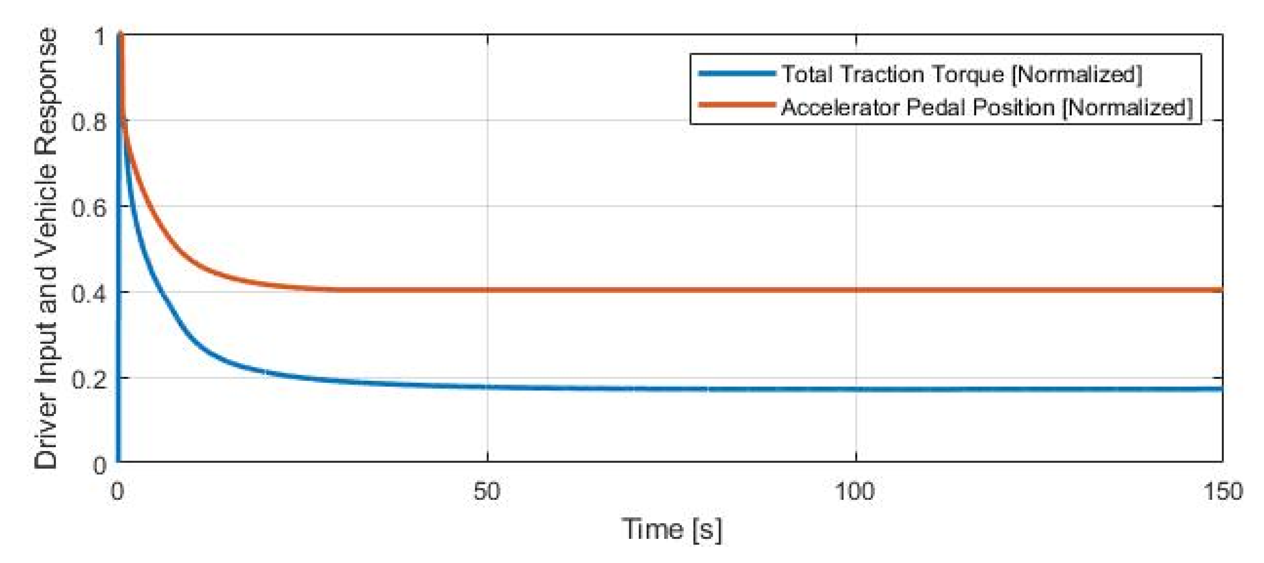
Observations of the vehicle's longitudinal response are demonstrated via Figure 14 as well. It is noted that there is a proportional increase in the vehicle's total torque correlating with the rise in the accelerator pedal position, regardless of the steering input. This effect is realized by applying a linear throttle shaping function as explained in the mobility control system section.
4. Discussion and Conclusion
This document investigates the mobility control system of a series hybrid electric tracked vehicle. The objective of the system is to control the electric motor torques to produce the entire torque demanded by the throttle, while achieving the necessary speed differential when steering inputs are made. Traditional testing methods on the electrified tracked vehicle helped establish the speed differential target.
Results from practical demonstrations indicate that the intended motion is achievable with the deployed mobility control system. Moreover, the speed differential methodology enhances system adaptability across varying terrains. Even though different friction coefficients may necessitate varied sprocket torques for steering actions, the employment of a closed-loop speed differential strategy yields the correct sprocket torques. Variations in radius due to changes in slip characteristics are compensated by the driver's input, effectively incorporating human interaction as part of the loop.
The integration of regenerative braking into the series hybrid system further demonstrates the potential for increased efficiency and reduced wear on braking components. By converting kinetic energy into electrical energy during deceleration phases, energy is fed back into the battery, thus extending the operational range of the vehicle. Initial tests exhibit promising results, with noticeable energy recovery without compromising the stability or control of the vehicle. The interaction between regenerative braking and torque distribution algorithms is crucial; it maintains driving dynamics that are consistent with driver expectations. This addition to the mobility control system complements the existing architecture, presenting a beneficial approach to vehicle energy management and efficiency optimization.
Overall, the mobility control system represents a significant advancement in the management of series hybrid electric tracked vehicles, and future refinements could be made to fine-tune the relationship between driver inputs and vehicle performance, supporting the human-machine interface for optimal control.
Author Contributions
Conceptualization, D.Ç. and V.K.; methodology, D.Ç. and V.K.; software, D.Ç.; validation, D.Ç. and V.K.; formal analysis, D.Ç. and V.K..; investigation, D.Ç. and V.K.; resources, D.Ç. and V.K.; data curation, D.Ç. and V.K.; writing—original draft preparation, D.Ç.; writing—review and editing, D.Ç. and V.K.; visualization, D.Ç. and V.K.; supervision, D.Ç. and V.K.; project administration, D.Ç. and V.K.; funding acquisition, D.Ç. and V.K. All authors have read and agreed to the published version of the manuscript.
Funding
This work was carried out in Hybrid Electric Tracked Vehicle Development project of FNSS Savunma Sistemleri A.Ş. and the work is fully funded by FNSS Savunma Sistemleri A.Ş.
Data Availability Statement
The data and software materials of this research are owned by FNSS Savunma Sistemleri A.Ş. and cannot be shared due to confidentiality policies of the company.
Acknowledgments
Our thanks go to the R&D Team at FNSS Savunma Sistemleri A.Ş. whose assistance was crucial in completing this work.
Conflicts of Interest
The authors declare no conflict of interest.
References
- Sivakumar, P.; Venkatesan, G.; Viswanath, H. Configuration Study of Hybrid Electric Power Pack for Tracked Combat Vehicles. Defence Science Journal 2017, 67, 354–359. [Google Scholar] [CrossRef]
- Randive, V.; Subramanian, S.C.; Thondiyath, A. Design and analysis of a hybrid electric powertrain for military tracked vehicles. Energy 2021, 229. [Google Scholar] [CrossRef]
- FNSS. Available online: https://www.fnss.com.tr/en (accessed on 6 November 2023).
- Çeliksöz, D.; Kılıç, V. Motion Control System Development of Serial Hybrid Electric Tracked Vehicles. 36th International Electric Vehicle Symposium and Exhibition (EVS36), Sacramento, California, USA, 11-14 June 2023.
- Ze-yu, C.; Cheng-ning, Z. Control strategy based on BP neutral network plus PID algorithm for dual electric tracked vehicle steering. 2nd International Conference on Advanced Computer Control, Shenyang, China, 27-29 March 2010. 29 March. [CrossRef]
- Hu, J.; Tao, J.; Zhao, W.; et al. Modeling and simulation of steering control strategy for dual motor coupling drive tracked vehicle. Journal of the Brazilian Society of Mechanical Sciences and Engineering 2019, 41. [Google Scholar] [CrossRef]
- Pei, L.; Yan, J.; Tu, Q.; et al. A Steering Control Strategy Based on Torque Fuzzy Compensation for Dual Electric Tracked Vehicle. Filomat 2018, 32. [Google Scholar] [CrossRef]
- Aiso, K.; Akatsu, K. Performance Comparison of High-Speed Motors for Electric Vehicle. World Electr. Veh. J. 2022, 13, 57. [Google Scholar] [CrossRef]
- Akar, A.; Çalık, G.; Çeliksöz, D. Battery Sizing & EV Mode PMU Algorithm In Military Armored Hybrid Electric Vehicles. 36th International Electric Vehicle Symposium and Exhibition (EVS36), Sacramento, California, USA, 11-14 June 2023.
Figure 1.
KAPLAN HYBRID, Developed by FNSS [3]
Figure 1.
KAPLAN HYBRID, Developed by FNSS [3]
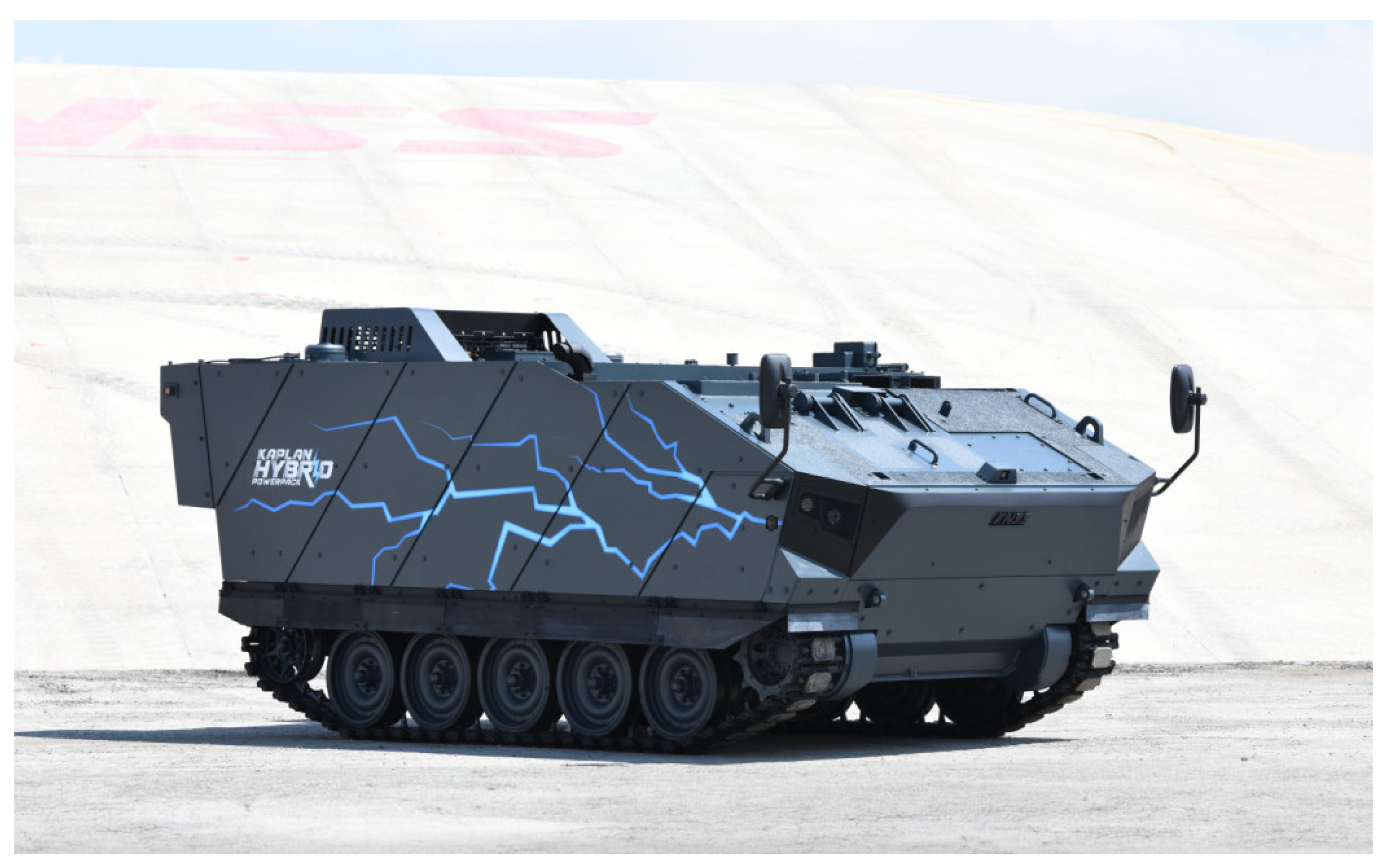
Figure 2.
Torque fuzzy compensation control strategy [7]
Figure 2.
Torque fuzzy compensation control strategy [7]
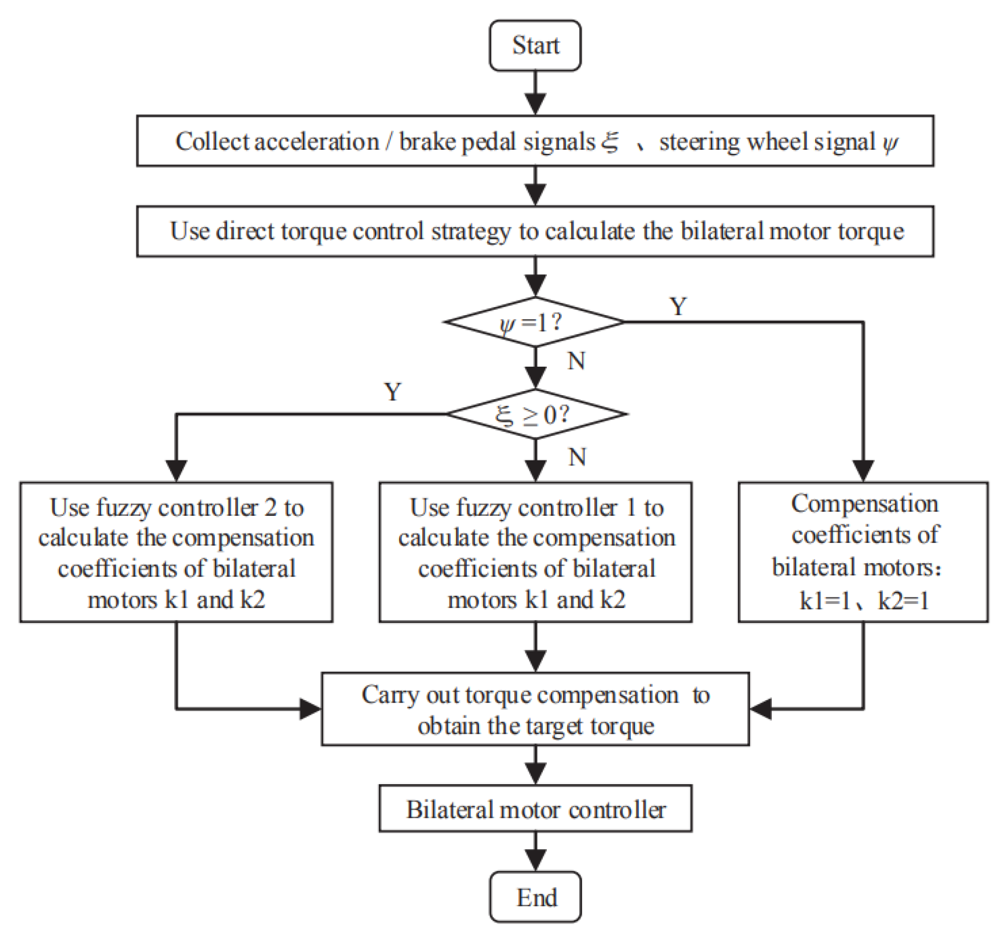
Figure 3.
Block Diagram of the Hybrid Tracked Vehicle Model and Controller
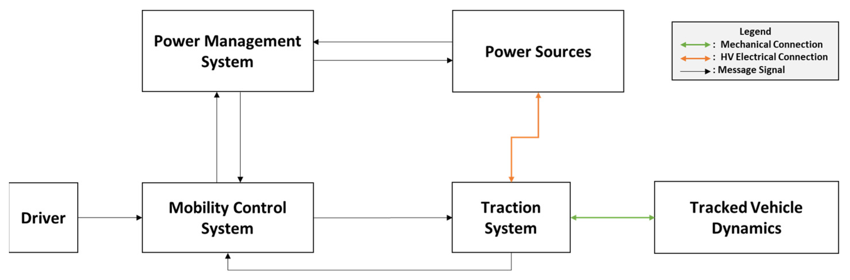
Figure 4.
Schematic of Electric Traction System
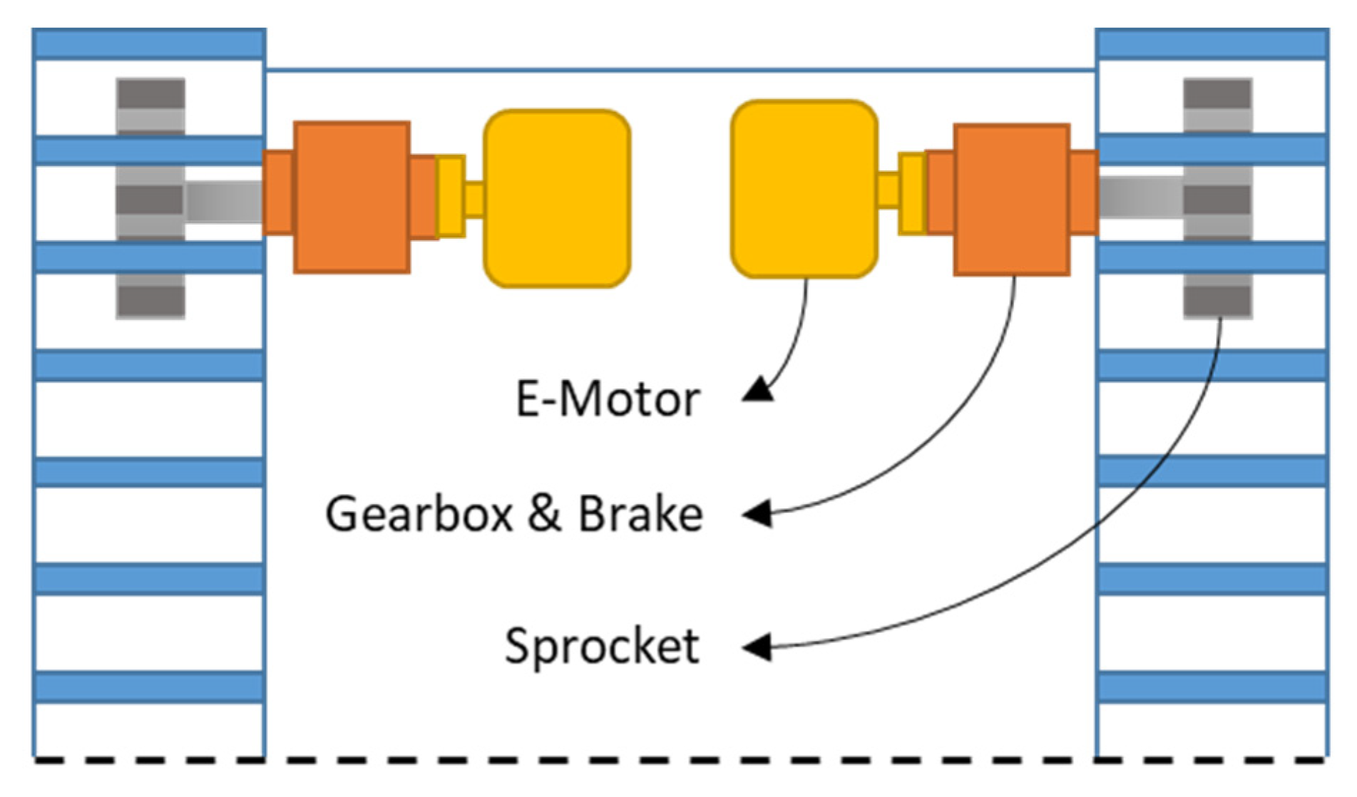
Figure 5.
Full Load Characteristic Curve for an Electric Motor [8]
Figure 5.
Full Load Characteristic Curve for an Electric Motor [8]
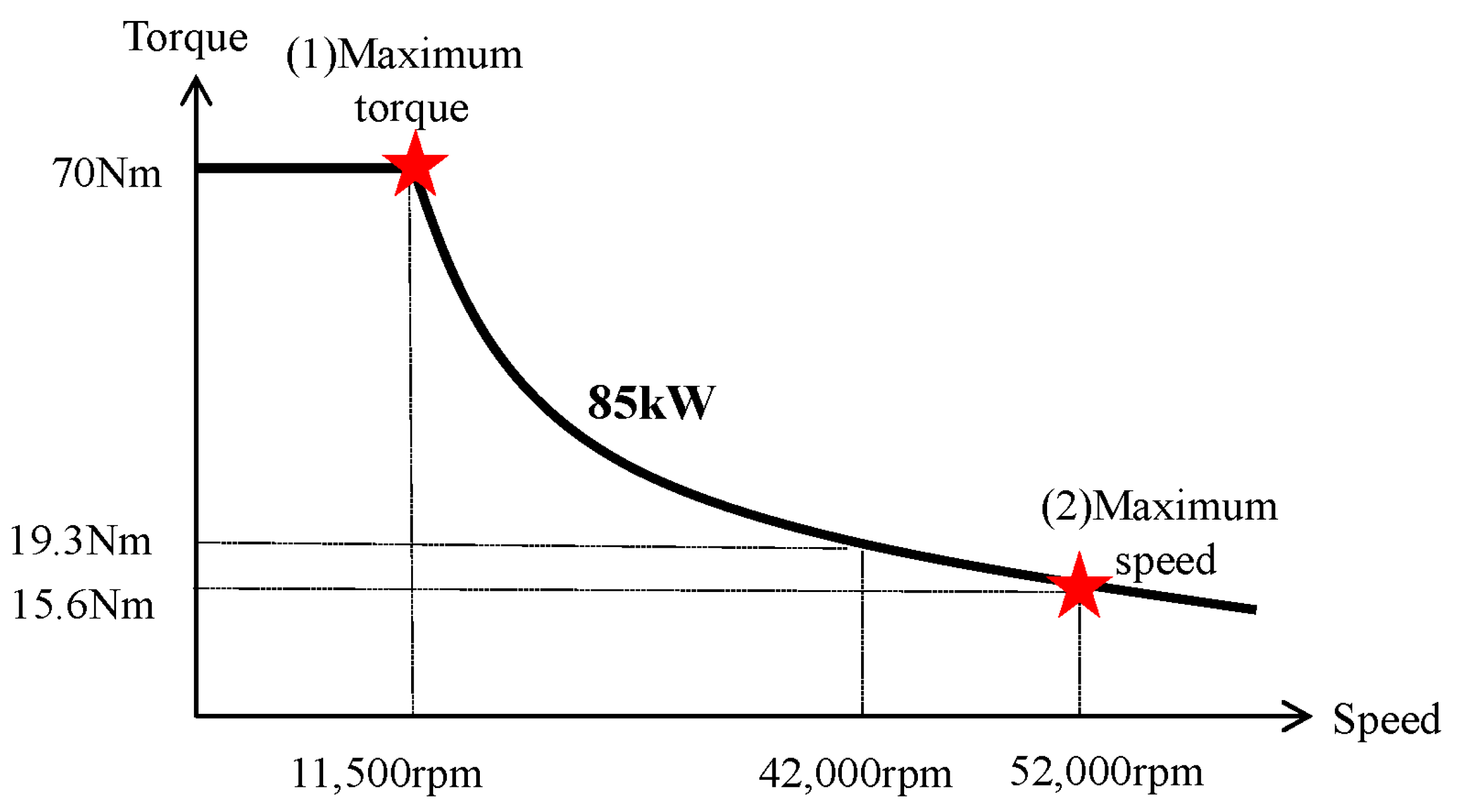
Figure 6.
Loads on a tracked vehicle during left maneuver
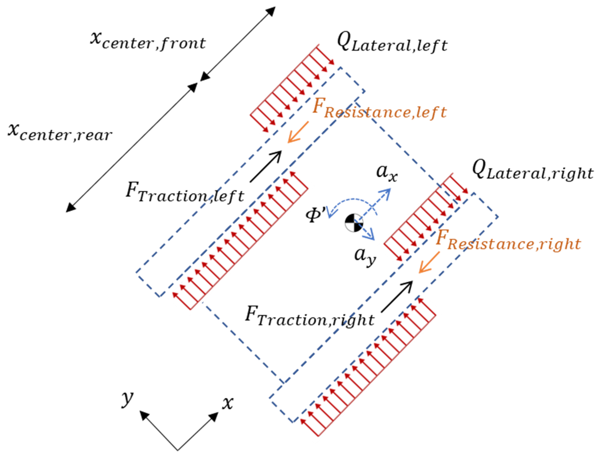
Figure 7.
Big Picture of Mobility Control System
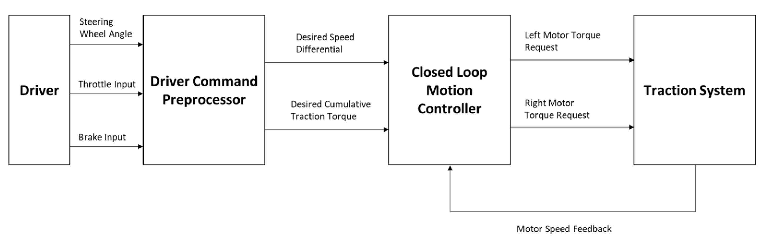
Figure 8.
Throttle Shaping Options
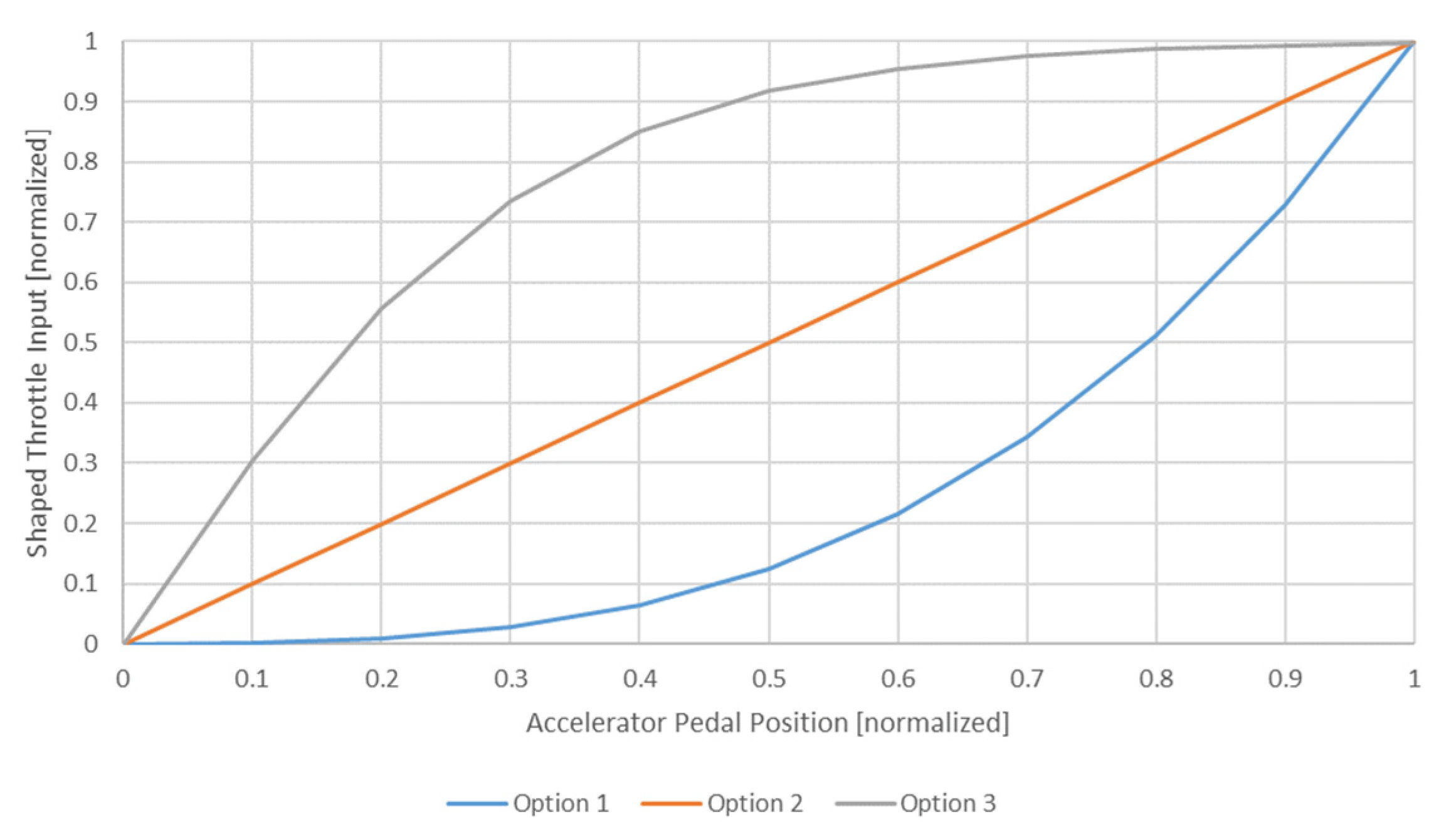
Figure 9.
Steering Shaping Strategy in Normalized Form
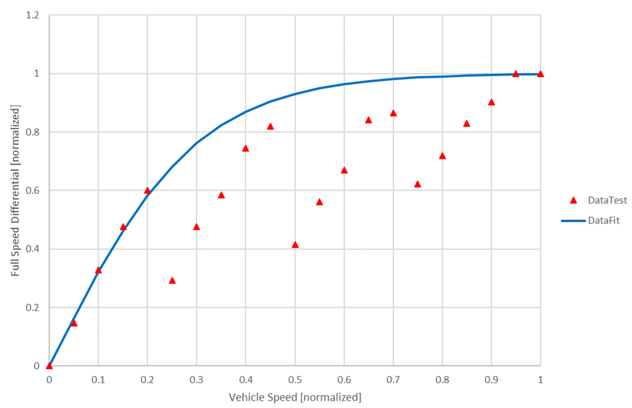
Figure 10.
Pivot Shaping Strategy in Normalized Form
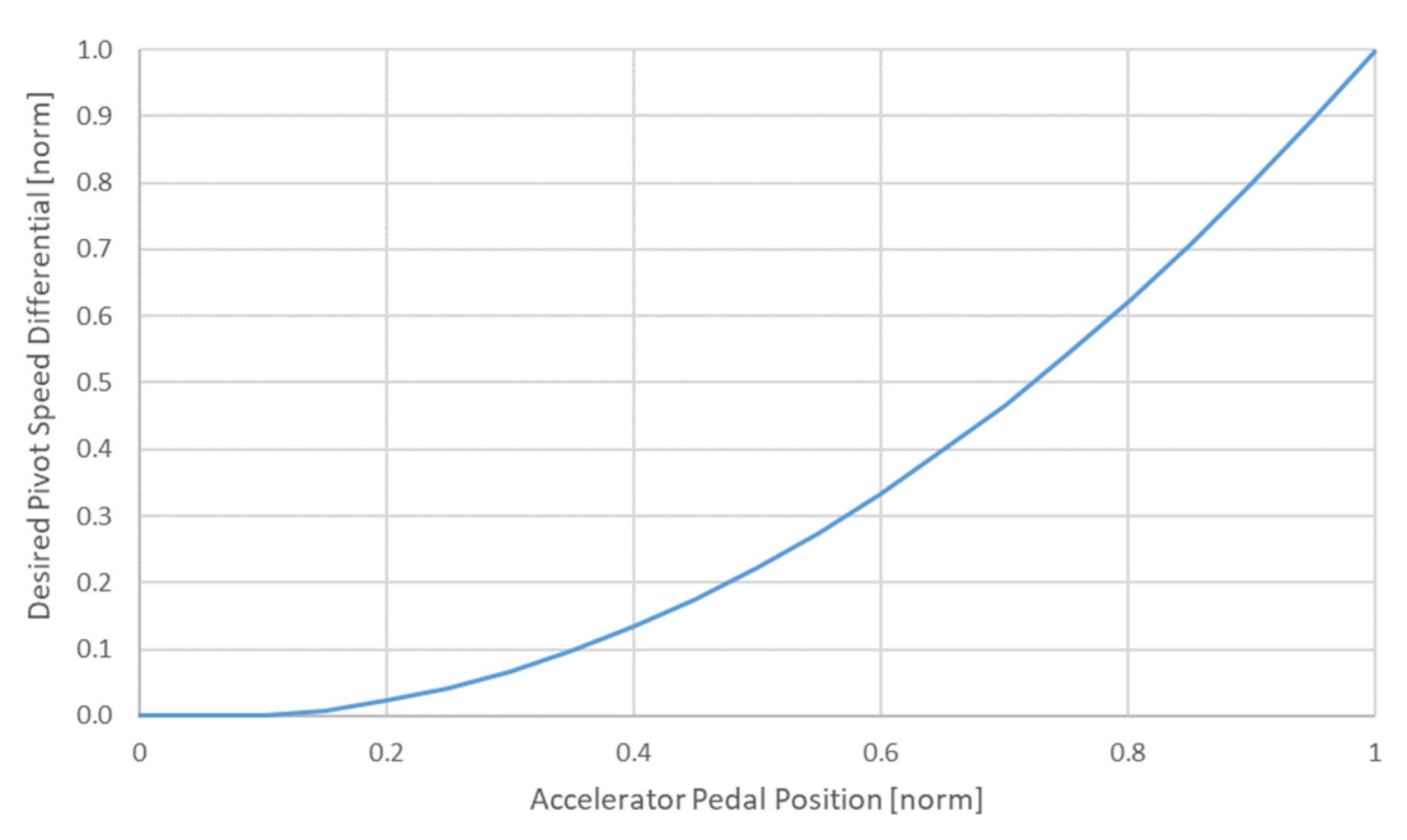
Figure 11.
Simulink Model of the Hybrid Tracked Vehicle
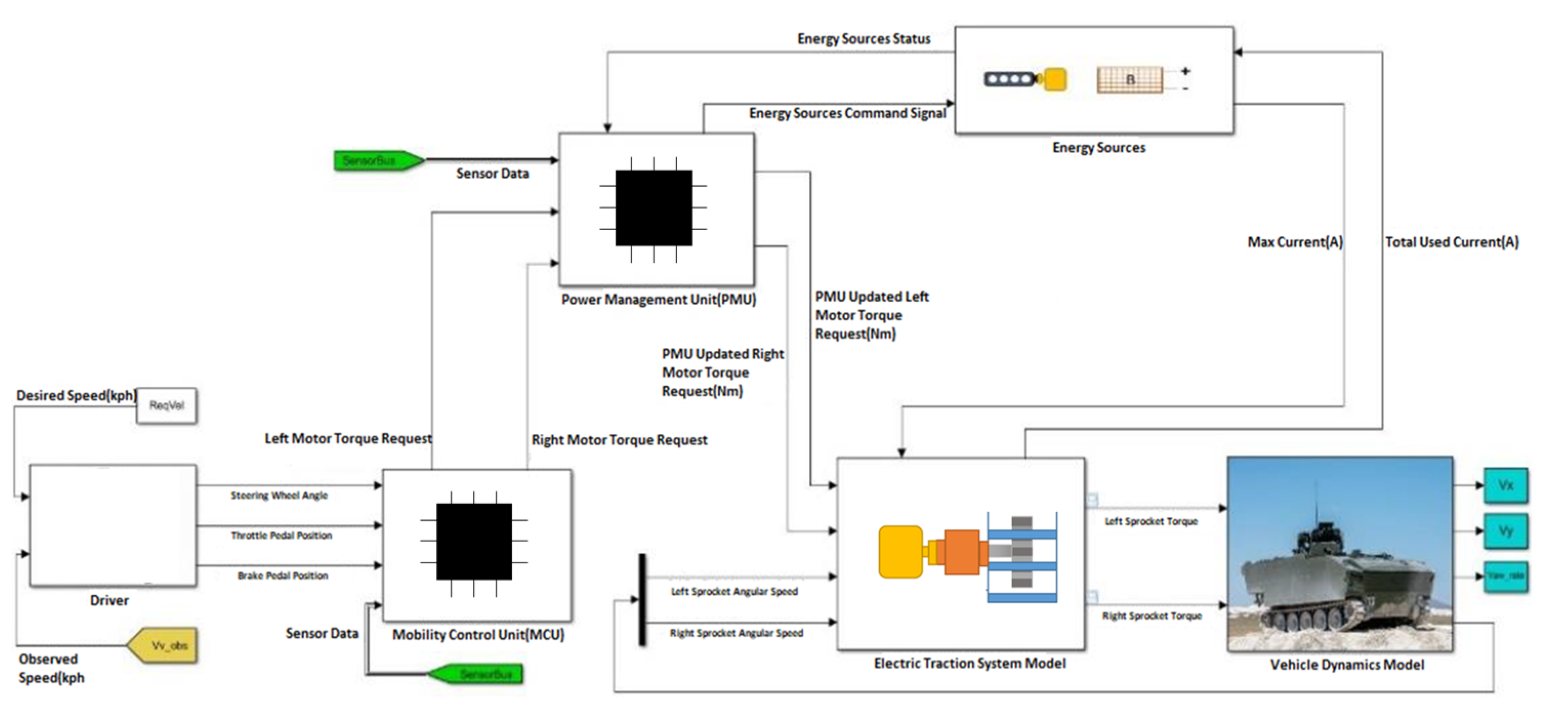
Figure 12.
Simulation Interface for a Cornering Maneuver
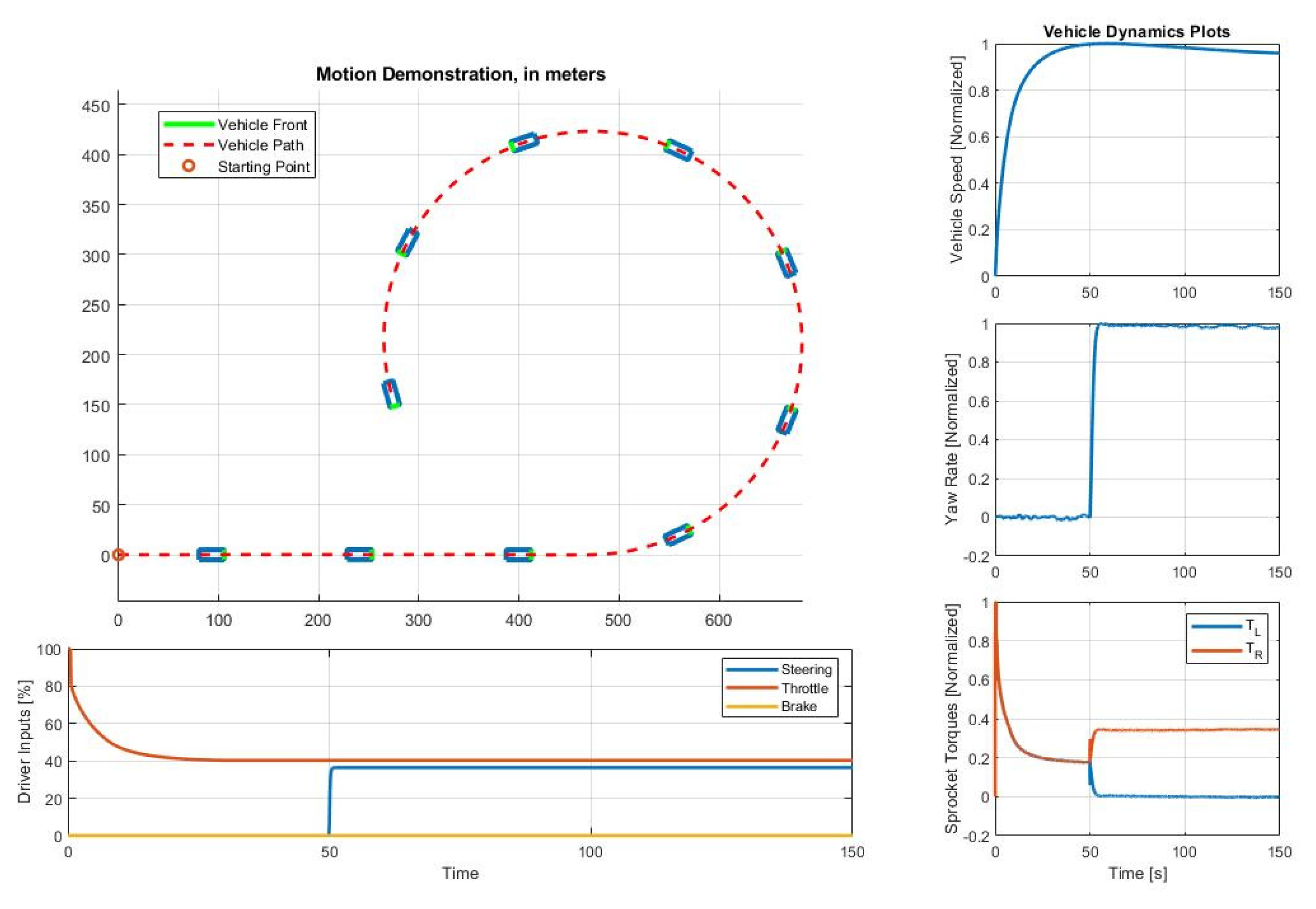
Figure 13.
Speed Differential During Cornering
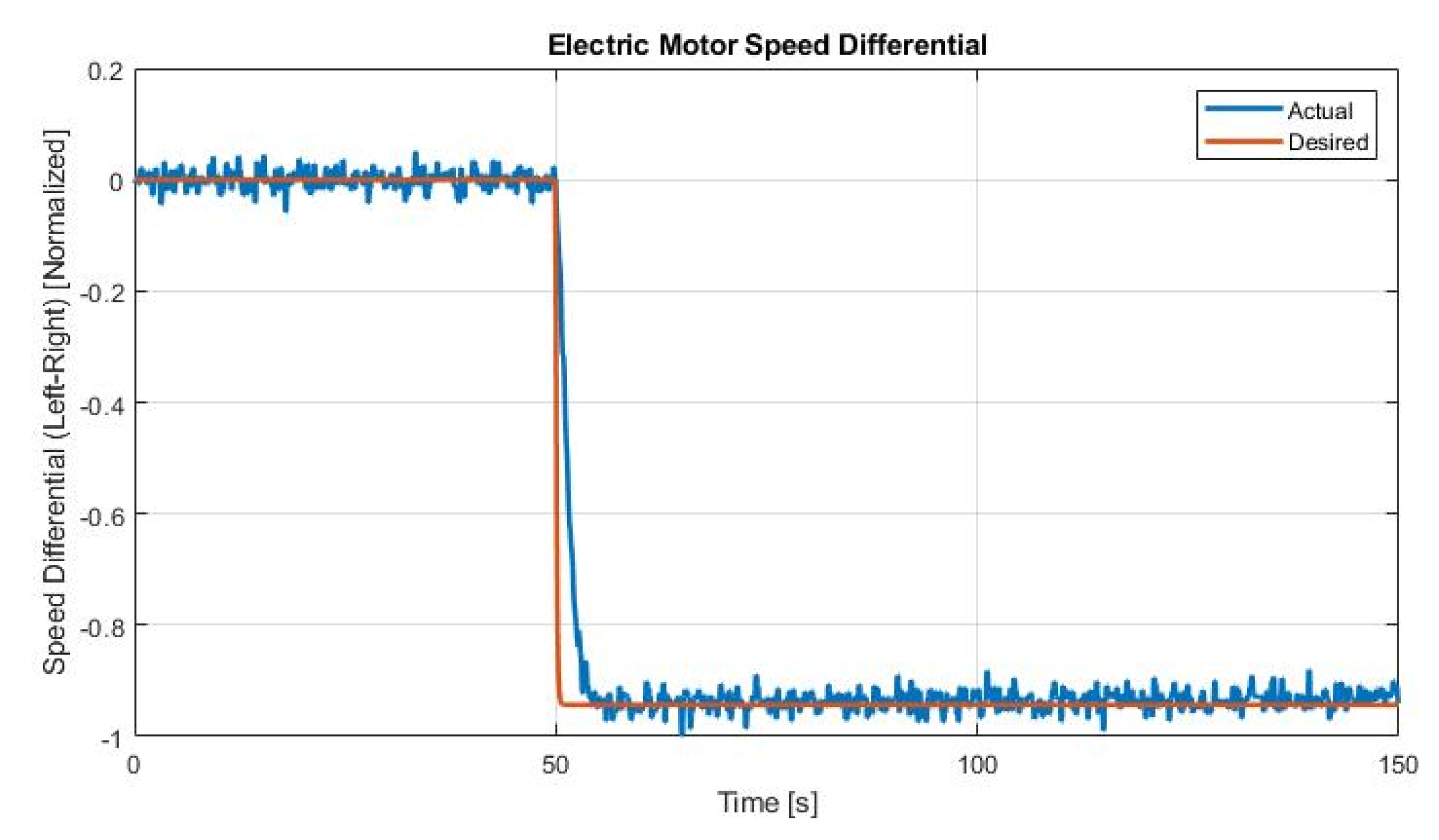
Figure 14.
Total Traction Torque of the Vehicle in Response to Accelerator Pedal Position
Disclaimer/Publisher’s Note: The statements, opinions and data contained in all publications are solely those of the individual author(s) and contributor(s) and not of MDPI and/or the editor(s). MDPI and/or the editor(s) disclaim responsibility for any injury to people or property resulting from any ideas, methods, instructions or products referred to in the content. |
© 2024 by the authors. Licensee MDPI, Basel, Switzerland. This article is an open access article distributed under the terms and conditions of the Creative Commons Attribution (CC BY) license (http://creativecommons.org/licenses/by/4.0/).
Copyright: This open access article is published under a Creative Commons CC BY 4.0 license, which permit the free download, distribution, and reuse, provided that the author and preprint are cited in any reuse.


