Research on Strain Transfer Study of FBG Strain Sensor Attached on a Novel Pipe Material (ABR) under Static and Dynamic Load with Calibration Test

The metrological performance of FBG strain sensing systems is a critical premise for the precision of plastics water support pipeline structural deformation measurement, but the strain transfer loss of FBG attached on the plastics pipe subjected by dynamic force is unclear. This paper presents the first study on the effects of strain transfer between FBG, and acrylate polymer blended with poly resin (ABR)pipe sheets loaded by static and dynamic force. Theoretical methods of dynamic strain transfer theory combine with the exponentially decaying sinusoidal shock force time course is deduced and various dynamic parameters sensitivities studies are carried out, as well as that of the geometric parameters. The result of the dynamic theory is compared with the calibration test outcomes, while the ASTR of FBG attached on ABR sheet is compared with distributed optical fiber sensors (DOFS) and other pipe materials such as PVC, concrete, and steel. Results show that the ASTR of FBG is more accurate than that of the DOFS, and the grows of ASTR depending on the paste length of FBG, the Young's modulus of the middle materials, the thickness of the middle materials and attenuation coefficient. Paste length produced the largest increase, yet the magnitude and loading speed of the external force has unexpectedly little effect on ASTR. FBG seem low error, insensitive with dynamic force and independent with the material of matrix, and this demonstrates benefits that are stronger across the board than DOFS. This is not currently recognized by standards or by most reported studies.

Keywords:

Subject:

Engineering - Civil Engineering

1. Introduction

The health status of plastic water conveyance pipelines exerts a substantial influence on economic development, transportation, and societal well-being[1,2]. Vigilant monitoring of plastic water pipelines is imperative, particularly in the context of strain surveillance within the pipeline framework. Cutting-edge, expansive distributed intelligent sensing components, exemplified by Fiber Bragg Grating (FBG) sensors, lay the groundwork for the evolution of health monitoring systems for pipeline structures[3,4]. FBG strain sensors, characterized by robust immunity to electromagnetic interference, elevated precision, commendable longevity, and the capacity for distributed measurement, are instrumental in this regard. During the health monitoring of pipelines, optical fiber strain sensors are typically operated within dynamic scenarios[5]. Any inaccuracies in the measurement data of these sensors may introduce adverse effects on subsequent control, monitoring, and fault diagnostic systems, potentially resulting in detrimental occurrences such as misdiagnoses and false alarms, with significant repercussions. Therefore, it becomes imperative to subject FBG strain sensors utilized in practical scenarios to calibration processes to ensure the precision of measurement outcomes.

The main challenge faced by many researchers is the accuracy of FBG compared with the traditional sensing technology such strain gauges. Recently investigators have examined the effects of strain transfer on the optical fiber sensors. Fiber optic sensors are composed of a fiber core and a sheath, which can be affixed to the structure's surface by adhesive, buried within the structure, or secured to the structure by mechanical devices. Regardless of the method chosen, the actual strain of the structure to be measured is inevitably subjected to losses as it passes through the adhesive, sheath, and other intermediate media to reach the core part of the fiber optic sensor. Consequently, a certain gap exists between the strain measured by the fiber optic core and the actual deformation of the structure, giving rise to what is known as the strain transfer loss phenomenon. The strain loss resulting from this transfer is termed the rate of strain transfer, and the strain transfer loss constitutes one of the primary sources of measurement error in optical fiber.

The utilization of the strain transfer theory to calculate the optical fiber strain transfer rate has been proposed by researchers[6] to eliminate the measurement error of optical fibers. The strain transfer theory, originally introduced by Cox[7], focuses on investigating the collaborative deformation of adjacent materials under external forces and was initially applied to analyze thread breakage and drawing behavior in textiles. Subsequently, enhancements to the strain transfer theory were made by Eshelby[8], who adapted the theory to meet the specific requirements of physics and engineering. They employed the dissection-deformation-combination analytical method to scrutinize the forces acting on composites wrapped with different geometries of built-ups, exploring the impact of material inhomogeneity in wrapped bodies and elliptical built-ups on their overall deformation field. Furthermore, Rosen[9], CHOON[10], and others utilized the strain transfer theory to analyze the shear hysteresis phenomenon occurring at the material contact surface due to the unilateral stressing of composites. As a result, strain transfer theory is also recognized as shear lag theory.

One major theoretical issue that has dominated the field for many years concerns is the parameter sensitive of strain loss. The effect of paster method on strain transfer loss is studies by Nanni[11], Duck[12], Dasgupta[13], contains external and embedded layout. The influence of layers on strain transfer loss is examined by Yuan[14], Ansari[15], Lau[16], LeBlanc[17], Her[18,19], involving two, three, four layers, respectively. The design of fiber armed is investigated by Torres[20], Li[21,22], Billon[23], Luyckx[24], addressing its impact on strain transfer loss and encompassing naked fiber, PVC armed, mini pipe, mental armed. Strain transfer loss is analyzed concerning the service circumstance, with contributions from Wang[25,26,27], Liu[28,29,30], Ansari[31] who highlighting in uneven matrix, fatigue load, distribution of external forces.

Such approaches, however, have failed to address the strain transfer loss of FBG subjected by dynamic loads. Firstly, much of the research up to now has been descriptive and theoretical, which is lack validation by experimental data. Secondly, researchers have not treated dynamic loading in much detail, which is not treated as a background in the analysis. Thirdly, although extensive research has been carried out on strain transfer loss, no single study exists which paste methods is suitable for pipe deformation measurement. Lastly, previous analysis does not take account of the difference of FBG attached on various pipe materials, nor does the examination of strain sensing technology such as FBG, OFTR and BOTDA. With such shortage, it is not clear whether the measured result of FBG attached on ABR pipe and other water support pipe is believable or not.

In conclusion, the foregoing discussion has underscored the significance of strain transfer ratio of FBG. The identified gaps in the current understanding of strain transfer loss highlight the need for further investigation. The primary objective of this study is to study the strain transfer of FBG attached on a novel pipe material (ABR) under static and dynamic load with calibration test, shedding light on the strain loss relate to the dynamic force. A three-layer dynamic strain transfer theory for the calculation of STR and ASTR of FBG subjected by dynamic loading is deduced, and the parameter sensitive is analyzed. The calibration test for ABR-measurement FBG is designed, and the test results of ASTR is compared with the theoretical outcome. The experimental and theoretical work presented here provides one of the first investigations into how to analysis the strain transfer loss of FBG attached on ABR pipe, which will be used on a large scale in the project.

2. Strain Transfer of FBG under Dynamic Excitation

2.1. Static FBG strain transfer theory and dynamic one

2.1.1. Static strain transfer theory of FBG

The strain transfer theory which proposed by Ansari[15] and Song[21] can be used to analyze the relationship between the actual strain of the structure and the strain of the fiber optic sensor. The assumptions of the theoretical model are given: (1) All materials are recognized as elastic. (2) Axial stress is attached on the matrix solely. (3) The mechanical properties of the cladding and the fiber optic core are the same, which are collectively known as optical fiber sensors. (4) There is no debonding phenomenon at all interfaces. The mechanical model of the theory is shown in Figure 1.

Where r_f is the radius of the optical fibers, r_p is the radius of the middle layer; σ_f is the stress of the optical fibers, σ_p is the stress of the middle layer, σ_m is the stress of the matrix; τ_fp is the shear stress on the surface of middle layer and optical fibers, τ_pm is the shear stress on the surface of middle layer and matrix. As is deduced in Song’s literature, the strain attenuation formula is shown in Eq.1~2.

ε_{f} (x, r_{f}) = ε_{m} (x, r_{p}) [1 - \frac{\cosh (λ x)}{\cosh (λ L)}]

(1)

λ^{2} = \frac{2 G_{p}}{E_{f} r_{f}^{2} \ln (\frac{r_{p}}{r_{f}})}

(2)

Where λ is the shear-lag parameter, L is the paste length, G_p is the shear modulus of the middle layer, E_f is the Young's modulus of the optical fibers, ε_f is the strain of the optical fibers, ε_m is the strain of the matrix. Furthermore, the strain transfer ratio (STR) and the average strain transfer ratio (ASTR) of optical fiber sensors is shown in Eq.3 and Eq.4.

STR = 1 - \frac{\cosh (λ x)}{\cosh (λ L)}

(3)

ASTR = \frac{\bar{ε_{f} (x, r_{f})}}{ε_{m} (x, r_{p})} = \frac{2 \int_{0}^{L} ε_{f} (x, r_{f}) d x}{2 L ε_{m} (x, r_{p})} = 1 - \frac{\sinh (λ L)}{λ L \cosh (λ L)}

(4)

2.1.2. Dynamic strain transfer theory of FBG

The four layer dynamic strain transfer theory contains the“core-coat-adhesive-matrix” structure deduced by Wang[25] can be used for the deformation monitoring of structures which are subjected by vibration, alternating and shock loads. Moreover, a three layer dynamic strain transfer theory contain the“core-middle-matrix” structure is deduced in this section. Compared with the static theory, one additional assumption is declared, that is said the damping of these materials should be ignored. Same as the Figure 1, but the force balance of each part exhibits a bit different. The force balance of optical fiber sensors is shown in Figure 2, and the corresponding equations are proposed in Eq.5：

\begin{array}{l} \sum F_{f} = P_{f} \\ π r_{f}^{2} d σ_{f} + 2 π r_{f} d x τ_{fp} (x, r_{f}) = ρ_{f} π r_{f}^{2} d x \frac{\partial^{2} u_{f}}{\partial t^{2}} \end{array}

(5)

Where dx is the length of infinitesimal body,

\sum F_{f}

is the sum of the force of the optical fibers on the x-axis, P_f is the inertial force of the optical fibers, ρ_f is the density of the optical fibers. Furthermore, The force balance of the middle layer is shown in Figure 3, and the corresponding equations are proposed in Eq.6：

\begin{array}{l} \sum F_{p} = P_{p} \\ (π r_{p}^{2} - π r_{f}^{2}) d σ_{p} + 2 π r_{p} d x τ_{pm} (x, r_{p}) - 2 π r_{f} d x τ_{fp} (x, r_{f}) = ρ_{p} (π r_{p}^{2} - π r_{f}^{2}) d x \frac{\partial^{2} u_{p}}{\partial t^{2}} \end{array}

(6)

Where

\sum F_{p}

is the sum of the force of middle layer on the x-axis, P_p is the inertial force of the middle layer, ρ_p is the density of the middle layer. The expressions of the shear stress can be transferred by Eq.6, gives：

τ_{pm} (x, r_{p}) = \frac{ρ_{p} (r_{p}^{2} - r_{f}^{2})}{2 r_{p}} \frac{\partial^{2} u_{p}}{\partial t^{2}} + \frac{ρ_{f} r_{f}^{2}}{2 r_{p}} \frac{\partial^{2} u_{f}}{\partial t^{2}} - \frac{r_{f}^{2}}{2 r_{p}} \frac{d σ_{f}}{d x} - \frac{(r_{p}^{2} - r_{f}^{2})}{2 r_{p}} \frac{d σ_{p}}{d x}

(7)

τ (x, r) = \frac{ρ_{p} (r^{2} - r_{f}^{2})}{2 r} \frac{\partial^{2} u_{p}}{\partial t^{2}} + \frac{ρ_{f} r_{f}^{2}}{2 r} \frac{\partial^{2} u_{f}}{\partial t^{2}} - \frac{r_{f}^{2}}{2 r} \frac{d σ_{f}}{d x} - \frac{(r^{2} - r_{f}^{2})}{2 r} \frac{d σ_{p}}{d x}

(8)

The Poisson effect of FBG can be ignored by the consideration of lager L/D ratio. Then, the strain gradient and the acceleration of each layer is assumed as the same, gives：

\frac{\partial^{2} u_{f}}{\partial t^{2}} \approx \frac{\partial^{2} u_{p}}{\partial t^{2}}, \frac{d ε_{f}}{d x} \approx \frac{d ε_{p}}{d x}

(9)

Eq.8 can be transferred as follows:

τ (x, r) = [\frac{ρ_{p} (r^{2} - r_{f}^{2})}{2 r} + \frac{ρ_{f} r_{f}^{2}}{2 r}] \frac{\partial^{2} u_{p}}{\partial t^{2}} - [\frac{r_{f}^{2} E_{f}}{2 r} + \frac{(r^{2} - r_{f}^{2}) E_{p}}{2 r}] \frac{d ε_{f}}{d x}

(10)

Eq.11 is given based on materials mechanics：

τ = G \frac{d u}{d r}

(11)

Then, Eq.11 is subjected to Eq.10, and integrating r once on the equation：

\int_{r_{f}}^{r_{p}} G_{p} \frac{d u}{d r} d r = \int_{r_{f}}^{r_{p}} [\frac{ρ_{p} (r^{2} - r_{f}^{2})}{2 r} + \frac{ρ_{f} r_{f}^{2}}{2 r}] \frac{\partial^{2} u_{p}}{\partial t^{2}} d r - \int_{r_{f}}^{r_{p}} [\frac{r_{f}^{2} E_{f}}{2 r} + \frac{(r^{2} - r_{f}^{2}) E_{p}}{2 r}] \frac{d ε_{f}}{d x} d r

(12)

Eq.12 is organized and gives:

G_{p} \int_{r_{f}}^{r_{p}} \frac{d u}{d r} d r = \frac{\partial^{2} u_{p}}{\partial t^{2}} \int_{r_{f}}^{r_{p}} [\frac{r}{2} ρ_{p} + \frac{r_{f}^{2}}{2 r} (ρ_{f} - ρ_{p})] d r - \frac{d ε_{f}}{d x} \int_{r_{f}}^{r_{p}} [\frac{r}{2} E_{p} + \frac{r_{f}^{2}}{2 r} (E_{f} - E_{p})] d r

(13)

u_{p} - u_{f} = \frac{\partial^{2} u_{p}}{\partial t^{2}} [\frac{r_{p}^{2} - r_{f}^{2}}{4 G_{p}} ρ_{p} + \frac{r_{f}^{2}}{2 G_{p}} \ln \frac{r_{p}}{r_{f}} (ρ_{f} - ρ_{p})] - \frac{d ε_{f}}{d x} [\frac{r_{p}^{2} - r_{f}^{2}}{4 G_{p}} E_{p} + \frac{r_{f}^{2}}{2 G_{p}} \ln \frac{r_{p}}{r_{f}} (E_{f} - E_{p})]

(14a)

u_{p} - u_{f} = - \frac{1}{λ_{D}^{2}} \frac{d ε_{f}}{d x} + Δ \frac{\partial^{2} u_{p}}{\partial t^{2}}

(14b)

Thus, the equation of solution for the strain of optical fiber is given:

\frac{d^{2} ε_{f}}{d x^{2}} - λ_{D}^{2} ε_{f} + λ_{D}^{2} [ε_{p} - Δ \frac{\partial}{\partial x} (\frac{\partial^{2} u_{p}}{\partial t^{2}})] = 0

(15)

Δ = \frac{r_{p}^{2} - r_{f}^{2}}{4 G_{p}} ρ_{p} + \frac{r_{f}^{2}}{2 G_{p}} \ln \frac{r_{p}}{r_{f}} (ρ_{f} - ρ_{p})

(16)

\frac{1}{λ_{D}^{2}} = \frac{r_{p}^{2} - r_{f}^{2}}{4 G_{p}} E_{p} + \frac{r_{f}^{2}}{2 G_{p}} \ln \frac{r_{p}}{r_{f}} (E_{f} - E_{p})

(17)

Where λ_D is the shear-lag parameter subjected by the dynamic load，Δ is the parameter relates to the density of optical fiber and middle layer.

In this section, an exponentially decaying sinusoidal shock force time course is used as an example：

F (t) = A \cdot e^{- B t} \cdot \sin (2 π f t)

(18)

Where F(t) is the impact force on the matrix, A is the amplification, B is the attenuation coefficient, f is the frequency. The relationships of velocity and acceleration is given in Eq.19 by Newton's second law.

\frac{\partial^{2} u_{m}}{\partial t^{2}} = \frac{\partial^{2} u_{m}}{\partial x^{2}} \cdot \frac{\partial x^{2}}{\partial t^{2}} = \frac{\partial^{2} u_{m}}{\partial x^{2}} \cdot {(\frac{\partial x}{\partial t})}^{2} = \frac{\partial^{2} u_{m}}{\partial x^{2}} \cdot {[v_{m} (x, t)]}^{2}

(19)

Where v_m(x,t) is velocity of matrix, the elastic wave velocity equation for solids is given:

v_{m} (x, t) = \sqrt{\frac{E_{m}}{ρ_{m}}}

(20)

Where ρ_m is the density of the matrix, E_m is the Young's modulus of the matrix, Eq.20 is transferred as follows:

\frac{\partial^{2} u_{m}}{\partial t^{2}} = \frac{\partial^{2} u_{m}}{\partial x^{2}} \cdot \frac{E_{m}}{ρ_{m}}

(21)

The relationship of the impact force F(t) and the deformation of matrix ε_m(0,t) is given:

E_{m} \cdot S_{m} \cdot ε_{m} (0, t) = F (t) = A \cdot e^{- B t} \cdot \sin (2 π f t)

(22)

Where S_m is the cross-section area of the matrix, and the displacement of the matrix is given：

{\frac{\partial u_{m}}{\partial x} |}_{x = 0} = \frac{A}{E_{m} \cdot S_{m}} \cdot e^{- B t} \cdot \sin (2 π f t)

(23)

And the perpendicular displacement of the matrix is given based on the symmetry assumption:

u_{m} (0, t) = 0

(24)

The steady-state response of the matrix based on Eq.22~ Eq.24 is solved by the split-variable method：

u_{m} (x, t) = \bar{U} (x) \cdot e^{- B t} \cdot \sin (2 π f t)

(25)

Where

\bar{U} (x)

is a part of the expression which only contains variable x, and the boundary condition of

\bar{U} (x)

\bar{U} (0) = 0

(26)

{\frac{\partial \bar{U} (x)}{\partial x} |}_{x = 0} = \frac{A}{E_{m} \cdot S_{m}}

(27)

The form of

\bar{U} (x)

is configured as:

\bar{U} (x) = C_{1} x + C_{2}

(28)

Where C₁ and C₂ is the parameters which is solved by Eq.26~ Eq.27:

\bar{U} (0) = C_{2} = 0

(29)

{\frac{\partial \bar{U} (x)}{\partial x} |}_{x = 0} = \frac{A}{E_{m} \cdot S_{m}} = C_{1}

(30)

Then the steady-state response of the matrix is given：

u_{m} (x, t) = \frac{A}{E_{m} \cdot S_{m}} x \cdot e^{- B t} \cdot \sin (2 π f t)

(31)

ε_{m} (x, t) = \frac{A}{E_{m} \cdot S_{m}} \cdot e^{- B t} \cdot \sin (2 π f t)

(32)

The first order derivative of t in Eq.31 is token, and the velocity of the substrate is given as follows:

v_{m} (x, t) = \frac{- A \cdot B}{E_{m} \cdot S_{m}} x \cdot e^{- B t} \cdot \sin (2 π f t) + \frac{2 π A \cdot f}{E_{m} \cdot S_{m}} x \cdot e^{- B t} \cdot \cos (2 π f t)

(33)

The first order derivative of t in Eq.33 is token, and the acceleration of the substrate is given as follows:

\begin{array}{l} \frac{\partial^{2} u_{m}}{\partial t^{2}} = \frac{A \cdot B^{2}}{E_{m} \cdot S_{m}} x \cdot e^{- B t} \cdot \sin (2 π f t) - \frac{2 π A \cdot B \cdot f}{E_{m} \cdot S_{m}} x \cdot e^{- B t} \cdot \cos (2 π f t) \\ - \frac{2 π A \cdot B \cdot f}{E_{m} \cdot S_{m}} x \cdot e^{- B t} \cdot \cos (2 π f t) - \frac{4 π^{2} A \cdot f^{2}}{E_{m} \cdot S_{m}} x \cdot e^{- B t} \cdot \sin (2 π f t) \end{array}

(34)

The first order derivative of x in Eq.34 is token, and the expression f(t) without the various x is given as follows:

\begin{array}{l} \frac{\partial}{\partial x} (\frac{\partial^{2} u_{m}}{\partial t^{2}}) = \frac{A \cdot B^{2}}{E_{m} \cdot S_{m}} \cdot e^{- B t} \cdot \sin (2 π f t) - \frac{2 π A \cdot B \cdot f}{E_{m} \cdot S_{m}} \cdot e^{- B t} \cdot \cos (2 π f t) \\ - \frac{2 π A \cdot B \cdot f}{E_{m} \cdot S_{m}} \cdot e^{- B t} \cdot \cos (2 π f t) - \frac{4 π^{2} A \cdot f^{2}}{E_{m} \cdot S_{m}} \cdot e^{- B t} \cdot \sin (2 π f t) = f (t) \end{array}

(35)

Eq.35 is subjected into Eq.15, gives:

ε_{f} (x, r_{f}) = c_{1} e^{λ_{D} x} + c_{2} e^{- λ_{D} x} + ε_{m} - Δ \cdot f (t)

(36)

The boundary condition is proposed by recognizes that the strain on the end of the optical fiber is 0, gives:

ε_{f} (L, r_{f}) = ε_{f} (- L, r_{f}) = 0

(37)

Then the parameter of Eq.36 is solved：

c_{1} = c_{2} = - \frac{[ε_{m} - Δ \cdot f (t)]}{e^{λ_{D} L} + e^{- λ_{D} L}}

(38)

At last, gives:

ε_{f} (x, r_{f}) = - \frac{[ε_{m} - Δ \cdot f (t)]}{e^{λ_{D} L} + e^{- λ_{D} L}} (e^{λ_{D} x} + e^{- λ_{D} x}) + ε_{m} - Δ \cdot f (t)

(39)

Furthermore, the strain transfer ratio (STR) and the average strain transfer ratio (ASTR) of optical fiber sensors is shown in Eq.40~Eq.44.

STR = \frac{ε_{f} (x, r_{f})}{ε_{m} (x, t)} = - \frac{g (t)}{e^{λ_{D} L} + e^{- λ_{D} L}} (e^{λ_{D} x} + e^{- λ_{D} x}) + g (t)

(40)

g (t) = 1 - \frac{Δ \cdot f (t) E_{m} \cdot S_{m}}{A \cdot e^{- B t} \cdot \sin (2 π f t)}

λ_{D} = \frac{1}{\sqrt{\frac{r_{p}^{2} - r_{f}^{2}}{4 G_{p}} E_{p} + \frac{r_{f}^{2}}{2 G_{p}} \ln \frac{r_{p}}{r_{f}} (E_{f} - E_{p})}}

(41)

f (t) = \frac{A \cdot B^{2}}{E_{m} \cdot S_{m}} \cdot e^{- B t} \cdot \sin (2 π f t) - \frac{4 π A \cdot B \cdot f}{E_{m} \cdot S_{m}} \cdot e^{- B t} \cdot \cos (2 π f t) - \frac{4 π^{2} A \cdot f^{2}}{E_{m} \cdot S_{m}} \cdot e^{- B t} \cdot \sin (2 π f t)

(42)

Δ = \frac{r_{p}^{2} - r_{f}^{2}}{4 G_{p}} ρ_{p} + \frac{r_{f}^{2}}{2 G_{p}} \ln \frac{r_{p}}{r_{f}} (ρ_{f} - ρ_{p})

(43)

\begin{array}{l} ASTR = \frac{\bar{ε_{f} (x, r_{f})}}{ε_{m} (x, r_{p})} = \frac{2 \int_{0}^{L} {- \frac{[ε_{m} - Δ \cdot f (t)]}{e^{λ_{D} L} + e^{- λ_{D} L}} (e^{λ_{D} x} + e^{- λ_{D} x}) + ε_{m} - Δ \cdot f (t)} d x}{2 L \frac{A}{E_{m} \cdot S_{m}} \cdot e^{- B t} \cdot \sin (2 π f t)} \\ = 1 - \frac{Δ \cdot f (t)}{\frac{A}{E_{m} \cdot S_{m}} \cdot e^{- B t} \cdot \sin (2 π f t)} - \frac{[\frac{A}{E_{m} \cdot S_{m}} \cdot e^{- B t} \cdot \sin (2 π f t) - Δ \cdot f (t)] (e^{λ_{D} L} - e^{- λ_{D} L})}{λ_{D} (e^{λ_{D} L} + e^{- λ_{D} L}) \frac{A}{E_{m} \cdot S_{m}} \cdot e^{- B t} \cdot \sin (2 π f t) \cdot L} \end{array}

(44)

2.2. Comparison of the calculated results of static FBG strain transfer and dynamic one

2.2.1. Parameters for calculation

The calculation results of static theory and dynamic one is carried out by using the material parameters and dynamic parameters in Table 1 and Table 2, respectively.

2.2.2. Discuss the effect of parameters on FBG subjected by dynamic load

The results of Eq.40~Eq.44 show that the STR and ASTR of FBG is sensitive with the paste length, E_p, r_p and B. The curve of STR and ASTR shown in Figure 4 revealed that the STR is increasing with the grows of paste length, as well as the ASTR. Prior studies that have noted the importance of paste length of FBG subjected to static force, which shows a same trend with that of the dynamic ones. It should notice that the FBG should be pasted with the length of 0.06m at least for ensure the measurement accuracy of 90%. Moreover, the strain attenuation of FBG is reduced to 1% when the paste length is longer than 0.3m, as well as the DOFS.

As shown in Figure 5, one interesting finding is that the STR and ASTR of FBG shows a decrease trend with the grows of E_p. These findings are somewhat surprising given the fact that other research shows an exactly opposite results to that of the trend under static loads. Leblanc et al. (1998) showed that the higher the E_p, the higher the STR and ASTR. Since this difference has not been found elsewhere it is probably not due to the traditional explanation that the shear deformation of middle layer is decrease with the grows of E_p. This discrepancy could be attributed to the deformation of middle layer is increased with the decline of E_p. In that case, a part of the strain attenuation of FBG has been complemented by the dynamic deformation middle layer due to the inertial force. Further, the results of the study show that the E_p should not exceed 1.2GPa.

It is interesting to compare Figure 6 with Figure 4 and Figure 5 in Yuan[32] that shows a similar result of the trend with r_p and STR, where the grows of STR has been found smaller than that in this study. It should be noticed that this finding is recognized based on the same parameter used in Ansari[15] and this study. It seems possible that these results are due to the r_p is a more sensitive parameter in dynamic analysis than that of in static ones. Therefore, the r_p thicker than 5mm is not suggested.

The most important finding is that the curve of STR and ASTR exhibits a close relates with the attenuation coefficient B, but nearly not affected by the changes in A, f, E_m, S_m, t. Various data of A, f, E_m, S_m, t are submitted into Eq.40~Eq.44 and no clear trend has been found.

The above findings of FBG strain transfer affected by dynamic parameters are positive. These results indicates that STR and ASTR is insensitive with the A, f, E_m, S_m, t. In that case, FBG can be applied on the matrix with unlimited range of volumes, various material performances, subjected by any amplitude or velocity of external forces. In that case, the strain attenuation of the matrix strain measured by FBG can be used after modified by FBG geometry only.

3. Calibration test

3.1. Test set up

3.1.1. Fabrication of calibration device

As is shown in Figure 8, a designed device for static and dynamic calibration of FBG is proposed. The novelty of this device is recognized that the sheet of matrix can be exchanged to other sheet that made of different pipe materials. That is, the strain transfer ratio of FBG on various pipe materials can be calibrated. The main structure of this device is based on the basic operation of optical fiber sensor calibration test. It should be mentioned that the size of the sheet of matrix is designed by using the equal-strength cantilever beam theory, which is introduced in section 3.2.2. the other part of the device is made of steel.

3.1.2. Methods of the test

The test can be divided into static test and dynamic test, as is shown in Figure 9 and Figure 10, respectively. In the static test, the strain of the FBG is calibrated by the strain gauge. The strain of the DOFS is arranged as an additional initiative for sensors calibration and a modification for the consistency of the surface strain on the sheet. The static calibrate test should be developed as follows: (1) FBG, Strain gauge and DOFS is attached on the sheet; (2) The sheet is retained on the device; (3) The weights is put onto the hook, and it should be adapted by observes the data of DOFS until the strain on the surface of the sheet is equals everywhere; (4) The data of FBG and strain gauges is collected; (5) The weights is put off from the hook and then put back, the data of FBG and strain gauges is recollected; (6) This test is repeated four times.

In the dynamic test, the strain of the FBG is also calibrated by the strain gauge. The strain of the DOFS is arranged as an additional initiative for sensors calibration and a modification for the consistency of the surface strain on the sheet. Additionally, the acceleration sensors are arranged for the dynamic force calculation. The dynamic calibrate test should be developed as follows: (1) FBG, Strain gauge, acceleration sensors and DOFS is attached on the sheet; (2) The sheet is retained on the device; (3) The weights is put onto the top of the hook, and then the weights drop from the top and on to the bottom of the hook; (4) The data of FBG and strain gauges is collected; (5) The weights is put back to the top of the hook and then fall again, the data of FBG and strain gauges is recollected; (6) This test is repeated four times.

3.1.3. Methods of the pretest

In the stage of the pretest, the initial value of strain gauge and FBG is recorded by the FBG demodulator and Dynamic Signal Collector. This initial value measurement time T₁ is 3s. Then, a weight has been installed on the device and the static value of strain gauge and FBG is also stored. This static value measurement time T₂ is 3s, but the stable time after the weight install is 10s.The above experimental process is repeated for three times to obtain the corresponding data. It should be noticed that the ambient temperature should be keep constant at 20°C, while the laboratory is basically free from ambient vibration and noise. The specimen S-1 is proposed for this pretest.

3.2. Fabrication of specimens

3.2.1. Details of the grouping information

In this test, four materials are used to make the sheet, including steel, concrete, PVC, and ABR. ABR is the acrylate polymer blended with poly resin which is used for a novel water support pipeline. The grouping information is exhibited in Table 2. There are three specimens of each material are manufactured. The different of each specimen is that the paste method, including Type A, Type B and Type C. It should be notice that the sheet of the ABR is cut from the real pipe, and the details of the ABR pipe is introduced in Shan’s report[33]. The PVC and steel sheet is made by molds, and the concrete sheet has being poured for months.

Table 2. Material parameters of FBG sensors in this paper for theory.

Num of specimens	Materials	Paste	sensors
S-1	Steel	Type A	Strain gauge, FBG, DOFS
S-2	Steel	Type B	Strain gauge, FBG, DOFS
S-3	Steel	Type C	Strain gauge, FBG, DOFS
C-1	Concrete	Type A	Strain gauge, FBG, DOFS
C-2	Concrete	Type B	Strain gauge, FBG, DOFS
C-3	Concrete	Type C	Strain gauge, FBG, DOFS
P-1	PVC	Type A	Strain gauge, FBG, DOFS
P-2	PVC	Type B	Strain gauge, FBG, DOFS
P-3	PVC	Type C	Strain gauge, FBG, DOFS
A-1	ABR	Type A	Strain gauge, FBG, DOFS
A-2	ABR	Type B	Strain gauge, FBG, DOFS
A-3	ABR	Type C	Strain gauge, FBG, DOFS

3.2.2. Sheet of matrix setup

The geometric parameters of sheet are shown in Figure 12. The width of the short side b has been per-set as 5mm, and the length of the purely curved segment t′ is 30cm. These two coefficients are based on the reported study. Based on basic knowledge of equal strength cantilever beam, the angle of the sheet is calculated by Eq.45. Where G is the weights and G=5kg, h is the thicknesses of the sheet. t-t′ is one part of the sheet for hanging the weights, B is the width of the long side of the sheet.

\tan α = \frac{3 G}{σ h^{2}}

(45)

Table 3. Dimensions of the specimen.

Materials	B	b	t′	t	L	h
Steel	9cm	5mm	30cm	40cm	50cm	1mm
Concrete		5mm	30cm	40cm	50cm	20mm
PVC	7cm	5mm	30cm	40cm	50cm	13mm
ABR	7cm	5mm	30cm	40cm	50cm	13mm

3.2.3. Sensors and layout

The Distributed optical fiber sensors (DOFS) and Fiber Bragg Grating sensors (FBGs) is used in this test, as shown in Figure 13. The paste methods, which are mentioned in section 3.2.1, are introduced in Figure 14. There are three types of paste method are proposed in this test: Type A is the all-inclusive rectangular paste method; Type B is the half-inclusive rectangular paste method; Type C is the normal paste method which is the most widely used. The paste method of optical fiber sensors should be compared, for the geometry of adhesive is one of the most sensitive parameters of STR and ASTR. Specifically, the shortage of Type C is recognized that the cross-section of Type C is hard to be maintained. Hence it should be compared with Type A. However, the effect of cover layer of Type A on strain transfer should be studied. In that case, Type B is carried out.

As is shown in Figure 15, DOFS is pasted alone the sheet, where FBG and Strain gauge are pasted on the middle of the sheet. it should be mentioned that the paste method of DOFS and FBG are the same. The sensed specimens are shown in Figure 16. the paste length of FBG is 6cm and the DOFS is 30cm.

3.3. Performance of the equipment and sensing technology

3.3.1. FBG demodulator

The experimental study in this paper using FBG is conducted using the Zx-fg-c04-100 fiber grating demodulator produced by Wisdom Technology Nantong Co., which is commonly employed in experimental setups in the field of scientific research. This device is shown in Figure 17.

The demodulator is equipped with four channels, each of which can be serially connected to 4~8 fiber grating sensors. A sampling frequency of 100Hz is employed, and the specific performance parameters are detailed in Table 1.

Table 4. Performance of fiber grating demodulator（Type Zx-fg-c04-100）.

Parameter	Units	Details
Number of channels	CH	4
Number of sensors per channel	PCS	temperature：8；strain：4
Monitoring wavelength range	nm	1530-1550
Sampling frequency	Hz	100
Strain sensitivity coefficient	nm/με	0.000716
Temperature sensitivity coefficient	nm/℃	0.016498
Equipment working humidity	%	0-75

Tips: Data sourced from Zhixing Technology Nantong Co., Ltd

The relationship between wavelength, strain and temperature for fiber grating sensors is depicted in Eq.46.

λ_{B} = 2 n Λ = Δ ε \cdot α_{ε} + Δ T \cdot α_{T}

(46)

Where a_ε and a_T is the strain and temperature coefficients of FBGs, respectively; λ_B is the wavelength of FBGs, n is the refractive index of FBGs, Λ is the period of FBGs, Δε is the strain variation, ΔT is the temperature variation.

3.3.2. BOTDA demodulator

The experimental study in this paper using DOFS is conducted using the DITEST STA-R Series demodulator produced by Omnisens, which is based on Brillouin Optical Time Domain Analysis (BOTDA) technology. This device is shown in Figure 18.

Two channels are set on the device, where the resolution of monitoring is 10cm，the performance of distributed fiber optic demodulator is shown in Table 2.

Table 5. Performance of distributed fiber optic demodulator（Type DITEST STA-R Series）.

Parameter	Units	Details
Channel		2
Distance	km	50
Distance resolution	m	0.1
Range of Strain		-3%~3%
Measurement time	min	1~2

Tips: Data sourced from Beijing Tongwei Science & Technology Co.

The relationship between Brillouin frequency shift, strain and temperature for fiber grating sensors is depicted in Eq.47.

Δ v_{B} = Δ ε \cdot C_{ε} + Δ T \cdot C_{T}

(47)

Where C_ε and C_T is the strain and temperature coefficients of BOTDA signal, respectively; Δv_B is the Brillouin frequency shift variation, Δε is the strain variation, ΔT is the temperature variation.

3.3.3. OTDR demodulator

The experimental study in this paper using DOFS is conducted using the OSI-D dynamic demodulator produced by Wuhan Megasense Technologies Co., which is based on Optical Frequency Domain Reflectometry (OFDR) technology. This device is shown in Figure 19. The performance of distributed fiber optic demodulator is shown in Table 6.

The relationship between wavelength, strain and temperature is depicted in Eq.48.

Δ λ / λ = - Δ v / v = ε \cdot K_{ε} + Δ T \cdot K_{T}

(48)

Where K_ε and K_T is the strain and temperature coefficients of FBGs, respectively; λ and Δλ is the wavelength and its’ variation, Δε is the strain variation, ΔT is the temperature variation.

4. Results and Discussion

4.1. Results of the test

4.1.1. Results of the pretest

The first set of the pretest examined the cooperative of FBG, DOFS and strain gauge. Figure 20a shows the experimental data on the initial value of each sensor. What is interesting about the data in this figure is that the value of FBG and DOFS is extraordinarily similar. This finding suggests that the initial install stress of FBG and DOFS which attributed by solidification reaction of epoxy resin and the axial prestressing imposed by operator can be totally ignored. Figure 20a reveals that there has been a sharp increase in the middle of the curve of the strain gauges, which seems possible due to the electromagnetic interference (EMI).

As show in Figure 20b, there is a significant positive correlation between FBG-verified, DOFS-verified and strain gauge. After the curve of FBG has been verified by the theoretical methods reported in Eq.3 and Eq.4, the curve of FBG-verified exhibits a good relationship with that of the strain gauge, as well as the DOFS ones. This result indicates that the design of this test is feasible. Moreover, the range of the strain value indicates that the error of FBG is minimized. It should be noticed that the strain value of DOFS is the average one.

The grows of the strain distributed on the paste length of DOFS is shown in Figure 20c. What can be clearly seen in this figure is the continual growth of strain value, which agrees well with Figure 6 reported by Bao[34]. This results also suggest that the strain alone the sheet is uniform. However, the strain distribution measured by BOTDA is bad, for the resolution of BOTDA demodulator is closely to the total length of the sheet, which lead to an irregular result.

4.1.2. Results of the static test

The matrix strain measured by strain gauge is regarded as the real strain of the sheet. Hence, the ratio of FBG and strain gauge is the ASTR of FBG, where the length of the ASTR is 1cm. As is shown in Table 7 and Table 8, all the specimens have been tested by three times. On average, the steel sheet is shown to have the largest deformation, and the minimize deformation is provided by concrete sheet. The results of the sheet suggest that the most stable measured strain is the sensors attached on the concrete. A possible explanation for this might be that the concrete materials is less affected by the dynamic agitation when the weight is put on the device. That is also recognized that the study of dynamic performance of FBG measurement is needed. Another alternative explanation for this result is that it is due to the subsequent deformation of concrete sheet is virtually invisible.

The average strain of FBG, DOFS and strain gauge attached on each sheet are shown in Figure 21–Figure 23, respectively. The ASTR of FBG and DOFS with a calculation length 1cm and paste length 6cm is proposed in Figure 24. Strong evidence of the supporting of Type B is found when the ASTR of FBG and DOFS attached on steel, PVC and ABR is proved much higher than that of the others. This result suggests that the ASTR of Type B is the holistically effective one.

From this data, we can also see that static ASTR study resulted in the lowest value of concrete sheet using FBG by Type C and DOFS by Type B. It is difficult to explain this result, but it might be related to the unevenness of the surface of the concrete sheet. Type B is probably more sensitive with the surface condition of the matrix that Type A, for the adhesive thickness of Type B is the lowest one. It has been proved in Bao’s report[35] that the adhesive thickness is one of the most influential parameters of ASTR. Further, the unexpected decline is occurred due to the inhomogeneous deformation of concrete sheet result in the unevenly distributed concrete components.

Broadly, a closely relationship of ASTR between FBG and DOFS has been found. These results suggest that the measurement quality of FBG and DOFS is proven similar. However, with a small sample size, caution must be applied, as the findings might not be a strong support for whatever the FBG and DOFS is the most suitable sensors attach on various matrix. Even the lowest ASTR of DOFS is exhibited in Figure 24 (b), many positive results have been reported[1,2,36,37,38,39,40].

4.1.3. Results of the dynamic test

As is shown in Figure 25, strain of the dynamic loading on sheet S-1 is exhibited. Strain curve of sensors peaked 4 times before 0.01s, which propose a marked decline with the grows of impact time. The development of these strain curves evolves into stable in 0.02s, and the waveform matching of these sensors are relative well. This result suggests that the waveform is good for calibrations and the correlation function is not required. Additionally, as shown in Table 9, an extra evident is proposed by FBG/ DOFS which exhibits a highly compatible. A slight difference of FBG/ DOFS compare with that of the static is observed that the strain of FBG is a tiny lower that DOFS in the dynamic test.

4.2. Comparison of theoretical and experimental outcome

4.2.1. Comparison of the static result of the test

The ASTR calculated formular of Type A is introduced in Section 2.1, as shown in Eq.2~ Eq.4. An ASTR calculated formular of Type B is reported by Ye, gives:

ASTR = (1 - \frac{\sinh (λ \cdot L)}{λ \cdot \cosh (λ \cdot L) \cdot L}) \cdot \frac{1}{(1 + \frac{π \cdot E_{f} \cdot r_{f}^{2}}{a_{2} \cdot b_{1} \cdot E_{m}})}

(49)

λ^{2} = (\frac{π \cdot r_{p}}{a_{2} \cdot b_{1} \cdot E_{m}} + \frac{r_{p}}{r_{f}^{2} \cdot E_{f}}) \cdot \frac{1}{[\frac{a_{2}}{G_{a}} + \frac{r_{p}}{G_{p}} \cdot \ln (\frac{r_{p}}{r_{f}})]}

(50)

Where a₂ is thickness of the adhesive, b₁ is the width of the adhesive.

An ASTR calculated formular of Type C with the consideration of the interstice between the adhesive and the matrix is reported, gives:

ASTR = \frac{1}{E_{f} (\frac{π r_{f}^{2}}{2 h_{m} r_{p} E_{m}} + \frac{1}{E_{f}})} [1 - \frac{\sinh (λ L)}{λ L \cosh (λ L)}]

(51)

λ = \sqrt{[\frac{2 r_{p}}{π r_{f}^{2}} (\frac{π r_{f}^{2}}{2 h_{m} r_{p} E_{m}} + \frac{1}{E_{f}}) \int_{0}^{\cos^{- 1} (\frac{b}{r_{p}})} \frac{1}{\frac{r_{p} (1 - \sin θ)}{G_{a}} + \frac{r_{p}}{G_{p}} \ln (\frac{r_{p}}{r_{f}})} d θ]}

(52)

The ASTR of Type A, B, C is calculated by Eq.49~ Eq.52, and the result is exhibited in Table 11 and Table 12. Generally, the ASTR of the FBG attached on each sheet has been found more precise than that of the DOFS. The result suggests that the ASTR of the FBG with Type B is the most accurate paste method, which shows a strain transfer error within 10%. Moreover, only miner error of the theoretical results is founded compared with the test results, which is observed within 3%. In contrast to Type B, a significant gap larger than 40% on the strain transfer error of Type C is observed, even though the error between theoretical and test results is evenly less than 2%. Furthermore, Type B is also proved to be the most suitable method for the measurement of ABR pipeline material.

Notably, a clear benefit of longer paste length in the prevention of strain transfer error of DOFS could not be identified in this analysis, even worse. No statistically significant correlation is observed between theoretical and test results, with only a general trend of mismatch. As mentioned in the literature review[26,27,41,42], long paste length relates to low strain attenuation. However, the findings of this test do not support the previous research. The overall level of the test results is found to be 84%, lower than that of previously reported levels 95%, which is same with the theoretical results. Since this unexpected outcome has not been reported elsewhere it is probably not due to the feasibility of this test or the error of the theory. It is possible that these results have been confounded by the homogeneity of adhesive in the process of mixing.

4.2.2. Comparison of the dynamic result of the test

The ASTR calculated formular of Type A is introduced in Section 2.1, as shown in Eq.40~ Eq.44. It is obviously that the dynamic affection and geometric parameters in ASTR are totally independent. In that case, the shear lag parameter of Type B (Eq.53) and Type C (Eq.54) is subjected into Eq.40~ Eq.44. Then, the ASTR of Type A, B, C is calculated, and the result is exhibited in Table 13, Table 14, Table 15 and Table 16.

λ_{D} = \frac{1}{\sqrt{\frac{π r_{f}^{2} (r_{a} - r_{p}) E_{f}}{2 b_{1} G_{a}} + \frac{π (r_{p}^{2} - r_{f}^{2}) (r_{a} - r_{p}) E_{p}}{2 b_{1} G_{a}} + (\frac{r_{a}^{2}}{2} - \frac{r_{p}^{2}}{2}) \frac{E_{a}}{G_{a}} + \frac{r_{p}^{2} - r_{f}^{2}}{2 G_{p}} E_{p} + \frac{r_{f}^{2}}{G_{p}} \ln \frac{r_{p}}{r_{f}} (E_{f} - E_{p})}} Δ = (\frac{r_{a}^{2}}{2} - \frac{r_{p}^{2}}{2}) \frac{ρ_{a}}{G_{a}} + \frac{π ρ_{p} (r_{p}^{2} - r_{f}^{2}) (r_{a} - r_{p})}{2 b_{1} G_{a}} + \frac{π ρ_{f} r_{f}^{2} (r_{a} - r_{p})}{2 b_{1} G_{a}} + \frac{r_{p}^{2} - r_{f}^{2}}{2 G_{p}} ρ_{p} + \frac{r_{f}^{2}}{G_{p}} \ln \frac{r_{p}}{r_{f}} (ρ_{f} - ρ_{p})

(53)

λ_{D} = \frac{1}{\sqrt{\frac{π r_{f}^{2} E_{f}}{(r_{p} - b) G_{a}} + \frac{π (r_{p}^{2} - r_{f}^{2}) E_{p}}{(r_{p} - b) G_{a}} + \frac{2 r_{p} E_{a}}{G_{a}} - \frac{2 E_{a}}{(r_{p} - b) G_{a}} (\frac{θ}{360^{o}} π r_{p}^{2} - \frac{1}{2} r_{p}^{2} \sin θ \cos θ) + \frac{90^{o}}{θ} \frac{r_{p}^{2} - r_{f}^{2}}{2 G_{p}} E_{p} + \frac{90^{o}}{θ} \frac{r_{f}^{2}}{G_{p}} \ln \frac{r_{p}}{r_{f}} (E_{f} - E_{p})}}

Δ = \frac{π ρ_{p} (r_{p}^{2} - r_{f}^{2})}{(r_{p} - b) G_{a}} + \frac{π ρ_{f} r_{f}^{2}}{(r_{p} - b) G_{a}} + \frac{2 ρ_{a} r_{p}}{G_{a}} - \frac{2 ρ_{a}}{(r_{p} - b) G_{a}} (\frac{θ}{360^{o}} π r_{p}^{2} - \frac{1}{2} r_{p}^{2} \sin θ \cos θ) + \frac{90^{o}}{θ} \frac{r_{p}^{2} - r_{f}^{2}}{2 G_{p}} ρ_{p} + \frac{90^{o}}{θ} \frac{r_{f}^{2}}{G_{p}} \ln \frac{r_{p}}{r_{f}} (ρ_{f} - ρ_{p})

As is shown in Table 13, the FBG with Type B is exhibited as the most accuracy way for pipe material deformation sensing. All the FBG-attached test results show a closely relationships with the theoretical outcomes, where a large gap between DOFS-attached test results and theoretical outcomes is observed. Overall, the ASTR of Type B is higher than that of others, which indicates the advantages of Type B.

The most important result is that the static results and dynamic outcomes is very similar, including these trend, error, and inferences. A possible explanation for this might be that the dynamic parameters are insensitive with the ASTR, which has been proved in section 2.2. In conclusion, the theory has been proved reasonable.

5. Conclusion

In this work, the aim of the present research is to study the strain transfer ratio of FBG attached on a novel pipe material (ABR) under static and dynamic load with calibration test. With the proposed theorical and experimental work, the STR and ASTR of FBG attached on four pipe material was carried out, including ABR, PVC, steel and concrete. Three type of paste method on each pipe sheet was compared, such as Type A, B and C. The main attributes and findings are as follows:

(1): A three-layer dynamic strain transfer theory for the calculation of STR and ASTR of FBG subjected by dynamic loading was deduced, and some parameters were analyzed. The investigation of the STR and ASTR reveals a strong connection with the paste length of FBG, the Young's modulus of the middle materials, the thickness of the middle materials and attenuation coefficient. However, the theoretical results also indicates that STR and ASTR is insensitive with the amplification of the force, frequency of the force, Young's modulus of the matrix materials, section area of the matrix and the speed of loading.
(2): The calibration test for ABR-measurement FBG was designed, and the pre-test was carried out. The pre-test result suggests that the error of FBG is minimized, and the value of FBG and DOFS is extraordinarily similar. The results of DOFS also suggest that the strain alone the sheet is uniform.
(3): The static test was carried out, and the theoretical and experimental ASTR was compared. These experiments confirmed that the ASTR of Type B is the holistically effective one, and the results of FBG and DOFS is holistically the same.
(4): The ASTR has been proved insensitive with the materials of the matrix, as well as the dynamic parameters and the geometry of pipe. Hence, the feasibility of FBG and DOFS used on ABR pipe deformation measurement has been identified.

Acknowledgments

The authors are grateful for the financial support from the National Key Research and Development Program of China (2022YFC3004401), National Natural Science Foundation of China (52130901), Natural Science Foundation of Henan (232300421003).

References

Li, K., et al., Pressure test of a prestressed concrete cylinder pipe using distributed fiber optic sensors: Instrumentation and results. ENGINEERING STRUCTURES, 2022. 270.
Jiang, T., J. Zhu and Y. Shi, Detection of Pipeline Deformation Induced by Frost Heave Using OFDR Technology. FRONTIERS IN PHYSICS, 2021. 9.
Wang, H., et al., Discrete curvature-based shape configuration of composite pipes for local buckling detection based on fiber Bragg grating sensors. MEASUREMENT, 2022. 188.
Wang, Z., et al., The Detection of the Pipe Crack Utilizing the Operational Modal Strain Identified from Fiber Bragg Grating. SENSORS, 2019. 19(11).
Glisic, B. and Y. Yao, Fiber optic method for health assessment of pipelines subjected to earthquake-induced ground movement. STRUCTURAL HEALTH MONITORING-AN INTERNATIONAL JOURNAL, 2012. 11(6): p. 696-711.
Zhao, H., et al., Strain transfer of surface-bonded fiber Bragg grating sensors for airship envelope structural health monitoring. JOURNAL OF ZHEJIANG UNIVERSITY-SCIENCE A, 2012. 13(7): p. 538-545.
COX, H.L., THE ELASTICITY AND STRENGTH OF PAPER AND OTHER FIBROUS MATERIALS. BRITISH JOURNAL OF APPLIED PHYSICS, 1952. 3(MAR): p. 72-79.
ESHELBY, J.D., THE DETERMINATION OF THE ELASTIC FIELD OF AN ELLIPSOIDAL INCLUSION, AND RELATED PROBLEMS. PROCEEDINGS OF THE ROYAL SOCIETY OF LONDON SERIES A-MATHEMATICAL AND PHYSICAL SCIENCES, 1957. 241(1226): p. 376-396.
ROSEN, B.W., TENSILE FAILURE OF FIBROUS COMPOSITES. AIAA JOURNAL, 1964. 2(11): p. 1985-1991.
CHON, C.T. and C.T. SUN, STRESS DISTRIBUTIONS ALONG A SHORT FIBER IN FIBER REINFORCED-PLASTICS. JOURNAL OF MATERIALS SCIENCE, 1980. 15(4): p. 931-938.
NANNI, A., et al., FIBEROPTIC SENSORS FOR CONCRETE STRAIN STRESS MEASUREMENT. ACI MATERIALS JOURNAL, 1991. 88(3): p. 257-264.
Duck, G., G. Renaud and R. Measures, The mechanical load transfer into a distributed optical fiber sensor due to a linear strain gradient: embedded and surface bonded cases. SMART MATERIALS & STRUCTURES, 1999. 8(2): p. 175-181.
DASGUPTA, A. and J.S. SIRKIS, IMPORTANCE OF COATINGS TO OPTICAL FIBER SENSORS EMBEDDED IN SMART STRUCTURES. AIAA JOURNAL, 1992. 30(5): p. 1337-1343.
Yuan, L.B. and L.M. Zhou, Sensitivity coefficient evaluation of an embedded fiber-optic strain sensor. SENSORS AND ACTUATORS A-PHYSICAL, 1998. 69(1): p. 5-11.
Ansari, F. and Y. Libo, Mechanics of bond and interface shear transfer in optical fiber sensors. JOURNAL OF ENGINEERING MECHANICS-ASCE, 1998. 124(4): p. 385-394.
Lau, K.T., et al., Strain monitoring in FRP laminates and concrete beams using FBG sensors. COMPOSITE STRUCTURES, 2001. 51(1): p. 9-20.
LeBlanc, M.J., Interaction mechanics of embedded single-ended optical fibre sensors using novel in situ measurement techniques. 1999.
Her, S. and C. Huang, Effect of Coating on the Strain Transfer of Optical Fiber Sensors. SENSORS, 2011. 11(7): p. 6926-6941.
Her, S. and C. Tsai, Experimental measurement of fiber-optic strain sensors - art. no. 61671H, in Smart Structures and Materials 2006: Smart Sensor Monitoring Systems and Applications, D. Inaudi, et al., D. Inaudi, et al.^Editors. 2006: Smart Structures and Materials 2006 Conference. p. H1671-H1671.
Torres, B., et al., Analysis of the strain transfer in a new FBG sensor for Structural Health Monitoring. ENGINEERING STRUCTURES, 2011. 33(2): p. 539-548.
Li, H., et al., Strain Transfer Coefficient Analyses for Embedded Fiber Bragg Grating Sensors in Different Host Materials. JOURNAL OF ENGINEERING MECHANICS, 2009. 135(12): p. 1343-1353.
Li, Q.B., et al., Elasto-plastic bonding of embedded optical fiber sensors in concrete. JOURNAL OF ENGINEERING MECHANICS, 2002. 128(4): p. 471-478.
Billon, A., et al., Qualification of a distributed optical fiber sensor bonded to the surface of a concrete structure: a methodology to obtain quantitative strain measurements. SMART MATERIALS AND STRUCTURES, 2015. 24(11).
Luyckx, G., et al., Strain Measurements of Composite Laminates with Embedded Fibre Bragg Gratings: Criticism and Opportunities for Research. SENSORS, 2011. 11(1): p. 384-408.
Wang, H.P., P. Xiang and X. Li, Theoretical Analysis on Strain Transfer Error of FBG Sensors Attached on Steel Structures Subjected to Fatigue Load. STRAIN, 2016. 52(6): p. 522-530.
Wang, H. and J. Dai, Strain transfer analysis of fiber Bragg grating sensor assembled composite structures subjected to thermal loading. COMPOSITES PART B-ENGINEERING, 2019. 162: p. 303-313.
Wang, H., P. Xiang and L. Jiang, Strain transfer theory of industrialized optical fiber-based sensors in civil engineering: A review on measurement accuracy, design and calibration. SENSORS AND ACTUATORS A-PHYSICAL, 2019. 285: p. 414-426.
Zhang, S., et al., A mechanical model to interpret distributed fiber optic strain measurement at displacement discontinuities. STRUCTURAL HEALTH MONITORING-AN INTERNATIONAL JOURNAL, 2021. 20(5): p. 2585-2603.
Zhang, S., et al., Fiber optic sensing of concrete cracking and rebar deformation using several types of cable. STRUCTURAL CONTROL & HEALTH MONITORING, 2021. 28(2).
Liu, R.M., et al., Experimental study on structural defect detection by monitoring distributed dynamic strain. SMART MATERIALS AND STRUCTURES, 2015. 24(11).
Oskoui, E.A., T. Taylor and F. Ansari, Method and monitoring approach for distributed detection of damage in multi-span continuous bridges. ENGINEERING STRUCTURES, 2019. 189: p. 385-395.
Yuan, L.B., L.M. Zhou and J.S. Wu, Investigation of a coated optical fiber strain sensor embedded in a linear strain matrix material. OPTICS AND LASERS IN ENGINEERING, 2001. 35(4): p. 251-260.
Shan, C., et al., Experimental and Numerical Study on the Low Velocity Impact Behavior of ABR Pipe. applied sciences, 2023. 13: p. 11390.
Mahjoubi, S., X. Tan and Y. Bao, Inverse analysis of strain distributions sensed by distributed fiber optic sensors subject to strain transfer. MECHANICAL SYSTEMS AND SIGNAL PROCESSING, 2022. 166.
Tan, X., et al., Strain transfer effect in distributed fiber optic sensors under an arbitrary field. AUTOMATION IN CONSTRUCTION, 2021. 124.
Wei, H., et al., Low-coherent fiber-optic interferometry for in situ monitoring the corrosion-induced expansion of pre-stressed concrete cylinder pipes. STRUCTURAL HEALTH MONITORING-AN INTERNATIONAL JOURNAL, 2019. 18(5-6): p. 1862-1873.
Xu, Z., et al., Surface Crack Detection in Prestressed Concrete Cylinder Pipes Using BOTDA Strain Sensors. MATHEMATICAL PROBLEMS IN ENGINEERING, 2017. 2017.
Feng, X., et al., Distributed monitoring method for upheaval buckling in subsea pipelines with Brillouin optical time-domain analysis sensors. ADVANCES IN STRUCTURAL ENGINEERING, 2017. 20(2): p. 180-190.
Lim, K., et al., Distributed fiber optic sensors for monitoring pressure and stiffness changes in out-of-round pipes. STRUCTURAL CONTROL & HEALTH MONITORING, 2016. 23(2): p. 303-314.
Feng, X., et al., Experimental investigations on detecting lateral buckling for subsea pipelines with distributed fiber optic sensors. SMART STRUCTURES AND SYSTEMS, 2015. 15(2): p. 245-258.
Li, Y., et al., Strain Transfer Characteristics of Resistance Strain-Type Transducer Using Elastic-Mechanical Shear Lag Theory. SENSORS, 2018. 18(8).
Wang, H., L. Jiang and P. Xiang, Improving the durability of the optical fiber sensor based on strain transfer analysis. OPTICAL FIBER TECHNOLOGY, 2018. 42: p. 97-104.

Figure 1. Performance analysis model for fiber optic monitoring.

Figure 2. Force on fiber optic sensor.

Figure 3. Force on middle layer.

Figure 4. The trend of STR and ASTR with the grows of paste length.

Figure 5. The trend of STR and ASTR with the grows of E_p.

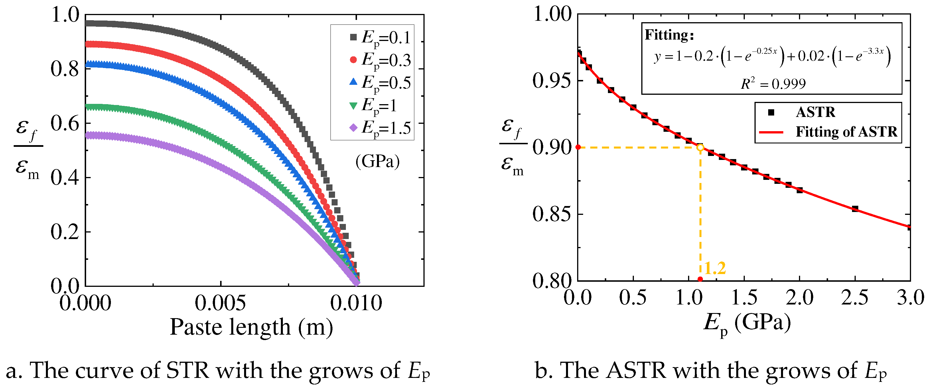
Figure 6. The trend of STR and ASTR with the grows of r_p.

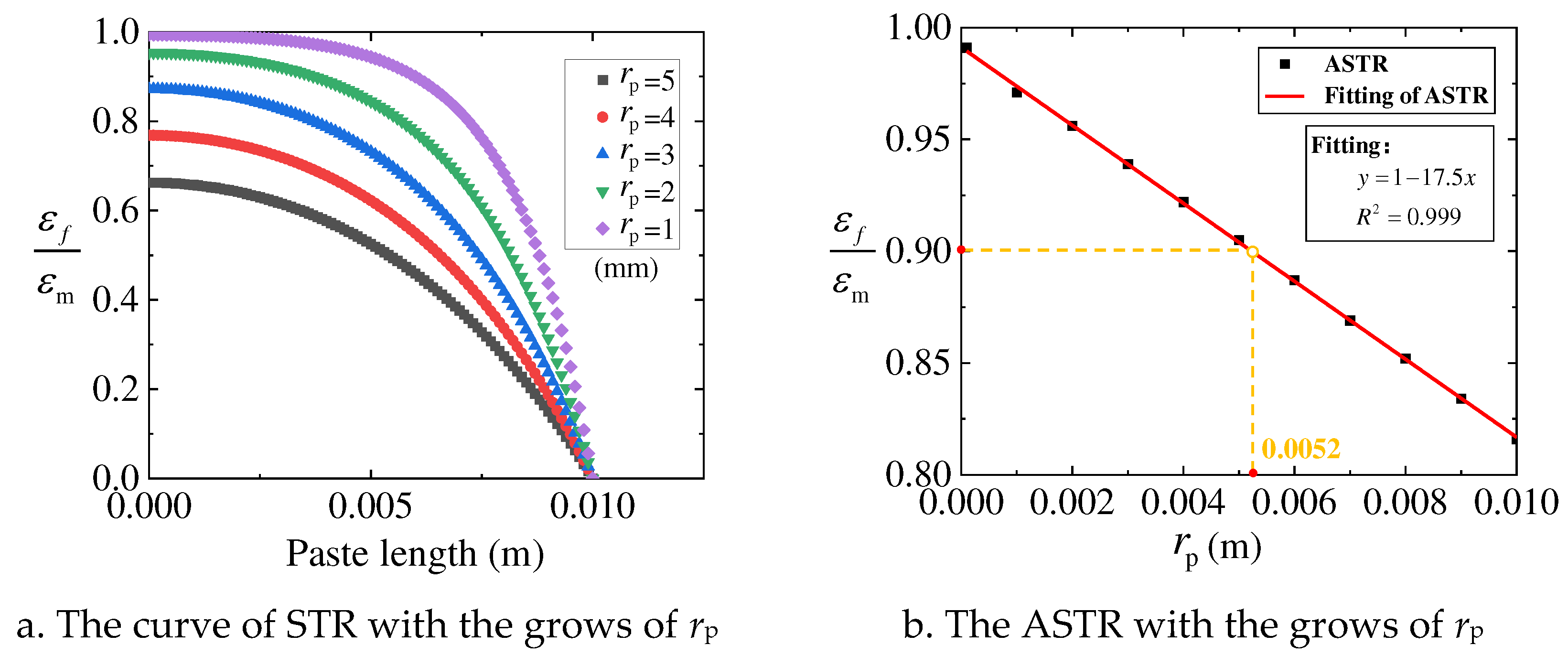
Figure 7. The trend of STR and ASTR with the grows of B.

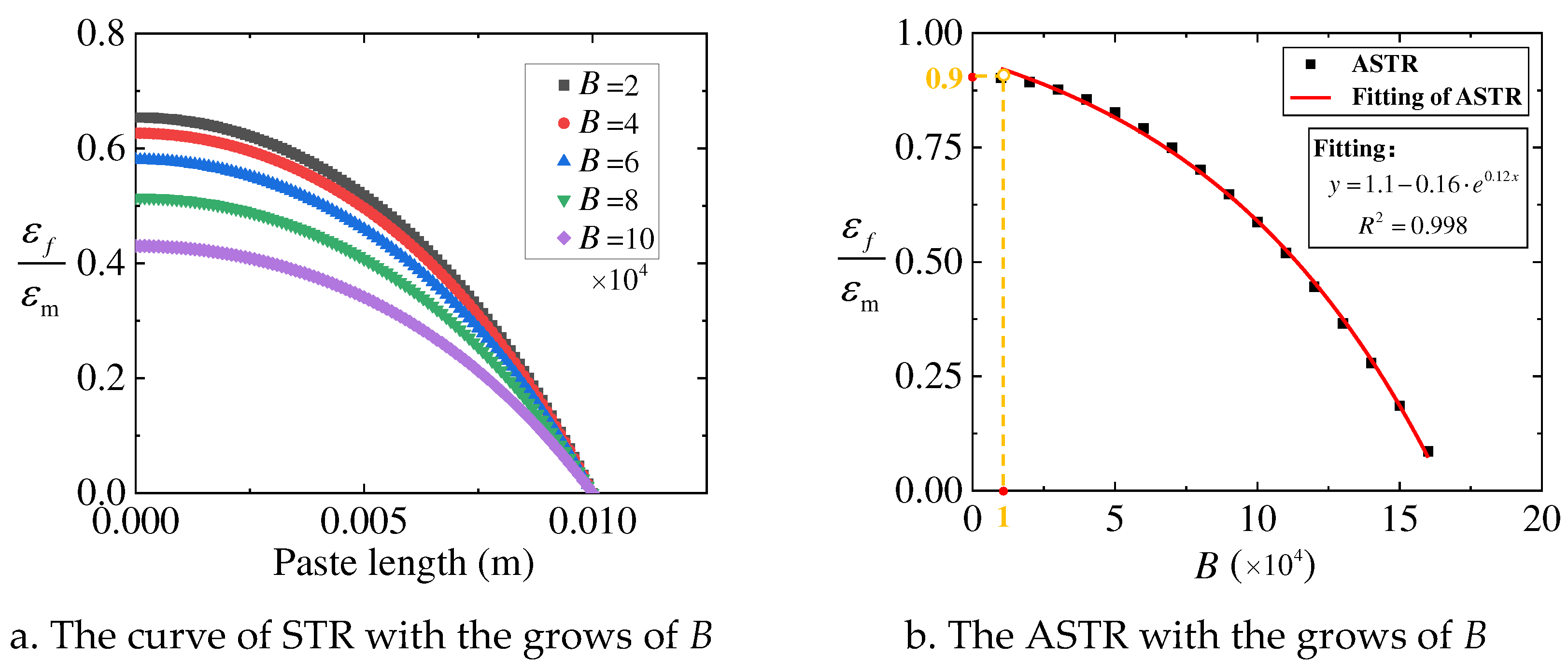
Figure 8. Structure of the calibration device.

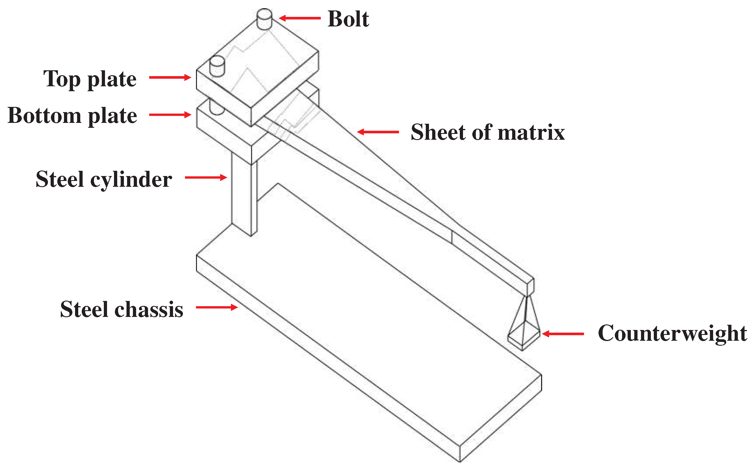
Figure 9. Details of the static calibration test.

Figure 10. Details of the dynamic calibration test.

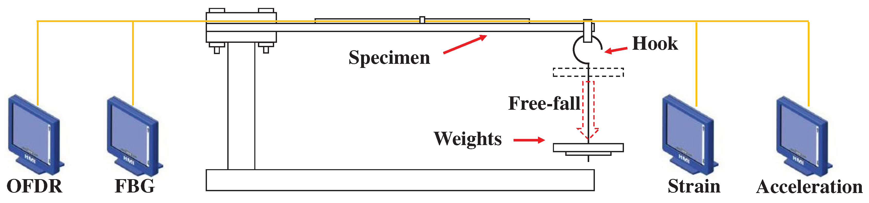
Figure 11. Details of the calibration test.

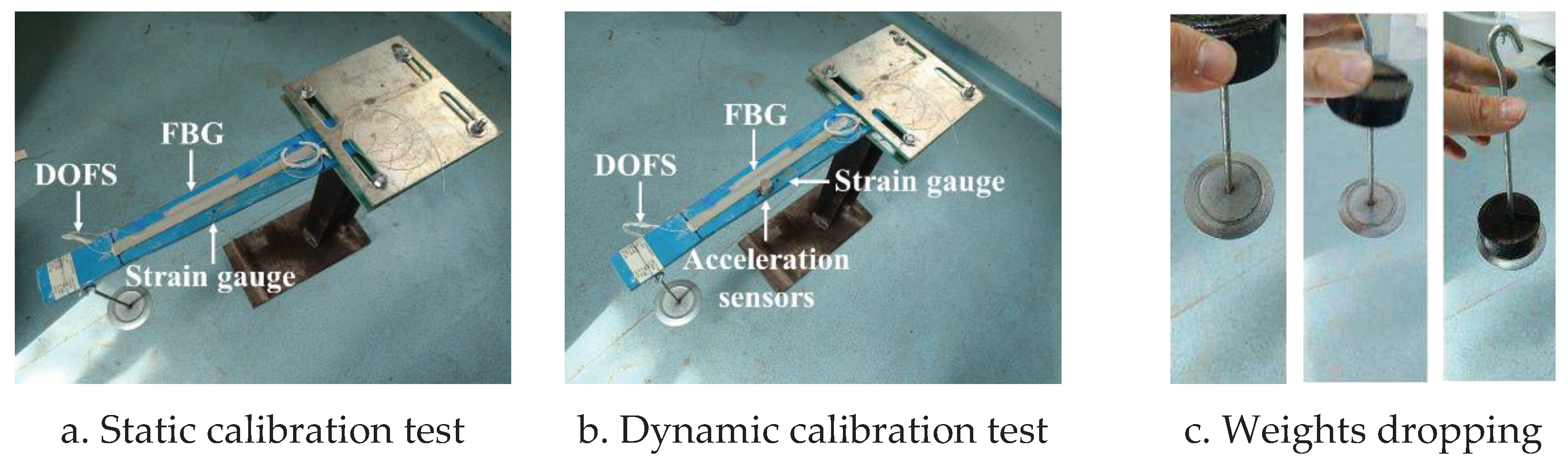
Figure 12. Geometry of the sheet.

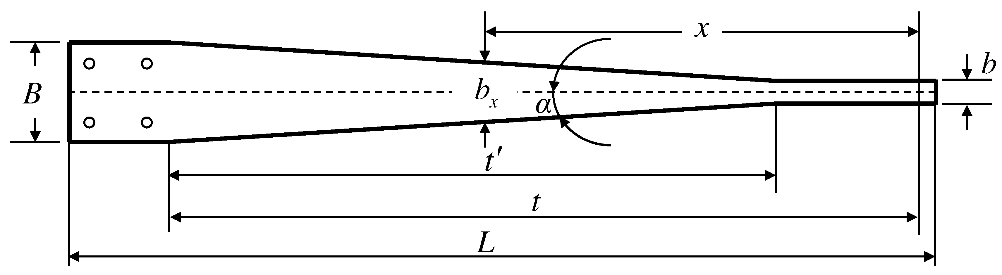
Figure 13. optical fiber sensors in this test.

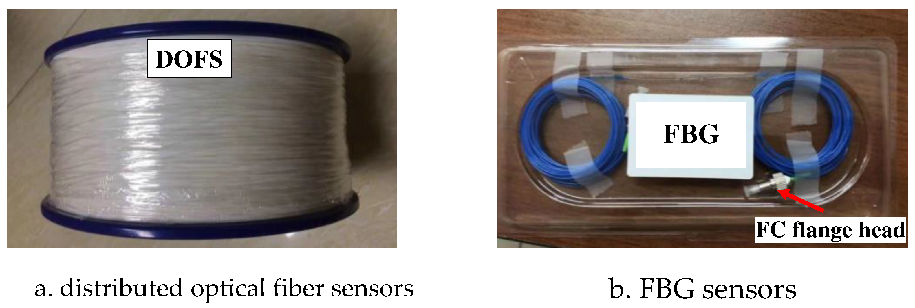
Figure 14. Type of paste method.

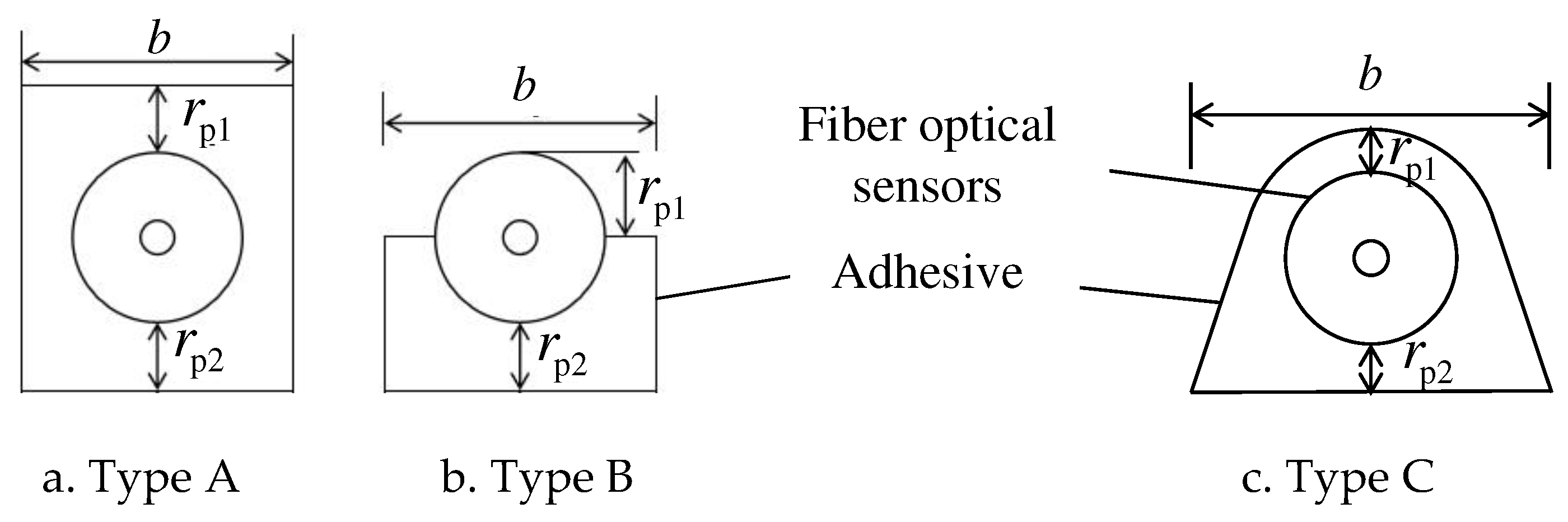
Figure 15. The layout of the optical fiber sensors.

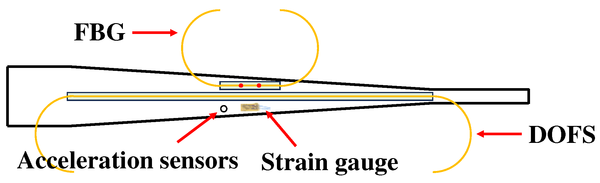
Figure 16. The layout of the optical fiber sensors.

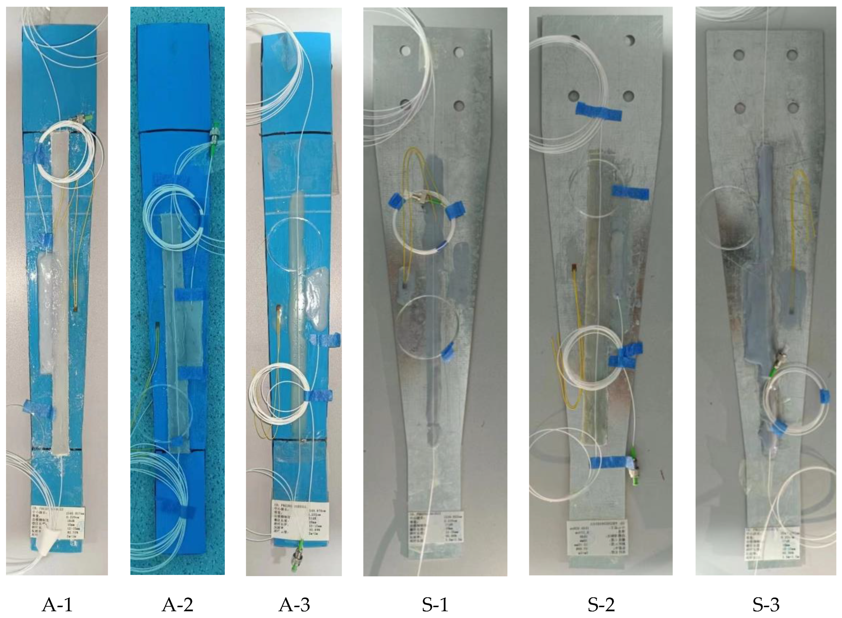
Figure 17. Fiber grating demodulator（Type Zx-fg-c04-1）.

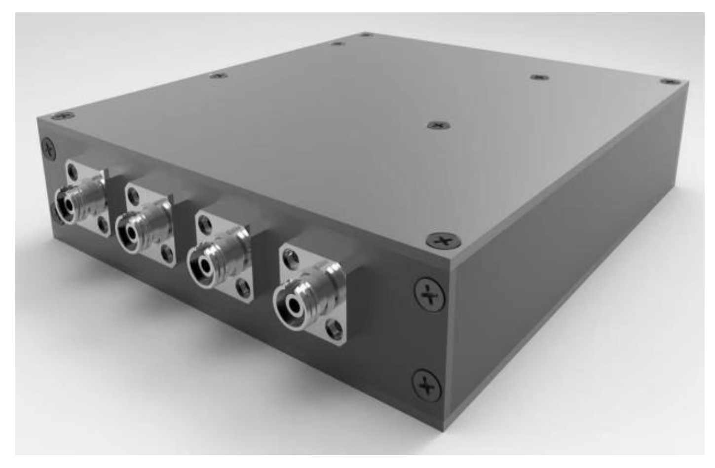
Figure 18. Distributed fiber optic demodulator（Type DITEST STA-R Series）.

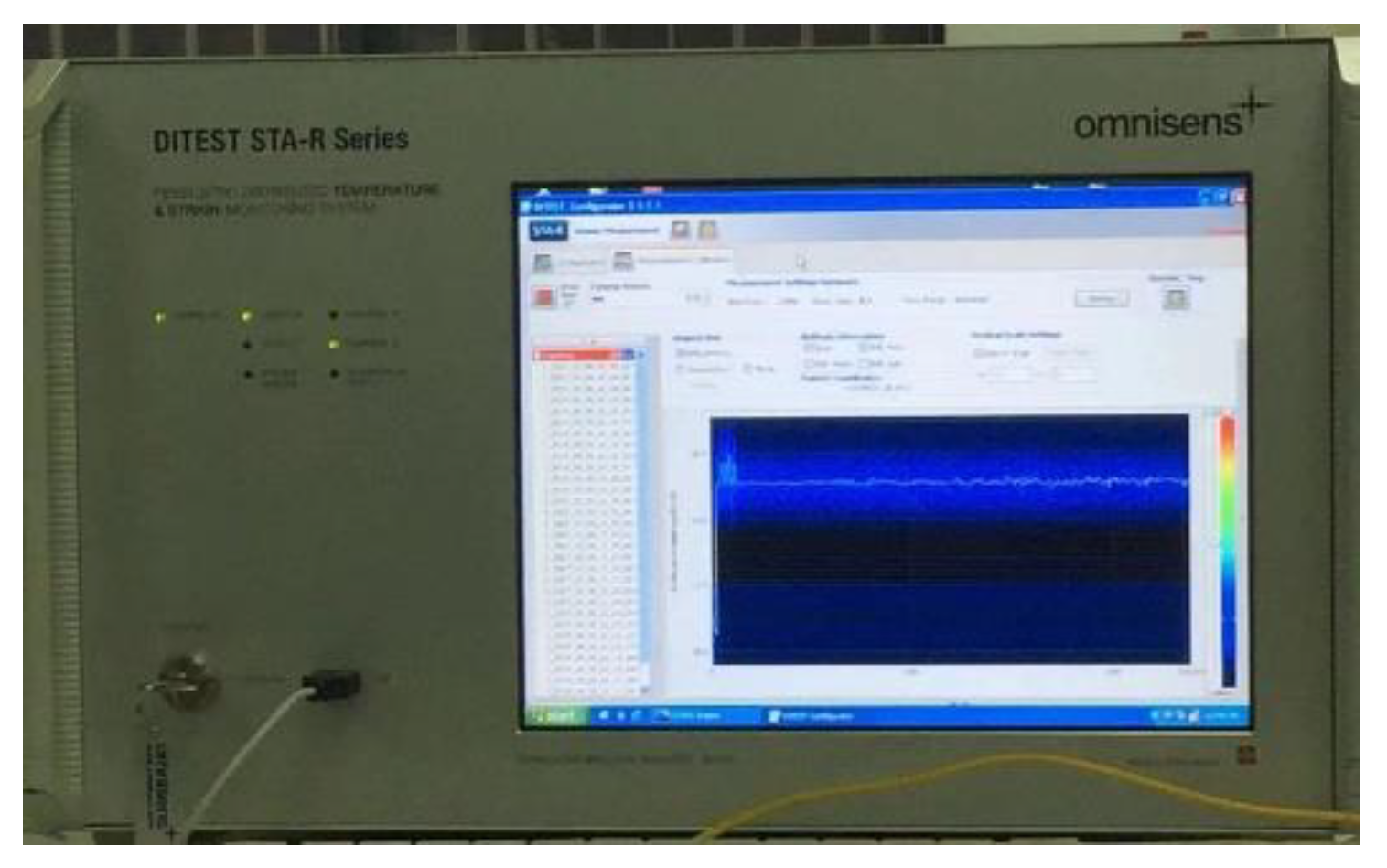
Figure 19. Dynamic distributed fiber optic demodulator（Type OSI-D）.

Figure 20. Dynamic distributed fiber optic demodulator（Type OSI-D）.

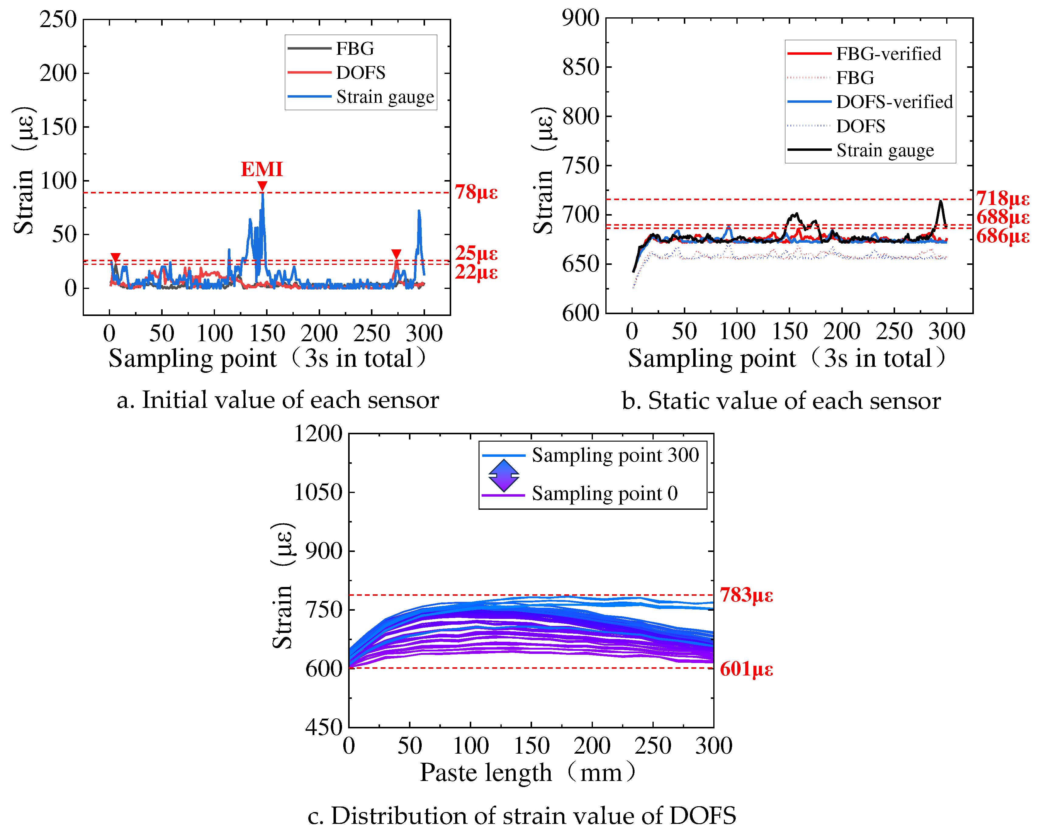
Figure 21. Strain comparison of FBG attached on each sheet.

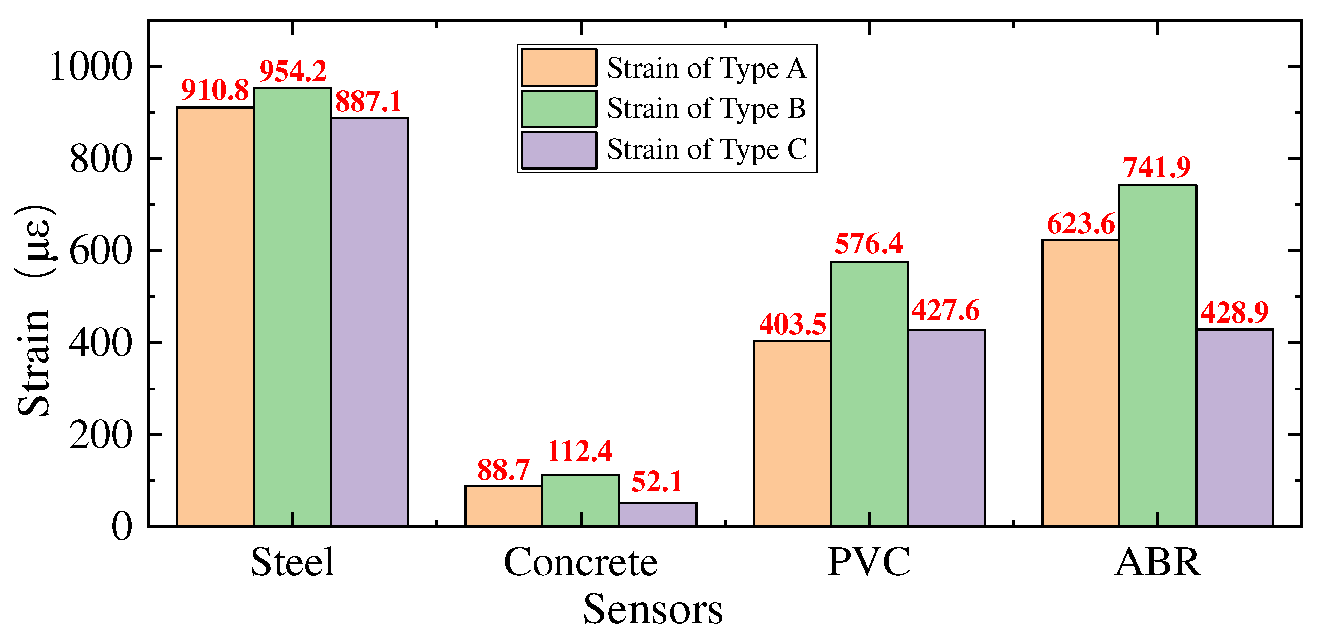
Figure 22. Strain comparison of DOFS attached on each sheet.

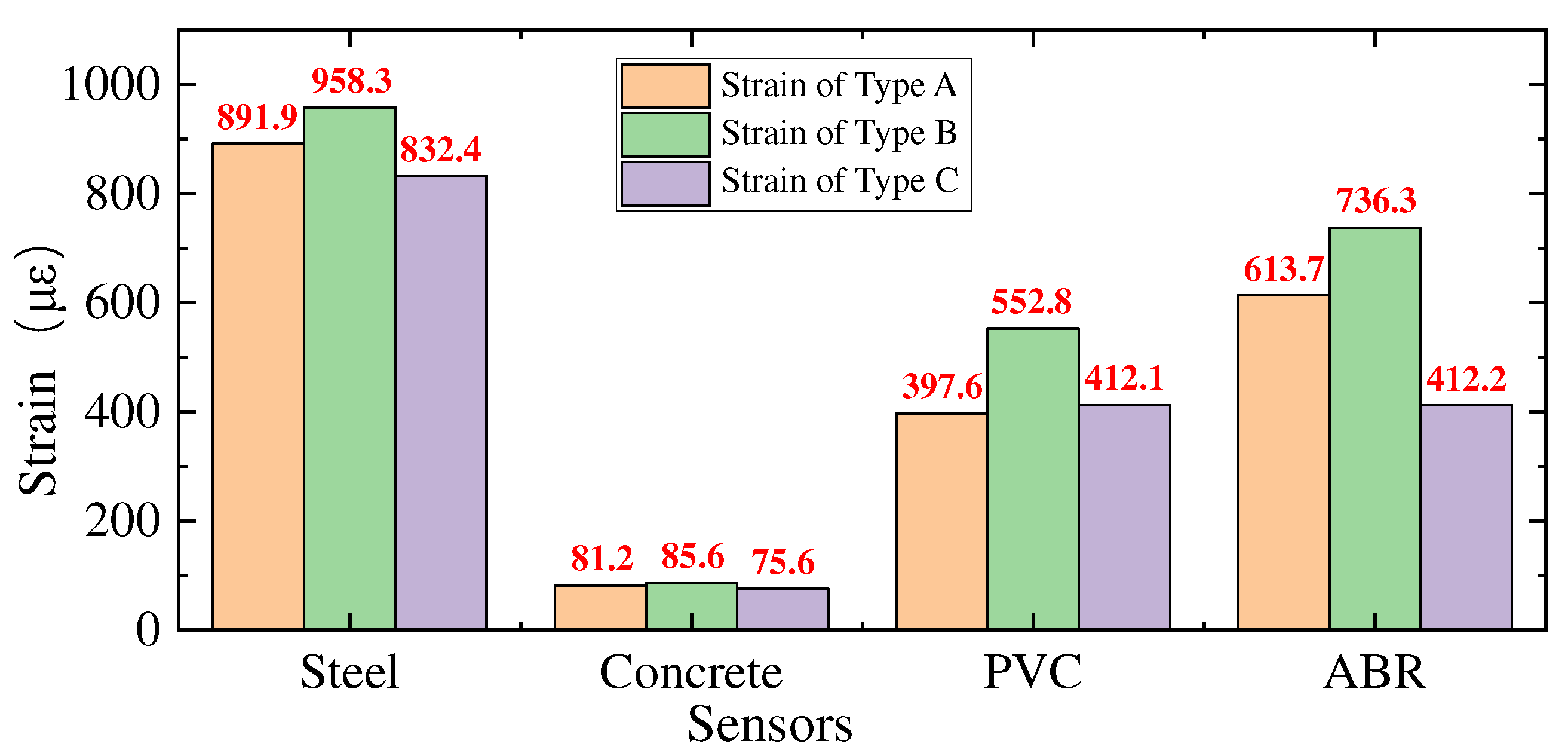
Figure 23. Strain comparison of Strain gauge attached on each sheet.

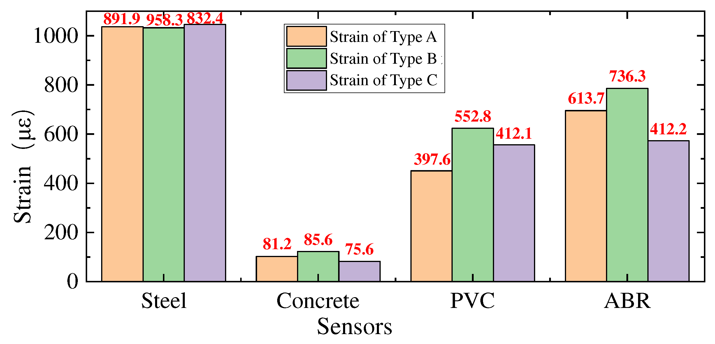
Figure 24. ASTR comparison of sensors attached on each sheet.

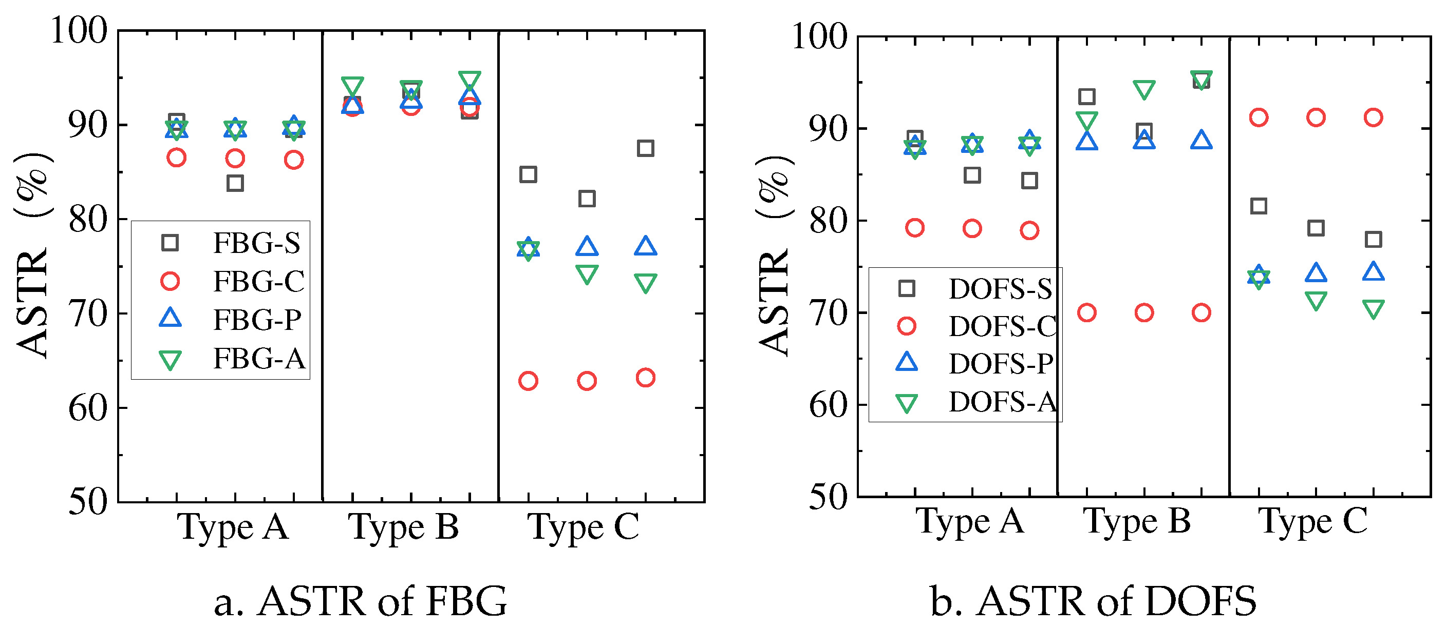
Figure 25. ASTR comparison of sensors attached on the sheet S-1.

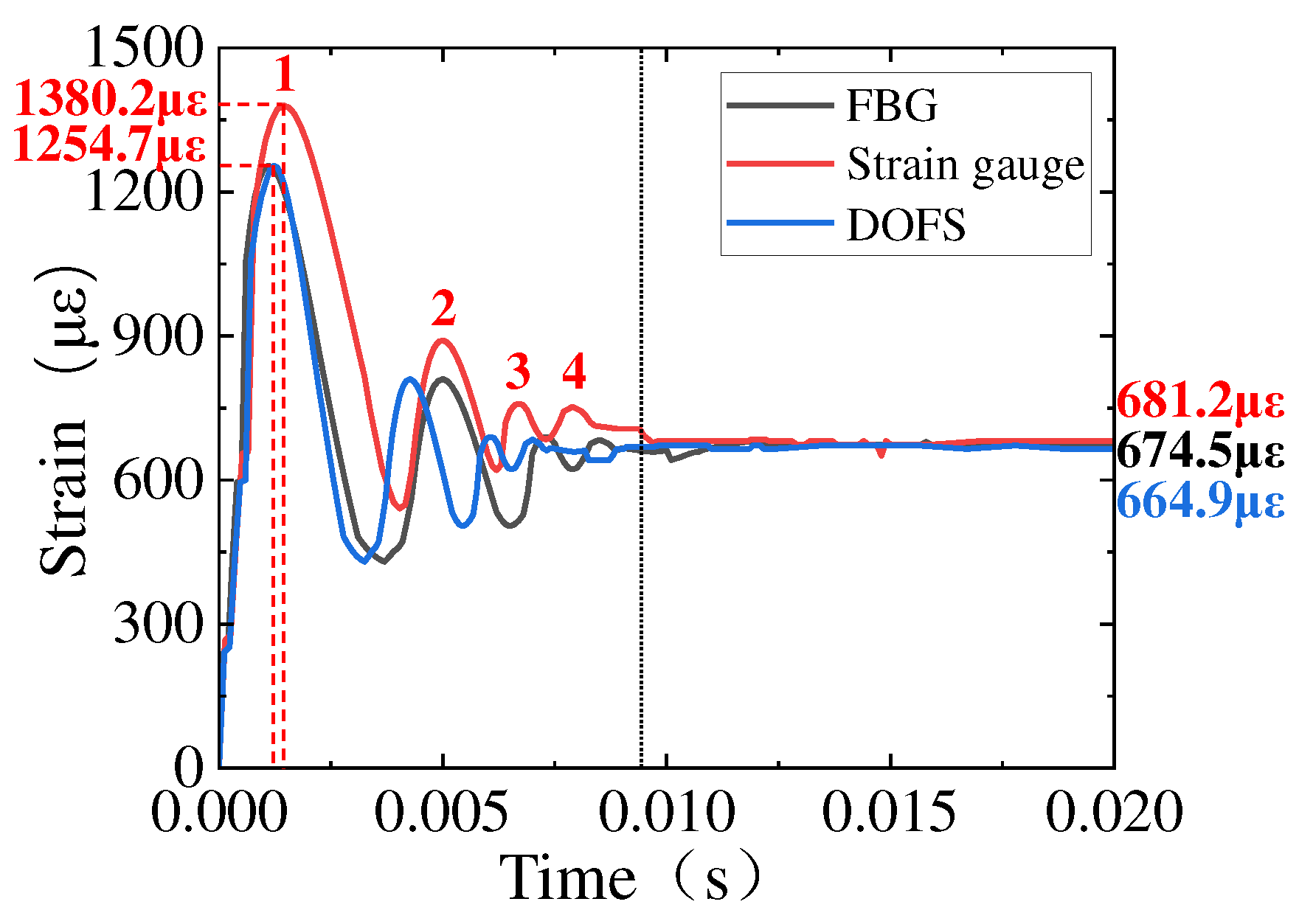
Table 1. Material parameters for theoretical calculation.

Parameters	Fiber core (f)	Protective layer (p)	Adhesive (a)	ABR (m)
E (GPa)	72	0.00255	1	3
r (m)	0.0000625	0.0009	0.005	0.05
v	0.17	0.48	0.38	0.3
ρ (kg/m³)	2200	1200	1200	1200
G (GPa)	30.8	0.00085	0.21	1.154

Table 2. Dynamic parameters for theoretical calculation.

Amplification	Attenuation coefficient	Frequency	Cross-section area
A (kN)	B	f (Hz)	S_m(m²)
100	800	80	0.01

Table 6. Performance of dynamic distributed fiber optic demodulator（Type OSI-D）.

Parameter	Units	Details
Distance	m	20
Spatial resolution	mm	0.64~10.24
Sample rate	Hz	100
Resolution of Temperature	℃	0.4
Resolution of Strain	με	4
Range of Temperature	℃	-200~1200
Temperature of operation	℃	10~40

Tips: Data sourced from Wuhan Megasense Technologies Co.

Table 7. The strain of FBG, DOFS and Strain gauge (Specimen S and C).

Sensors	S-1	S-2	S-3	C-1	C-2	C-3
FBG	903.5	942.5	885.2	88.7	112.4	52.1
	887.5	963.7	863.7	88.7	112.5	52.1
	941.5	956.4	912.4	88.8	112.4	52.4
DOFS	889.2	956.2	852.1	81.2	85.6	75.6
	899.3	923.1	832.4	81.2	85.6	75.6
	887.2	995.6	812.6	81.2	85.6	75.6
Strain gauge	1000.3	1023.2	1044.5	102.5	122.3	82.9
	1058.9	1029.1	1051.2	102.6	122.3	82.9
	1051.8	1045.3	1042.5	102.9	122.3	82.9

Table 8. The strain of FBG, DOFS and Strain gauge (Specimen P and A).

Sensors	P-1	P-2	P-3	A-1	A-2	A-3
FBG	402.9	573.2	427.2	623.5	741.1	427.8
	403.2	576.8	427.7	623.5	741.7	429.5
	404.4	579.3	427.9	623.9	743.1	429.5
DOFS	396.4	551.1	411.1	611.7	715.6	410.8
	397.4	552.1	412.2	614.7	745.6	412.9
	399.1	552.1	412.9	614.7	747.6	412.9
Strain gauge	450.8	623.5	556.2	695.2	785.6	556.4
	450.8	623.6	556.2	695.3	789.4	577.2
	450.8	623.6	556.2	695.9	782.6	584.6

Table 9. The strain of FBG, DOFS and Strain gauge attached on the sheet S-1.

Sensors	1	2	3	4	Average
FBG	1253.2	842.5	702.8	674.5
FBG/ Strain gauge	90.8%	93.5%	93.7%	99.1%	94.3%
DOFS	1254.7	833.6	693.1	664.9
DOFS/ Strain gauge	90.9%	92.6%	92.4%	97.6%	93.4%
Strain gauge	1380.2	900.7	750.4	681.2
FBG/ DOFS	99.9%	101.1%	101.4%	101.4%	101.1%

Table 11. The ASTR of the FBG attached on each sheet.

Specimen	S-1	S-2	S-3	C-1	C-2	C-3
Theoretical results	96.7%	90.8%	87.4%	96.7%	90.8%	60.1%
Test results	88.1%	92.4%	85.2%	87.1%	92.4%	63.1%
Specimen	P-1	P-2	P-3	A-1	A-2	A-3
Theoretical results	96.7%	90.5%	77.8%	96.7%	90.5%	77.8%
Test results	90.5%	92.4%	78.9%	91.1%	93.9%	75.1%

Table 12. The ASTR of the DOFS attached on each sheet.

Specimen	P-1	P-2	P-3	A-1	A-2	A-3
Theoretical results	99.3%	98.2%	97.3%	99.3%	98.1%	90.5%
Test results	86.5%	93.7%	80.1%	79.1%	70.4%	91.4%
Specimen	P-1	P-2	P-3	A-1	A-2	A-3
Theoretical results	99.3%	97.9%	95.8%	99.3%	97.9%	83.3%
Test results	89.8%	88.8%	75.5%	89.2%	95.7%	71.4%

Table 13. The ASTR of the FBG attached on each sheet (Specimen S and C).

Specimen	S-1	S-2	S-3	C-1	C-2	C-3
Theoretical results	90.5%	93.5%	92.1%	90.5%	93.5%	92.1%
Test results	90.1%	92.4%	89.1%	87.8%	96.5%	88.5%
	85.6%	94.2%	88.4%	88.5%	91.2%	89.5%
	88.6%	92.7%	89.6%	93.4%	90.5%	91.5%

Table 14. The ASTR of the FBG attached on each sheet (Specimen P and A).

Specimen	P-1	P-2	P-3	A-1	A-2	A-3
Theoretical results	90.5%	93.5%	92.1%	90.5%	93.5%	92.1%
Test results	91.5%	92.5%	90.5%	93.9%	90.2%	91.6%
	90.1%	92.4%	87.7%	84.1%	90.1%	92.6%
	88.2%	92.1%	94.7%	88.4%	90.1%	91.6%

Table 15. The ASTR of the DOFS attached on each sheet (Specimen S and C).

Specimen	S-1	S-2	S-3	C-1	C-2	C-3
Theoretical results	98.1%	99.5%	99.1%	98.1%	99.5%	99.1%
Test results	91.2%	93.5%	87.5%	77.2%	56.2%	88.1%
	92.4%	94.2%	89.5%	65.2%	92.5%	79.5%
	89.9%	96.5%	74.5%	81.3%	56.9%	85.4%

Table 16. The ASTR of the DOFS attached on each sheet (Specimen P and A).

Specimen	P-1	P-2	P-3	A-1	A-2	A-3
Theoretical results	98.1%	99.5%	99.1%	98.1%	99.5%	99.1%
Test results	77.5%	81.6%	78.4%	65.8%	80.5%	76.8%
	82.9%	96.2%	82.5%	77.5%	92.4%	75.7%
	66.2%	83.3%	87.5%	73.1%	83.7%	88.4%

Disclaimer/Publisher’s Note: The statements, opinions and data contained in all publications are solely those of the individual author(s) and contributor(s) and not of MDPI and/or the editor(s). MDPI and/or the editor(s) disclaim responsibility for any injury to people or property resulting from any ideas, methods, instructions or products referred to in the content.

© 2024 by the authors. Licensee MDPI, Basel, Switzerland. This article is an open access article distributed under the terms and conditions of the Creative Commons Attribution (CC BY) license (http://creativecommons.org/licenses/by/4.0/).

Copyright: This open access article is published under a Creative Commons CC BY 4.0 license, which permit the free download, distribution, and reuse, provided that the author and preprint are cited in any reuse.

Alerts

MDPI Initiatives

Important Links

Choose an area of interest and we will send you notifications of new preprints at your preferred frequency.

Disclaimer