A Systematic Approach to Designing Power Sharing Control of Converter-Based Generators

Mohammad Alomgir Hossain; Md Alamgir Hossain; Hemanshu Roy Pota; Haroldo T. Hattori

doi:10.20944/preprints202401.0923.v1

Preprint

Article

A Systematic Approach to Designing Power Sharing Control of Converter-Based Generators

This version is not peer-reviewed.

Mohammad Alomgir Hossain,

Md Alamgir Hossain^*

Hemanshu Roy Pota

Haroldo T. Hattori

Mohammad Alomgir Hossain,

Md Alamgir Hossain^*

Hemanshu Roy Pota

Haroldo T. Hattori

This version is not peer-reviewed.

Downloads

118

Views

Comments

Submitted:

10 January 2024

Posted:

12 January 2024

You are already at the latest version

A peer-reviewed article of this preprint also exists.

Abstract

This paper introduces a structured design for an effective power-sharing technique among converter-interfaced distributed generation (DG) units within a microgrid that operates without a synchronous generator. The proposed power-sharing technique leverages the battery energy storage system (BESS) to promptly respond to network changes. The real power output of each commercial distributed energy resources (CDER) unit is governed by a frequency-droop characteristic and a complementary frequency restoration strategy. Deloading techniques are employed by solar and wind power generators to enhance response during power supply or demand disturbances. To ensure microgrid stability, small-signal analysis is conducted for controller design, including the determination of stability margins. Initial tuning of the power-sharing technique parameters is achieved using the Ziegler-Nichols Method, followed by further optimization through a meta-heuristical algorithm to enhance the response time of energy sources. The proposed power-sharing technique's performance is evaluated on a benchmark medium voltage network using industry-standard commercial software. The test results demonstrate the precise and rapid power-sharing capabilities among DGs facilitated by the proposed technique, highlighting its effectiveness in dynamic microgrid environments.

Keywords:

distributed generation (DG)

;

battery energy storage system (BESS)

;

doubly-fed induction generator (DFIG)

;

photovoltaic (PV) system

;

DIgSILENT PowerFactory software

;

de-loading technique

Subject:

Engineering - Control and Systems Engineering

Supplementary Material

supplementary.zip (2.04MB )

This preprints belongs to the Topic

Advances in Renewable Energy Technologies and Systems Solutions

1. Introduction

The paradigm of power production in the electrical industry is undergoing a transformative shift from traditional fossil fuel-based sources to renewable energy sources (RES) [1]. Notably, many RES function as distributed generators (DGs) in power networks, interconnected through power electronics converters to enhance network reliability and security [2]. When a low-voltage distribution network operates within a defined area with an amalgamation of DGs, energy storage systems (ESSs), controllers, and loads, it qualifies as a microgrid [3]. The distinctive characteristics of converter-based microgrids set them apart from conventional centralized electrical power generators. Notably, the presence of intermittent energy resources and sources poses a unique challenge, necessitating tailored control strategies. Converter-based DGs inherently exhibit traits such as fast response and reduced inertia, demanding meticulous consideration in the design of controllers aimed at regulating voltage and enhancing power quality for local services [2].

Microgrids operate in two primary modes: (i) grid-connected and (ii) isolated or islanded [4]. In the grid-connected mode, power flow occurs bidirectionally between the microgrid and the main grid to address any disparities between generated power and load demand. Synchronous generators, linked to the primary grid, play a pivotal role in balancing power through the stored energy in rotating inertia, consequently influencing frequency dynamics [5]. In this scenario, Distributed Generators (DGs) within the microgrid function akin to current sources, aligning their voltage frequency with that of the microgrid or grid utility. This synchronization facilitates seamless power exchange between the microgrid and the larger grid utility [6].

Conversely, islanded microgrids operate in isolation from external power grids, rendering power transfer unfeasible during imbalances between supply and demand. In both operational modes, stringent frequency regulation becomes imperative to uphold power balance within the microgrid. This dual-mode operation underscores the versatility and adaptability of microgrids in catering to diverse energy scenarios and requirements.

Household PV systems, when integrated into the microgrid, offer flexibility, allowing installation either with or without battery storage. In certain configurations, these systems can even be leveraged for trading, enabling users to obtain rebates. On the other hand, Commercial DER (CDER) units adhere to established grid codes, emphasizing proper power-sharing mechanisms for ensuring stable operation [7]. Achieving effective power-sharing among CDER units poses challenges, especially in the absence of synchronous generators that traditionally incorporate speed governors to regulate power output in response to demand fluctuations [8]. Given the economic constraints and practical limitations associated with connecting synchronous generators, devising automatic power-sharing strategies becomes imperative for CDER units [9].

Several control approaches have been proposed, with or without the integration of communication lines [10,11,12,13,14], aiming to facilitate proper power-sharing within microgrids [15]. Communication-enabled centralized control has been explored in research such as [16,17], where secondary control sends calculated corrective commands to inverter control units, compensating for frequency deviations. However, studies highlight potential performance degradation in microgrids employing centralized control, attributed to issues like message delays and dropouts [3,18,19,20]. This underscores the significance of robust and distributed control strategies to overcome these challenges and enhance microgrid performance.

In the pursuit of efficient power-sharing within microgrids, various control strategies have been proposed, each offering distinct advantages and addressing specific challenges. However, it’s crucial to critically examine these approaches to ensure their suitability for different operational scenarios. Monshizadeh et al. [6] proposed a communication-free master-slave microgrid, employing a voltage source inverter (VSI) that emulates the behavior of a synchronous generator. Despite its innovative approach, this strategy faces limitations in achieving rapid frequency restoration, potentially jeopardizing network stability. Additionally, the absence of consideration for Phase-Locked Loop (PLL) dynamics in their model poses further challenges. Pota et al. [21] introduced a droop-based controller for power-sharing, assuming an ideal voltage source behind inverters. While this assumption is valid in scenarios involving parallel-connected inverters [22], understanding the true response of renewable energy sources behind ideal voltage sources is essential. Recent literature [23,24] has explored the deloading technique to simulate the inertial response of PV systems for frequency regulation in grid-connected microgrids. Barik et al. [25] proposed a robust controller for a microgrid comprising a PV system, doubly-fed induction generator (DFIG) connected wind generator, and Battery Energy Storage System (BESS) to enhance network stability under islanded operation. However, this approach did not guarantee proper power-sharing among distributed generators. Hossain et al. [10] introduced a novel power control technique employing a voltage band in the DC-link voltage to maintain voltage stability and power quality during temporary disturbances. This approach offers a unique strategy for addressing network challenges. Parvizimosaed et al. [26] presented an intelligent power-sharing (IPS) approach that dispatches active and reactive power among Distributed Generators (DGs) based on droop control gains and operating power capabilities. While promising, this approach relies on communication, adding complexity and cost to the system. In the pursuit of optimal power-sharing, there is a compelling need for an accurate and communication-independent strategy applicable to diverse DG units connected in parallel. This ensures proportional power-sharing, stability, and robust performance in microgrid operations. In [27], a novel grid-forming inverter based on photovoltaic (PV) sources, equipped with modified virtual synchronous machine control, and a battery-supported inverter employing enhanced droop control are introduced. These solutions aim to operate effectively under non-ideal grid voltage conditions and in isolated mode scenarios. However, certain limitations exist, particularly concerning the power-sharing capabilities of the PV inverter during significant demand changes. The assumption of the PV system as an ideal voltage source may hinder its performance in practical implementations. Additionally, both grid-forming and grid-following inverters in [27] contribute to frequency changes during power-sharing, potentially resulting in substantial network frequency variations, especially under dynamic demand conditions.

Despite the contributions of the aforementioned literature, certain drawbacks remain prevalent. These include the assumption of an ideal voltage source for the inverter input, which may not align seamlessly with practical implementations. Moreover, a limited number of papers consider the utilization of the deloading technique to emulate inertial response, and there is a notable absence of model validation using industry-standard software.

To address these gaps, this paper proposes a systematic design of a proportional control strategy for converter-interfaced generators. The developed control algorithm is validated using the PowerFactory-DigSILENT software in a medium-voltage network. The key innovation lies in the application of droop-based control for both grid-forming and grid-following Distributed Energy Resource (DER) units, ensuring proportional power sharing within an islanded microgrid lacking a synchronous generator. Specifically, the Battery Energy Storage System (BESS) with a Pulse Width Modulation (PWM) inverter is designated as grid-forming, while PV systems and Doubly Fed Induction Generators (DFIG) serve as grid-following components.

In order to assess the stability of the proposed controller, a dynamic model is developed for a multiple-Distributed Generation (DG) microgrid, focusing on small-signal dynamics. Sensitivity analysis is conducted after linearizing the model and selecting operating point parameters. Given the potential challenges in large inverter-based microgrids, the Ziegler-Nichols (ZN) and particle swarm optimization (PSO) methods are employed. These methods aid in accurately determining the suitable range for the designed droop parameters. Through the analysis, it is evident that the proposed technique adeptly achieves precise and swift power sharing among Energy Internet-Connected DG (EI-DG) units. This approach facilitates optimal power allocation in accordance with the units’ power ratings and eliminates the need for individual Battery Energy Storage Systems (BESS) for each DER unit.

The main contributions of this study are shown as follows.

Equitable Load Distribution Controllers: Development of specialized controllers designed to facilitate fair distribution of load changes among Distributed Generation (DG) units, taking into account the ratings of Distributed Energy Resources (DER) units within the microgrid. Two distinct controller types are formulated for this purpose: (1) a grid-forming controller, intricately connected to the Battery Energy Storage System (BESS); (2) a grid-following controller, specifically designed for DER units.
Optimal Coefficient Determination for Droop Controllers: Identification and optimization of the key coefficients for droop controllers, a critical aspect ensuring the stability of the system. The aim is to achieve: (1) system stability under varying conditions; (2) swift restoration of the frequency to its nominal value following disturbances; and (3) proportional power sharing among DER units, aligning with their individual power ratings.
Small-Signal Analysis for Stability: Implementation of small-signal analysis to finely tune the control parameters, offering a deeper understanding of the system’s stability margin. This analysis contributes to the robust design of controllers, improving the microgrid’s responsiveness.
Thorough Performance Validation: Rigorous testing and validation of the proposed power-sharing technique on a benchmark medium voltage network using industry-standard commercial software. The results demonstrate the accuracy, speed, and effectiveness of the proposed technique in sharing power among DGs.

This novel approach seeks to overcome the limitations observed in previous literature, offering a more practical and validated solution for microgrid control in real-world applications.

The rest of this paper is arranged as follows. Section II briefly describes the generic system model where the cases are studied. The proposed control for power-sharing has been described in section III. Sections IV deals with general small-signal analysis after linearization of the model and a method to determine the co-efficient of the proposed controllers. Section V shows the simulation results after implementing the proposed algorithm for 4 and 9 bus systems. Moreover, Section VI concludes the results obtained from the analysis of the study system.

2. System overview

A microgrid consisting of several Power-electronics elements can operate in parallel, grid-connected, or islanded mode. Figure 1 shows a general structure of the microgrid, which consists of one-off BESS and n DER units. The microgrid is connected to the utility system through a static transfer switch (STS) at the point of common coupling (PCC). As depicted in Figure 1, each DER unit comprises a renewable energy source (RES).

Moreover, a power electronic interface is comprised of a dc-ac inverter. Each DER can be directly connected to a predefined load or to the ac common bus to supply power. Now, for the network shown in Figure 1, the complex power can be written as:

S_{i} = P_{i} + j Q_{i} = V_{i} ∠ δ_{i} \times I_{i} ∠ - φ_{i}, i = 1, 2, 3, 4 . . n

(1)

Also,

I_{i} ∠ φ_{i} = \sum_{j = 1}^{n} Y_{i j} V_{j} ∠ δ_{j}

(2)

Where,

$S_{i}$ is the complex power at i-th bus
$P_{i}$ is the active power at i-th bus
$Q_{i}$ is the reactive power at i-th bus
$V_{i}$ is the voltage at i-th bus
$I_{i}$ is the current at i-th bus
$δ_{i}$ is the current angle at i-th bus
$φ_{i}$ is the current angle at i-th bus

The currents and voltages of the micro-grid buses shown in Figure 1 are related to:

Y_{b u s} V_{b u s} = I_{b u s}

(3)

where,

Y_{b u s} = [\begin{matrix} Y_{11} & \cdot & \cdot & Y_{n n} \\ \cdot & \cdot & \cdot & \cdot \\ \cdot & \cdot & \cdot & \cdot \\ Y_{1 n} & \cdot & \cdot & Y_{n n} \end{matrix}]

(4)

V_{b u s} = [\begin{matrix} V_{1} ∠ δ_{1} \\ ⋮ \\ V_{n} ∠ δ_{n} \end{matrix}], I_{b u s} = [\begin{matrix} I_{1} ∠ Φ_{1} \\ ⋮ \\ I_{n} ∠ Φ_{n} \end{matrix}]

(5)

The equation for the active power at i-th bus can be written as follows:

P_{i} = \sum_{k = 1}^{n} Y_{i k} V_{i} V_{k} cos (θ_{i k} + δ_{k} - δ_{i})

(6)

where

θ_{i k}

is the angle of the impedance

Y_{i k}

2.1. BESS Model

The dc/ac inverter connected to the BESS is classified as grid forming voltage source inverters (VSIs). The control mode of the PWM converter connected to the BESS is Vac-phi where the terminal voltage magnitude and phase are specified. The main purpose of BESS is to provide a fast frequency regulation response and share the load burden of conventional power generation units.

With Vac-phi control mode, the existing BESS does not have the specified active power set point. The BESS is connected to the slack bus (bus no. 1), and if there is any load change event that happens, the active power changes as per the load flow Eq. (1)-(6).

The selection of BESS over other energy storage devices is based on several factors that make BESS well-suited for the proposed research. BESS offers advantages such as fast response times, high efficiency, and the ability to provide both active power support and energy storage. Additionally, BESS technology has been widely adopted in various power systems and microgrid applications, making it a practical and established choice for addressing power-sharing, stability, and frequency control challenges in the context of this research. The decision to focus on BESS is rooted in its proven performance, versatility, and relevance to contemporary power system applications.

2.2. DER Model

Due to the high prevalence of RESs, frequency stability challenges are significant [28], as RESs tend to have low or no inertial responses [29]. For example, solar photovoltaic plants do not provide an inertia response to the power grid. On the other hand, variable-speed wind turbines are usually connected to the grid via power electronic converters, freeing them from power system transients. As a result, replacing traditional sources with renewable energy sources will reduce the inertia of the entire power system. For this reason, the frequency deviation will increase, as reported in [30]. This section describes the use of deloading technique for solar PV and wind turbines from literature to overcome the frequency stability challenges. In this paper, deloading technique has been used for proportional power-sharing.

2.2.1. PV System

In PV systems, there are two parts[31]: solar conversion and electronic conversion. Figure 2 shows the inverter (dc-ac converter) connects PV arrays to loads via a dc-dc converter (boost converter). A dc-dc boost converter achieves the maximum output power conversion from the PV array to the inverter, and an inverter converts that power into ac to supply the ac load.

Most of the PV systems operate in the maximum power operation region to obtain an energy benefit. The system proposed in [23,32] is one in which a few systems work away from the MPPT point to provide for a margin of available reserve power. In Figure 4, how de-loading provides a cushion for active power-sharing is represented. PV arrays can maintain some reserve power by increasing

V_{M P P}

by voltage

V_{d e l}

Until the system’s frequency deviates from its nominal value, this reserve power will not be released. A control signal proportional to the frequency deviation

V_{d c Δ f}

is added to the DC reference voltage under these conditions. In Figure 5, it is clear that the change in the direct current

i_{d r e f}

, i.e., output power of a PV depends on the

V_{M P P}

value and the frequency deviation, as demonstrated by Eq. (7).

V_{d c r e f} = V_{M P P} + V_{d e l} - V_{d c Δ f}

(7)

Figure 4 also shows how the PV voltage is maintained at point 3 to keep some reserve power. When the system frequency decreases, a control signal related to the frequency deviation reduces the PV voltage and makes it operate at point 2. The PV voltage is then forced to operate at a point away from the MPPT one by using the deloading technique so that a

P_{r e s}

is available in the system. This reserve is used to attribute the inertial response to the PV generator to share the active power when an active power change occurs in the network. How much active power can be shared depends on the reserve available in the system. In de-loaded condition, if

P_{r e s}

is the available reserve:

P_{r e s} = P_{M P P} - P_{g r i d}

(8)

where

P_{M P P}

is the power output at the MPPT point and

P_{g r i d}

the power injected into the grid. The change in the active power load triggers the BESS controller to change the frequency of the network. This can be compensated by making use of the reserve as:

P_{r e s} = Δ f . G a i n

(9)

2.2.2. DFIG-connected Wind Power Generator

Figure 6 shows how wind turbines are typically coupled with a DFIG to transform wind energy into electrical power. Firstly, its wind blades create a mechanical torque in the rotor shaft of the induction generator. Then, a set of Back to Back converters is fed from the grid to the induction generator to, control the generator’s real and reactive power outputs. [25].

Optimal power extraction curves are used to design wind turbines from an economic standpoint. As a result, it does not participate in power-sharing or frequency regulation. Therefore, the system must have adequate reserve capacity to handle any frequency variations. De-loading is a new technique for ensuring a reserve margin by altering the wind turbine’s operating point from its optimal power extraction curve to a lower power level. De-loading can be achieved by increasing the blade’s angle. In Figure 7, the power-rotor speed curves of a DFIG wind turbine running at point A under different pitch angles are shown. The pitch angle controller increases the angle of the wind turbine’s blades and moves the operating point from A to B despite any variation in the rotor’s speed.

2.3. PLL

PLLs are frequently used for synchronization and controller functions. They can also be used for frequency-modulated signals[34]. The phase-locked loop element measures the frequency and phase of a voltage in the system. Figure 8 shows the PLL block diagram used in the DigSILENT Power Factory software[35].

DIgSILENT PowerFactory is a program designed to analyze transmission, distribution, and industrial electrical power systems. The main objective of the software is to plan and optimize operations. It is designed as an advanced integrated and interactive software package for the electrical power system and control analysis. The accuracy and validity of Power Factory’s results have been confirmed by many organizations involved in the planning and operation of power systems worldwide[35].

From Figure 8 we can see the block diagram of the PLL to measure the frequency of the network.

It can be seen that the dynamics of the PLL for measuring the frequency of the network is:

Δ f_{i} = k_{p}^{P L L} Δ δ_{i} + k_{i}^{P L L} \int Δ δ_{i}

(10)

where

k_{p}^{P L L}

and

k_{i}^{P L L}

are the proportional and integral coefficients of the PLL, respectively,

Δ f_{i}

denotes frequency change while

Δ δ_{i}

changes the angle at the i-th bus. In this paper. as the value of

k_{i}^{P L L}

is chosen as almost zero, Eq. (10) can be written as:

Δ f_{i} = k_{p}^{P L L} Δ δ_{i}

(11)

2.4. Observations

All the DER units are connected to the PV bus. So, there is an initial active power set-point for all DER units. However, all the DER units are capable of changing the active power set-point if there is any frequency deviation in the network to restore the system frequency to nominal value.

The synchronous generator connected to the main grid balances the power from the power stored in the rotating inertia, resulting in a change in frequency in the network. As there are no synchronous generators connected to the network as per Figure 1, so there is no change in frequency in the network. The BESS is connected at slack bus no 1 through a grid-forming inverter. So, any active power demand change in the network will be balanced by BESS. All other connected DER units will not participate in the power sharing and there is a necessity to implement a new controller to make sure all other DER units are participating proportionally.

3. Proposed power sharing

The load-sharing method proposed in this paper is designed to operate in the absence of a synchronous generator, where changes in inertia directly impact frequency. In such a scenario, the absence of a synchronous generator means that changes in load demand won’t lead to frequency variations in the network. To address this, the grid-forming DER unit is assigned the responsibility of inducing frequency changes in response to variations in power demand. All other grid-following inverters then utilize the frequency changes initiated by the grid-forming DER unit as feedback to ensure proportional power sharing.

There is no frequency change in the network as there is no synchronous generator connected to it. In this proposed controller, the system utilizes the deviation of the frequency as a control variable. This essentially conveys information to the local controller regarding the consumption/generation balance of the grid. However, the frequency change in the network is facilitated by the grid-forming inverter connected to the BESS, depending on the demand load changes in the network. The alteration in active power demand is measured by the active power measurement device connected to the slack bus (bus-1). The new frequency is then set by the converter connected to the BESS, following the equations (12) and (13) presented in sub-section 3.1. The connected DER units function as grid followers, responding to frequency changes in the network to ensure power sharing among the DER units. Phase-Locked Loops are connected to all DER units to measure the new frequency and frequency deviation, serving as control variables for the new active power set point of the DER units. The subsequent sections provide detailed information on the proposed controllers.

3.1. BESS

The main purpose of a BESS is to provide a fast frequency regulation response and share the load burden of conventional power generation units. Figure 9 shows the proposed control structure of the grid-forming inverter connected to the BESS.

As per this figure, the new frequency is defined by:

f_{1, n e w} = f_{1} + k_{p r, 1} (P_{1} - P_{m 1}) + k_{q r, 1} (f_{m 1} - f_{1})

(12)

where

f_{1, n e w}

is the new reference frequency of the BESS,

f_{1}

reference frequency,

f_{m 1}

the measured frequency,

k_{p r, 1}

proportional droop co-efficient of BESS for a frequency change,

k_{q r, 1}

proportional droop co-efficient for its power sharing,

P_{m 1}

measured output power and

P_{1}

reference output

As, in Eq. (12) there are two droop co-efficient

k_{p r, 1}

and

k_{q r, 1}

, with a change in load the frequency can be changed and, at the same time, power can be shared. In a normal mode of operation, when all the connected DER units are capable of sharing the active power, the BESS doesn’t share and

k_{q r, 1} = 0

. Nevertheless, when the DER units are capable of sharing the power with a change in load, the BESS changes the value of

k_{q r, 1}

. In this paper, the non-active power-sharing mode of a BESS is emphasized and a small-signal analysis is performed based on it. Therefore, Eq. (12) can be simplified to:

f_{1, n e w} = f_{1} - k_{p r, 1} (P_{1} - P_{m 1})

(13)

Furthermore, the VSI connected to the slack bus acts as a synchronous generator and changes its voltage frequency according to changes in loads. This is almost the same as the inertial response of the synchronous generator which can ensure proper sharing of the active power among the DER units. All the connected DER units respond to frequency changes in the network; for example, the frequency will decrease if the DGs supply more than the load demand of the network and vice-versa. Later, the grid-following inverters respond to frequency deviations and ensure power-sharing at the same time. The new frequency generated by the VSI of the BESS is measured by the PLLs of all the grid-following DER units connected to the network. As the frequency changed by the BESS will be the same in all the buses and no other DER units change the frequency of the network,

Δ δ_{i} = Δ δ_{1}

Please note that we assume that the BESS has the capability to adjust its State of Charge (SOC) based on changes in power demand. We acknowledge the importance of considering the dynamic behavior of SOC in the power management strategy, especially when reaching lower or upper limits, which will be explored in future work.

3.2. DER units

All the connected DER units are considered dispatchable and grid following. Therefore, they have their own local controllers to share the active and reactive powers. The control structure of all these units is shown in Figure 10.

Then, the equation for active power sharing is:

\begin{matrix} Δ P_{i} (s) = Δ f_{i} (s) (\frac{1}{1 + s T}) (k_{p r . i} + \frac{k_{i n . i}}{s}) [i \neq 1] \end{matrix}

(14)

where,

Δ P_{i} = P_{r, i} - P_{r, n e w}

is a change in the active power set-point,

Δ f_{i} = (f_{m, i} - f_{r, i})

represents the measured change of frequency at the i-th bus,

k_{p r, i}

is the proportional droop coefficient of the DER unit at the i-th bus,

k_{i n, i}

is a different coefficient related to the DER unit at the i-th bus, and T is the time coefficient.

Therefore, the active power set points of the DER units change as per Eq. (14). To ensure proper power sharing according to the power ratings of DER units, the droop coefficients can be selected as [7]:

P_{n}^{r} k_{p r, m} = P_{m}^{r} k_{p r, n}

(15)

P_{n}^{r} k_{i n, m} = P_{m}^{r} k_{i n, n}

(16)

where

P_{m}^{r}

and

P_{n}^{r}

are the rated power of the DER units connected to m-th and n-th buses, respectively.

In this paper, the proposed algorithms are implemented in a 9-bus network in which there are a BESS and 2 off DER units (DFIG -connected wind power generator and PV system). Their inverters connected to the BESS are grid -forming whereas the inverters connected to DER units are grid-following. All the controller’s coefficients are evaluated in section 3.

4. Linearised model and gain selection

To study the electro-mechanical oscillations and understand the dynamic characteristics of a system, a small-signal analysis is widely used [36]. The main goal of this method is to linearize a system model’s equations to stable or unstable equilibrium points [37] and later eigenvalues are evaluated to check the stability [38]. In this section, an L-type micro-grid is linearized to real power versus frequency and its eigenvalues also determined. This linearized model is developed considering only one grid-forming inverter connected to a BESS and an indefinite number of grid-following ones connected to DER units. This model is then used for 4 and 9 bus systems to tune the control parameters and gain a better understanding of the dynamics of a micro-grid with the proposed control.

4.1. Linearised model

δ_{i} - δ_{i}^{0} = Δ δ_{i}

δ_{i k} = δ_{i} - δ_{k}

, and

Δ P_{i} = P_{i} - P_{i}^{0}

are considered and a Taylor series is used to expand Eq. (6) up to 1^st order[39], then it can be written as follows:

[\begin{matrix} Δ P_{1} \\ Δ P_{2} \\ . \\ . \\ . \\ Δ P_{n} \end{matrix}] = [\begin{matrix} a_{11} & a_{12} & . & . & . & a_{1 n} \\ a_{21} & a_{22} & . & . & . & a_{2 n} \\ . & . & . & . & . & . \\ . & . & . & . & . & . \\ . & . & . & . & . & . \\ a_{n 1} & a_{n 2} & . & . & . & a_{n n} \end{matrix}] [\begin{matrix} Δ δ_{1} \\ Δ δ_{2} \\ . \\ . \\ . \\ Δ δ_{n} \end{matrix}]

(17)

where,

a_{i j} = {\frac{\partial P_{i}}{\partial δ_{j}}|}_{(.) = {(.)}^{0}}

and

i = 1, 2, 3 . . . . n

where

(.) = {(.)}^{0}

means that a function is evaluated at the equilibrium value of all the variables.

Defining,

Δ P_{m i} = P_{m i} - P_{i}^{0}

as a linear representation of the system described by Eq. (13):

Δ f_{1} = k_{p r, 1} Δ P_{m 1}

(18)

The relationship between the voltage’s frequency and angle can be written as[21]:

Δ f_{1} = Δ \dot{δ_{1}}

(19)

from Eqs. (18) and (19):

Δ \dot{δ_{1}} = k_{p r, 1} Δ P_{m 1}

(20)

After a Laplace transform, Eq. (20) can be written as:

s Δ δ_{1} (s) = k_{p r, 1} Δ P_{1} (s)

(21)

The DER units connected to the network deviate from their active power set-points as per Eq. (14) that is,

Δ P_{i} (s) = k_{p r, 1} Δ f_{1} (s) (\frac{1}{1 + s T}) (k_{p r, i} + \frac{k_{i n, i}}{s}) [i \neq 1]

(22)

The amount of power to be shared

Δ P_{i}

is calculated by Eq. (22). Replacing

Δ f_{i} (s)

using Eq. (11), this Eq. (22) is re-written as:

Δ P_{i} (s) = k_{p 1} Δ δ_{i} (s) (\frac{1}{1 + s T}) (k_{p r . i} + \frac{k_{i n . i}}{s}) [i \neq 1]

(23)

Now, Eq. (30) can be written as:

[\begin{matrix} Δ δ_{1} \\ Δ δ_{2} \\ . \\ . \\ . \\ Δ δ_{n} \end{matrix}] = {[\begin{matrix} a_{11} & a_{12} & . & . & . & a_{1 n} \\ a_{21} & a_{22} & . & . & . & a_{2 n} \\ . & . & . & . & . & . \\ . & . & . & . & . & . \\ . & . & . & . & . & . \\ a_{n 1} & a_{n 2} & . & . & . & a_{n n} \end{matrix}]}^{- 1} [\begin{matrix} Δ P_{1} \\ Δ P_{2} \\ . \\ . \\ . \\ Δ P_{n} \end{matrix}]

(24)

Let,

{[\begin{matrix} a_{11} & a_{12} & . & . & a_{1 n} \\ a_{21} & a_{22} & . & . & a_{2 n} \\ . & . & . & . & . \\ . & . & . & . & . \\ a_{n 1} & a_{n 2} & . & . & a_{n n} \end{matrix}]}^{- 1} = [\begin{matrix} b_{11} & b_{12} & . & . & b_{1 n} \\ b_{21} & a_{22} & . & . & b_{2 n} \\ . & . & . & . & . \\ . & . & . & . & . \\ b_{n 1} & b_{n 2} & . & . & b_{n n} \end{matrix}]

(25)

From Eqs. (24) and (25):

\begin{matrix} Δ δ_{1} = b_{11} Δ P_{1} + b_{12} Δ P_{2} + . . . . . + b_{1 n} Δ P_{n} \end{matrix}

(26)

The Laplace transform of Eq. (26) is:

\begin{matrix} Δ δ_{1} (s) = b_{11} Δ P_{1} (s) + b_{12} Δ P_{2} (s) + . . . . . + b_{1 n} Δ P_{n} (s) \end{matrix}

(27)

Considering the variable load connected to the n-th bus and the grid following DER units connected to all other buses except 1:

\begin{matrix} Δ δ_{1} (s) - [b_{11} Δ P_{1} (s) + b_{12} Δ P_{2} (s) + . . . . . + b_{1 (n - 1)} Δ P_{n - 1} (s)] \\ = b_{1 n} P_{L} (s) \end{matrix}

(28)

Solving Eqs. (21), (22) and (27), it can be found:

\frac{Δ δ_{1} (s)}{Δ P_{L} (s)} = \frac{E s^{2} + F s}{L s^{3} + M s^{2} + N s + O}

(29)

where,

E = b_{1 n} k_{p r, 1} T

F = b_{1 n} k_{p r, 1}

L = - T b_{11}

M = - (b_{11} + T k_{p r, 1})

N = k_{p r, 1} [1 + k_{p}^{P L L} (b_{12} k_{p r, 2} + . . . + b_{1 (n - 1)} k_{p r, (n - 1)})]

and

O = k_{p}^{P L L} (b_{12} k_{i n, 2} + . . . + b_{1 (n - 1)} k_{i n, (n - 1)})

An analysis of the stability of a nonlinear system can be performed using the eigenvalues of the state matrix (A), when the system is subjected to a small disturbance. Eq. (29) is the transfer function of the system from which the state space representation of a system is:

\dot{X} = A X + B U

(30)

Y = C X + D U

(31)

Where,

X = [\begin{matrix} X_{1} \\ X_{2} \\ X_{3} \end{matrix}]

;

Y = Δ δ_{1}

;

U = Δ P_{L}

;

A = [\begin{matrix} 0 & 1 & 0 \\ 0 & 0 & 1 \\ - (O / L) & - (N / L) & - (M / L) \end{matrix}]

;

B = [\begin{matrix} 0 \\ 0 \\ 1 \end{matrix}]

;

C = [\begin{matrix} 0 & (F / L) & (E / L) \end{matrix}]

;

D = [\begin{matrix} 0 \end{matrix}]

Therefore, based on the eigenvalues of matrix A, the stability of this system can be checked. Considering the control parameters

k_{p r, 1} = 0.0243, k_{p r, 2} = 492, k_{p r, 3} = 246, k_{i n, 2} = 704, k_{i n, 2} = 492

and

T = 0.01

for the 4-bus system, the eigenvalues are

λ_{1} = - 77.23 + i 0, λ_{2} = - 21.21 + i 0

and

λ_{3} = - 1.57 + i 0

. They are located on the left-hand side of the imaginary axis and indicate that the system is stable. Figure 11 shows a map of poles and zeros. All the values of the control parameters are evaluated in subsection B of this section.

From Eq. (29), we can find the transfer function for 9 bus system,

\frac{Δ δ_{1} (s)}{Δ P_{L} (s)} = \frac{k_{p r, 1} G (s)}{1 + k_{p r, 1} G (s) H (s)}

(32)

Where,

G (s) = - \frac{b_{14}}{s b_{11}}

H (s) = \frac{T s^{2} - s (1 - k_{p r, 2} k_{p}^{P L L} b_{12} - K_{p r, 3} k_{p}^{P L L} b_{13}) - (b_{12} k_{i n, 2} k_{p}^{P L L} + b_{13} k_{i n, 3} k_{p}^{P L L})}{s (1 + s T) b_{14}}

Here,

G (s)

and

H (s)

are forward and feedback transfer function, respectively, which is shown in Figure 12.

From these functions, the root locus can be used to observe the impacts of the poles and zeroes with the values of the proportional co-efficients

k_{p r, 1}

. In Figure 13, a zoomed view of the root locus shows that it is close to the zeroes of the x and y axes. It can be seen that, for any value of

k_{p r, 1}

, the poles and zeroes are located on the left plane. Therefore, the system will be stable for any positive value of

k_{p r, 1}

. From this view, it is clear that, for a value of

k_{p r, 1}

between 0.00752 and 0.0349, the poles are located on the real axis. For better performance, this value should be between 0.00752 and 0.0349.

The DFIG and the PV system are controlled by their local primary controllers and those control parameters are chosen from existing literature considering connected to a medium voltage network[25], [23]. The proposed controller for BESS will act as a supplementary to the supervisory controller to ensure the proper power sharing and frequency restoration within a specific time frame. The BESS control parameter

k_{p 1}

is the key to the system’s stability. Here, we have chosen the parameter value by root locus method from the transfer function

G (s) H (s)

The step responses of the network are implemented in the DIgSILENT Power Factory. MATLAB was used to develop the linearized transfer function. Furthermore, the step responses in DIgSILENT and MATLAB are compared to validate this linearization. As shown in Figure 14, the step responses obtained from DIgSILENT and MATLAB are almost similar.

4.2. Gain selection

4.2.1. Ziegler-Nichols Method

This tuning method for a PI controller is performed by setting the ’I’ (integral) gain (

k_{i n, 3}

) to zero and the ’P’ (proportional) one (

K_{P}

) is increased (from zero) until it reaches the ultimate gain (

K_{u}

). Then the output from the control loop has stable and consistent oscillations.

K_{u}

and the oscillation period (

T_{u}

) are then used to set the ’P’ and ’I’ gains as per Table 1 depending on the type of controller used and desired behaviour.

From Eq. (23), where DER units 1 and 2 are connected to Buses 2 and 3, respectively:

Δ P_{2} (s) = k_{p r, 1} Δ δ_{1} (s) (\frac{1}{1 + s T}) (k_{p r, 2} + \frac{k_{i n, 2}}{s})

(33)

Δ P_{3} (s) = k_{p r, 1} Δ δ_{1} (s) (\frac{1}{1 + s T}) (k_{p r, 3} + \frac{k_{i n, 3}}{s})

(34)

From Eqs. (29) and (33):

\frac{Δ P_{2} (s)}{Δ P_{L} (s)} = \frac{\frac{b_{14} (s k_{p r, 2} + k_{i n, 2})}{s (1 + s T)}}{1 - [\frac{s b_{11}}{k_{p r, 1}} + \frac{b_{12} (s k_{p r, 2} + k_{i n, 2})}{s (1 + s T)} + \frac{b_{13} (s k_{p r, 3} + k_{i n, 3})}{s (1 + s T)}]}

(35)

Similarly for the DER unit connected to Bus 3:

\frac{Δ P_{3} (s)}{Δ P_{L} (s)} = \frac{\frac{b_{14} (s k_{p r, 3} + k_{i n, 3})}{s (1 + s T)}}{1 - [\frac{s b_{11}}{k_{p r, 1}} + \frac{b_{12} (s k_{p r, 2} + k_{i n, 2})}{s (1 + s T)} + \frac{b_{13} (s k_{p r, 3} + k_{i n, 3})}{s (1 + s T)}]}

(36)

Considering,

Δ P_{2} + Δ P_{3} = Δ P_{T}

, after adding Eqs. (35) and (36):

\frac{Δ P_{T} (s)}{Δ P_{L} (s)} = \frac{\frac{b_{14} [s (k_{p r, 2} + k_{p r, 3}) + (k_{i n, 2} + k_{i n, 3})]}{s (1 + s T)}}{1 - [\frac{s b_{11}}{k_{p r, 1}} + \frac{b_{12} (s k_{p r, 2} + k_{i n, 2})}{s (1 + s T)} + \frac{b_{13} (s k_{p r, 3} + k_{i n, 3})}{s (1 + s T)}]}

(37)

In the test network, the power rating of the DER unit connected to Bus 2 is twice that of the one connected to Bus 3. Therefore a goal of proportional power sharing can be considered as,

k_{p r, 2} = 2 k_{p r, 3} k_{i n, 2} = 2 k_{i n, 3}

(38)

After replacing

k_{p r, 2}

2 k_{p r, 3}

and

k_{i n, 2}

2 k_{i n, 3}

in Eq. (37) and simplifying it:

\frac{Δ P_{T} (s)}{Δ P_{L} (s)} = \frac{[k_{p r, 3} + \frac{k_{i n, 3}}{s}] [\frac{3 k_{p r, 1} b_{14}}{b_{11} T s^{2} + s (b_{11} - k_{p r, 1} T) - k p r, 1}]}{1 + [k_{p r, 3} + \frac{k_{i n, 3}}{s}] [\frac{3 k_{p r, 1} b_{14}}{b_{11} T s^{2} + s (b_{11} - k_{p r, 1} T) - k p r, 1}] [\frac{2 b_{12} + b_{13}}{3 b_{14}}]}

(39)

To obtain the ultimate gain (

K_{u}

), with

k_{i n, 3} = 0

\frac{Δ P_{T} (s)}{Δ P_{L} (s)} = \frac{[K_{u}] [\frac{3 k_{p r, 1} b_{14}}{b_{11} T s^{2} + s (b_{11} - k_{p r, 1} T) - k p r, 1}]}{1 + [K_{u}] [\frac{3 k_{p r, 1} b_{14}}{b_{11} T s^{2} + s (b_{11} - k_{p r, 1} T) - k p r, 1}] [\frac{2 b_{12} + b_{13}}{3 b_{14}}]}

(40)

Therefore, the critical equation is:

C C = s^{2} + s (\frac{b_{11} - k_{p r, 1} T}{b_{11} T}) + \frac{K_{U} (2 b_{12} + b_{13}) k_{p r, 1} - k_{p r, 1}}{b_{11} T}

(41)

The critical equation becomes:

C C = s^{2} + 2 ω ξ + ω^{2}

(42)

where

ω

is natural frequency and

ξ

is damping ratio.

From Eqs. (41) and (42):

2 ω ξ = \frac{b_{11} - k_{p r, 1} T}{b_{11} T}

(43)

ω^{2} = \frac{K_{u} (2 b_{12} + b_{13}) k_{p r, 1} - k_{p r, 1}}{b_{11} T}

(44)

The relationship between the oscillation period (

T_{u}

) and the natural frequency (

ω

) is:

T_{u} = 2 π / ω

(45)

From Eqs. (43) and (44):

T_{u} = \frac{4 π b_{11} T ξ}{b_{11} - k_{p r, 1} T} & K_{u} = \frac{ω^{2} b_{11} T + k_{p r, 1}}{(2 b_{12} + b_{13}) k_{p r, 1}}

(46)

If the system is under-damped, there will be different values of the control parameters for different values of the damping ratios (

ξ

) of less than 1. Table 2 shows the calculated values of

k_{p r, 2}, k_{i n, 2}, k_{p r, 3}

and

k_{i n, 3}

after using

k_{p r, 1} = 0.048

and

T = 0.01

In Figure 15, the step responses for all the changes in the active power by the DER units using the calculated control parameters under different damping ratios are shown. The settling times required to restore the frequency and active power changes by the DER units

1.48 sec

and

0.107 sec

, respectively, with

ξ

0.3

. Nevertheless, there is a

23.7 %

overshoot for power sharing and frequency distortion for frequency restoration. Increasing the

ξ

from

0.3

0.5

decreases the overshoot to

7.2 %

but the settling time increases for both power sharing and frequency restoration to

1.987 sec

and

0.434 sec

, respectively. Further increasing

ξ

from

0.5

0.7

increases the settling time for a frequency change to

2.397 sec

. The settling time of the DER units also increases to

0.847 sec

with only a

5.84 %

overshoot.

From the above observations, it is established that, with the calculated values of the control parameters using the Ziegler-Nichols method, the frequency restoration time is longer than 1 sec which might lead the system to become unstable. The only way to reduce this time is by reducing the damping ratio which distorts the network’s frequency. Therefore, the optimum control parameters are chosen using the PSO algorithm method described in the next sub-section.

4.2.2. PSO algorithm

This PSO algorithm uses evolutionary computation to optimize a system. It was developed based on research on swarms, such as fish schooling and birds flocking [40]. A modified PSO was developed in 1998 to enhance the effectiveness of the original one [41]. Also, a new parameter called the inertial weight was included [42]. A PSO in which this inertia weight decreases linearly during iterations reported by Clerc [43,44] is used in this chapter.

In PSO, particles evolve by cooperating and competing rather than by genetic operators. A particle can be used to find a potential solution to a problem. Particles adjust their flying based on their own and their companion’s flying experiences. Points are particles in D-dimensional space, with

X_{I} = (X_{[} i 1], X_{[} i 2], . . ., X_{[} i D])

representing the

i^{t h}

particle and

P_{I} = (P_{[} i 1], P_{[} i 2], . . ., P_{[} i D])

any particle’s best previous position (given the minimum fitness value).

G b e s t

is the index identifying the best particle of all those in a population and

V_{I} = (V_{i 1}, V_{i 2}, \dots, V_{i D})

the velocity of particles i. The particles update their velocities and positions according to:

V_{i d}^{n + 1} = W . V_{i d}^{n} + c_{1} . r a n d () . (P_{i d}^{n} - X_{i d}^{n}) + c_{2} . r a n d () . (P_{g d}^{n} - X_{i d}^{n})

(47)

X_{i d}^{n + 1} = X_{i d}^{n} + V_{i d}^{n + 1}

(48)

where the constants

c 1

and

c 2

are positive. According to Clerc’s PSO, they are

c 1 = c 2 = 1.494

, while

r a n d ()

is a random function between 0 and 1 and n represents iteration. A particle’s new velocity is calculated by Eq. (47) using its previous velocity and distance from its current position in relation to its own and the group’s best experiences. As a result, the particle moves toward a new position, as specified in Eq. (48). Every particle is measured according to a pre-defined fitness function (performance index) related to the problem to be solved. By using the inertial weight, (w), the global and local search capabilities can be balanced [42]. It can be a constant or a positive linear, or a nonlinear function of time. Clerc proposed a guaranteed convergence of PSO with

w = 0.729

A performance index is also defined as a quantitative measure of a PI controller’s performance. It is possible to design an ’optimum system’ using this technique. A set of PI parameters in a system can then be adjusted to meet the required specifications. A PI-controlled system is often depicted by the four indices: ISE, IAE, ITAE, and ITSE which are defined, respectively, as:

I S E = \int e^{2} (t) d t

(49)

I A E = \int | e (t) | d t

(50)

I T A E = \int t | e (t) | d t

(51)

I T S E = \int t e^{2} (t) d t

(52)

These indexes Eqs. (49) to (52) will be used as the objective function for PSO-based PI tuning. This means that the objective of PSO-based optimization is to determine the PID parameters so that the feedback control system achieves a minimum performance index.

For a 4-bus system, from Eq. (53):

\frac{Δ δ_{1} (s)}{Δ P_{L} (s)} = \frac{b_{14}}{1 - [\frac{s b_{11}}{k_{p r, 1}} + (\frac{b_{12}}{1 + s T}) (k_{p r, 2} + \frac{k_{i n, 2}}{s}) + (\frac{b_{13}}{1 + s T}) (k_{p r, 3} + \frac{k_{i n, 3}}{s})]}

(53)

As discussed in the previous sub-section, if

k_{p r, 2} = 2 k_{p r, 3}

and

k_{i n, 2} = 2 k_{i n, 3}

\frac{Δ δ_{1} (s)}{Δ P_{L} (s)} = \frac{- k_{p r, 1} \frac{b_{14}}{s b_{11}}}{1 + [- k_{p r, 1} \frac{b_{14}}{s b_{11}}] [\frac{T s^{2} - s + s k_{p r, 3} (2 b_{12} + b_{13}) - k_{i n, 3} (b_{12} + b_{13})}{s (1 + s T) b_{14}}]}

(54)

After using Eq. (54) as the objective function in the PSO-PID4 (ITAE) method, the optimized values of

k_{p r, 1} = 0.0312, k_{p r, 3} = 167.44

and

k_{i n, 3} - 928.27

are found. Then, the values of

k_{p r, 2},

and

k_{i n, 2}

are calculated by Eq. (38).

The optimized control parameters for different tuning methods are shown in Table 3 and Table 4, with the trajectory of the performance index for PSO-PID4 in Figure 16.

In Figure 17, in which the optimized parameters values for

k_{p r, 1}, k_{p r, 3}

and

k_{i n, 3}

are shown, it is evident how the errors are optimized through iterations.

The step responses for changes in the active power and frequency using different PSO optimized control parameters are shown in Figure 18 and Figure 19, respectively, with those obtained using the Ziegler-Nichols and PSO methods shown in Figure 21 and Figure 22, respectively. From these figures, it can be seen that the frequency restoration time is reduced to 0.5 sec using the PSO method which is much faster than the Ziegler-Nichols one. Similarly, the settling time is also reduced using the PSO method for the step responses of the active power changes by the DER units. As shown in Figure 20, the settling time is 0.5 sec using the control parameters in the PSO method and, more than 1 sec using the NZ one. Therefore, the control parameters using the PSO method will be those of the system.

Please note that the intention of applying both the optimization algorithm and tuning process was to initially choose the control parameters using the classical Ziegler-Nichols Method, a widely recognized tuning approach. Subsequently, a metaheuristic optimization algorithm, specifically the Particle Swarm Optimization (PSO) method, was employed for further refinement to ensure system stability. This combination of methods was aimed at leveraging the strengths of both classical and optimization approaches in parameter tuning, contributing to the overall robustness and effectiveness of the control system.

5. Simulation results

In this section, a new droop-based controller for an islanded microgrid that can share power proportionally during load changes is implemented and evaluated. Different case studies are conducted on L-type 4-bus and RL-type 9-bus systems to verify the effectiveness of the designed controller for an islanded microgrid described in the below subsections.

5.1. L-type 4-bus system

The L-type 4-bus microgrid test system used in this research is shown in Figure 23.

A BESS of 4.0 MVA is connected to node 1, a wind generator of 1.0 MVA to node 2, and a solar panel of 0.5 MVA to node 3, with the common resistive Load A, B, and C sharing node 4. This microgrid is connected to the main grid via a 69/20 kV substation at node 4. In this simulation, it is operated in a standalone mode, with both the solar system and wind power generator operated in a deloading mode. Also, the solar radiation, temperature of the PV system and wind speed of the wind generator remain unchanged. The line data and Initial values of the DFIG, PV system, BESS and loads are shown in Table 5 and Table 6, respectively.

The initial calculated values of the known and unknown variables after a load flow analysis are shown in Table 7.

Node 1, the BESS is connected, is the slack bus of the network with it initial voltage and angle

V_{1}^{0} = 1.0

and

δ_{1}^{0} = 0^{\circ}

, respectively. Nodes 2 and 3 are PV buses with initial voltages

V_{2}^{0} = V_{3}^{0} = 1.0

. The DFIG is connected to node 2 and the PV system to node 3 with initial active powers of

P_{2}^{0} = 1.0 M W

and

P_{3}^{0} = 0.448 M W

, respectively. The Loads-A, B and C are connected to PQ bus-4 with their initial active and reactive powers

P_{4 A}^{0} = 2.8 M W

Q_{4 A}^{0} = 0 M V A R

P_{4 B}^{0} = 0.2 M W

Q_{4 B}^{0} = 0 M V A R

and

P_{4 C}^{0} = 0.2 M W

Q_{4 C}^{0} = 0 M V A R

, respectively.

Load B is disconnected from node 4 at 1 sec to check the performance of the controllers implemented in the DER units and BESS. Before that event, load C was disconnected from node 4. In Figure 24, how the DER units share the active power is shown.

It can be seen that the BESS initially shares the unbalanced active power as it is connected to the slack bus. Its implemented controller then changes the frequency of the network as per the control algorithm. This change is measured immediately by the PLLs connected to the DER units and used as feedback to share the power. The PV system and wind generator use the deloading technique to change the active power set point.

It is clear that the wind generator and PV system run with MPPT and, maintain maximum active powers of 1.0 MW and 0.448 MW, respectively. The BESS supplies the remaining active power of 1.652 MW to keep the total supply and load unchanged. When, at

1 sec

, resistive load B (0.3 MW) is disconnected from node 4, the BESS immediately reduces its active power set-point to keep the network stable and, at the same time, it increases the network’s voltage frequency, as shown in Figure 25. The PLLs connected to the DER units measure this change and sends control feedback to the DER controllers. In Figure 24, it can be seen that the wind generators and PV systems change their active power set points which, within less than

1 sec

, are 0.762 MW and 0.387 MW, respectfully. The BESS returns to its original one of 1.652 MW and the network’s voltage frequency returns to its nominal value of

50 H z

within

1 sec

and keeps the network stable.

3 sec

, load C (0.2 MW) is connected to node 4 to determine how the controllers respond to the addition of an active load. As shown in Figure 24, the BESS initially increases its active power set point by 0.2 MW and decreases its voltage frequency. Both the wind generators and PV systems operate away from MPPT as they have reserve power and can increase their active power set points according to a change in the network’s voltage frequency. In Figure 24, it can be seen that both the new active power set points of the wind generator and PV system are 0.921 MW and 0.426 MW, respectively.

The control parameters used for the controllers of BESS, wind generator and PV system are shown in Table 8.

5.2. RL-type 9-bus system

To check the performance of the proposed controller in a medium voltage network, the modified RL-type benchmark microgrid test system shown in Figure 26 is used. The system consists of a BESS, two commercial DER units, three household DER units, three commercial loads, and three household loads. The nominal capacities of BESS, commercial wind generator and commercial PV system are 4.0 MVA, 1.0 MVA and 0.5 MVA, respectively. This microgrid is connected to the main grid via a 69/20 kV substation at node 8. All the initial values of DFIG, PV system, BESS, and loads are given in Table 9.

In this simulation, the microgrid is operated in a stand-alone mode, and both the PV system and wind power generators are operated in a de-loading mode. It is also considered that the level of solar radiation and temperature of the PV system as well as the wind speeds of the generators remain unchanged.

The line parameters of the network are shown in Table 10. The bus voltages and their angles, as well as real and reactive powers obtained from the load flow analysis, are shown in Table 11.

In Figure 27, it is evident that the wind generators and the PV systems run with MPPT, which maintains their maximum active powers of 1.0 MW and 0.448 MW respectively. The BESS supplies the remaining active power of 1.33 MW to maintain the total amount of supply and load. When, at

1 sec

, the resistive load C-L-02 (0.25 MW) is disconnected from node 6, the BESS immediately reduces its active power set point to keep the network stable while simultaneously increasing the network voltage frequency as shown in Figure 28.

The PLLs connected to the DER units measure this change in frequency and send control feedback to the DER controllers. The wind generators and PV systems adjust their active power set points, as shown in Figure 27. Within less than

1 sec

, they reach new set points of

0.797 M W

and

0.4 M W

, respectively, while the BESS returns to its original set point of

1.313 M W

. The network voltage frequency returns to its nominal value of

50 H z

within

1 sec

and keeps the network stable, as illustrated in Figure 28.

The load C-L-02 (0.25 MW) is connected again to node 6 at

3 sec

. The BESS initially increases its active power set-point by 0.25 MW and decreases its voltage frequency. Both the wind generators and the PV systems operate away from MPPT; as shown in Figure 27. They have reserve power and can increase their active power set-points according to changes in the network’s voltage frequency. Both these new active power set points return to their maximum active powers of 1.0 MW and 0.448 MWrespectively.

With a change in the voltage frequency, there is no impact on the household PV systems running with MPPT which maintains their maximum active power because no controllers are implemented for active power-sharing (Figure 29).

The control parameters used for the controllers of the BESS, wind generators and PV systems are shown in Table 12.

5.3. Power-sharing mode of BESS controller

The BESS’s proposed controller can also switch its operational mode to ’sharing’. The BESS is capable of sharing the active power if any change in it occurs. To test the performance of the proposed controller in the ’sharing’ mode, the L-type 4-bus microgrid test system shown in Figure 23 is used.

Load B is disconnected from node 4 at 1 sec to check the performance of the controllers. How the DER units and BESS share is shown in Figure 30.

In which it can be seen that the BESS initially shares the unbalanced active power as it is connected to the slack bus. The controller implemented at the BESS then changes the frequency of the network according to the control algorithm. A change in the network’s frequency is measured immediately by the PLLs connected to the DER units and BESS. The controllers use this frequency deviation as feedback to share the power. Both PV systems and wind generators use the deloading technique to change their active power set-points while the BESS uses a battery bank to change its own

The wind generators and PV systems are run with MPPT which maintains their maximum active powers of 1.0 MW and 0.448 MW, respectively. The BESS supplies the remaining active power of 1.652 MW to keep the total amount of supply and load unchanged. When resistive load B (0.3 MW) is disconnected from node 4 at

1 sec

, the BESS immediately reduces its active power set-point to keep the network stable and, at the same time, increases the network’s voltage frequency. The PLLs connected to the DER units measure the frequency changes and send control feedback to the controllers of DER units and BESS. The BESS, wind generators, and PV systems change their active power set-points, as shown in Figure 30. Then, within less than

1 sec

they find their new active power set-points 1.610 MW, 0.789 MW and 0.403 MW respectfully.

3 sec

, load B (0.3 MW) is connected again to node 4 to determine how the controllers respond with the addition of an active load. The BESS initially increases its active power set-point by 0.3 MW and decreases its voltage frequency (Figure 30). This is because both the wind generators and PV systems operate away from MPPT. They have reserve power and can increase their active power set-points according to changes in the network’s voltage frequency. Both their new active power set-points return to their maximum active powers 1.0 MW and 0.448 MW, respectively, and BESS to its original set-point of 1.652 MW. The control parameters used for the controllers of the BESS, wind generators and PV systems are shown in Table XIII.

6. Conclusion

While most power-sharing methods in the literature are designed for voltage source converters that cannot be considered true models of ideal sources for renewable power generation in practice, this paper demonstrates power-sharing techniques for solar and wind power generation without assuming them to be ideal voltage sources. The entire PV system model, along with its dynamic equations and DFIG wind turbine in the network, is adopted from existing literature and utilized for designing an appropriate power-sharing technique. The technique is designed to respond to changes in loads and power generation without relying on a conventional synchronous generator. An energy storage system maintains a balanced power supply and demand across the network. PLLs at each generation bus are used to calculate the local deviation from the reference voltage and frequency due to disturbances.

The stability of the system is confirmed through the developed linearized model, which determines the system’s stability margin and selects the desired gain for the proposed controller. Control parameters were initially chosen using the ZN method and further optimized to ensure proportional power sharing among DER units and the restoration of voltage frequency within a second.

Finally, the proposed control scheme is applied to a PV and wind-based microgrid test system. The results demonstrate that the proposed controller effectively shares power among renewable energy sources, restores the system frequency to a nominal value within the shortest period, and ensures network stability. Subsequently, the BESS’s "power-sharing mode" confirms that the BESS compels DER units to participate in power-sharing and can also participate if necessary.

The proposed controllers are designed and tested for medium-voltage (MV) networks with a low R/X ratio. Therefore, in future work, this algorithm will be tested on a system with a high R/X ratio, such as a low-voltage (LV) system. Additionally, a comparison with other available optimization methods will be carried out.

Abbreviations

The following abbreviations are used in this manuscript:

Parameter	Symbol
Complex power at i-th bus	$S_{i}$
Active power at i-th bus	$P_{i}$
Reactive power at i-th bus	$Q_{i}$
Voltage at i-th bus	$V_{i}$
Current at i-th bus	$I_{i}$
Voltage angle at i-th bus	$δ_{i}$
Current angle at i-th bus	$ϕ_{i}$
Frequency of i-th bus	$f_{i}$
Voltage at MPPT point of PV system	$V_{M P P}$
Voltage deviation of MPPT point of PV system	$V_{d e l}$
DC reference voltage of PV system	$V_{d c r e f}$
The direct DC current of PV system	$i_{d r e f}$
Change in DC reference voltage of PV system due to frequency deviation	$V_{d c Δ f}$
Available active power of PV system	$P_{r e s}$
Available active power of PV system at MPPT point	$P_{M P P}$
The power injected into the grid by PV system	$P_{g r i d}$
Proportional coefficient of PLL	$k_{p}^{P L L}$
Integral coefficient of PLL	$k_{i}^{P L L}$
The new reference frequency of the BESS	$f_{i, n e w}$
The reference frequency	$f_{1}$
The measured frequency	$f_{m 1}$
The new measured frequency	$f_{1, n e w}$
Reference Active power of BESS	$P_{1}$
Measured Active power of BESS	$P_{m 1}$
Proportional droop co-efficient of BESS controller	$k_{p r, 1}$
Integral droop co-efficient of BESS controller	$k_{i n, 1}$
Proportional droop co-efficient of DER unit connected to i-th bus	$k_{p r, i} [i \neq 1]$
Integral droop co-efficient of of DER unit connected to i-th bus	$k_{i n, i} [i \neq 1]$
Time co-efficient	T
The rated power of the DER units connected to m-th bus	$P_{m}^{r}$
The rated power of the DER units connected to n-th bus	$P_{n}^{r}$
The ultimate gain	$K_{u}$
The oscillation period	$T_{u}$
The damping ratios	$ξ$

References

Khalili, T.; Jafari, A.; Abapour, M.; Mohammadi-Ivatloo, B. Optimal battery technology selection and incentive-based demand response program utilization for reliability improvement of an insular microgrid. Energy 2019, 169, 92–104. [Google Scholar] [CrossRef]
Mohamed, Y.A.-R.I.; Radwan, A.A. Hierarchical control system for robust microgrid operation and seamless mode transfer in active distribution systems. IEEE Transactions on Smart Grid 2011, 2, 352–362. [Google Scholar] [CrossRef]
Hossain, M.A.; Pota, H.R.; Hossain, M.J.; Blaabjerg, F. Evolution of microgrids with converter-interfaced generations: Challenges and opportunities. International Journal of Electrical Power & Energy Systems 2019, 109, 160–186. [Google Scholar]
Katiraei, F.; Iravani, M.R.; Lehn, P.W. Micro-grid autonomous operation during and subsequent to islanding process. IEEE Transactions on power delivery 2005, 20, 248–257. [Google Scholar] [CrossRef]
Vandoorn, T.L.; Renders, B.; Degroote, L.; Meersman, B.; Vandevelde, L. Power balancing in islanded microgrids by using a dc-bus voltage reference, in: SPEEDAM 2010, IEEE, 2010, pp. 884–889.
Monshizadeh, P.; Persis, C.D.; Monshizadeh, N.; Schaft, A.v. A communication-free master-slave microgrid with power sharing, in: 2016 American Control Conference (ACC), IEEE, 2016, pp. 3564–3569.
Farret, F.A.; Simoes, M.G. Integration of alternative sources of energy, John Wiley & Sons, 2006.
Katiraei, F.; Iravani, M.R. Power management strategies for a microgrid with multiple distributed generation units. IEEE transactions on power systems 2006, 21, 1821–1831. [Google Scholar] [CrossRef]
Zhong, Q.-C. Robust droop controller for accurate proportional load sharing among inverters operated in parallel. IEEE Transactions on industrial Electronics 2011, 60, 1281–1290. [Google Scholar] [CrossRef]
Hossain, M.A.; Pota, H.R.; Hossain, M.J.; Haruni, A.M.O. Active power management in a low-voltage islanded microgrid. International Journal of Electrical Power & Energy Systems 2018, 98, 36–47. [Google Scholar]
Huang, Y.; Wang, Z.; Liu, X.; Ye, X. A consensus based adaptive virtual capacitor control strategy for reactive power sharing and voltage restoration in microgrids. Electric Power Systems Research 2023, 224, 109729. [Google Scholar] [CrossRef]
Ismail, F.; Jamaludin, J.; Rahim, N. Improved active and reactive power sharing on distributed generator using auto-correction droop control. Electric Power Systems Research 2023, 220, 109358. [Google Scholar] [CrossRef]
Green, T.C.; Prodanović, M. Control of inverter-based micro-grids. Electric power systems research 2007, 77, 1204–1213. [Google Scholar] [CrossRef]
Prodanovic, M.; Green, T.C. High-quality power generation through distributed control of a power park microgrid. IEEE Transactions on Industrial Electronics 2006, 53, 1471–1482. [Google Scholar] [CrossRef]
Azim, M.; Hossain, M.; Griffith, F.R.; Pota, H.R. An improved droop control scheme for islanded microgrids, in: 2015 5th Australian Control Conference (AUCC), IEEE, 2015, pp. 225–229.
Guerrero, J.M.; Vasquez, J.C.; Matas, J.; na, L.G.D.V.; Castilla, M. Hierarchical control of droop-controlled ac and dc microgrids—a general approach toward standardization. IEEE Transactions on industrial electronics 2010, 58, 158–172. [Google Scholar] [CrossRef]
Tsikalakis, A.G.; Hatziargyriou, N.D. Centralized control for optimizing microgrids operation, in: 2011 IEEE power and energy society general meeting, IEEE, 2011, pp. 1–8.
Lai, J.; Zhou, H.; Lu, X.; Yu, X.; Hu, W. Droop-based distributed cooperative control for microgrids with time-varying delays. IEEE Transactions on Smart Grid 2016, 7, 1775–1789. [Google Scholar] [CrossRef]
Lu, X.; Yu, X.; Lai, J.; Guerrero, J.M.; Zhou, H. Distributed secondary voltage and frequency control for islanded microgrids with uncertain communication links. IEEE Transactions on Industrial Informatics 2016, 13, 448–460. [Google Scholar] [CrossRef]
Martí, P.; Velasco, M.; Martín, E.X.; na, L.G.d.; Miret, J.; Castilla, M. Performance evaluation of secondary control policies with respect to digital communications properties in inverter-based islanded microgrids. IEEE Transactions on smart Grid 2016, 9, 2192–2202. [Google Scholar] [CrossRef]
Pota, H.R. Droop control for islanded microgrids, in: 2013 IEEE Power & Energy Society General Meeting, IEEE, 2013, pp. 1–4.
Lasseter, R.H.; Eto, J.H.; Schenkman, B.; Stevens, J.; Vollkommer, H.; Klapp, D.; Linton, E.; Hurtado, H.; Roy, J. Certs microgrid laboratory test bed. IEEE Transactions on Power Delivery 2010, 26, 325–332. [Google Scholar] [CrossRef]
Zarina, P.; Mishra, S.; Sekhar, P. Deriving inertial response from a non-inertial pv system for frequency regulation, in: 2012 IEEE International Conference on Power Electronics, Drives and Energy Systems (PEDES), IEEE, 2012, pp. 1–5.
Dreidy, M.; Mokhlis, H.; Mekhilef, S. Inertia response and frequency control techniques for renewable energy sources: A review. Renewable and sustainable energy reviews 2017, 69, 144–155. [Google Scholar] [CrossRef]
Barik, M.A.; Pota, H.; Ravishankar, J. An automatic load sharing approach for a dfig based wind generator in a microgrid, in: 2013 IEEE 8th Conference on Industrial Electronics and Applications (ICIEA), IEEE, 2013, pp. 589–594.
Parvizimosaed, M.; Zhuang, W. Enhanced active and reactive power sharing in islanded microgrids. IEEE Systems Journal 2020, 14, 5037–5048. [Google Scholar] [CrossRef]
Yazdani, S.; Ferdowsi, M.; Davari, M.; Shamsi, P. Advanced current-limiting and power-sharing control in a pv-based grid-forming inverter under unbalanced grid conditions. IEEE Journal of Emerging and Selected Topics in Power Electronics 2020, 8, 1084–1096. [Google Scholar] [CrossRef]
Bevrani, H.; Ghosh, A.; Ledwich, G. Renewable energy sources and frequency regulation: survey and new perspectives. IET Renewable Power Generation 2010, 4, 438–457. [Google Scholar] [CrossRef]
Dehghanpour, K.; Afsharnia, S. Electrical demand side contribution to frequency control in power systems: a review on technical aspects. Renewable and Sustainable Energy Reviews 2015, 41, 1267–1276. [Google Scholar] [CrossRef]
Ulbig, A.; Borsche, T.S.; Andersson, G. Impact of low rotational inertia on power system stability and operation. IFAC Proceedings Volumes 2014, 47, 7290–7297. [Google Scholar] [CrossRef]
Hossain, M.; Mahmud, M.A.; Pota, H.R.; Mithulananthan, N. Design of non-interacting controllers for pv systems in distribution networks. IEEE Transactions on Power Systems 2014, 29, 2763–2774. [Google Scholar] [CrossRef]
Zarina, P.; Mishra, S.; Sekhar, P. Photovoltaic system based transient mitigation and frequency regulation, in: 2012 Annual IEEE India Conference (INDICON), IEEE, 2012, pp. 1245–1249.
Castro, L.M.; Fuerte-Esquivel, C.R.; Tovar-Hernandez, J.H. Solution of power flow with automatic load-frequency control devices including wind farms. IEEE Transactions on power systems 2012, 27, 2186–2195. [Google Scholar] [CrossRef]
Best, R.E. Phase-locked loops: design, simulation, and applications, McGraw-Hill Education, 2007.
Gonzalez-Longatt, F.M.; Rueda, J.L. PowerFactory applications for power system analysis, Springer, 2014.
Azim, M.; Hossain, M.A.; Mohiuddin, S.; Hossain, M.; Pota, H. Proportional reactive power sharing for islanded microgrids, in: 2016 IEEE 11th Conference on Industrial Electronics and Applications (ICIEA), IEEE, 2016, pp. 1139–1144.
Martins, N. Efficient eigenvalue and frequency response methods applied to power system small-signal stability studies. IEEE Transactions on Power Systems 1986, 1, 217–224. [Google Scholar] [CrossRef]
Sanchez-Gasca, J.J.; Vittal, V.; Gibbard, M.; Messina, A.; Vowles, D.; Liu, S.; Annakkage, U. Inclusion of higher order terms for small-signal (modal) analysis: committee report-task force on assessing the need to include higher order terms for small-signal (modal) analysis. IEEE Transactions on Power Systems 2005, 20, 1886–1904. [Google Scholar] [CrossRef]
Pota, H.R. Droop control for islanded microgrids, in: 2013 IEEE Power Energy Society General Meeting, 2013, pp. 1–4. [CrossRef]
Ou, C.; Lin, W. Comparison between pso and ga for parameters optimization of pid controller, in: 2006 International conference on mechatronics and automation, IEEE, 2006, pp. 2471–2475.
Kennedy, J.; Eberhart, R. Particle swarm optimization, in: Proceedings of ICNN’95-international conference on neural networks, Vol. 4, IEEE, 1995, pp. 1942–1948.
Shi, Y.; Eberhart, R. A modified particle swarm optimizer, in: 1998 IEEE international conference on evolutionary computation proceedings. IEEE world congress on computational intelligence (Cat. No. 98TH8360), IEEE, 1998, pp. 69–73.
Eberhart, R.C.; Shi, Y. Comparing inertia weights and constriction factors in particle swarm optimization, in: Proceedings of the 2000 congress on evolutionary computation. CEC00 (Cat. No. 00TH8512), Vol. 1, IEEE, 2000, pp. 84–88.
Clerc, M. The swarm and the queen: towards a deterministic and adaptive particle swarm optimization, in: Proceedings of the 1999 congress on evolutionary computation-CEC99 (Cat. No. 99TH8406), Vol. 3, IEEE, 1999, pp. 1951–1957.

Figure 1. General model of the network.

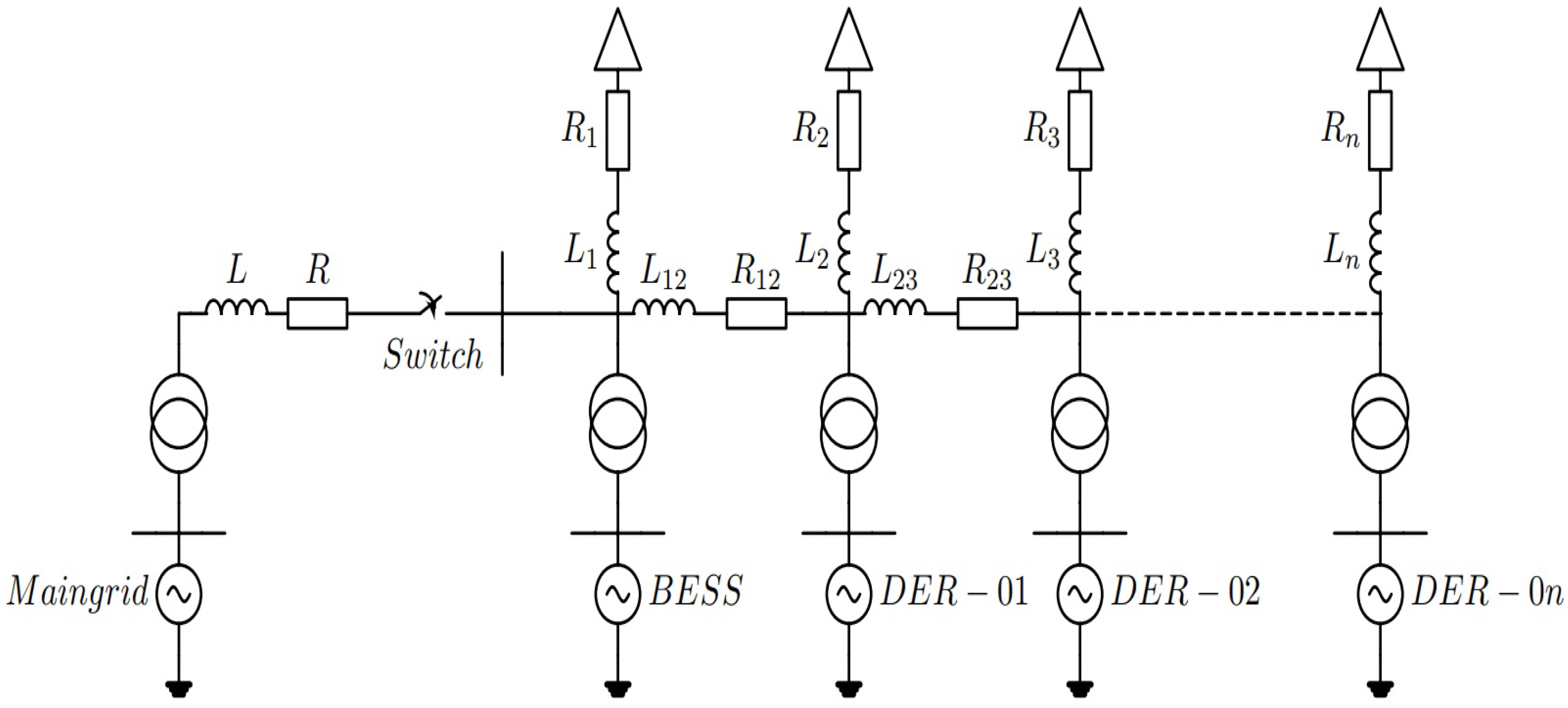
Figure 2. Schematic block diagram of a PV system.

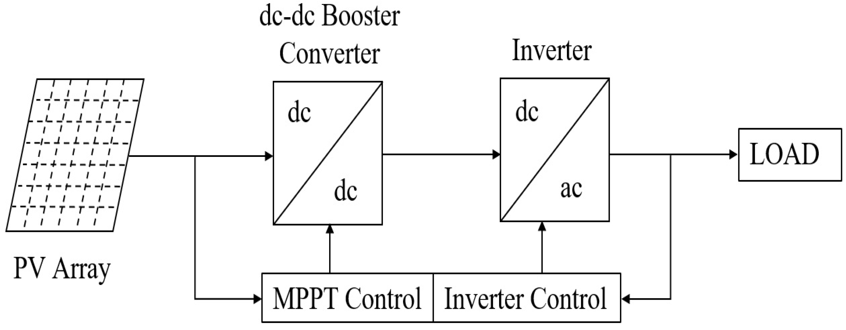
Figure 3. Schematic block diagram of a PV system.

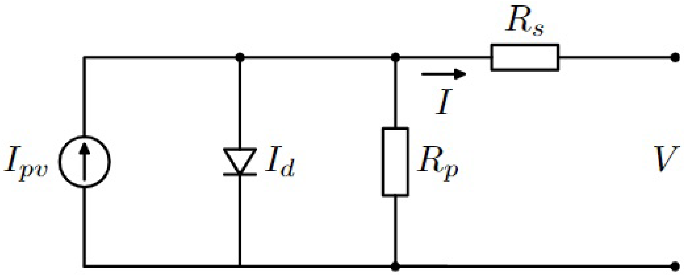
Figure 4. Reserve power in de-loaded PV system.

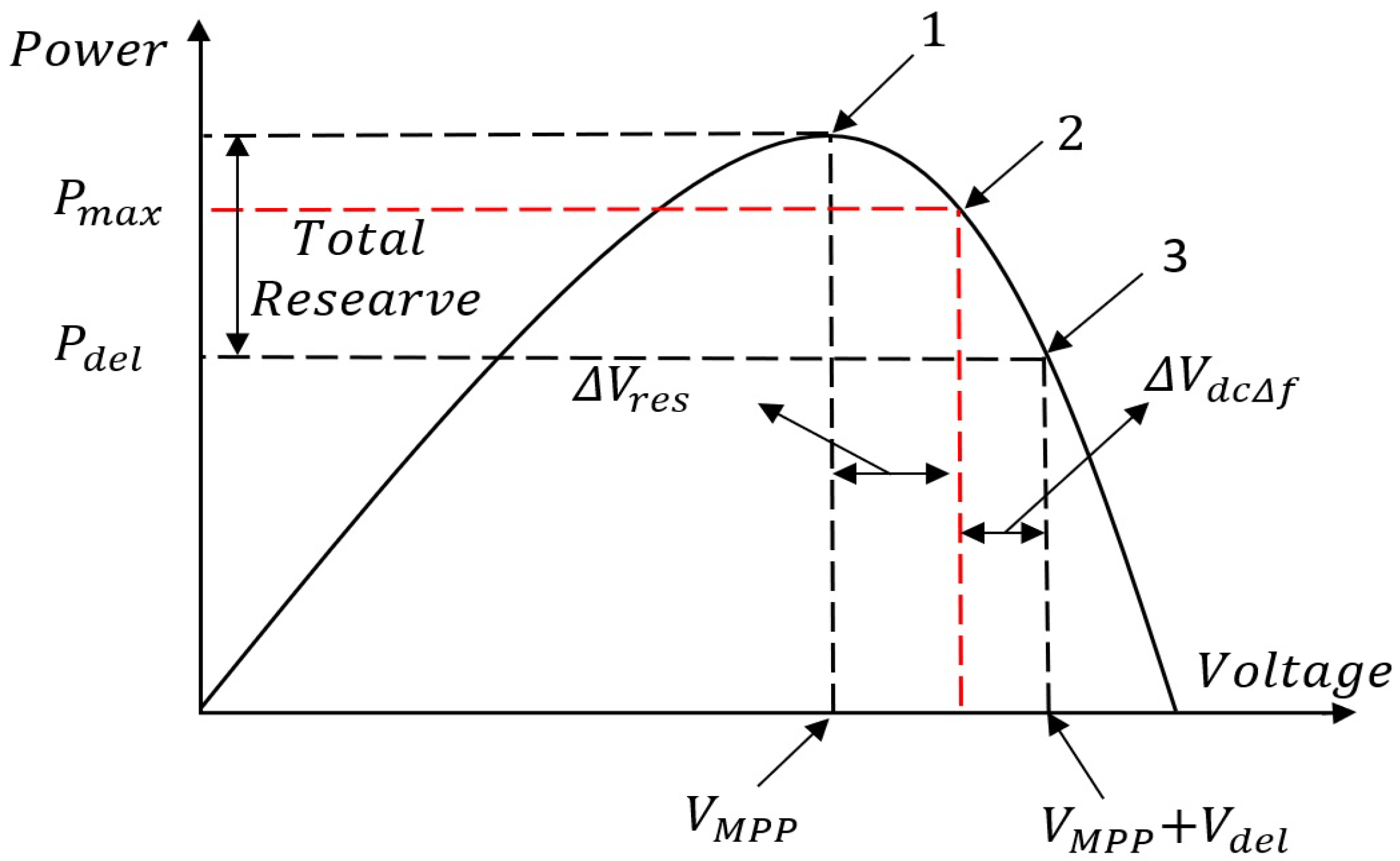
Figure 5. Controller for de-loaded solar PV[32].

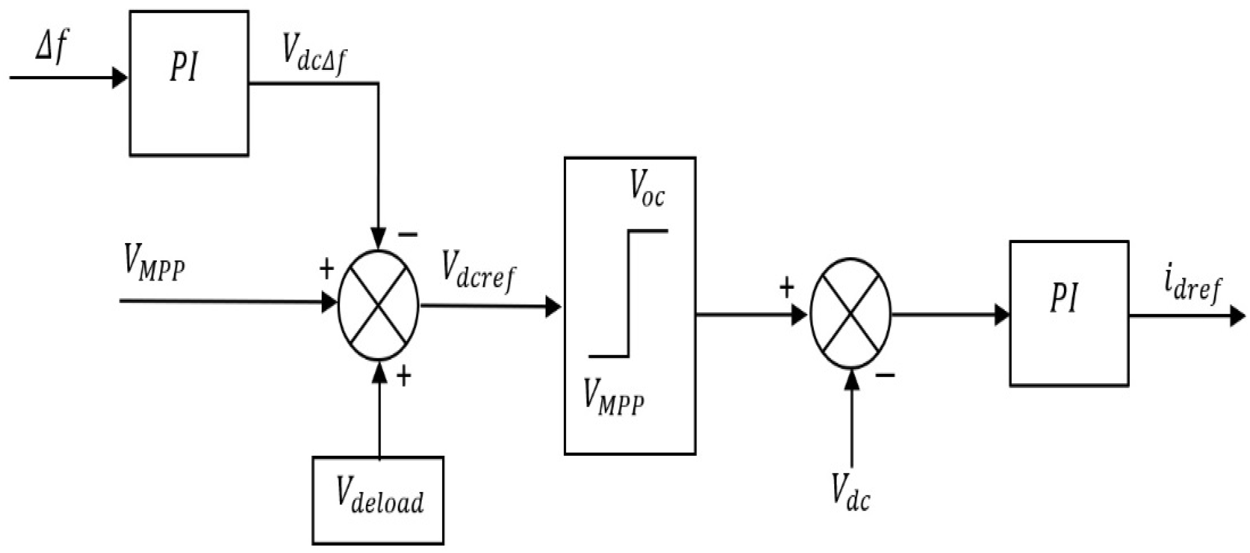
Figure 6. Schematic diagram of a wind generation system with the DFIG[25].

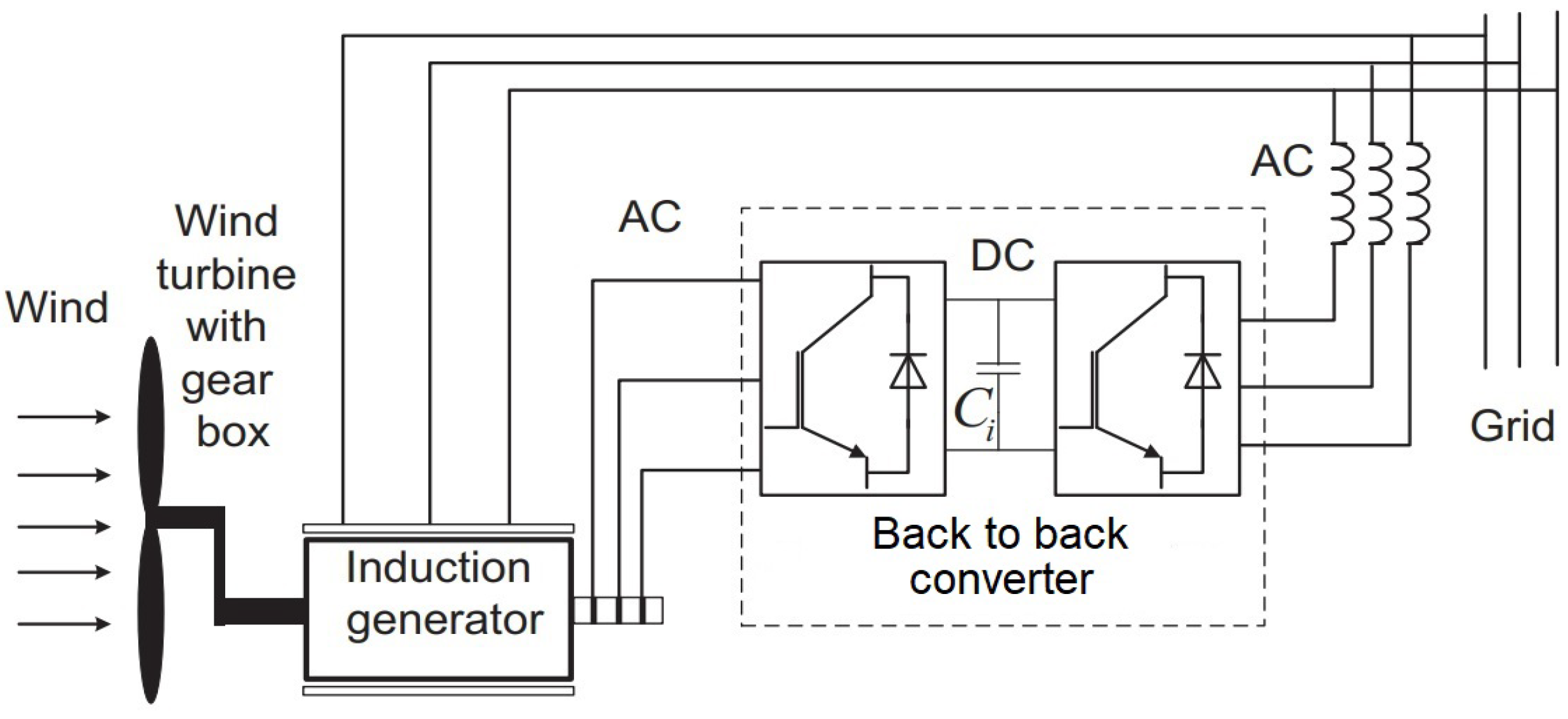
Figure 7. Power rotor-speed curves for different values of pitch angle for a 1.5 MW wind turbine (wind speed: 10 m/s)[33].

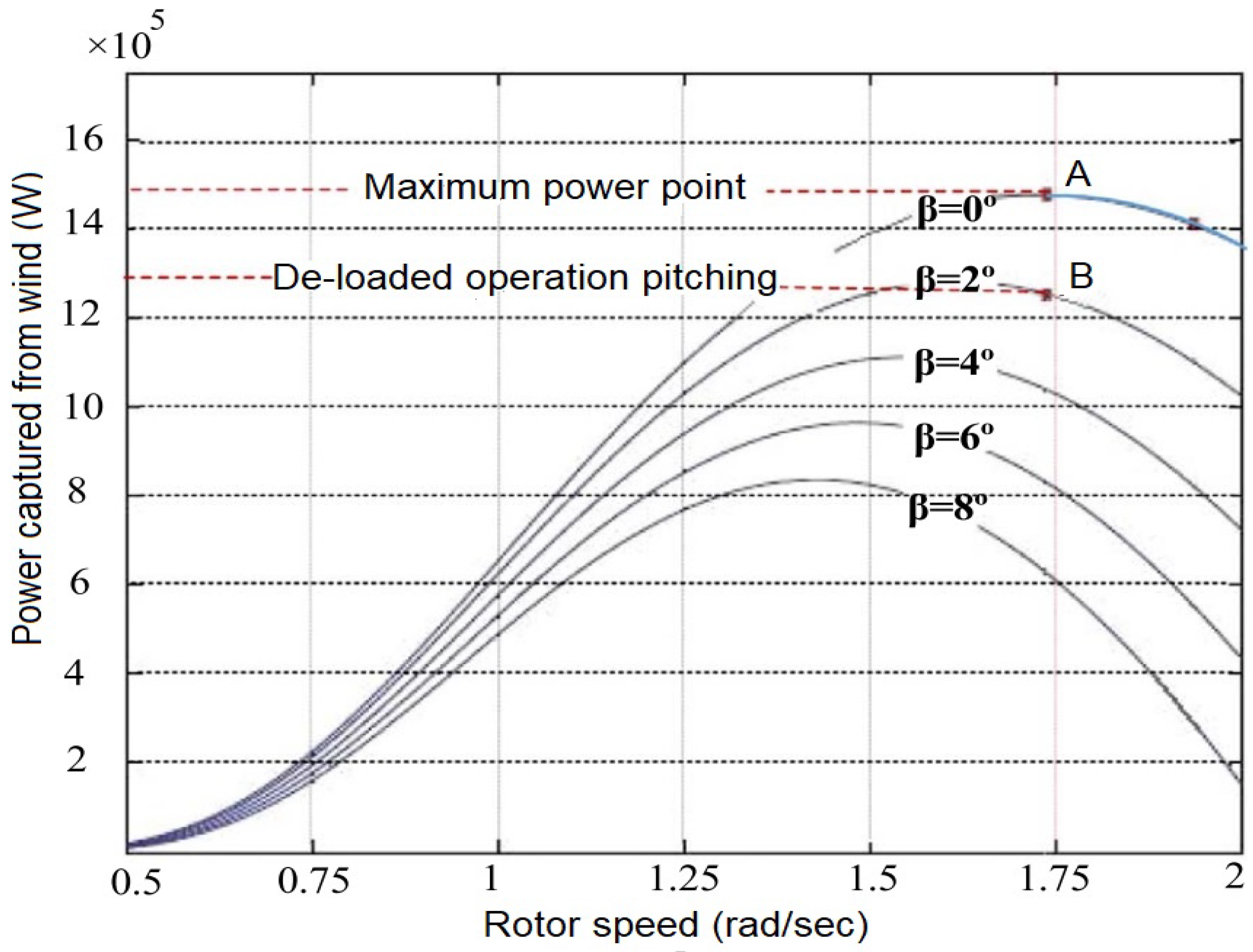
Figure 8. PLL block diagram.

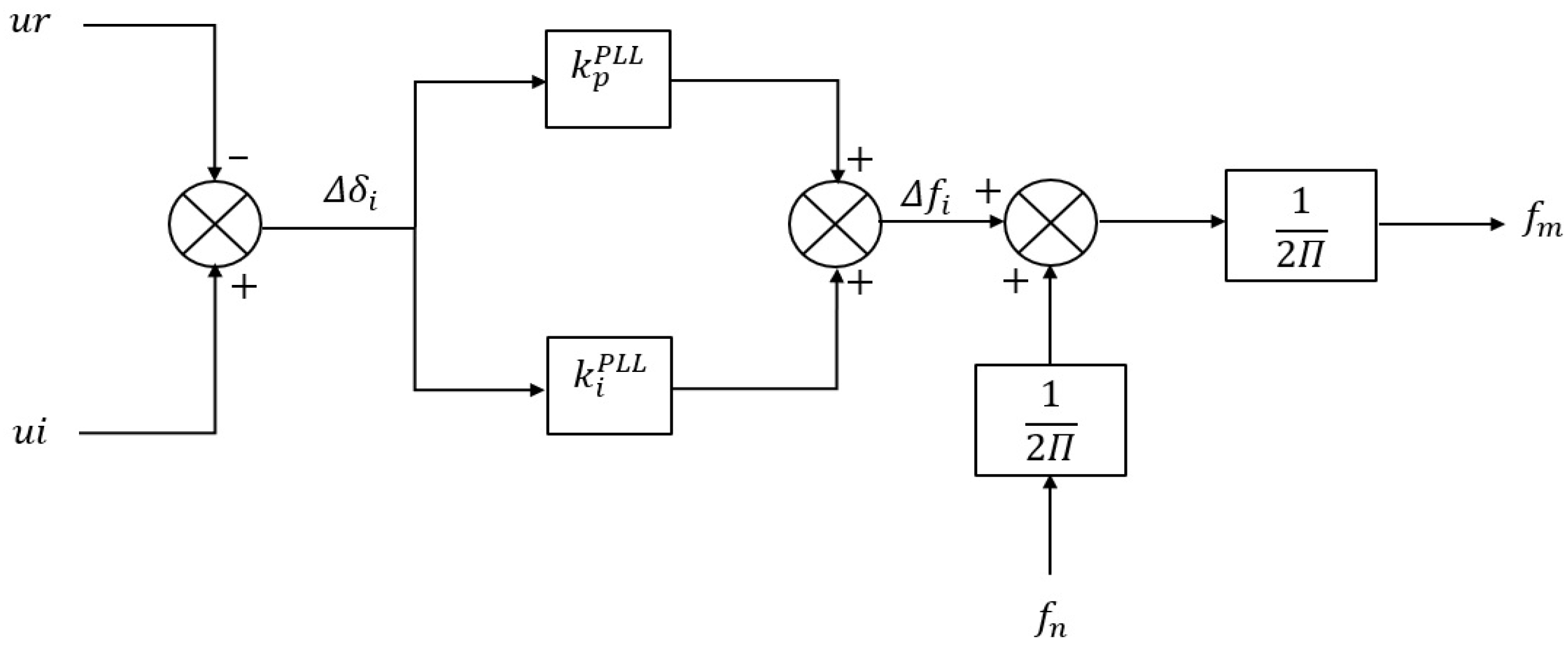
Figure 9. Control structure of grid forming VSI for active power sharing.

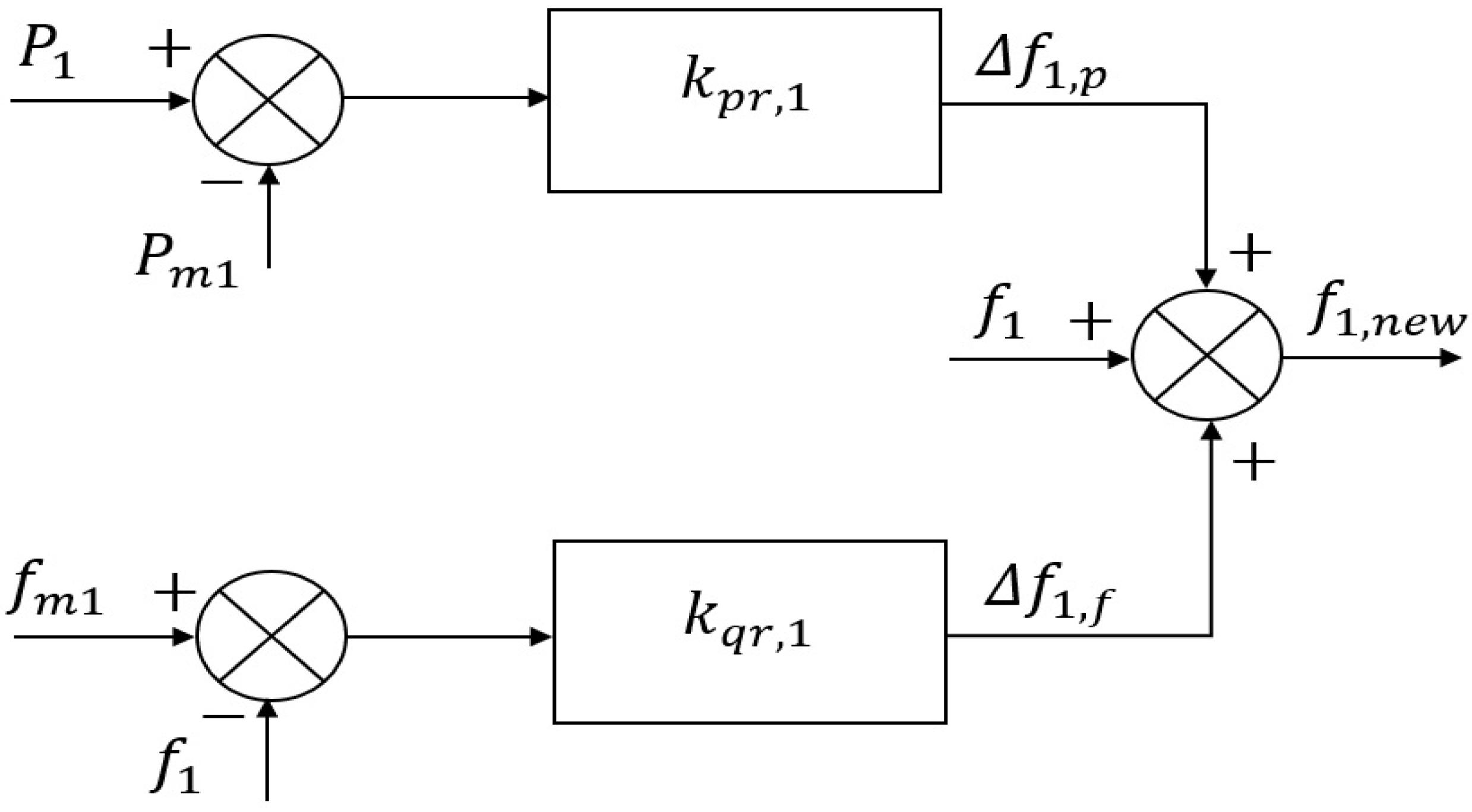
Figure 10. Control structure for grid following inverters for active power sharing.

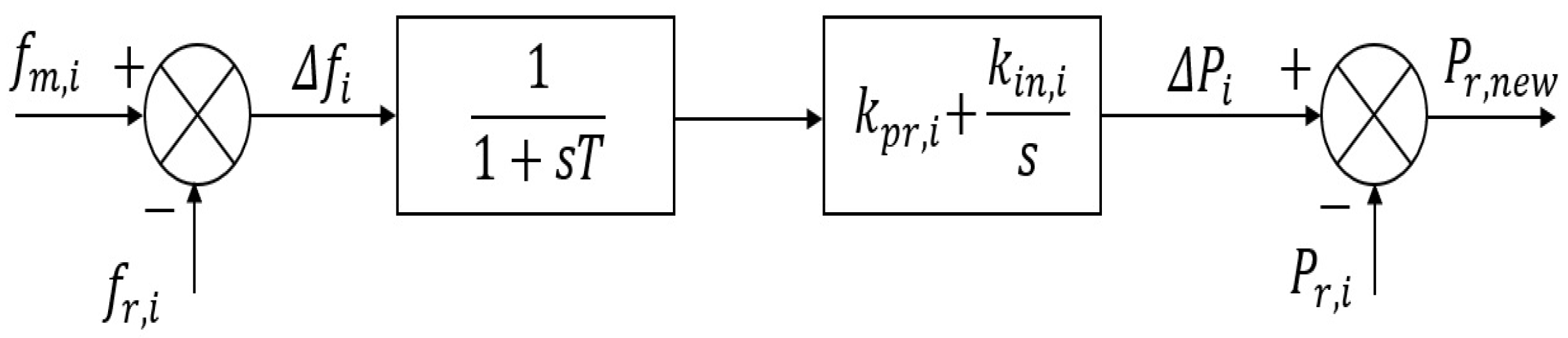
Figure 11. Poles and zeroes map.

Figure 12. Block diagram of transfer function.

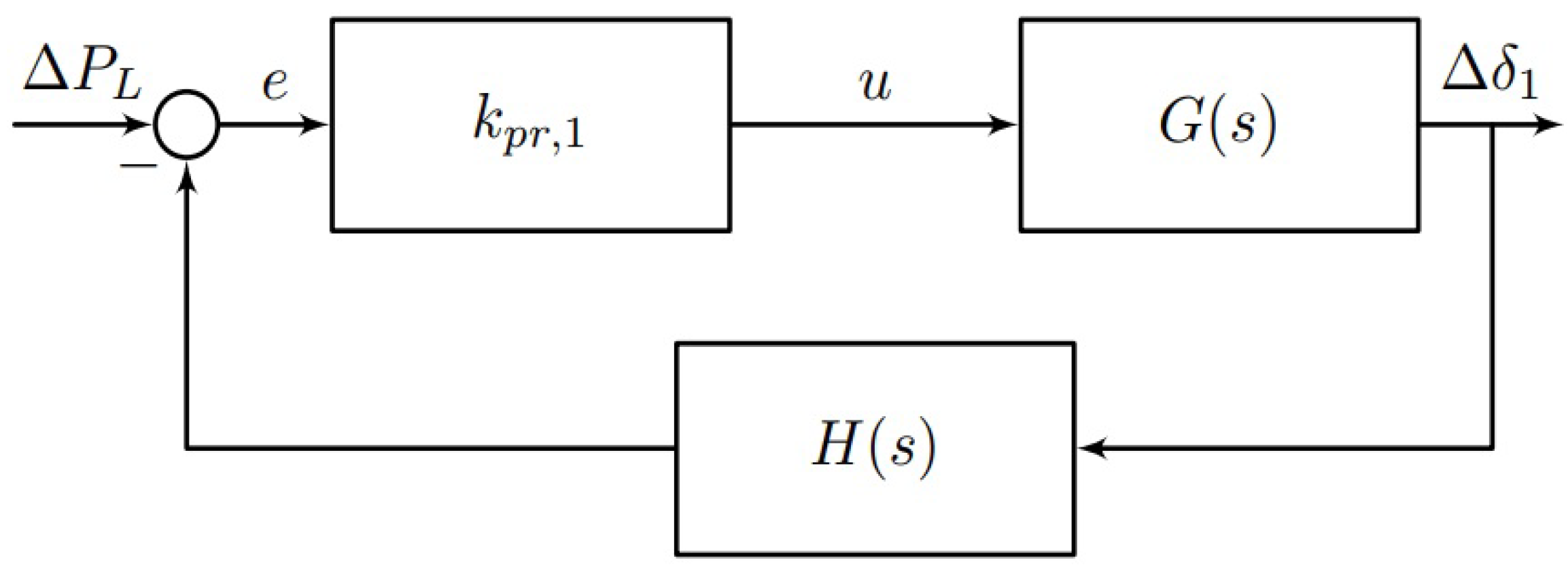
Figure 13. Root locus.

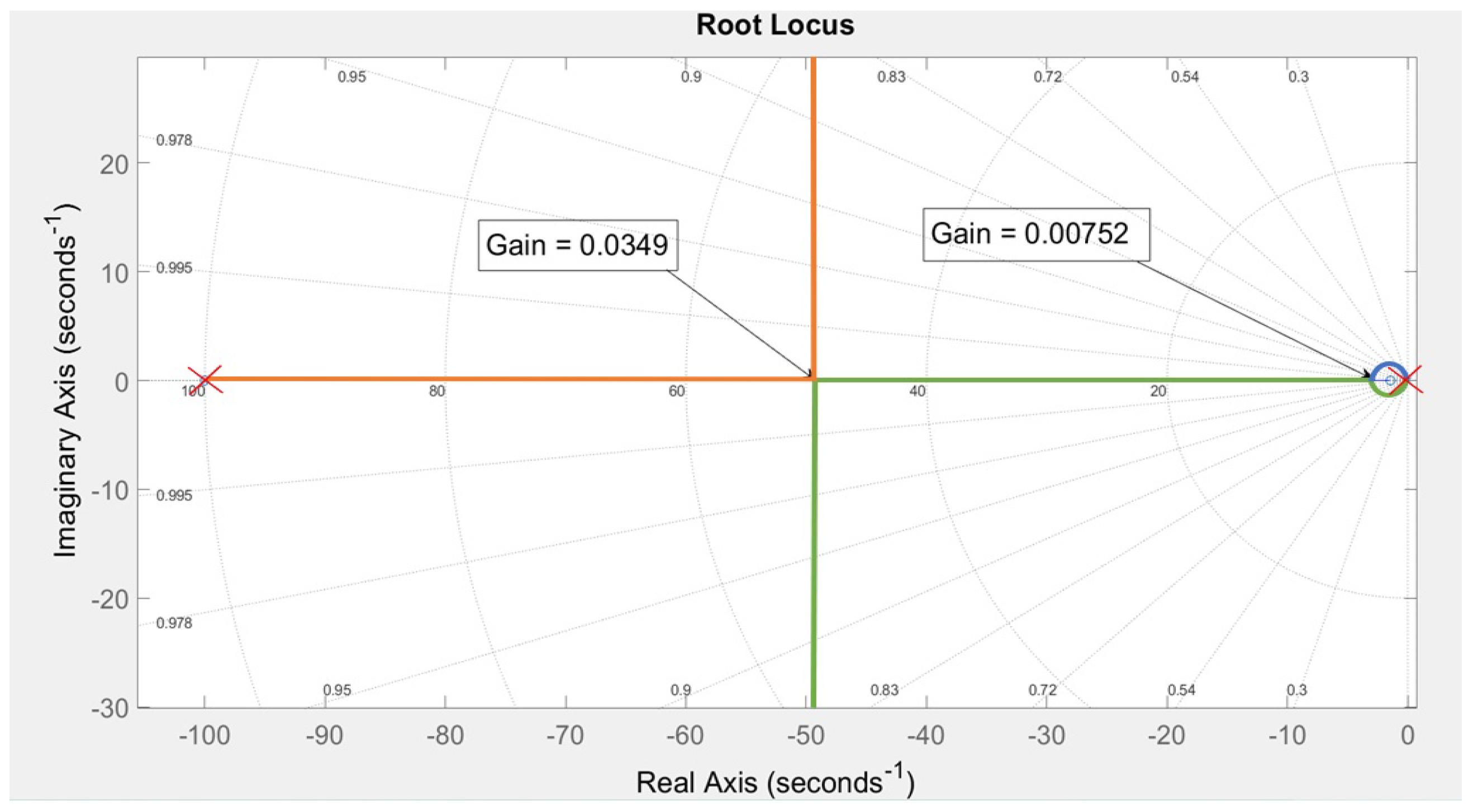
Figure 14. Frequency change with load change events.

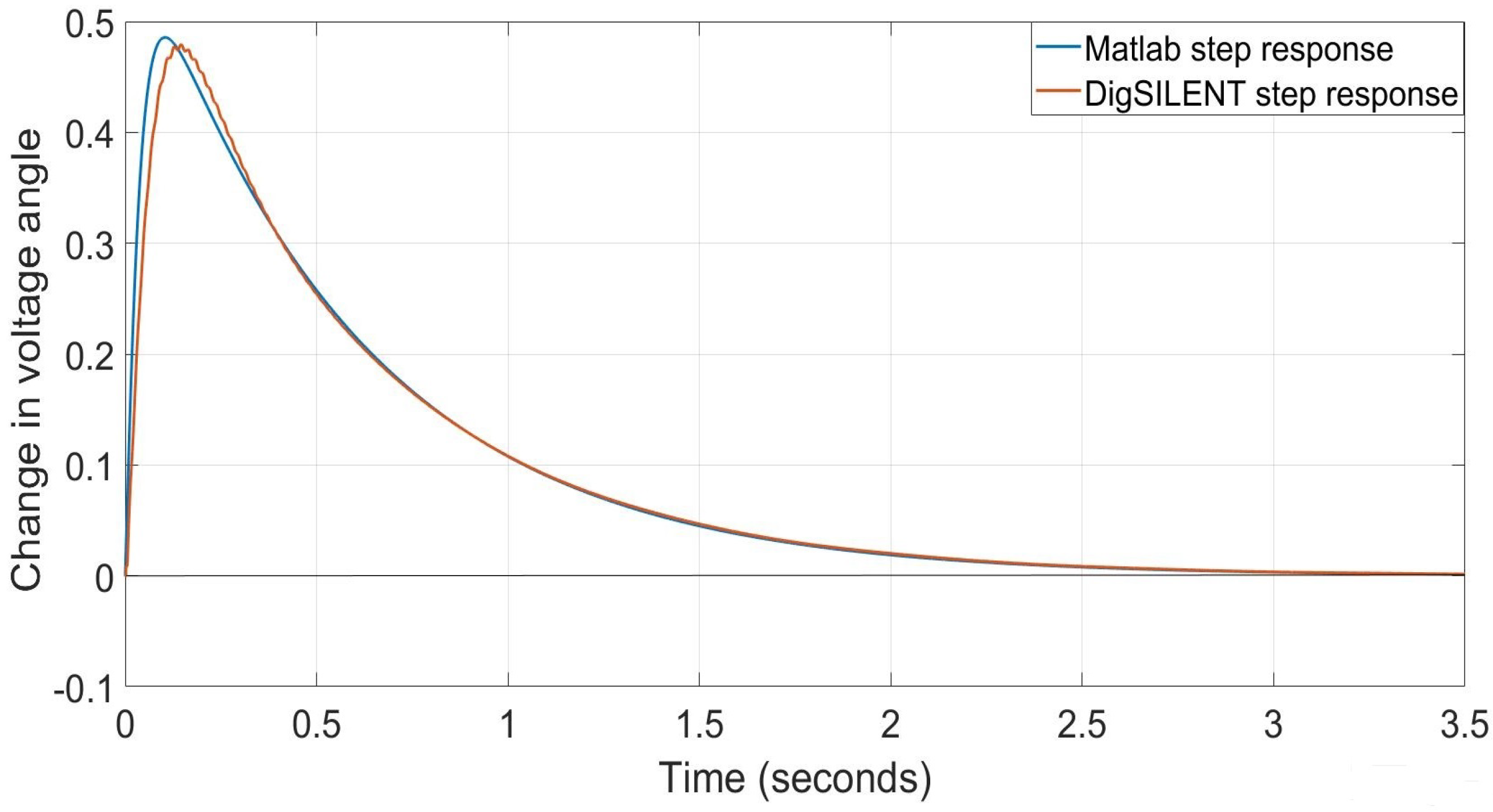
Figure 15. Step response for total changes in active power and power angle/ frequency by DER units.

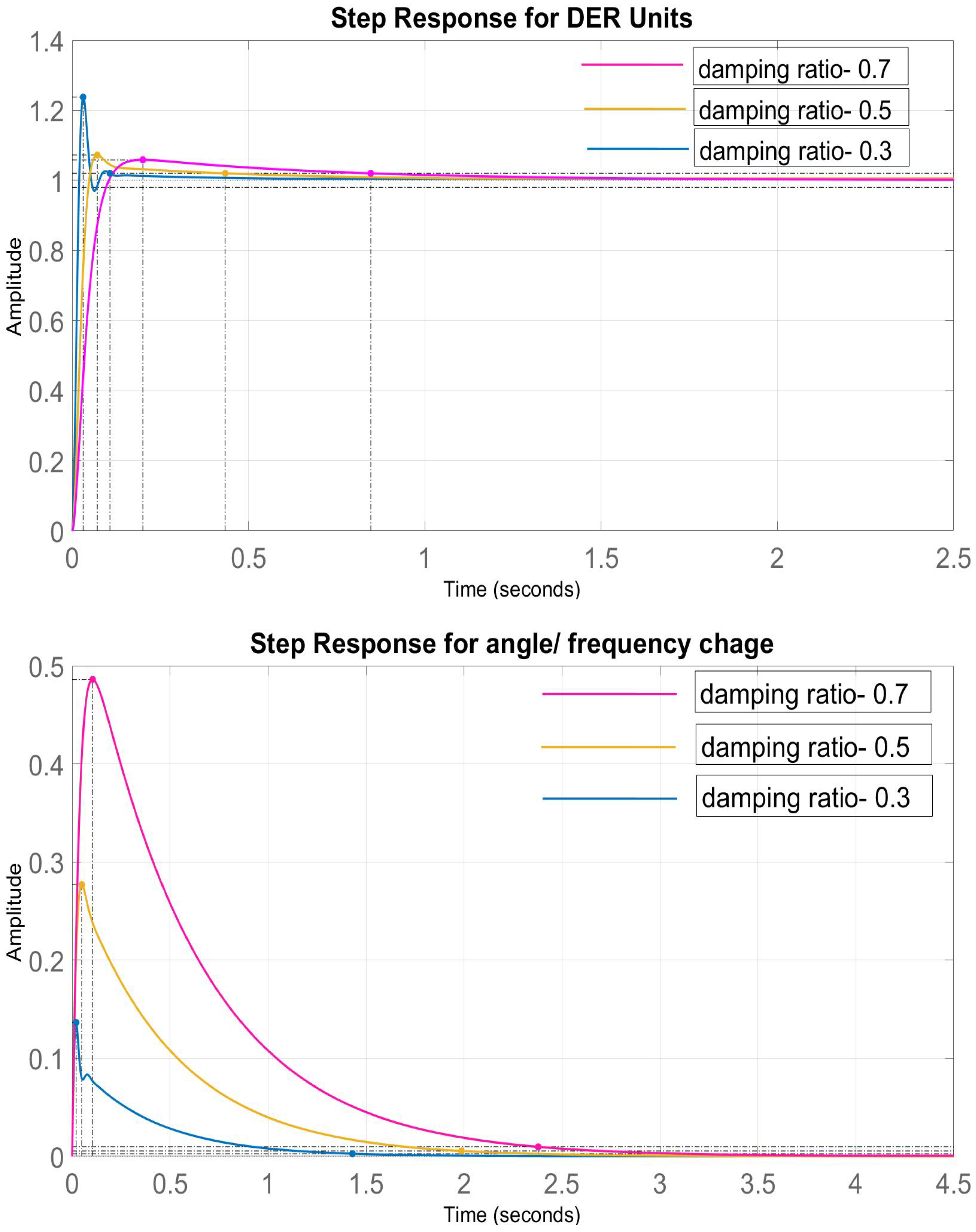
Figure 16. Trajectory of performance index (PSO-PID4).

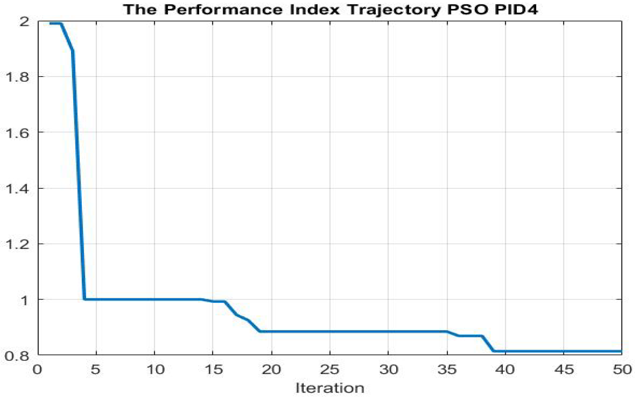
Figure 17. Parameter values.

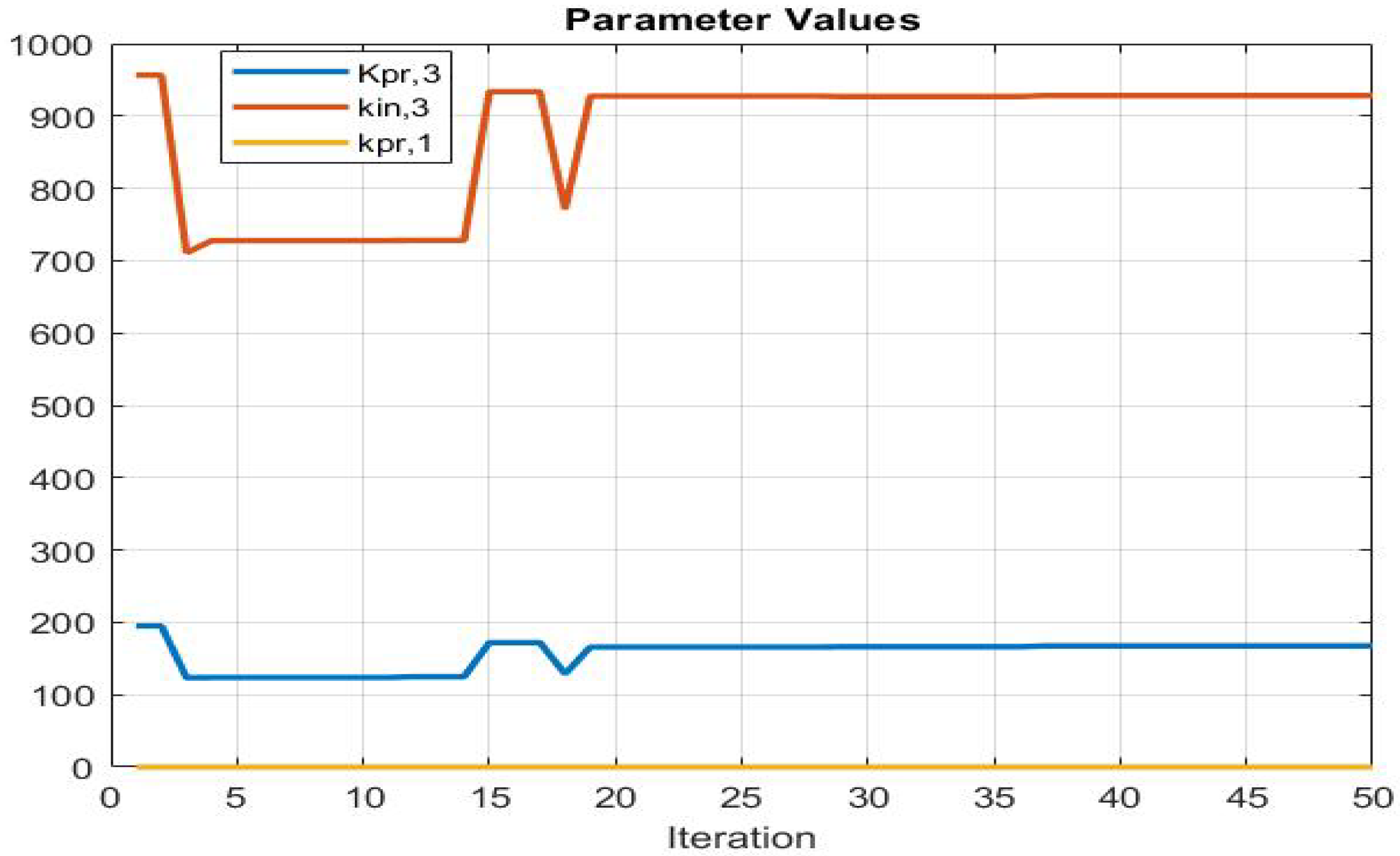
Figure 18. Comparison of step responses of PI controllers for active power changes.

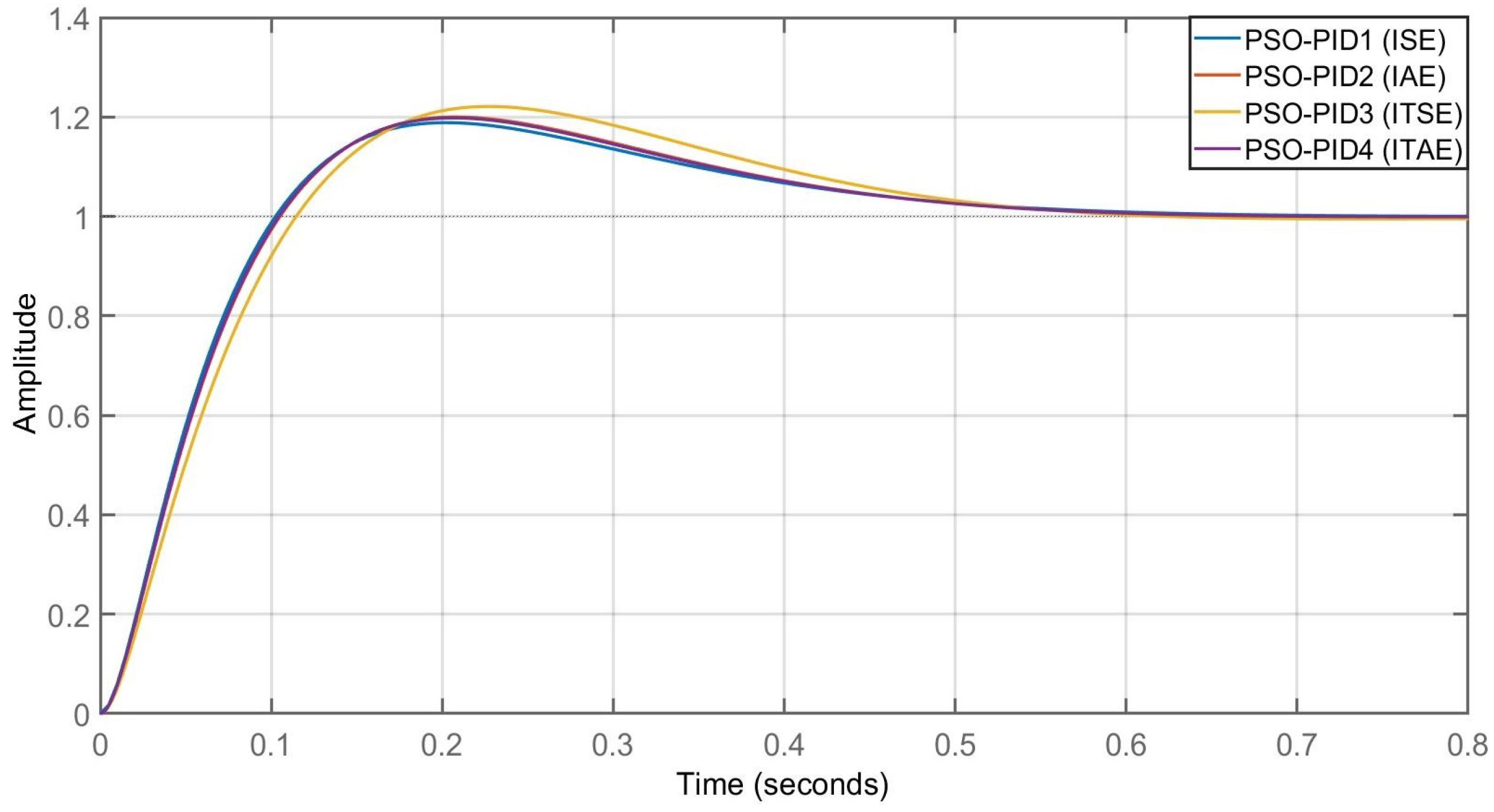
Figure 19. Comparison of step responses of PI controllers for frequency changes.

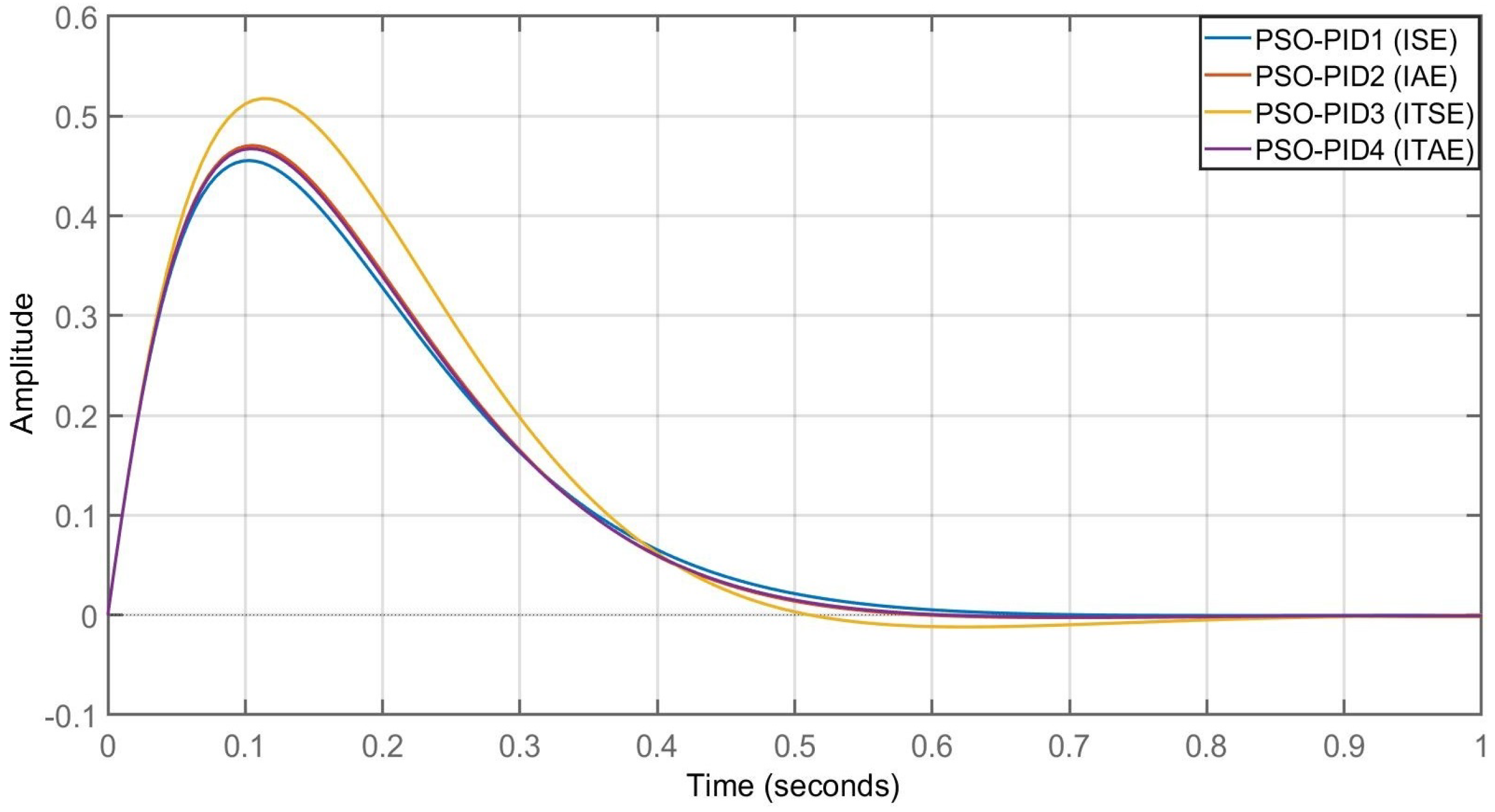
Figure 20. Comparison of step responses of of frequency changes using Ziegler-Nichols and PSO methods.

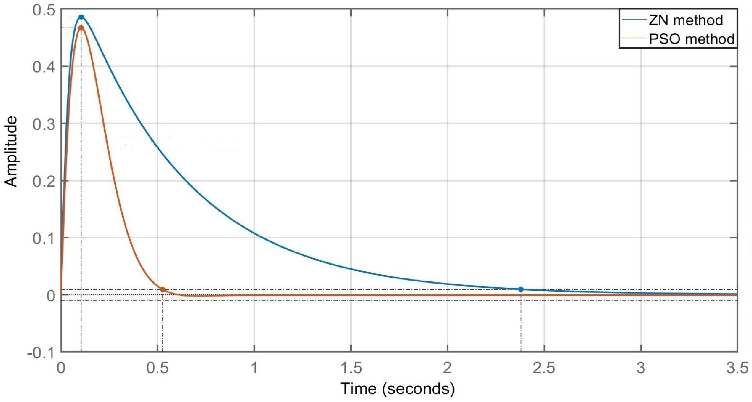
Figure 21. Comparison of step responses of active power changes using Ziegler-Nichols and PSO methods.

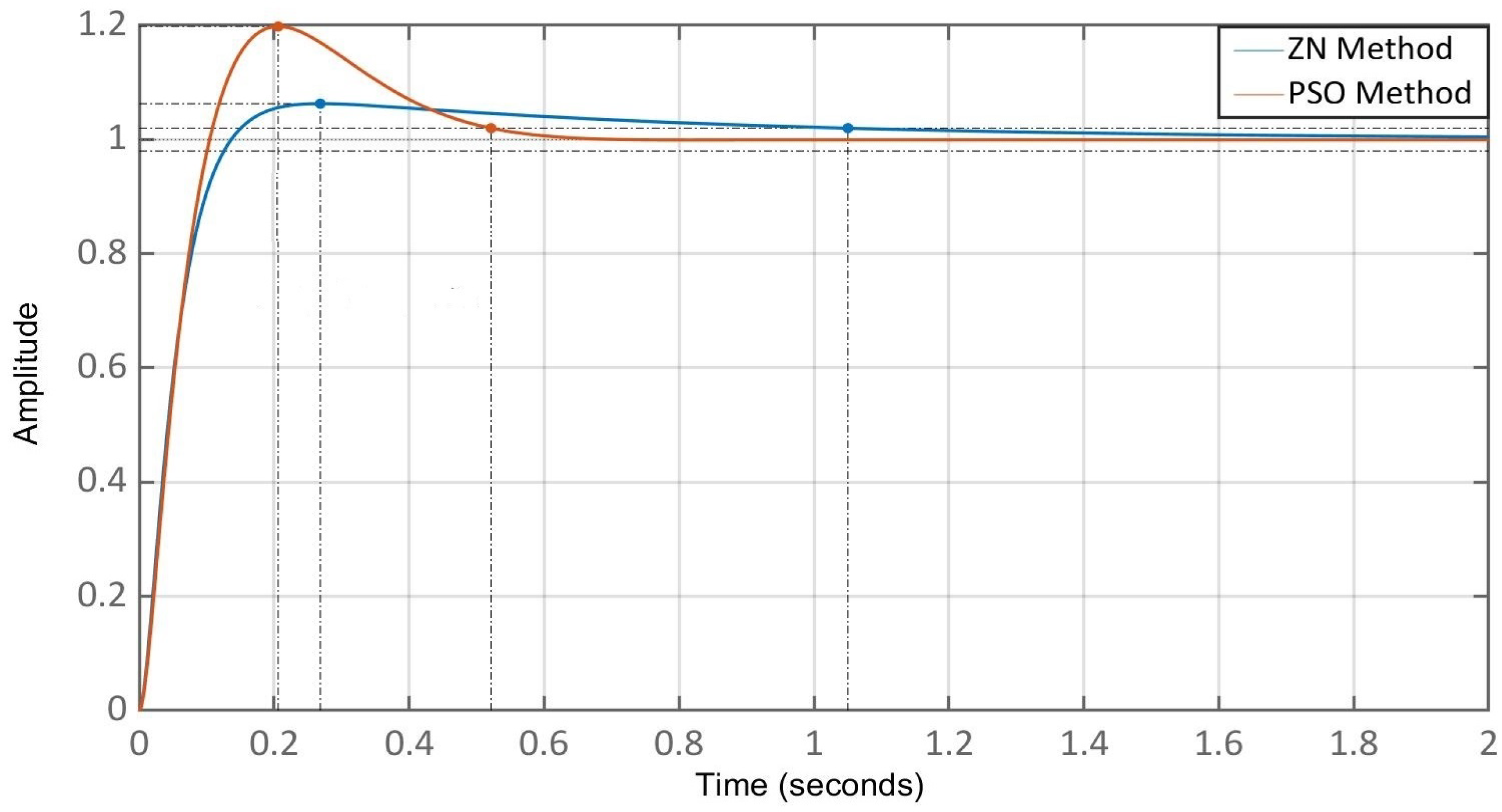
Figure 22. General model of the network.

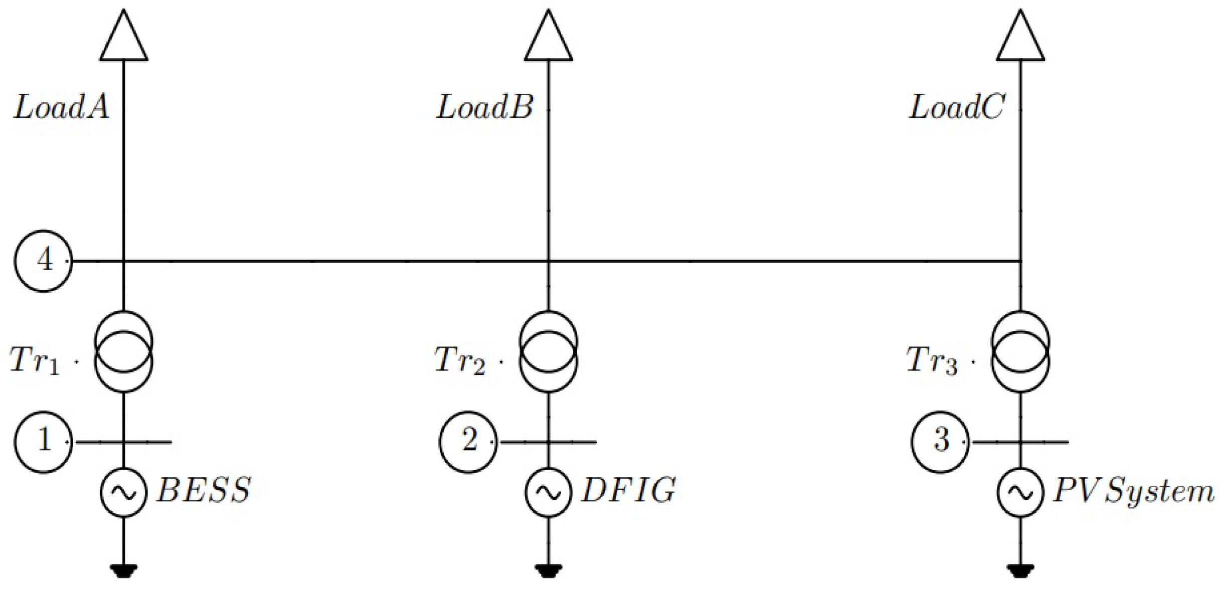
Figure 23. Active power-sharing by DER units (wind generator, BESS and PV system) for L-type 4-bus network.

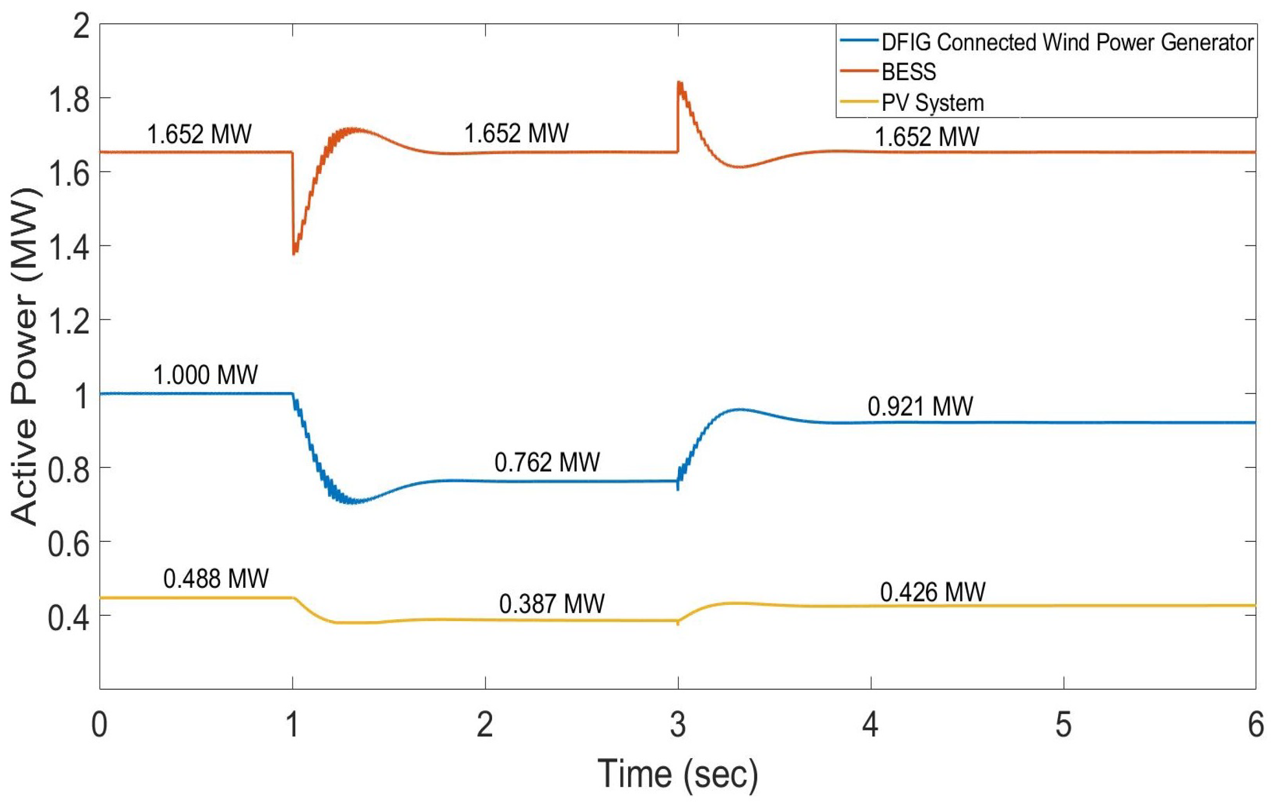
Figure 24. Frequency changes in network for active load change.

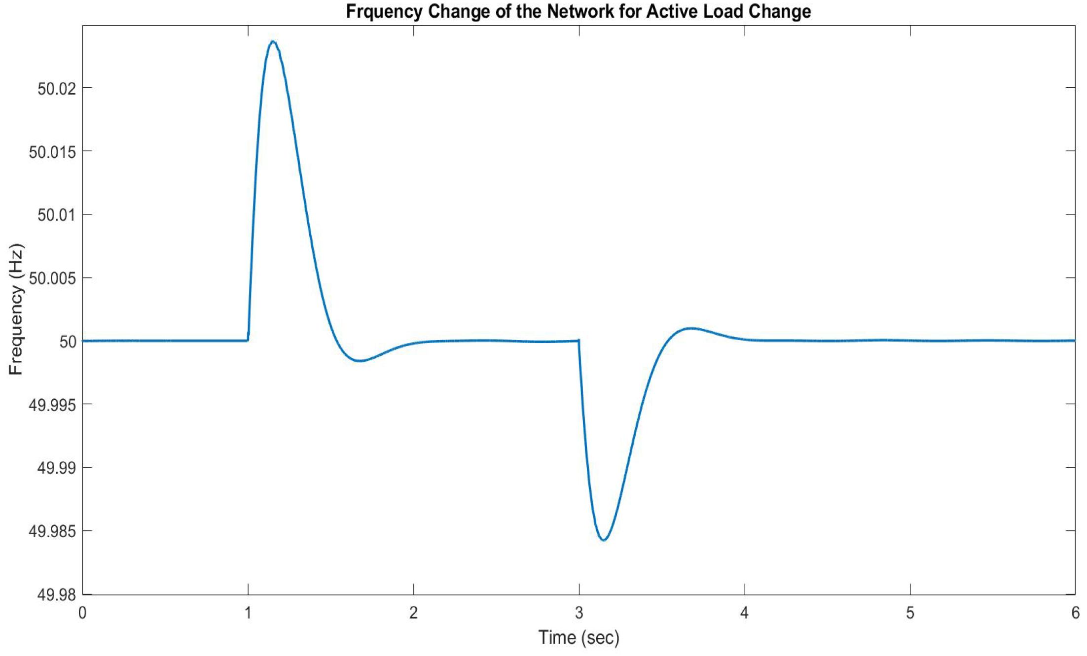
Figure 25. 9-Bus Grid

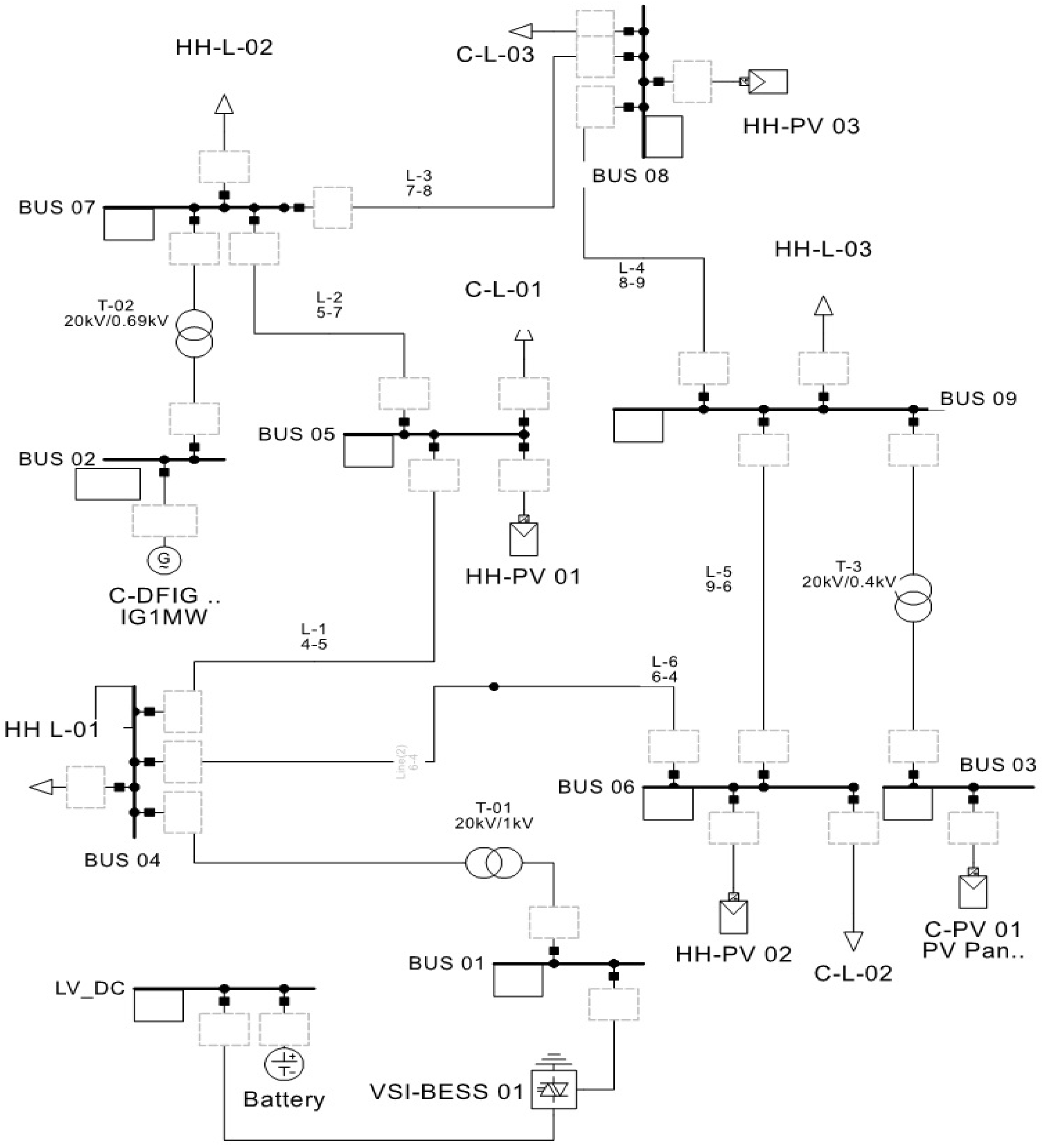
Figure 26. Active power-sharing by DER units (wind generator, BESS and PV system) for RL-type 9-bus network.

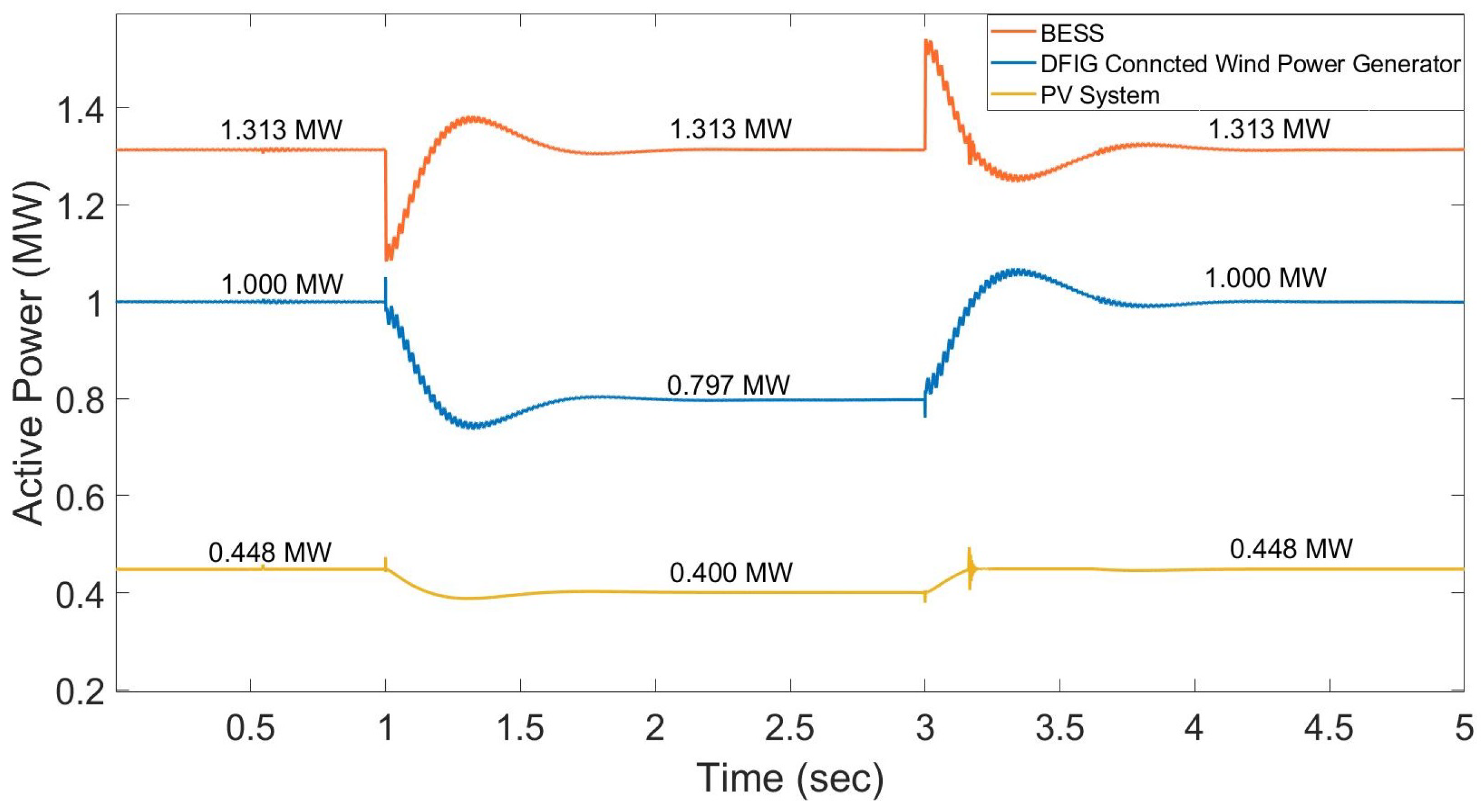
Figure 27. Frequency of network while sharing active power- RL-type 9 bus.

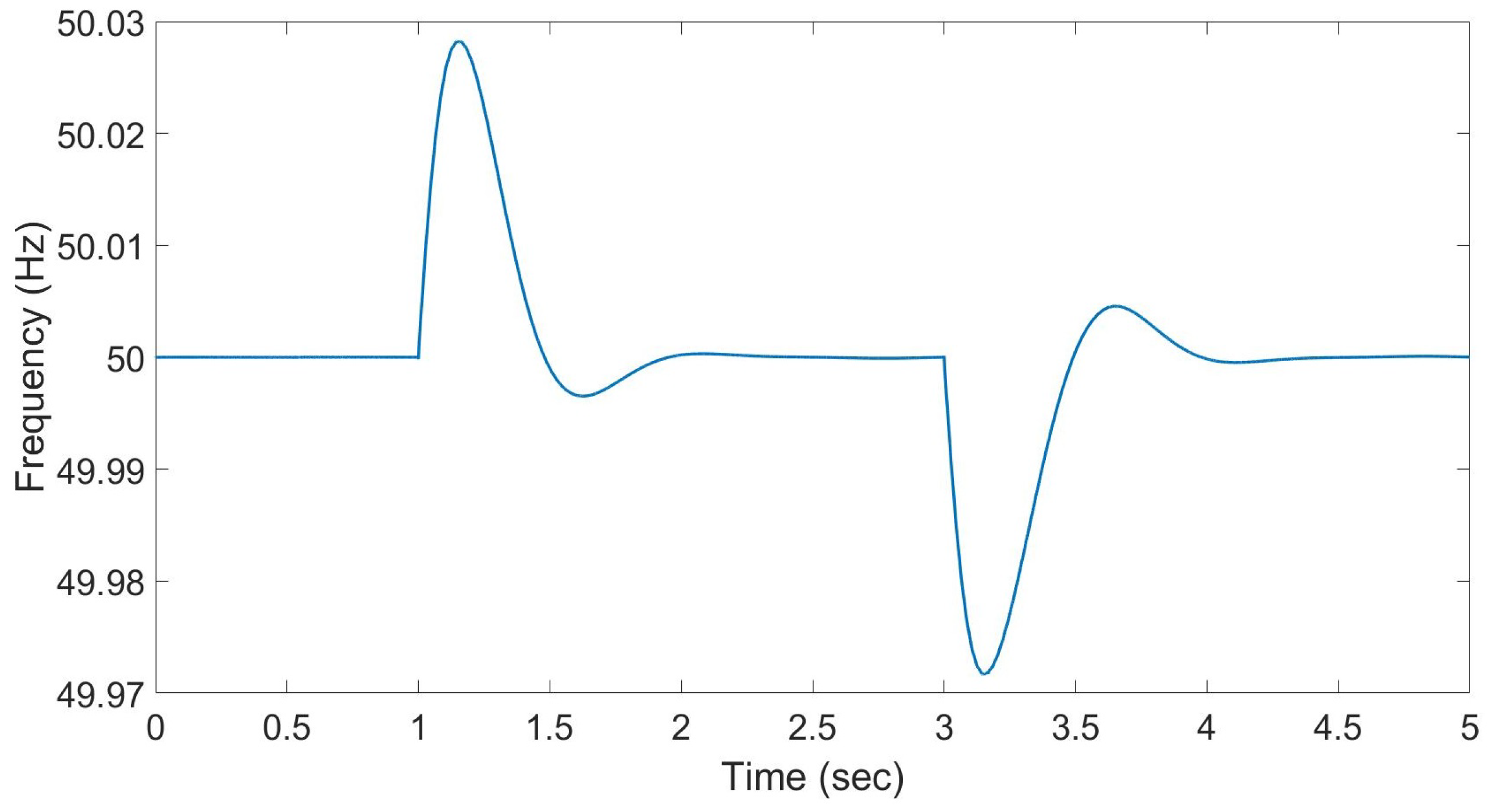
Figure 28. Active power-sharing by household DER units (wind generator, BESS and PV system) for RL-type 9-bus network.

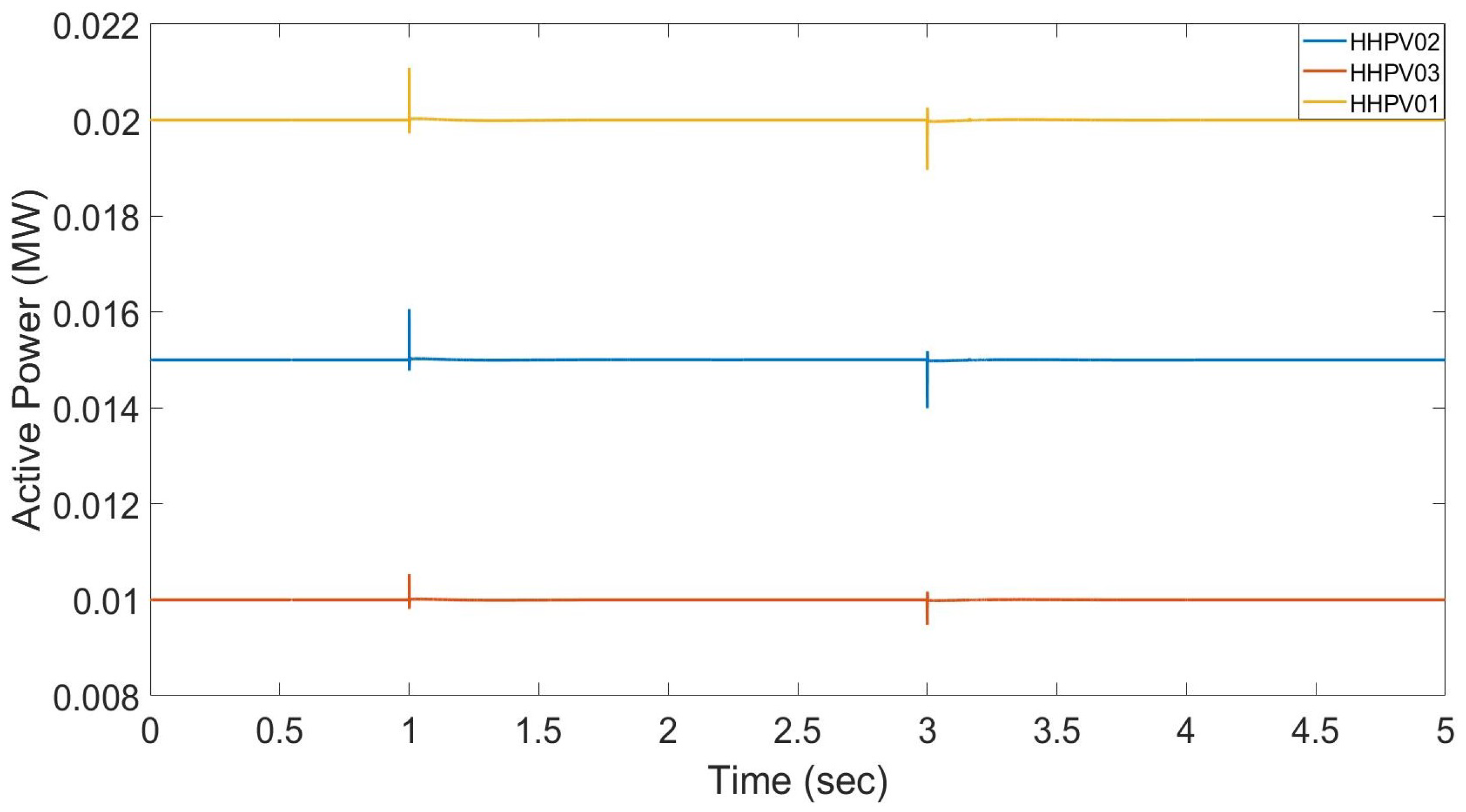
Figure 29. Active power-sharing by DER units (wind generator, BESS (in ‘sharing’ mode) and PV system) for L-type 4-bus network.

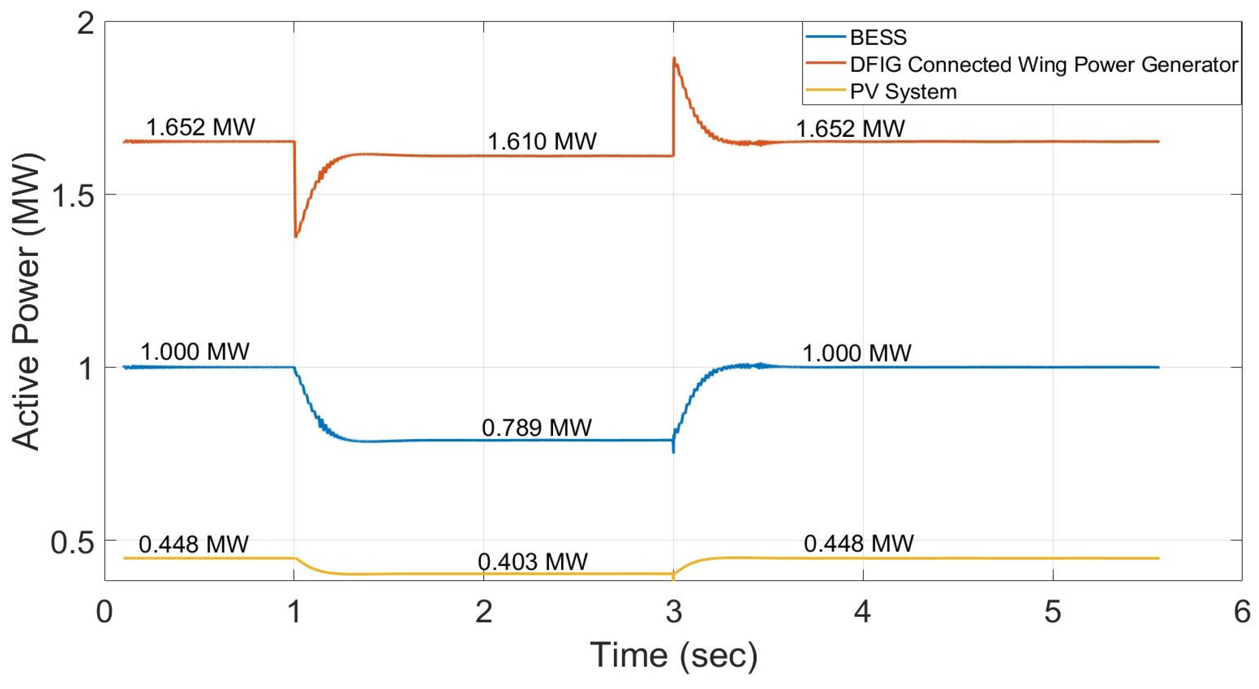
Table 1. Ziegler-Nichols closed-loop tuning parameter.

Control Type	$K_{P}$	$K_{I}$
PI	0.45 $K_{u}$	0.45 $K_{u} / T_{u}$

Table 2. Calculated control tuning parameters as per Ziegler-Nichols method.

Value of $ξ$	$K_{u}$	$T_{u}$	$k_{p r, 2}$	$k_{i n, 2}$	$k_{p r, 3}$	$k_{i n, 3}$
0.3	2369.7	0.4867	2132.7	5258.4	1066.4	2629.2
0.5	853.08	0.6283	767.78	1466.3	383.89	733.17
0.7	435.25	0.7434	391.72	632.29	195.86	316.14

Table 3. Optimized PI parameters for 4-bus L type network.

Tuning method	$k_{p r, 1}$	$k_{p r, 2}$	$k_{i n, 2}$	$k_{p r, 3}$	$k_{i n, 3}$
ZN method	0.0243	571	952	285	475
PSO-PID1 (ISE)	0.0312	355	1860	167	930
PSO-PID2 (IAE)	0.0312	331	1848	165	924
PSO-PID3 (ITSE)	0.0312	289	1690	144	845
PSO-PID4 (ITAE)	0.0312	334	1856	167	928

Table 4. Optimized PI parameters for 9-bus L type network.

Tuning method	$k_{p r, 1}$	$k_{p r, 2}$	$k_{i n, 2}$	$k_{p r, 3}$	$k_{i n, 3}$
ZN method	0.0243	571	952	285	475
PSO-PID1 (ISE)	0.01	485	1536	242	768
PSO-PID2 (IAE)	0.0539	277	1553	138	776
PSO-PID3 (ITSE)	0.0539	458	1536	229	768
PSO-PID4 (ITAE)	0.0539	222	1465	111	732

Table 5. Line parameters of L-type 4 bus network.

Node From	Node To	Resistance, (p.u.)	Reactance, (p.u.)
1	4	0	4.0
2	4	0	4.0
3	4	0	1.5

Table 6. Initial values of DFIG, PV system, BESS and loads L-type 4 bus system.

Element Name	Bus Type	Real Power ( $P^{0}$ ) MW	Reactive Power ( $Q^{0}$ ) MVar	Voltage ( $V^{0}$ ) kV	Voltage Angle( $δ^{0}$ )
VSI-BESS 01	Slack	-	-	1.0	0 $^{\circ}$
DFIG-Wind Gen.	PV	1.00	-	0.69	-
PV System	PV	0.448	-	0.4	-
Load A	PQ	2.8	0.0	20.0	-
Load B	PQ	0.3	0.0	20.0	-
Load C	PQ	0.2	0.0	20.0	-

Table 7. Initial values of known and unknown variables after load flow analysis- L-type 4 bus system.

Bus no	Voltage (p.u).	Voltage Angle $δ^{0} deg$	Real Injected Power $P^{0}$ (MW)	Reactive Injected Power $Q^{0}$ (MVAR)
1	1.0000	0.0	1.652	0.046
2	1.0000	0.8728	1.000	0.030
3	1.0000	-0.3933	0.448	0.006
4	0.9996	-1.4205	-3.1	0.0

Table 8. RL-type 9-bus system.

System name	Co-efficient	Value
BESS	$k_{p r, 1}$	0.0312
Wind generator	$k_{p r, 1}$	334.88
Wind generator	$k_{i n, 1}$	1856.54
PV System	$k_{p r, 2}$	167.44
PV System	$k_{i n, 2}$	928.27

Table 9. Initial values of DFIG, PV system, BESS and loads.

Element Name	Bus Type	Real Power ( $P^{0}$ ) MW	Reactive Power ( $Q^{0}$ ) MVar	Voltage ( $V^{0}$ ) kV	Voltage Angle( $δ^{0}$ )
C-DFIG 01	PV	1.00	-	0.69	-
C-PV 01	PV	0.448	-	0.4	-
VSI-BESS 01	Slack	-	-	1.0	0 $^{\circ}$
HH-PV 01	PQ	0.02	0.0	20.0	-
HH-PV 02	PQ	0.015	0.0	20.0	-
HH-PV 03	PQ	0.01	0.0	20.0	-
HH-L-01	PQ	0.01	0.0	20.0	-
HH-L-02	PQ	0.018	0.0	20.0	-
HH-L-03	PQ	0.025	0.0	20.0	-
C-L-01	PQ	1.7	0.0	20.0	-
C-L-02	PQ	0.25	0.0	20.0	-
C-L-03	PQ	0.8	0.0	20.0	-

Table 10. Parameters of the 9 bus network.

Node From	Node From	Resistance, $(p . u .)$	Reactance, $(p . u .)$
1	4	0	2.0
2	7	0	1.5
3	9	0	3.0
4	5	0.14475	0.09175
4	6	0.072375	0.045875
5	7	0.217125	0.137625
6	9	0.188175	0.119275
7	8	0.2316	0.1468
8	9	0.26055	0.16515

Table 11. All the initial values of known and unknown variables after load flow analysis.

Bus no	Voltage (p.u).	Voltage Angle $δ^{0} deg$	Real Injected Power $P^{0}$ (MW)	Reactive Injected Power $Q^{0}$ (MVAR)
1	1.0000	0.0	1.313	0.015
2	1.0000	-0.3678	1.000	0.027
3	1.0000	–3623	0.448	0.012
4	0.9998	-1.2224	-0.01	0.0
5	0.9946	-1.4122	-1.68	0.0
6	0.9997	-1.2267	-0.235	0.0
7	0.9998	-1.2275	-0.018	0.0
8	0.9988	-1.2601	-0.79	0.0
9	0.9999	-1.2219	-0.025	0.0

Table 12. Values of controller co-coefficients-RL-type 9 bus.

System name	Co-efficient name	Value
BESS	$k_{p r, 1}$	0.0243
Wind generator	$k_{p r, 1}$	222.68
Wind generator	$k_{i n, 1}$	1465.13
PV System	$k_{p r, 2}$	111.34
PV System	$k_{i n, 2}$	732.56

Disclaimer/Publisher’s Note: The statements, opinions and data contained in all publications are solely those of the individual author(s) and contributor(s) and not of MDPI and/or the editor(s). MDPI and/or the editor(s) disclaim responsibility for any injury to people or property resulting from any ideas, methods, instructions or products referred to in the content.

© 2024 by the authors. Licensee MDPI, Basel, Switzerland. This article is an open access article distributed under the terms and conditions of the Creative Commons Attribution (CC BY) license (http://creativecommons.org/licenses/by/4.0/).

Copyright: This open access article is published under a Creative Commons CC BY 4.0 license, which permit the free download, distribution, and reuse, provided that the author and preprint are cited in any reuse.

Downloads

118

Views

Comments

Subscription

Notify me about updates to this article or when a peer-reviewed version is published.

MDPI Initiatives

Important Links

Choose an area of interest and we will send you notifications of new preprints at your preferred frequency.

Disclaimer

A Systematic Approach to Designing Power Sharing Control of Converter-Based Generators

Abstract

Keywords:

Subject:

1. Introduction

2. System overview

2.1. BESS Model

2.2. DER Model

2.2.1. PV System

2.2.2. DFIG-connected Wind Power Generator

2.3. PLL

2.4. Observations

3. Proposed power sharing

3.1. BESS

3.2. DER units

4. Linearised model and gain selection

4.1. Linearised model

4.2. Gain selection

4.2.1. Ziegler-Nichols Method

4.2.2. PSO algorithm

5. Simulation results

5.1. L-type 4-bus system

5.2. RL-type 9-bus system

5.3. Power-sharing mode of BESS controller

6. Conclusion

Abbreviations

References

MDPI Initiatives

Important Links

Subscribe