
Submitted:
09 January 2024
Posted:
11 January 2024
You are already at the latest version
Abstract
Solar energy adoption worldwide has expanded exponentially due to a surge in international interest in producing clean energy and the declining cost of solar power plants and their technology. It is anticipated that by 2050, solar will have surpassed fossil fuels to become the primary source of energy. However, one of the main challenges associated with solar energy production is the instability of photovoltaic (PV) power generation because of weather changes. Short-term forecasting of the power output of photovoltaic systems is essential for efficient management of the power grid and energy markets. This paper aims to evaluate the ability of deep learning (DL) models to provide accurate forecasting of hourly global horizontal irradiance (GHI) using different sets of features, including weather and aerosol variables along with solar radiation components. The results show that the best forecast skills are achieved by the long short-term memory autoencoder (LSTM-AE) model.
Keywords:
GHI forecasting
; deep learning
; LSTM
; autoencoder
; solar energy
; aerosol
1. Introduction
The growth in solar energy adoption worldwide is motivated by the world’s commitment to achieving the sustainable development goals of the United Nations in producing clean energy and the declining cost of solar power plants and their technology. As per expectations, solar will become the primary energy source by 2050 [1]. Saudi Arabia, as one of the leading oil producers, has planned to shift the country’s dependence on oil and adopt renewable energy sources. Since the country is in the six place of the world in potential for producing solar energy [2], it has launched a series of projects that aims to produce 9.5 GW of renewable energy by the end of 2023 [3]. Saudi Arabia’s first utility-scale solar PV project is the Sakaka 300-megawatt solar power station, which was linked to the national grid in November 2019.
Weather change challenges solar energy production and makes PV power generation instable. Managing smart grids and energy markets efficiently requires short-term accurate forecasting of the power output of PV systems. This has encouraged researchers to work on innovative methods to forecast solar radiation. Currently, three types of methods are used for this task: numerical and simulation weather prediction models, statistical models, and artificial intelligence (AI) based models [4,5]. Lately, DL methods have shown superior performance compared to other types of forecasting methods [6,7,8,9].
In earlier work [10], the performance of several DL-based forecasting models in next-hour GHI forecasting was compared using lagged features of meteorological variables and solar radiation measurements. The focus was on comparing the forecasters’ performances in multiple locations with various climates. In this work, the performance of five new DL models is compared carrying out the same task but using different sets of features, including weather and aerosol variables along with solar radiation components. The goal is to understand the effect of using various combinations of features on forecasting accuracy. Also, two data sources are used for the same location to validate the results. The contributions of this paper are summarized as follows.
- Studying the effect of using aerosol variables on the performance of five new DL-based models for a next-hour GHI forecasting task using data from a location with a hot desert climate
- Using two different data sources, ground-based and satellite-based to validate the forecasting results.
- Presenting the forecasting results using visualization and several evaluation metrics, including root mean square error (RMSE), mean absolute error (MAE), mean absolute percentage error (MAPE), and forecast skills (FS).
The rest of this paper is structured as follows. Section 2 discusses the related work and identifies the research gap. Then, Section 3 explains the methodology, including the data preprocessing, models’ development, implementation, and evaluation metrics. Next, Section 4 discusses GHI forecasting results using different sets of features, which include lagged GHI values, weather variables, and aerosol measurements. Finally, Section 5 concludes the work.
2. Related Work
Alkhayat and Mehmood conducted an widespread literature review on DL-based solar energy forecasting methods in [11]. In most of these studies, lagged GHI values and weather variables, such as air temperature (AT), wind speed (WS), and wind direction (WD), are used as features for prediction. The effect of using exogenous inputs, such as weather data, in addition to endogenous inputs, such as historical GHI values, on the performance of statistical solar irradiance forecasting models has been widely studied, as shown in the literature [12,13,14,15]. This has also been studied in relation to machine learning models (ML) [16,17,18,19,20], and a few studies have compared DL-based models’ performance with and without exogenous inputs, such as [21,22,23,24]. For example, Lee et al. [21] compared the performance of an LSTM-AE model and a hybrid model of convolutional neural network (CNN) and long short-term memory (LSTM) with and without weather inputs. Their results show improvement in forecasting using weather inputs. Similarly, Castangia et al. [22] compared five ML models’ performances, including the CNN model and LSTM models, for short-term GHI forecasting with exogenous and endogenous inputs. Their results show improvement in the models’ performances in relation to the following eight features: UV index, cloud cover (CC), AT, relative humidity (RH), dew point (DP), wind bearing, hour of the day, and sunshine duration. Likewise, Omar et al. [23] compared the performance of an LSTM model and a radial basis function neural network (RBFNN) with exogenous and endogenous inputs. They found that the LSTM model performed better without exogenous variables, such as pressure (P), zenith angle (ZA), AT, and RH. In [24], Omar et al. used a novel feature selection method called weather recursive feature elimination along with an LSTM model for GHI forecasting. They found that the model achieved the best performance with GHI, RH, direct normal irradiance (DNI), and diffuse horizontal irradiance (DHI).
Aerosol measurements, as one of the exogenous inputs, have been used in the literature to improve physical and statistical GHI forecasting models [25,26,27,28,29,30]. However, few studies have included aerosol measurements in the features to develop ML models for the GHI prediction [31,32,33,34,35]. For example, Alfadda et al. [31] tested four ML methods, namely, multilayer perceptron (MLP), decision tree regression (DTR), support vector regression (SVR), and k-nearest neighbors (kNN), for hourly GHI prediction using features that include two aerosol measurements: aerosol optical depth (AOD) and the angstrom exponent (AE). Since the data used in their work was gathered from Riyadh in Saudi Arabia, which is a high turbidity location, they found that the inclusion of aerosol measurements in the features improved GHI forecasting. Similarly, Kumar et al. [32] used AOD to develop their artificial neural network (ANN) model to predict the next 3-hour GHI in Delhi, India, whereas Zuo et al. [33] used it along with other meteorological parameters to develop an LSTM model to forecast the next 10-minute (min) GHI in China. In addition, Si et al. [34] developed a hybrid model for solar irradiance prediction that utilizes satellite images and meteorological data, including AOD. Their model combines a CNN model to extract features from sky images and an MLP model to forecast GHI in Shandong province, China. Also, Zhu et al. [35] used an ensemble model to predict the next 10-min GHI, which consists of a multiple regression model, an SVR, and an MLP. The effect of AOD and another nine meteorological variables on the model’s performance was studied in this work.
Table 1 summarizes the related studies by identifying the forecasting method, features used as inputs, data source type, and the main results.
Research Gap
Two research gaps are recognized in this section. The first is the lack of comparative studies on DL-based GHI forecasting models’ performance with and without exogenous inputs, as what has been carried out in the literature with statistical models [12,13,14,15] and traditional ML models [16,17,18,19,20]. The second is the dearth of research on the effect of aerosol measurements, as one of the exogenous inputs, on ML-based GHI forecasting models’ performance, as what has been done with physical and statistical GHI forecasting models [25,26,27,28,29,30]. Thus, there is a need to perform more studies on the performance of DL-based models with various sets of features, including weather and aerosol measurement inputs, which is the aim of athis work. To the best of our knowledge, this is the first paper that studies the effect of using aerosol variables on the performance of DL-based models for a next-hour GHI forecasting task using data from a location with a hot desert climate.
3. Methodology
First, Section 3.1 describes the data preprocessing steps, including data collection, data cleaning, feature extraction, and data normalization and dividing. Next, Section 3.2 explains the development process for five DL models, which are LSTM, gated recurrent unit (GRU), bidirectional LSTM (BiLSTM), bidirectional GRU (BiGRU), and LSTM-AE. Section 3.3 provides the implementation details of all the models. Finally, Section 3.4 clarifies the performance evaluation metrics.
3.1. Data Preprocessing
Three data preprocessing steps are explained in this section: data collection, data cleaning and feature extraction, and data normalization and dividing.
3.1.1. Data Collection
Four datasets were used, all of which were collected at the same location, which is King Abdullah University of Science and Technology (KAUST) in Thuwal, Saudi Arabia (22.305° N 39.103° E). The location of KAUST can be seen on the map of Saudi Arabia shown in Figure 1. The Köppen climate classification of this location is hot desert climate (BWh). Figure 2 shows the monthly averages of temperature and precipitation for the years 1990-2019 according to ClimateCharts.net [36].
The first dataset was gathered by King Abdullah City for Atomic and Renewable Energy (K.A.CARE)[37] at the mid-range (tier 2) station. This contains a rotating shadow band radiometer (RSR), which provides fundamental solar resource data, plus basic meteorological instruments. These ground-based measurements were taken with a resolution of 1 min and nominal uncertainty of +/−5% (sub-hourly) [38]. 1-min readings were averaged into hourly readings. The dataset covers the period from 1 January 2016 to 31 March 2021; however, observations on some days are missing because of maintenance scheduling or devices failure. The total number of missing days is 290.
The second dataset was collected by the aerosol robotic network (AERONET) [39] with level 2.0 quality, which means the data is cloud-screened and quality-controlled. This dataset contains hourly ground-based measurements of AOD and AE. AOD measures the amount of direct sunlight that is blocked from reaching the ground by aerosol particles, such as dust, smoke, and pollution, which could absorb sunlight or cause it to scatter. A low value of AOD corresponds to a clean atmosphere, whereas a high value corresponds to hazy or dusty conditions [40]. AE quantifies the particle size of atmospheric aerosols or clouds, and it is inversely related to the average size of the particles in the aerosol. Consequently, low AE values suggest a strong presence of coarse aerosols relating to dust events [41]. This dataset covers the period from 1 January 2016 to 31 March 2021. However, 902 days are missing from the dataset.
The third dataset was collected by the National Solar Radiation Database (NSRDB), which is available on the website of the National Renewable Energy Laboratory [42]. Since this data is satellite-derived measurements, there are no missing values. The time resolution is 1 hour, and the spatial resolution is 4 km. This dataset spans from 1 January 2017 to 31 December 2019.
The fourth dataset was collected by NASA and accessed through the Goddard interactive online visualization and analysis infrastructure (GIOVANNI) website [43]. This data is the product of the modern era retrospective-analysis for research and applications, Version 2 (MERRA-2), which assimilates space-based observation of aerosols. The time resolution is 1 hour, and the spatial resolution is 50 km. This dataset spans from 1 January 2017 to 31 December 2019 with no missing values.
3.1.2. Data Cleaning and Feature Extraction
In this section, the data cleaning and feature extraction process of four datasets are detailed.
- K.A.CARE dataset
This dataset contains hourly values of nine attributes, as follows:
- Output: GHI as watt-hour per square meter (Wh/m2)
- DHI as Wh/m2
- DNI as Wh/m2
- ZA as degree °
- AT as Celsius (° C)
- WS taken at 3m as a meter per second (m/s)
- WD taken at 3 m as m/s
- Barometric pressure (BP) as Pascal (Pa)
- RH as a percentage (%)
The correlation between GHI and the GHI values of earlier hours on the same day was calculated. It is found that the correlation is high with only the values from the last three hours. GHI correlation with GHI_lag3 is 0.57 and with GHI_lag4 is 0.32. Therefore, the previous three hours’ records were used as inputs to predict the next hour’s GHI. Lagged features can be created with the shift method in the Pandas library or by reshaping inputs with timestep equals three. Figure 3 shows the correlation matrix of the K.A.CARE dataset after using the last three hours’ values of the nine attributes listed before as features. Correlations between GHI and DHI_lag1, DHI_lag2, DHI_lag3, DNI_lag1, DNI_lag2, DNI_lag3, GHI_lag1, GHI_lag2, and GHI_lag3 are strong positive correlations. On the other hand, correlations between GHI and ZA_lag1, and ZA_lag2 are strong negative correlations.
The GHI values for the same hour on previous days might also be important in predicting GHI. For example, today's GHI value at 12 p.m. could be highly correlated with the GHI value at 12 p.m. yesterday or the day before. Therefore, the correlation between GHI and its value for the same hour on the previous seven days was calculated, then on the previous 15 days, and lastly for the last months up to the previous year. Figure 4 shows the correlation matrix of the K.A.CARE dataset after using the previous day up to the previous year's same-hour GHI values as features. Surprisingly, the correlation of GHI and the previous year’s same-hour GHI value (GHI_360D) is equal to that of GHI and the previous hour value (GHI_lag1), which is 0.94. Also, all the previous year’s GHI values have a higher correlation with GHI than the correlation with the GHI value of the previous 2 hours (GHI_lag2).
The final number of features is 50, as listed in Table 2. As mentioned before, there are many missing values. Records where GHI is null or less than 1 (night hours) were eliminated. The interpolation method was used to fill some null values of GHI in the previous n days. For example, if the GHI value of the same hour on the previous day (GHI_1D) was missing, it was filled by the GHI value of the same hour on the previous 2 or 3 days (GHI_2D) or (GHI_3D). If both values were unavailable, then GHI_1D was filled by the average of GHI_4D, GHI_5D, and GHI_6D. The same method was used to fill all the missing values of GHI_1D up to GHI_360D. Even after using interpolation, many GHI previous n days values remain missing because there are no consecutive records to use for filling. For example, the first day in the dataset is January 1, 2016. Therefore, the GHI_1D feature for all that day’s records will remain missing because the previous days’ records are unavailable. These remaining null records were deleted after interpolation was used.
- AERONET dataset
This dataset contains the hourly values of four attributes, as follows:
- AOD at 500 nm (AOD_500)
- AOD at 551 nm (AOD_551)
- AE for the wavelength range from 440 to 675 nm (440-675_AE)
- Optical Air Mass (OAM)
Since the number of null values in AOD_551 is larger than the number of null values in AOD_500, it was decided to use AOD_500 as a feature and use the former only to fill null values in the latter. Then, the K.A.CARE dataset was merged with this dataset using date and time columns. Figure 5 shows the correlation matrix of the merged datasets. It is seen that the GHI correlation with AOD_500 and 440-675 AE is very weak, whereas the GHI correlation with OAM is moderate (coefficient= 0.43).
Merging the K.A.CARE dataset with the AERONET dataset resulted in 5731 hourly records. These records were further analyzed to see the effect of the existence or absence of dust on GHI and its components DNI and DHI. First, these records were filtered to meet the following two conditions: 440-675_AE is less or equal to 0.2 and AOD_500 is greater or equal to 0.9. A small value of AE indicates the existence of large coarse particles, such as dust while the opposite is true for AOD [41]. Records for forty-one hours met these thresholds for dusty weather. Out of these, thirty-three hours have a DHI over GHI value greater than 60%. This means that there is an 80% chance that when the weather is dusty, more than 60% of the GHI amount is scattered or diffused. Second, the records were filtered to meet the following two conditions: 440-675_AE is greater or equal to 1.4 and AOD_500 is smaller or equal to 0.2. A high value of AE and a low value of AOD indicate very clear weather [44]. Records for sixty-nine hours met these thresholds for clear weather. Out of these, fifty-six hours have DNI over GHI value greater than 70%. This means that there is an 81% chance that when the weather is very clear and there are no large particles to cause sunlight to scatter, more than 70% of the GHI amount is received in a direct line. Figure 6 (a) shows an example of a clear day in which DNI is greater than GHI for all hours. On the other hand, Figure 6 (b) shows an example of a dusty day in which DHI is almost equal to or a big part of the GHI value because dust causes sunlight to diffuse.
The final number of features is nineteen, as listed in Table 3. Compared to Table 2, thirty-one features were eliminated because of the large number of records missing after merging. Therefore, all lag 1 features were kept, and lag 2 and 3 features were removed. Also, regarding previous n days’ GHI values, only 4 days' GHI values were used to avoid having many null records.
Records where GHI is null or less than 1 (night hours) were eliminated. Then, the interpolation method was used to fill some null values of GHI in the last n days, as explained previously. The null records remaining after using interpolation were deleted.

Table 3.
K.A.CARE & AERONET dataset features.
| Time t features | Time t-1 features | Tim t features last n days | |
|---|---|---|---|
| GHI (output) | GHI_lag1 | WD_lag1 | GHI_1D |
| DNI_lag1 | RH_lag1 | GHI_2D | |
| Hour | DHI_lag1 | BP_lag1 | GHI_3D |
| Day | ZA_lag1 | AOD_500_lag1 | GHI_4D |
| Month | AT_lag1 | 440-675_AE_lag1 | |
| WS_lag1 | OAM_lag1 | ||
- NSRDB dataset
This dataset contains hourly values of nine attributes, as follows:
- Output: GHI as w/m2
- DHI as w/m2
- DNI as w/m2
- ZA as degree °
- AT as Celsius (° C)
- WS as a meter per second (m/s)
- WD as m/s
- BP as Millibar
- RH as a percentage (%)
Figure 7 shows the correlation matrix of the NSRDB dataset after using the previous three hours’ records of the nine attributes listed before as features. The correlations between GHI and AT_lag1, DHI_lag1, DHI_lag2, DHI_lag3, DNI_lag1, DNI_lag2, DNI_lag3, GHI_lag1, GHI_lag2, and GHI_lag3 are strong positive correlations. On the other hand, the correlations between GHI and ZA_lag1, ZA_lag2, ZA_lag3, RH_lag1, and RH_lag2 are strong negative correlations. Compared to Figure 3, the correlations between GHI and AT or RH are not significant in the K.A.CARE dataset. This might be attributed to the incompleteness of this dataset in addition to the differences between the ground-based and satellite-based measurements.
Figure 8 shows the correlation matrix of the NSRDB dataset after using the previous day up to last year’s same-hour GHI values as features. As noted in Figure 4, all last year’s same-hour GHI values have a higher correlation coefficient than the GHI of 2 hours earlier on the same day.
The final number of features in the NSRDB dataset is 50, and they are the same features as those of the K.A.CARE dataset listed in Table 2.
- GIOVANNI NNI dataset
This dataset contains hourly values of ten attributes as follows:
- Dust extinction aerosol optical thickness 550 nm (DUEXTTAU)
- Dust extinction aerosol optical thickness 550 nm - PM 2.5 (DUEXTT25)
- Total aerosol extinction aerosol optical thickness 550 nm (TOTEXTTAU)
- Dust column mass density (DUCMASS) as kg m-2
- Dust column mass density - PM 2.5 (DUCMASS25) as kg m-2
- Dust surface mass concentration (DUSMASS) as kg m-3
- Dust surface mass concentration - PM 2.5 (DUSMASS25) as kg m-3
- Dust scattering aerosol optical thickness 550 nm - PM 1.0 (DUSCATFM)
- Total aerosol scattering aerosol optical thickness 550 nm (TOTSCATAU)
- Total Aerosol Angstrom parameter 470-870 nm (TOTANGSTR)
First, the NSRDB dataset was merged with this dataset using date and time columns.
Figure 9 shows the correlation matrix of the merged datasets. It is noticeable that GHI correlations with all ten aerosol attributes are very weak.
The total number of records for daylight hours after merging is 13169. These records were further analyzed to see the effect of the existence or absence of dust on GHI and its components DNI and DHI. First, these records were filtered to meet two conditions: TOTANGSTR is less or equal to 0.1, and TOTEXTTAU and TOTSCATAU are greater than or equal to 0.7. A small TOTANGSTR value indicates the existence of large coarse particles, such as dust, while the opposite is true for TOTEXTTAU and TOTSCATAU [45,46]. Records for seventy-one hours meet these thresholds for dusty weather. Out of these, fifty-seven hours have a DHI over GHI value greater than 60%. This means that there is an 80% chance that wahen the weather is dusty, more than 60% of the GHI amount is scattered or diffused. Second, the records were filtered to meet the two conditions: first, TOTANGSTR is greater or equal to 1.0 and second, TOTEXTTAU and TOTSCATAU are smaller than or equal to 0.2. A high value of TOTANGSTR and a low value of TOTEXTTAU and TOTSCATAU indicate very clear weather [44,47]. Records for ninety-seven hours met these thresholds for very clear weather. Out of these, eighty-five hours have a DNI over GHI value greater than 70%. This means that when the weather is very clear and there are no large particles to cause sunlight to scatter, there is an 88% chance that more than 70% of the GHI amount is received in a direct line. Figure 10 (a) shows an example of a clear day, in which DNI is greater than GHI for all hours. On the other hand, Figure 10 (b) shows an example of a dusty day, in which DHI is almost equal to or a big part of the GHI value because dust causes sunlight to diffuse.
The final number of features is 39, as listed in Table 4. Compared to Table 3, this table includes 10 aerosol variables instead of the 3 variables available in the AERONET dataset. Also, it includes highly correlated lag 2 and lag 3 features with GHI in addition to the previous seven days’ GHI values. These additional features were included because this merged dataset does not have a lot of missing records as the AREONET and K.A.CARE merged dataset.
Records, where GHI is less than 1 (night hour), were eliminated. Also, null records, which resulted from the unavailability of previous days’ GHI values, were deleted.
3.1.3. Data Normalization and Dividing
Min-max scaler was used to normalize data features to the range of [0,1]. Denormalization to the normal range was applied after the training was finished. Data was divided into 70% for training, and 30% for validation and testing. Table 5 shows each dataset used in this work. It clarifies the period covered, the number of missing days, and the total number of hourly records used for training, validation, and testing using the dividing percentages specified earlier. The table also shows the GHI mean, standard deviation (SD), and variance (var) of each data portion in addition to the percentage for three weather conditions (sunny, partly clear, unclear) outa of the total records. Sunny weather here means the DNI value is 80% of the GHI value or higher [48], whereas unclear weather means the DHI value is 90% of GHI or larger due to clouds, haze, or dust [48,49]. Partly clear weather does not meet the aforementioned conditions.
3.2. Models’ Development
In this section, five DL-based models used for GHI forecasting are described. These models are LSTM, GRU, BiLSTM, BiGRU, and LSTM-AE.
3.2.1. LSTM
3.2.2. GRU
3.2.3. BiLSTM
3.2.4. BiGRU
3.2.5. LSTM-AE
3.3. Implementation
Keras library was used to create DL models. The experiments were performed on a laptop with NVIDIA GeForce RTX 3070 GPU and 16 GB memory. The hyperparameters used are 200 epochs, a batch size of 256, and a learning rate equal to 0.001. For models’ optimization, Adam algorithm was used in addition to a dropout layer with a value of 0.2 and weight decay equal to 0.000001. ReLU activation function was used for all layers and the loss function was the mean squared error (MSE).
3.4. Evaluation Metrics
In this work, four well-known performance evaluation metrics are utilized to evaluate the forecasting models: MAE [57], RMSE [57], MAPE [58], and FS [59]. The equations used to calculate these metrics are given below:
4. Results and Discussion
This section illustrates and discusses the results of the forecasting performance of five DL-based models using three different types of inputs: lagged GHI features (Section 4.1), weather and solar radiation components features (Section 4.2), and aerosol features (Section 4.3). Finally, all the results of experiments using the FS of all the models are presented (Section 4.4).
4.1. Effect of Using Lagged GHI Features on Forecasting
To study this effect, all five forecasting models were trained and tested three times with the same records. In the first experiment, 26 features were used in training, including the GHI values for the previous 3 hours to the forecasting hour and the GHI values for the same forecasting hour on previous days over the last year. The second experiment included 16 features after eliminating 10 highlighted features from the first experiment, which represent the GHI value of the same forecasting hour 90 days up to 1 year ago. In the last experiment, only GHI values for the previous 3 hours to the forecasting hour were used. Table 6 shows the features used in all three experiments.
Figure 16 displays the average RMSE results of 30 runs of five forecasting models for the K.A.CARE dataset on the left and the NSRDB dataset on the right. It is noted that using 26 features (K.A.CARE-1) did not improve the RMSE results compared to using 16 features (K.A.CARE-2). In fact, it increased RMSE slightly by a maximum of 5 points. On the other hand, using 16 features (K.A.CARE-2) compared to using only 6 features (K.A.CARE-3) delivered contradictory results. With the LSTM, BiGRU, and LSTM-AE models, using 6 features enlarged RMSE results, whereas using 16 features instead of 6 improved the RMSE results of the GRU and BiLSTM models by less than 1 point, which could be related to the stochastic nature of DL models training. Looking at the NSRDB dataset results, using 26 features (NSRDB-1) made the RMSE results worse compared to using 16 features (NSRDB-2). Also, the results of experiments 2 and 3 (NSRDB-2 & NSRDB-3) are contradictory. Using 16 features instead of 6 slightly improved the RMSE results of the LSTM and BiGRU models, whereas no improvement was achieved with the remaining three models.
Tt is deduced from the RMSE results of both datasets that using the GHI values for the previous 3 hours is satisfactory and that including the GHI values for the same hour on previous days does not improve forecasting. Additionally, the LSTM-AE model achieves the best RMSE result with 6 features only, which is equal to 50.69 for the K.A.CARE dataset and 63.51 for the NSRDB dataset.
The average MAE results of 30 runs of five forecasting models are shown in Figure 17. The K.A.CARE dataset results on the left and the NSRDB dataset results are on the right. It is noted that using 26 features (K.A.CARE-1) did not improve the MAE results compared to using 16 features (K.A.CARE-2). In fact, it increased MAE slightly by a maximum of 4 points. Also, using 16 features (K.A.CARE-2) compared to using only 6 features (K.A.CARE-3) did not improve the MAE results, except for the BiLSTM model with less than 1 point difference, which could be related to the stochastic nature of the DL models training. On the other hand, the NSRDB dataset results for experiments 1 and 2 (NSRDB-1 vs. NSRDB-2) show that using 26 features made the MAE results worse compared to using 16 features and using 16 features compared to 6 also did not help (NSRDB-2 vs. NSRDB-3). An improvement of less than 1 point in the MAE results of the LSTM and BiLSTM models is mostly related to testing stochastic error.
It is inferred from the MAE results of both datasets that using GHI values for the previous 3 hours is satisfactory and that including GHI values for the same hour on previous days does not improve forecasting. Additionally, the LSTM model achieves the best MAE result with only 6 features, which is equal to 25.8 for the K.A.CARE dataset and 42.04 for the NSRDB dataset.
The average MAPE results of 30 runs of five forecasting models are shown in Figure 18. The K.A.CARE dataset results appear on the left and the NSRDB dataset on the right. It is noted that using 26 features (K.A.CARE-1) did not improve the MAPE results compared to using 16 features (K.A.CARE-2), except for the BiGRU model with 10 points improvement. Unlike the RMSE and MAE results, using 16 features (K.A.CARE-2) compared to using only 6 features (K.A.CARE-3) enhanced the MAPE results significantly, excluding for the BiGRU and LSTM-AE models. MAPE of the LSTM improved from 33.26 to 20.97 and GRU went from 50.51 to 21.69. The best improvement is with the BiLSTM model, which went from 71.16 to 38.03, and the least improvement is with the LSTM-AE model, which went from 21.33 to 19.4. Regarding the NSRDB dataset results, it is seen that using 26 features (NSRDB-1) enhanced the MAPE results slightly for the BiLSTM and LSTM-AE models, whereas the MAPE result improved by almost 7 points for the BiGRU model, going from 52.39 to 45.6. When the results of the NSRDB-2 and NSRDB-3 are compared, it is observed that using 16 features enhanced the MAPE results for all models, except for the BiGRU model. However, since the MAPE results of the BiGRU model improved with 26 features, this can be considered as a stochastic error.
From Figure 18, it is concluded that using more features improves MAPE results, unlike the situation with the RMSE and MAE results. Additionally, the LSTM-AE model achieves the best MAPE result with 26 features, which is equal to 20.21 for the K.A.CARE dataset and 29.51 for the NSRDB dataset.
4.2. Effect of Using Weather and Solar Radiation Components Features on Forecasting
To study this effect, all five models were trained and tested twice with the same records. First, training was conducted with 50 features (experiment 1), including GHI with other weather-lagged features, and then again with GHI-lagged features only (experiment 2) without the highlighted features, as clarified in Table 7. Both experiments were conducted twice using the K.A.CARE dataset and the NSRDB dataset.
Figure 19 illustrates the average RMSE results of 30 runs of five forecasting models for the K.A.CARE dataset on the left and the NSRDB dataset on the right. It is noted that using 50 features, including the results of weather and solar radiation components’ lagged features (K.A.CARE-1), is slightly better than using GHI-lagged features only (K.A.CARE-2). The difference ranges from 0.77 with BiLSTM to almost 6 points with LSTM-AE. It is also noted that LSTM-AE achieves the best RMSE result, equal to 52.94 with 50 features. On the other hand, using weather and solar radiation components’ lagged features with the second dataset (NSRDB-1) slightly improved the RMSE results of three models only: BiLSTM, BiGRU, and LSTM_AE, whereas using 26 features (NSRDB-2) delivered better RMSE results for the LSTM and GRU models. Again, the LSTM-AE model achieved the best RMSE result equal to 66.06 with 50 features.
From Figure 19, it is concluded that using weather in addition to solar radiation components’ lagged features improved the RMSE results slightly. However, this slight improvement might not be worth the loss in efficiency due to the increase in the number of parameters. Besides, the LSTM-AE model achieves the best RMSE results with 50 features.
Figure 20 presents the average MAE results of 30 runs of five forecasting models for the K.A.CARE dataset on the left and the NSRDB dataset on the right. It is noted that using 50 features, including weather and solar radiation components’ lagged features (K.A.CARE-1), is slightly better than using GHI-lagged features only (K.A.CARE-2). The difference ranges from 1 with the BiLSTM model to almost 5 points with the GRU model. It is also noted that the GRU model achieves the best MAE result, equal to 28.23 with 50 features. On the other hand, using weather and solar radiation components’ lagged features with the second dataset (NSRDB-1) slightly improves the MAE results by less than 2 points. It is also noted that the LSTM model achieves the best MAE result, equal to almost 44 with 26 features (NSRDB-2).
It is concluded from the MAE results of both datasets that using weather in addition to solar radiation components’ lagged features improved the MAE results slightly. However, this slight improvement might not be worth the loss in efficiency due to the increase in the number of parameters.
The average MAPE results of 30 runs of five forecasting models are shown in Figure 21. The K.A.CARE dataset results appear on the left and the NSRDB dataset on the right. From the figure, it is seen that using 50 features, including weather and solar radiation components’ lagged features (K.A.CARE-1), improved the MAPE results of (K.A.CARE-2) slightly for the LSTM, BiGRU, and LSTM-AE models. However, the GRU result did not improve, and the BiLSTM model result became worse by almost 10 points. It is also noted that the LSTM-AE model achieves the best MAPE result of around 20 in both experiments. On the other hand, using weather and solar radiation components’ lagged features with the second dataset (NSRDB-1) did not improve the MAPE results. Also, the LSTM-AE model achieves the best MAPE result of around 29 in both experiments.
It is concluded from the MAPE results of both datasets that using weather in addition to solar radiation components’ lagged features might improve the MAPE results slightly. However, this slight improvement might not be worth the loss in efficiency due to the increase in the number of parameters.
4.3. Effect of Using Aerosol Features on Forecasting
To examine this effect, all five models were trained and tested twice with the same records using the K.A.CARE and AERONET merged dataset, once with 35 features (experiment 1), including 3 aerosol features, and once without the highlighted aerosol features (experiment 2), as clarified in Table 8.
Another two experiments were conducted using the NSRDB and GIOVANNI merged dataset, once with 39 features (experiment 1), including 10 aerosol features, and once without the highlighted aerosol features (experiment 2), as clarified in Table 9.
Figure 22 displays the average RMSE results of 30 runs of five forecasting models for the K.A.CARE and AERONET merged dataset on the left and the NSRDB and GIOVANNI merged dataset on the right. It is noted that using aerosol features (K.A.CARE & AERONET-1) slightly enhanced the RMSE results for the BiLSTM and LSTM-AE models only and worsened the results for other models. On the other hand, using aerosol features with the second dataset (NSRDB & GIOVANNI-1) delivered results very similar to those of experiment 2 in which aerosol features were eliminated (NSRDB & GIOVANNI-2).
From both datasets, it is concluded that using aerosol features might not improve RMSE at all and make a slight improvement at best. Also, the LSTM-AE model achieves the best RMSE with aerosol features, which is equal to 46.19 with the first dataset and 62.46 with the second dataset.
The average MAE results of 30 runs of five forecasting models are shown in Figure 23. The results of K.A.CARE and AERONET merged dataset appear on the left and the results of NSRDB and GIOVANNI merged dataset on the right. It is noted that using aerosol features (K.A.CARE & AERONET-1) slightly enhanced the MAE results for the GRU, BiLSTM, and LSTM-AE models. Also, the LSTM-AE model achieves the best MAE with aerosol features, which is 25.69. On the other hand, using aerosol features with the second dataset (NSRDB & GIOVANNI-1) slightly improved the MAE results for all models except the BiLSTM. Also, the LSTM and GRU models achieve the best MAE value of around 37. From both datasets, it is concluded that using aerosol features might slightly improve the MAE.
Figure 24 displays the average MAPE results of 30 runs of five forecasting models for the K.A.CARE and AERONET merged dataset on the left and the NSRDB and GIOVANNI merged dataset on the right. It is noted that using aerosol features (K.A.CARE & AERONET-1) slightly enhanced the MAPE results for the GRU, BiLSTM, and LSTM-AE models. Also, the GRU and LSTM-AE models achieved the best MAPE with aerosol features, which is around 8. On the other hand, using aerosol features with the second dataset (NSRDB & GIOVANNI-1) slightly enhanced the MAPE results for the LSTM, BiLSTM, and LSTM-AE models. Also, the LSTM model achieved the best MAPE value of around 24. From both datasets, it is concluded that using aerosol features might slightly improve the MAPE, but this improvement might not pay off due to the loss in efficiency.
4.4. FS of all Models
In this section, FS results of all the models are presented. FS measures the enhancement in forecasting compared to the persistence method. This metric helps to evaluate the models’ performance in comparison to other models developed using different datasets.
Figure 25 shows the FS of the LSTM model for three metrics: RMSE, MAE, and MAPE. The results for all the experiments discussed in Section 4.1, 4.2, and 4.3 are presented in this figure. The name of each dataset along with the number of features used are clarified, for example, K.A.CARE-50 means the K.A.CARE dataset with 50 features. From Figure 25, it is noted that the FS RMSE of the LSTM model ranges from 55% with NSRDB-50 to 66% with K.A.CARE & AERONET-16. Also, the FS MAE ranges from 67% with NSRDB-50 to 80% with K.A.CARE-6, whereas the FS MAPE ranges from 72% with K.A.CARE and AERONET-19 to 84% with K.A.CARE-50 and K.A.CARE-16. The most significant improvement is seen in the MAPE metric first, followed by the MAE metric.
Figure 26 displays the FS of the GRU model for three metrics: RMSE, MAE, and MAPE. The results for all experiments discussed in Section 4.1, 4.2, and 4.3 are presented in this figure. The name of each dataset along with the number of features used is clarified. For example, K.A.CARE-16 means the K.A.CARE dataset with 16 features. From Figure 26, the FS RMSE of the GRU model ranges from 55% with NSRDB-50 to 65% with K.A.CARE-16, K.A.CARE-6, and K.A.CARE and AERONET-16. Also, the FS MAE ranges from 65% with NSRDB -50, NSRDB-26, and NSRDB -16 to 79% with K.A.CARE-6, whereas the FS MAPE ranges from 61% with K.A.CARE-6 to 83% with K.A.CARE-50, K.A.CARE-26, and K.A.CARE-16. The most significant improvement is in the MAPE metric first, followed by the MAE metric.
Figure 27 shows the FS of the BiLSTM model for three metrics: RMSE, MAE, and MAPE. The results for all experiments discussed in Section 4.1, 4.2, and 4.3 are presented in this figure. The name of each dataset along with the number of features used is clarified. For example, NSRDB-50 means NSRDB dataset with 50 features. From Figure 27, the FS RMSE of the BiLSTM model ranges from 58% with NSRDB-26 to 65% with K.A.CARE and AERONET-19. Also, the FS MAE ranges from 66% with NSRDB-50 and NSRDB-26 to 76% with K.A.CARE and AERONET-19, whereas the FS MAPE ranges from 44% with K.A.CARE-6 to 71% with K.A.CARE and AERONET-19. The most significant improvement is in the MAE metric first, followed by the MAPE metric.
Figure 28 shows the FS of the BiGRU model for three metrics: RMSE, MAE, and MAPE. The results for all the experiments discussed in Section 4.1, 4.2, and 4.3 are presented in this figure. The name of each dataset along with the number of features used are clarified. For example, NSRDB-6 means the NSRDB dataset with 6 features. From Figure 28, the FS RMSE of the BiGRU model ranges from 55% with NSRDB-26 to 65% with K.A.CARE and AERONET-16. Also, the FS MAE ranges from 61% with NSRDB-26 to 75% with K.A.CARE-6, and K.A.CARE and AERONET-16, whereas the FS MAPE ranges from 48% with K.A.CARE-16 to 68% with K.A.CARE and AERONET-16. The most significant improvement is in the MAE metric first, followed by the MAPE metric.
Figure 29 shows the FS of the LSTM-AE model for three metrics: RMSE, MAE, and MAPE. The results for all experiments discussed in Section 4.1, 4.2, and 4.3 are presented in this figure. The name of each dataset along with the number of features used are clarified, for example, K.A.CARE and AERONE-16 means the K.A.CARE and AERONET merged dataset with 16 features. From Figure 29, the FS RMSE of the LSTM-AE model ranges from 59% with NSRDB-26 and NSRDB-16 to 67% with K.A.CARE and AERONET-19. Also, the FS MAE ranges from 67% with NSRDB-26 to 79% with K.A.CARE and AERONET-19, whereas the FS MAPE ranges from 71% with K.A.CARE and AERONET-16 to 85% with K.A.CARE-50 and K.A.CARE-16.The most significant improvement is seen in the MAPE metric first, followed by the MAE metric.
From all the figures in this section, it is concluded that the FS results of the five models are better than the persistence method by at least 44% and at most 85%. The best FS results are realized by the LSTM-AE model. The most improved metric is the FS MAPE for the LSTM, GRU, and LSTM-AE models, whereas it is the FSMAE for the BiGRU and BiLSTM models. The least improved metric is the FSRMSE for the LSTM, GRU, and LSTM-AE models, whereas it is FSMAPE for the BiGRU and BiLSTM models.
5. Conclusion
This paper aims to evaluate the ability of five DL-based models to provide accurate forecasting of next-hour GHI using different sets of features, including weather variables, aerosol variables, along solar radiation components. Fourteen experiments were conducted in which LSTM, GRU, BiLSTM, BiGRU, and LSTM-AE models were tested using different feature sets to investigate their effect on forecasting results. The findings are summarized as follows:
- Although the GHI values of the same forecasting hour on previous days have a stronger or equal correlation with the output than the GHI values of the previous three hours on the same day, using the latter in forecasting provides better accuracy, especially if measured by RMSE or MAE. However, only MAPE was improved when the GHI values of the same forecasting hour on previous days were used for prediction. Therefore, the decision about the inclusion of more GHI-lagged features depends on the performance metric of interest and the size of the dataset.
- Using weather, aerosol, and solar radiation components’ lagged features improves RMSE, MAE, and MAPE results slightly. However, this slight improvement might not be worth the loss in efficiency due to the increase in the number of parameters. Therefore, the decision about the inclusion of these features depends on a tradeoff between performance and efficiency.
- The LSTM-AE model provides the best forecasting results with all feature sets, followed by the LSTM and GRU models, whereas the BiLSTM and BiGRU models provide the worst.
- The best forecast skills results are achieved by the LSTM-AE model, which reaches 85%.
- FS MAPE is the most improved metric for the LSTM, GRU, and LSTM-AE models, whereas it is FSMAE for the BiGRU and BiLSTM models.
- The best RMSE, MAE, and MAPE results are 46.19, 25.69, and 8.18 achieved by the LSTM-AE model with the K.A.CARE and AERONET merged dataset with 19 features.
- Regarding datasets, all results associated with the NSRDB dataset are worse than results associated with the K.A.CARE dataset. Ground-based measurements are more accurate than satellite-based observations and thus provide better forecasting. However, ground-based data suffer from a huge number of missing values due to device malfunction or maintenance scheduling. It is safe to use satellite data for model development purpose and assume that results would be better with ground-based data.
Author Contributions
Conceptualization, G.A., and R.M.; methodology, G.A. and R.M.; software, G.A.; validation, G.A., and R.M.; formal analysis, G.A., R.M. and S.H.H.; investigation, G.A., R.M. and S.H.H.; resources, G.A., R.M., and S.H.H.; data curation, G.A.; writing—original draft preparation, G.A., and R.M.; writing—review and editing, R.M. and S.H.H.; visualization, G.A.; supervision, R.M., and S.H.H. All authors have read and agreed to the published version of the manuscript.
Funding
This research received no external funding.
Data Availability Statement
Details about the sources of data are specified in the article.
Acknowledgments
The authors extend their appreciation to King Abdullah City for Atomic and Renewable Energy (K.A.CARE) for providing solar data.
Conflicts of Interest
The authors declare that they have no conflict of interest.
References
- Gielen, D.; Gorini, R.; Wagner, N.; Leme, R.; Gutierrez, L.; Prakash, G.; Asmelash, E.; Janeiro, L.; Gallina, G.; Vale, G. Global energy transformation: a roadmap to 2050. 2019.
- Shell Global Global Energy Resources database. https://www.shell.com (accessed Jun. 26, 2020).
- Elrahmani, A.; Hannun, J.; Eljack, F.; Kazi, M.-K. Status of renewable energy in the GCC region and future opportunities. Curr. Opin. Chem. Eng. 2021, 31, 100664. [Google Scholar] [CrossRef]
- Wang, H.; Liu, Y.; Zhou, B.; Li, C.; Cao, G.; Voropai, N.; Barakhtenko, E. Taxonomy research of artificial intelligence for deterministic solar power forecasting. Energy Convers. Manag. 2020, 214, 112909. [Google Scholar] [CrossRef]
- Ozcanli, A.K.; Yaprakdal, F.; Baysal, M. Deep learning methods and applications for electrical power systems: A comprehensive review. Int. J. Energy Res. 2020. [Google Scholar] [CrossRef]
- Bam[1] O. Bamisile, A. Oluwasanmi, C. Ejiyi, N. Yimen, S. Obiora, and Q. Huang, “Comparison of machine learning and deep learning algorithms for hourly global/diffuse solar radiation predictions,” Int. J. Energy Res., vol. 46, no. 8, pp. 10052–10073, 2022, O.; Oluwasanmi, A.; Ejiyi, C.; Yimen, N.; Obiora, S.; Huang, Q. Comparison of machine learning and deep learning algorithms for hourly global/diffuse solar radiation predictions. Int. J. Energy Res. 2022, 46, 10052–10073.
- Gensler, A.; Henze, J.; Sick, B.; Raabe, N. Deep Learning for solar power forecasting—An approach using AutoEncoder and LSTM Neural Networks. In Proceedings of the 2016 IEEE international conference on systems, man, and cybernetics (SMC); IEEE, 2016; pp. 2858–2865.
- Zang, H.; Cheng, L.; Ding, T.; Cheung, K.W.; Wei, Z.; Sun, G. Day-ahead photovoltaic power forecasting approach based on deep convolutional neural networks and meta learning. Int. J. Electr. Power Energy Syst. 2020, 118, 105790. [Google Scholar] [CrossRef]
- Zang, H.; Cheng, L.; Ding, T.; Cheung, K.W.; Wang, M.; Wei, Z.; Sun, G. Application of functional deep belief network for estimating daily global solar radiation: A case study in China. Energy 2020, 191, 116502. [Google Scholar] [CrossRef]
- Alkhayat, G.; Hasan, S.H.; Mehmood, R. SENERGY: A Novel Deep Learning-Based Auto-Selective Approach and Tool for Solar Energy Forecasting. Energies 2022, 15, 6659. [Google Scholar] [CrossRef]
- Alkhayat, G.; Mehmood, R. A Review and Taxonomy of Wind and Solar Energy Forecasting Methods Based on Deep Learning. Energy AI 2021, 100060. [Google Scholar] [CrossRef]
- Basmadjian, R.; Shaafieyoun, A.; Julka, S. Day-ahead forecasting of the percentage of renewables based on time-series statistical methods. Energies 2021, 14, 7443. [Google Scholar] [CrossRef]
- Marchesoni-Acland, F.; Lauret, P.; Gómez, A.; Alonso-Suárez, R. Analysis of ARMA solar forecasting models using ground measurements and satellite images. In Proceedings of the 2019 IEEE 46th Photovoltaic Specialists Conference (PVSC); IEEE, 2019; pp. 2445–2451.
- Bellinguer, K.; Girard, R.; Bontron, G.; Kariniotakis, G. Short-term Forecasting of Photovoltaic Generation based on Conditioned Learning of Geopotential Fields. In Proceedings of the 2020 55th International Universities Power Engineering Conference (UPEC); IEEE, 2020; pp. 1–6.
- Bellinguer, K.; Girard, R.; Bontron, G.; Kariniotakis, G. A generic methodology to efficiently integrate weather information in short-term Photovoltaic generation forecasting models. Sol. Energy 2022, 244, 401–413. [Google Scholar] [CrossRef]
- Piotrowski, P.; Parol, M.; Kapler, P.; Fetliński, B. Advanced Forecasting Methods of 5-Minute Power Generation in a PV System for Microgrid Operation Control. Energies 2022, 15, 2645. [Google Scholar] [CrossRef]
- Solano, E.S.; Dehghanian, P.; Affonso, C.M. Solar Radiation Forecasting Using Machine Learning and Ensemble Feature Selection. Energies 2022, 15, 7049. [Google Scholar] [CrossRef]
- Gairaa, K.; Voyant, C.; Notton, G.; Benkaciali, S.; Guermoui, M. Contribution of ordinal variables to short-term global solar irradiation forecasting for sites with low variabilities. Renew. Energy 2022, 183, 890–902. [Google Scholar] [CrossRef]
- Hassan, M.A.; Bailek, N.; Bouchouicha, K.; Nwokolo, S.C. Ultra-short-term exogenous forecasting of photovoltaic power production using genetically optimized non-linear auto-regressive recurrent neural networks. Renew. Energy 2021, 171, 191–209. [Google Scholar] [CrossRef]
- Frederiksen, C.A.F.; Cai, Z. Novel machine learning approach for solar photovoltaic energy output forecast using extra-terrestrial solar irradiance. Appl. Energy 2022, 306, 118152. [Google Scholar] [CrossRef]
- Lee, W.; Kim, K.; Park, J.; Kim, J.; Kim, Y. Forecasting solar power using long-short term memory and convolutional neural networks. IEEE Access 2018, 6, 73068–73080. [Google Scholar] [CrossRef]
- Castangia, M.; Aliberti, A.; Bottaccioli, L.; Macii, E.; Patti, E. A compound of feature selection techniques to improve solar radiation forecasting. Expert Syst. Appl. 2021, 178, 114979. [Google Scholar] [CrossRef]
- Omar, N.; Aly, H.; Little, T. LSTM and RBFNN based univariate and multivariate forecasting of day-ahead solar irradiance for Atlantic region in Canada and Mediterranean region in Libya. In Proceedings of the 2021 4th International Conference on Energy, Electrical and Power Engineering (CEEPE); IEEE, 2021; pp. 1130–1135.
- Omar, N.; Aly, H.; Little, T. Optimized Feature Selection Based on a Least-Redundant and Highest-Relevant Framework for a Solar Irradiance Forecasting Model. IEEE Access 2022, 10, 48643–48659. [Google Scholar] [CrossRef]
- Cheng, X.; Ye, D.; Shen, Y.; Li, D.; Feng, J. Studies on the improvement of modelled solar radiation and the attenuation effect of aerosol using the WRF-Solar model with satellite-based AOD data over north China. Renew. Energy 2022, 196, 358–365. [Google Scholar] [CrossRef]
- Jain, S.; Singh, C.; Tripathi, A.K. A Flexible and Effective Method to Integrate the Satellite-Based AOD Data into WRF-Solar Model for GHI Simulation. J. Indian Soc. Remote Sens. 2021, 49, 2797–2813. [Google Scholar] [CrossRef]
- Bunn, P.T.W.; Holmgren, W.F.; Leuthold, M.; Castro, C.L. Using GEOS-5 forecast products to represent aerosol optical depth in operational day-ahead solar irradiance forecasts for the southwest United States. J. Renew. Sustain. Energy 2020, 12, 53702. [Google Scholar] [CrossRef]
- Masoom, A.; Kosmopoulos, P.; Bansal, A.; Gkikas, A.; Proestakis, E.; Kazadzis, S.; Amiridis, V. Forecasting dust impact on solar energy using remote sensing and modeling techniques. Sol. Energy 2021, 228, 317–332. [Google Scholar] [CrossRef]
- Das, S.; Genton, M.G.; Alshehri, Y.M.; Stenchikov, G.L. A cyclostationary model for temporal forecasting and simulation of solar global horizontal irradiance. Environmetrics 2021, e2700. [Google Scholar] [CrossRef]
- Mazorra-Aguiar, L.; Díaz, F. Solar radiation forecasting with statistical models. In Wind field and solar radiation characterization and forecasting; Springer, 2018; pp. 171–200.
- Alfadda, A.; Rahman, S.; Pipattanasomporn, M. Solar irradiance forecast using aerosols measurements: A data driven approach. Sol. Energy 2018, 170, 924–939. [Google Scholar] [CrossRef]
- Kumar, A.; Rizwan, M.; Nangia, U. Artificial neural network based model for short term solar radiation forecasting considering aerosol index. In Proceedings of the 2018 2nd IEEE International Conference on Power Electronics, Intelligent Control and Energy Systems (ICPEICES); IEEE, 2018; pp. 212–217.
- Zuo, H.-M.; Qiu, J.; Jia, Y.-H.; Wang, Q.; Li, F.-F. Ten-minute prediction of solar irradiance based on cloud detection and a long short-term memory (LSTM) model. Energy Reports 2022, 8, 5146–5157. [Google Scholar] [CrossRef]
- Si, Z.; Yu, Y.; Yang, M.; Li, P. Hybrid solar forecasting method using satellite visible images and modified convolutional neural networks. IEEE Trans. Ind. Appl. 2020, 57, 5–16. [Google Scholar] [CrossRef]
- Zhu, T.; Guo, Y.; Wang, C.; Ni, C. Inter-hour forecast of solar radiation based on the structural equation model and ensemble model. Energies 2020, 13, 4534. [Google Scholar] [CrossRef]
- Zepner, L.; Karrasch, P.; Wiemann, F.; Bernard, L. ClimateCharts.net–an interactive climate analysis web platform. Int. J. Digit. Earth 2021, 14, 338–356. [Google Scholar] [CrossRef]
- K.A.CARE Renewable Resource Atlas, King Abdullah City for Atomic and Renewable Energy K.A.CARE, Saudi Arabia. 2021. https://rratlas.kacare.gov.sa/ (accessed Dec. 01, 2021).
- Zell, E.; Gasim, S.; Wilcox, S.; Katamoura, S.; Stoffel, T.; Shibli, H.; Engel-Cox, J.; Al Subie, M. Assessment of solar radiation resources in Saudi Arabia. Sol. Energy 2015, 119, 422–438. [Google Scholar] [CrossRef]
- Holben, B.N.; Eck, T.F.; Slutsker, I. al; Tanre, D.; Buis, J.P.; Setzer, A.; Vermote, E.; Reagan, J.A.; Kaufman, Y.J.; Nakajima, T. AERONET—A federated instrument network and data archive for aerosol characterization. Remote Sens. Environ. 1998, 66, 1–16. [Google Scholar] [CrossRef]
- Chabane, F.; Arif, A.; Benramache, S. The Estimate of Aerosol Optical Depth for Diverse Meteorological Conditions. Instrumentation, Mes. Métrologies 2020, 19. [Google Scholar] [CrossRef]
- Dundar, C.; Gokcen Isik, A.; Oguz, K. Temporal analysis of Sand and Dust Storms (SDS) between the years 2003 and 2017 in the Central Asia. E3S Web Conf. 2019, 99, 2017–2019. [Google Scholar] [CrossRef]
- Sengupta, M.; Habte, A.; Xie, Y.; Lopez, A.; Buster, G. National Solar Radiation Database (NSRDB) 2018. [CrossRef]
- DISC, G.E.S. Giovanni, the Bridge between Data and Science, version 4.37. 2021. https://giovanni.gsfc.nasa.gov/giovanni/ (accessed Oct. 17, 2022).
- Kleissl, J. Solar energy forecasting and resource assessment; Academic Press, 2013; ISBN 012397772X.
- Gueymard, C.A.; Yang, D. Worldwide validation of CAMS and MERRA-2 reanalysis aerosol optical depth products using 15 years of AERONET observations. Atmos. Environ. 2020, 225, 117216. [Google Scholar] [CrossRef]
- Gueymard, C.A.; Ruiz-Arias, J.A. Validation of direct normal irradiance predictions under arid conditions: A review of radiative models and their turbidity-dependent performance. Renew. Sustain. Energy Rev. 2015, 45, 379–396. [Google Scholar] [CrossRef]
- Gueymard, C.A.; Kocifaj, M. Clear-sky spectral radiance modeling under variable aerosol conditions. Renew. Sustain. Energy Rev. 2022, 168, 112901. [Google Scholar] [CrossRef]
- Vignola, F. GHI correlations with DHI and DNI and the effects of cloudiness on one-minute data. In Proceedings of the ASES; 2012. In Proceedings of the ASES; 2012.
- Martínez, J.F.; Steiner, M.; Wiesenfarth, M.; Helmers, H.; Siefer, G.; Glunz, S.W.; Dimroth, F. Worldwide Energy Harvesting Potential of Hybrid CPV/PV Technology. arXiv Prepr. arXiv2205.12858 2022.
- Peng, T.; Zhang, C.; Zhou, J.; Nazir, M.S. An integrated framework of Bi-directional Long-Short Term Memory (BiLSTM) based on sine cosine algorithm for hourly solar radiation forecasting. Energy 2021, 221, 119887. [Google Scholar] [CrossRef]
- Zhou, H.; Zhang, Y.; Yang, L.; Liu, Q.; Yan, K.; Du, Y. Short-term photovoltaic power forecasting based on long short term memory neural network and attention mechanism. IEEE Access 2019, 7, 78063–78074. [Google Scholar] [CrossRef]
- Sorkun, M.C.; Paoli, C.; Incel, Ö.D. Time series forecasting on solar irradiation using deep learning. In Proceedings of the 2017 10th International Conference on Electrical and Electronics Engineering (ELECO); IEEE, 2017; pp. 151–155.
- Alharbi, F.R.; Csala, D. Wind speed and solar irradiance prediction using a bidirectional long short-term memory model based on neural networks. Energies 2021, 14. [Google Scholar] [CrossRef]
- Lynn, H.M.; Pan, S.B.; Kim, P. A deep bidirectional GRU network model for biometric electrocardiogram classification based on recurrent neural networks. IEEE Access 2019, 7, 145395–145405. [Google Scholar] [CrossRef]
- Nguyen, H.D.; Tran, K.P.; Thomassey, S.; Hamad, M. Forecasting and Anomaly Detection approaches using LSTM and LSTM Autoencoder techniques with the applications in supply chain management. Int. J. Inf. Manage. 2021, 57, 102282. [Google Scholar] [CrossRef]
- Sagheer, A.; Kotb, M. Unsupervised pre-training of a deep LSTM-based stacked autoencoder for multivariate time series forecasting problems. Sci. Rep. 2019, 9, 1–16. [Google Scholar] [CrossRef]
- Li, G.; Xie, S.; Wang, B.; Xin, J.; Li, Y.; Du, S. Photovoltaic Power Forecasting With a Hybrid Deep Learning Approach. IEEE Access 2020, 8, 175871–175880. [Google Scholar] [CrossRef]
- Hossain, M.S.; Mahmood, H. Short-term photovoltaic power forecasting using an LSTM neural network and synthetic weather forecast. IEEE Access 2020, 8, 172524–172533. [Google Scholar] [CrossRef]
- Voyant, C.; Notton, G.; Kalogirou, S.; Nivet, M.-L.; Paoli, C.; Motte, F.; Fouilloy, A. Machine learning methods for solar radiation forecasting: A review. Renew. Energy 2017, 105, 569–582. [Google Scholar] [CrossRef]
Figure 1.
KAUST location on Saudi Arabia map.

Figure 2.
Monthly temperature and precipitation averages at the KAUST location.
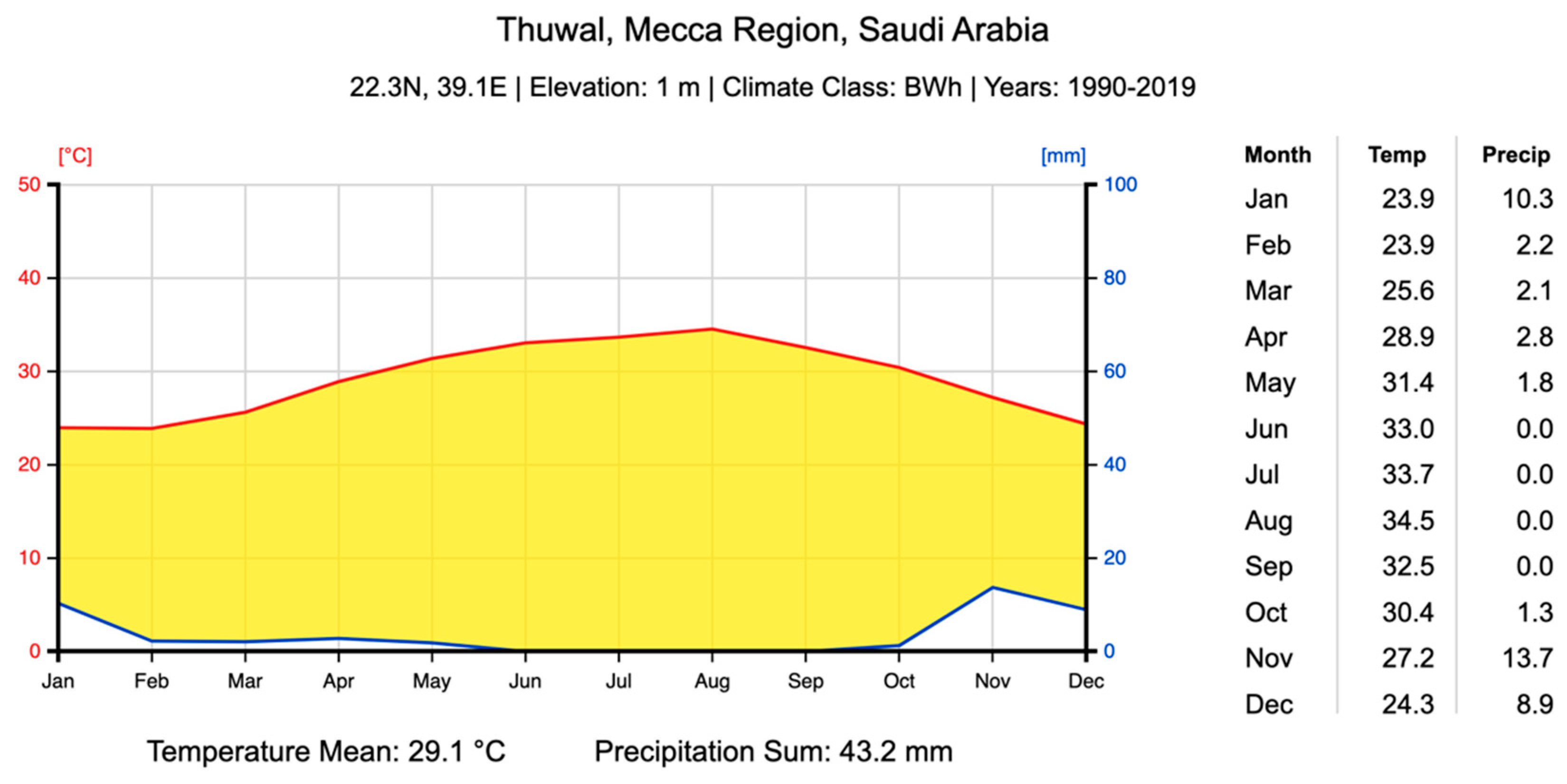
Figure 3.
K.A.CARE dataset correlation matrix for lagged features (last 3 hours).
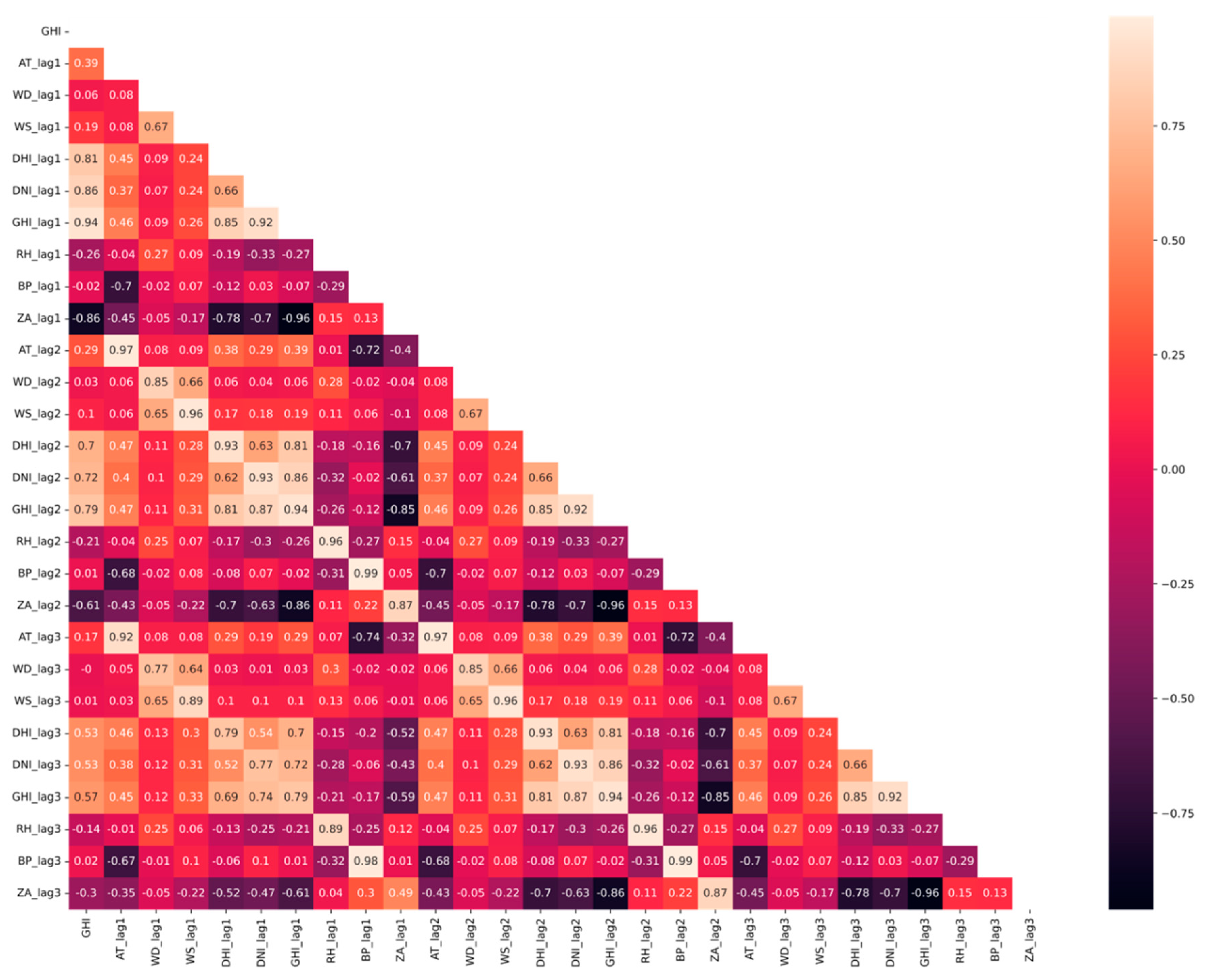
Figure 4.
K.A.CARE dataset correlation matrix for lagged features (last 1 day-360 days).
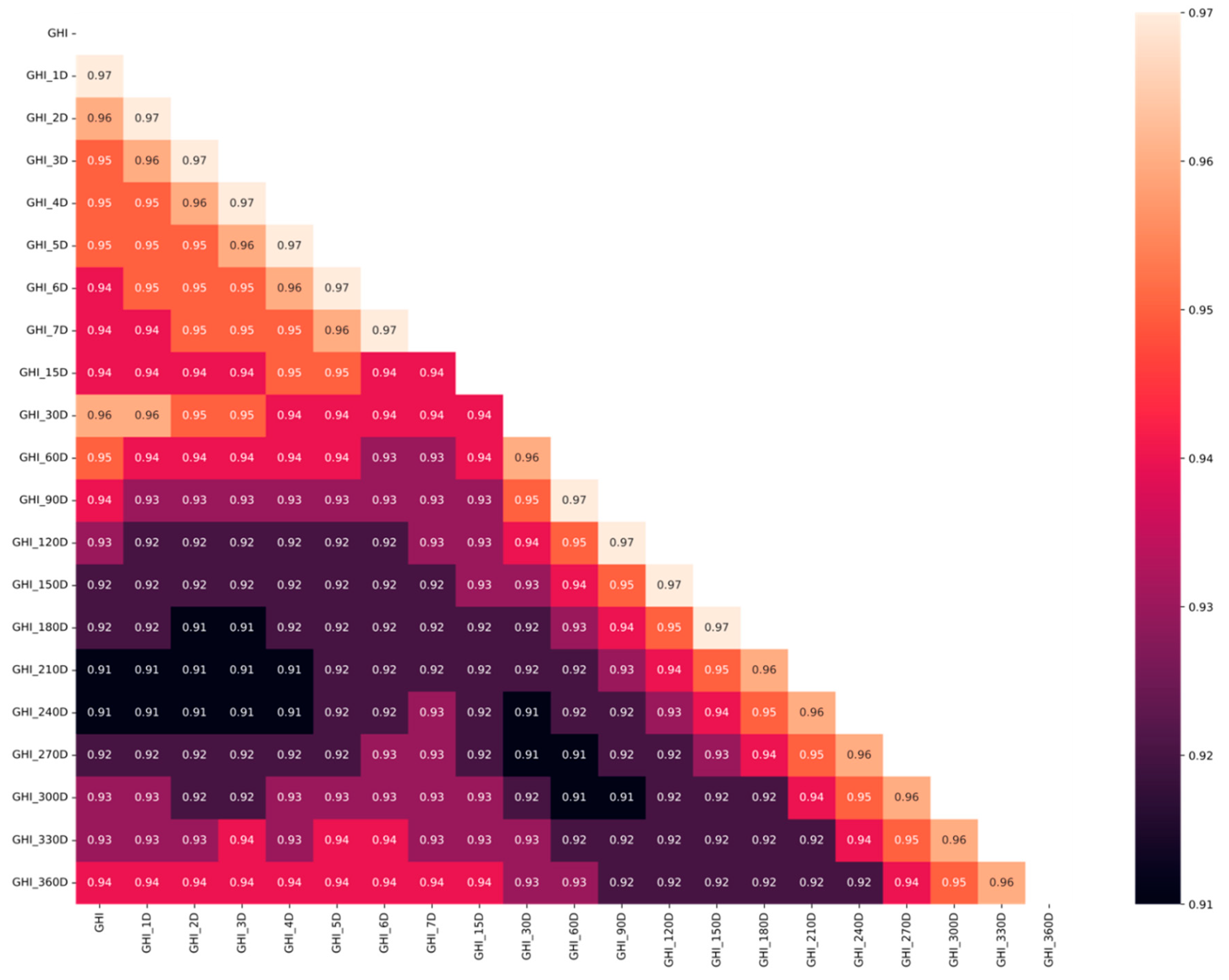
Figure 5.
AREONET and K.A.CARE merged dataset correlation matrix.
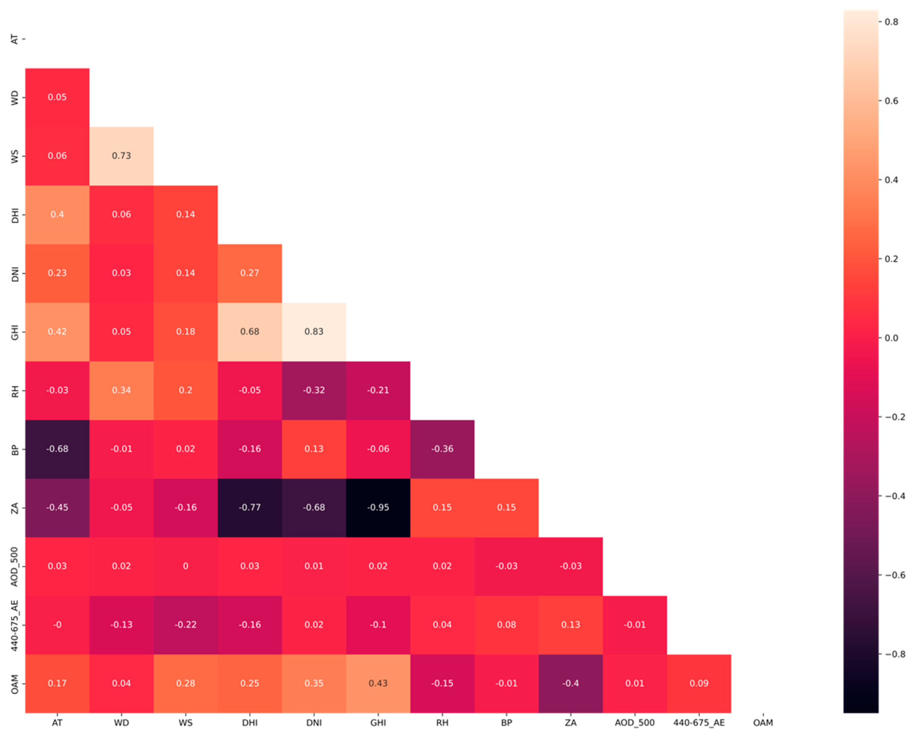
Figure 6.
(a) Clear day vs. (b) Dusty day (AREONET and K.A.CARE merged dataset).
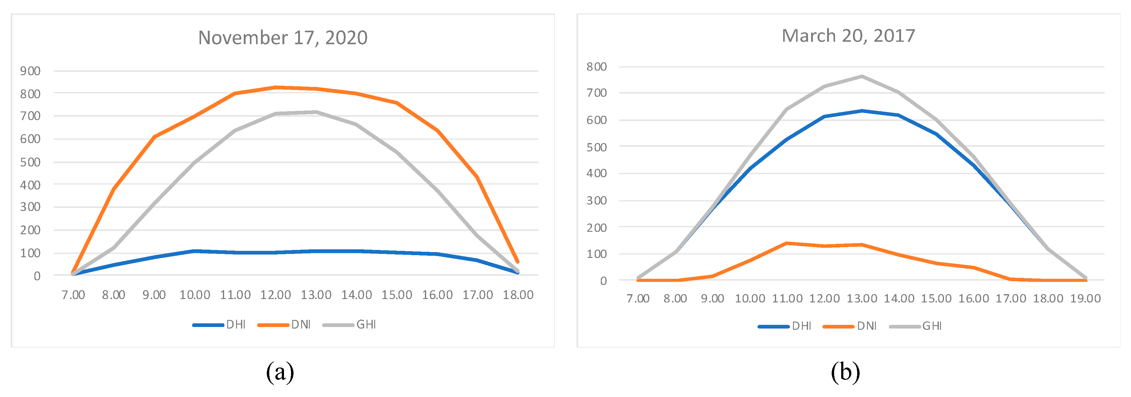
Figure 7.
NSRDB dataset correlation matrix for lagged features (last 3 hours).
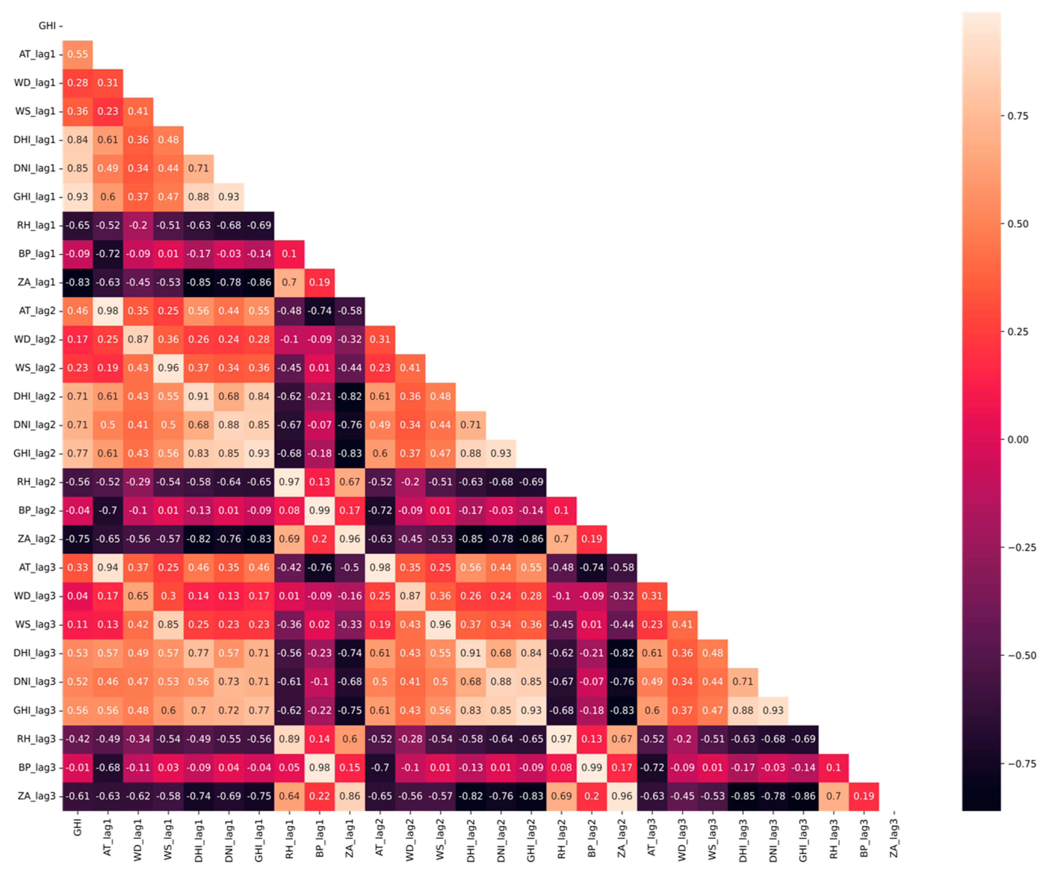
Figure 8.
NSRDB dataset correlation matrix for lagged features (last 1 day-360 days).
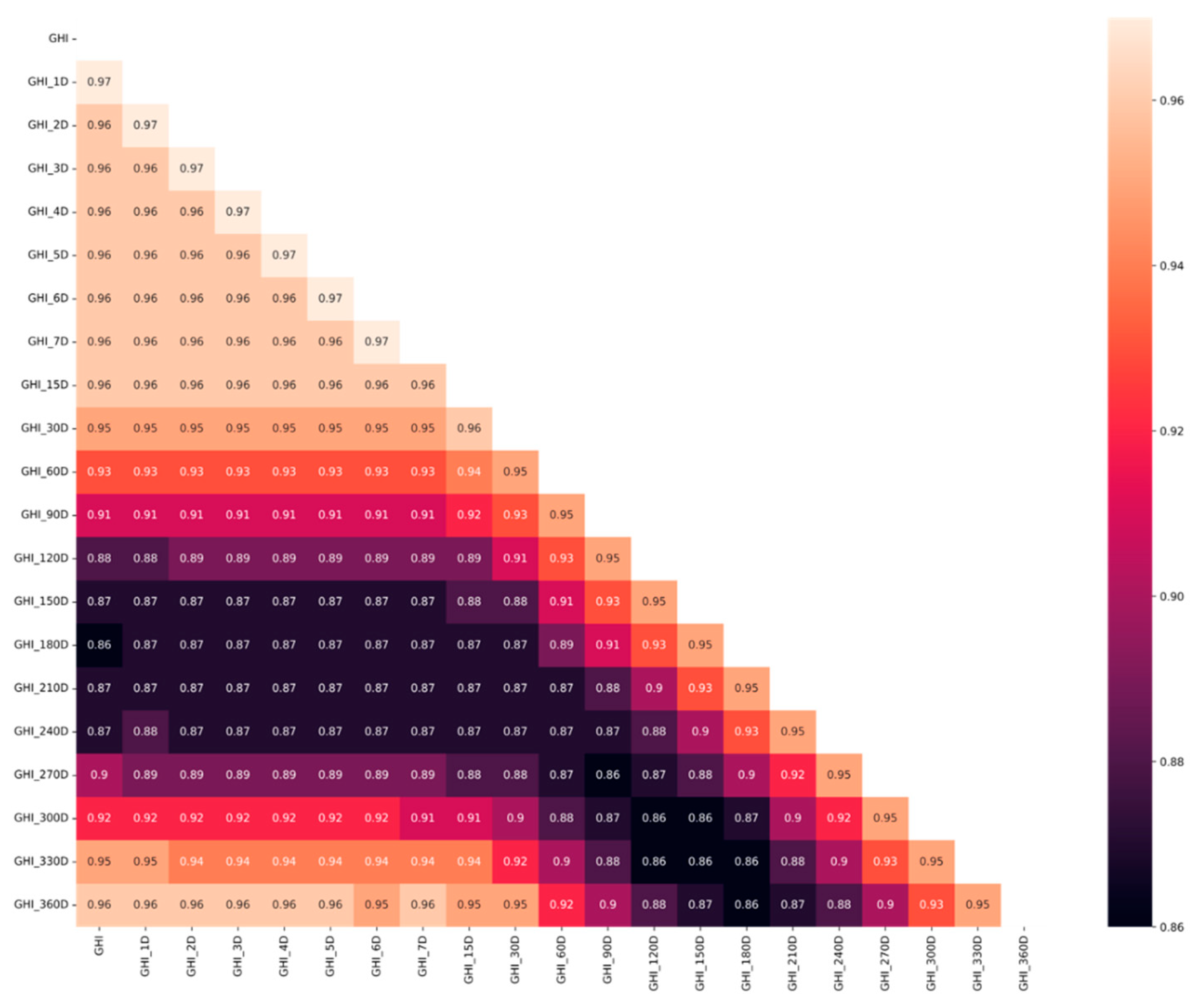
Figure 9.
NSRDB & GIOVANNI merged dataset correlation matrix.
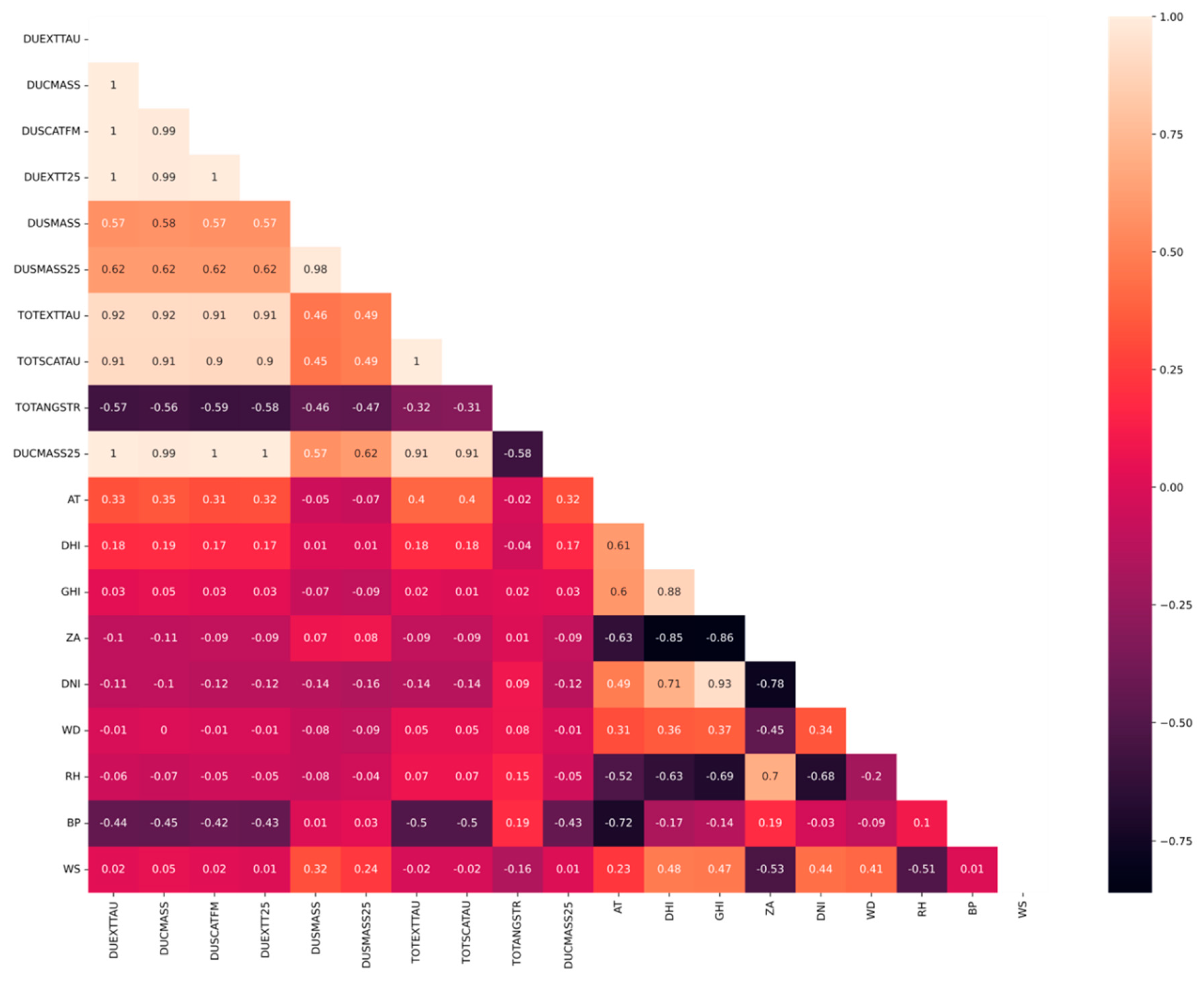
Figure 10.
(a) Clear day vs. (b) Dusty day (NSRDB & GIOVANNI merged dataset).
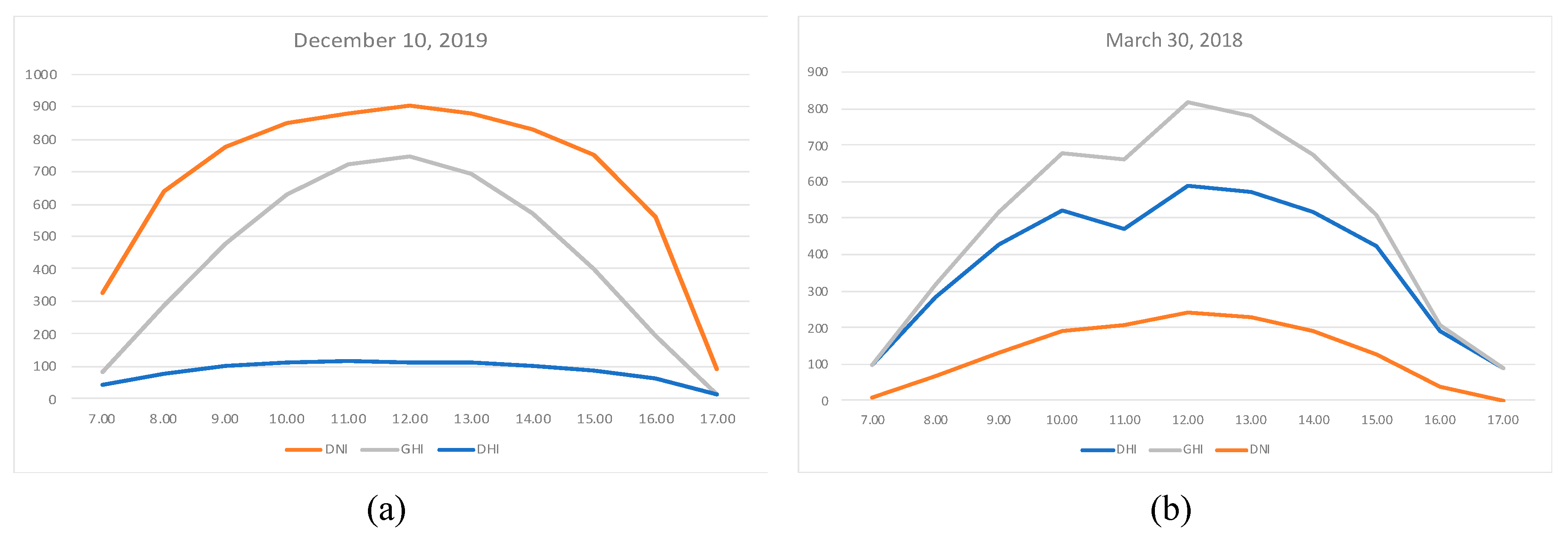
Figure 11.
LSTM model summary.
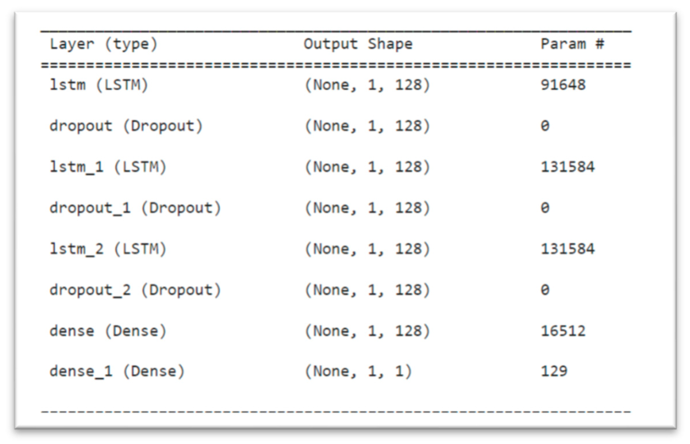
Figure 12.
GRU model summary.
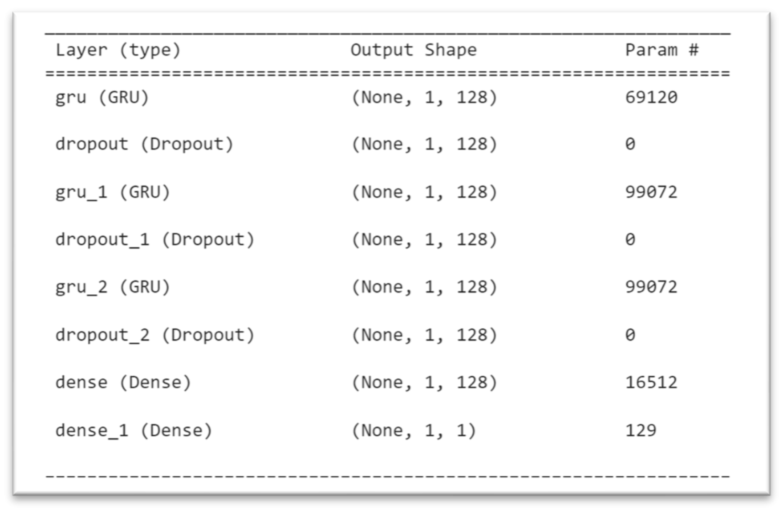
Figure 13.
BiLSTM model summary.
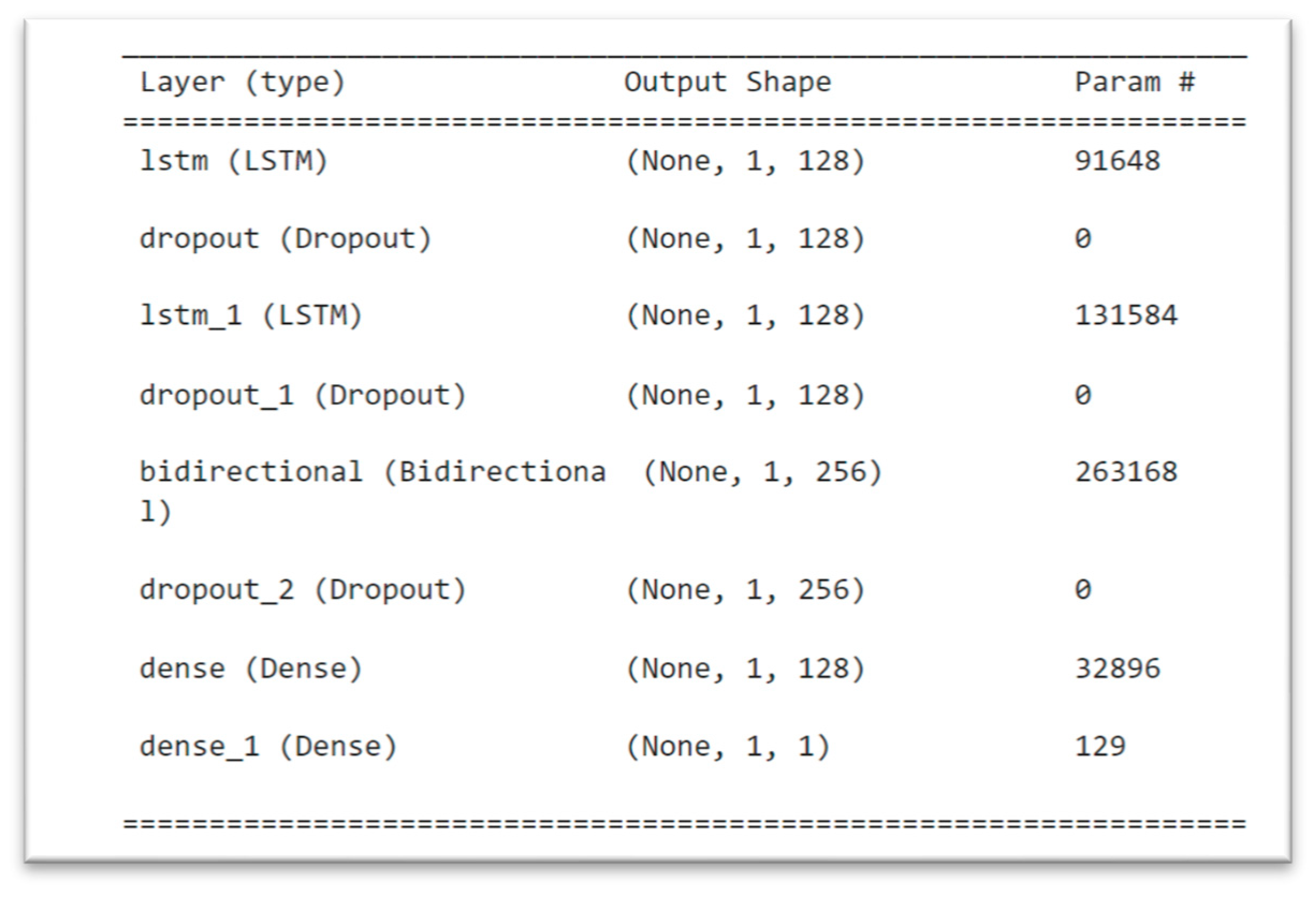
Figure 14.
BiGRU model summary.
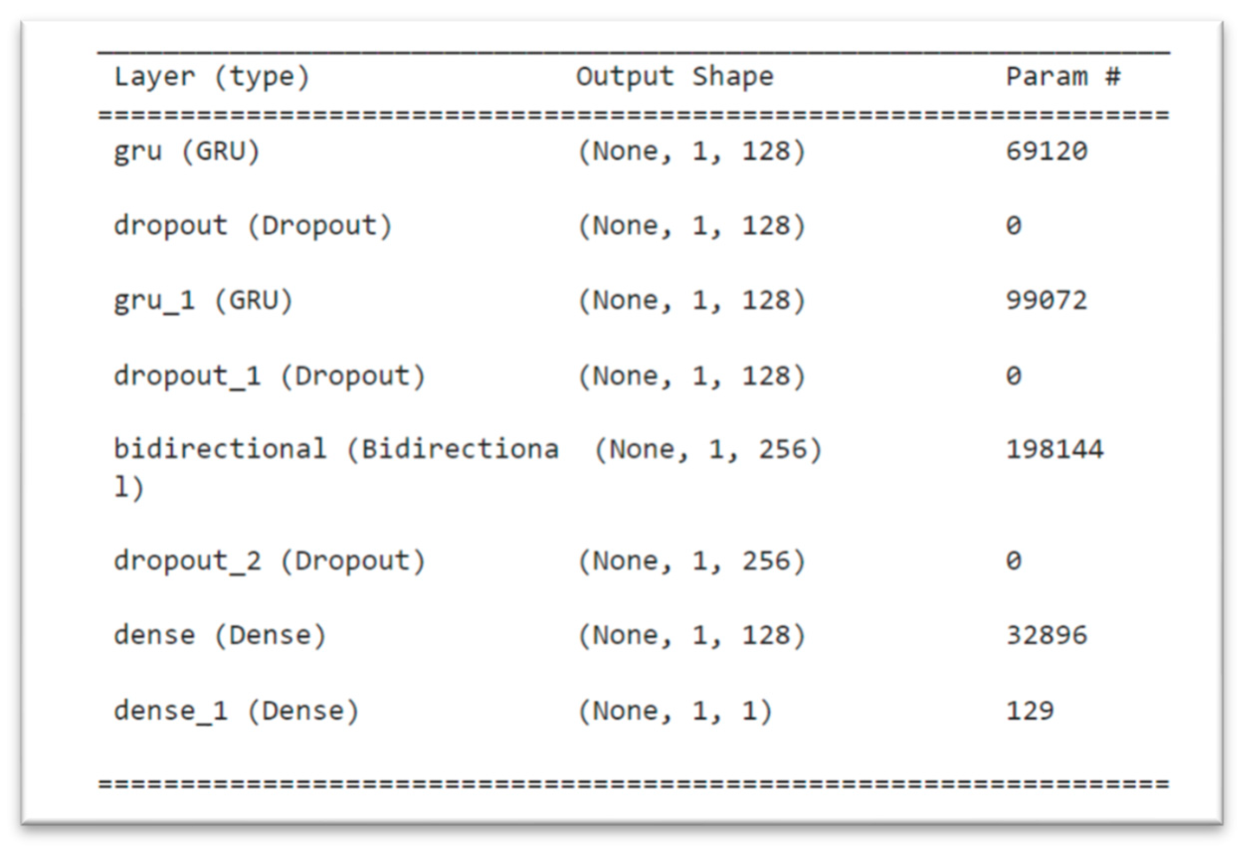
Figure 15.
LSTM-AE model summary.
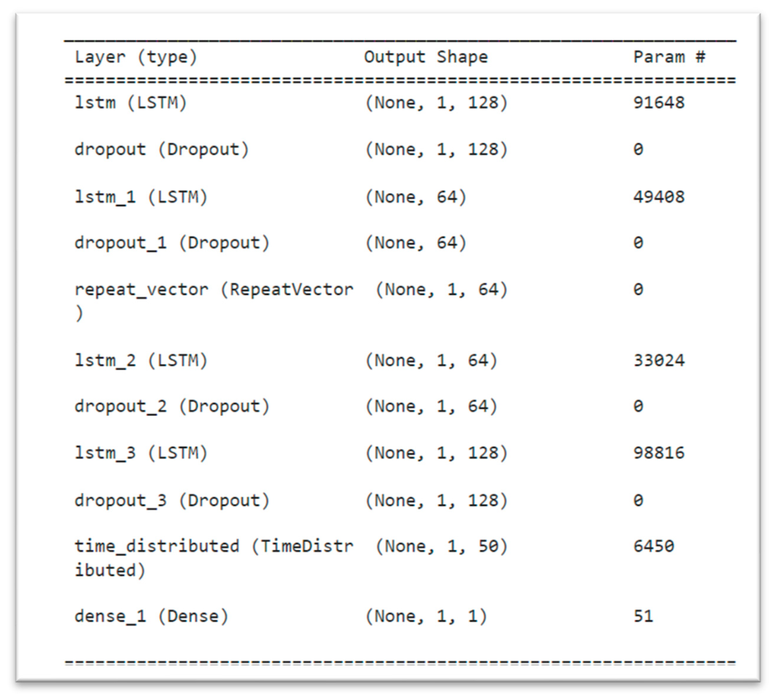
Figure 16.
Effect of lagged GHI (experiment 1, 2 & 3 RMSE results).
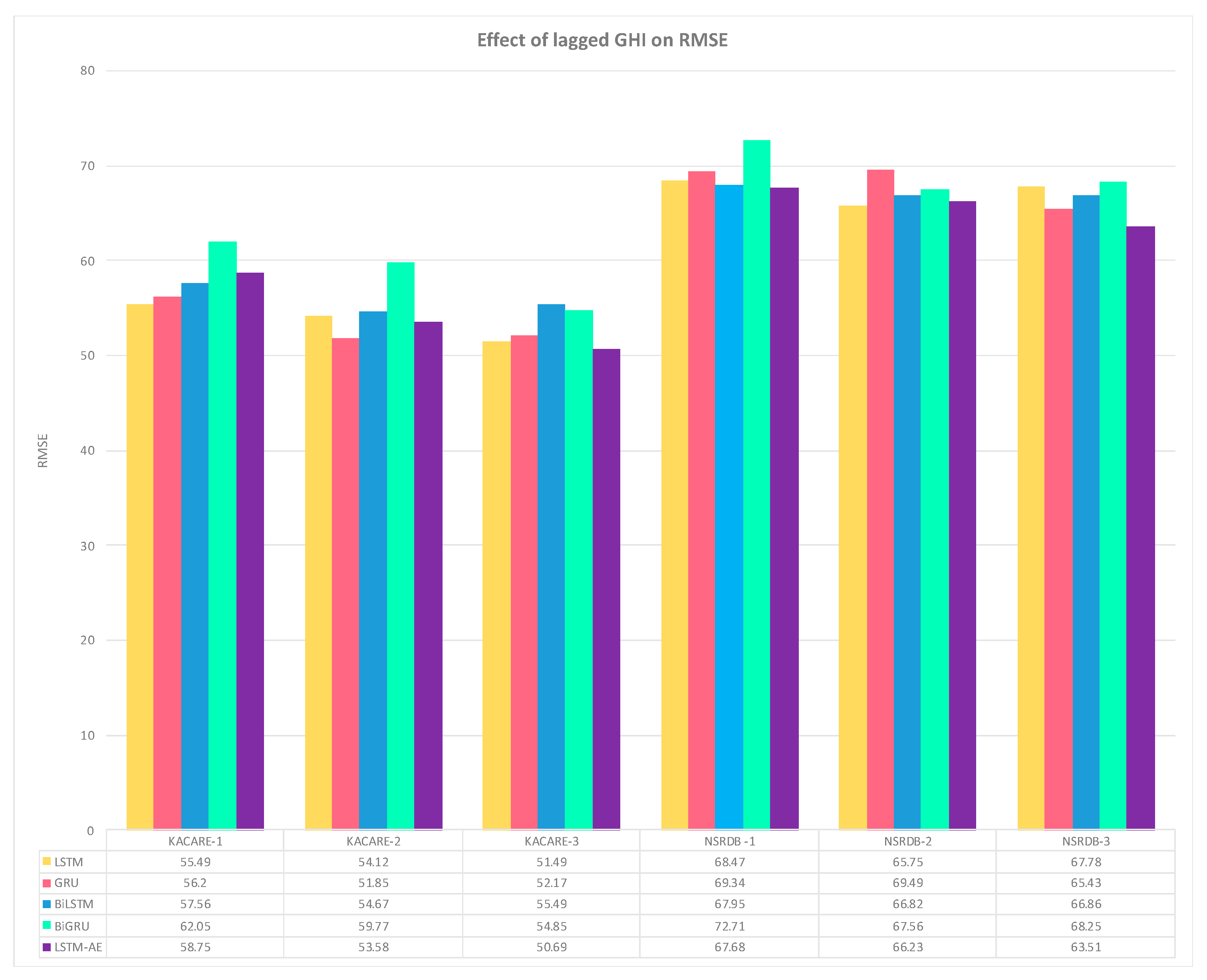
Figure 17.
Effect of lagged GHI (experiment 1, 2 & 3 MAE results).
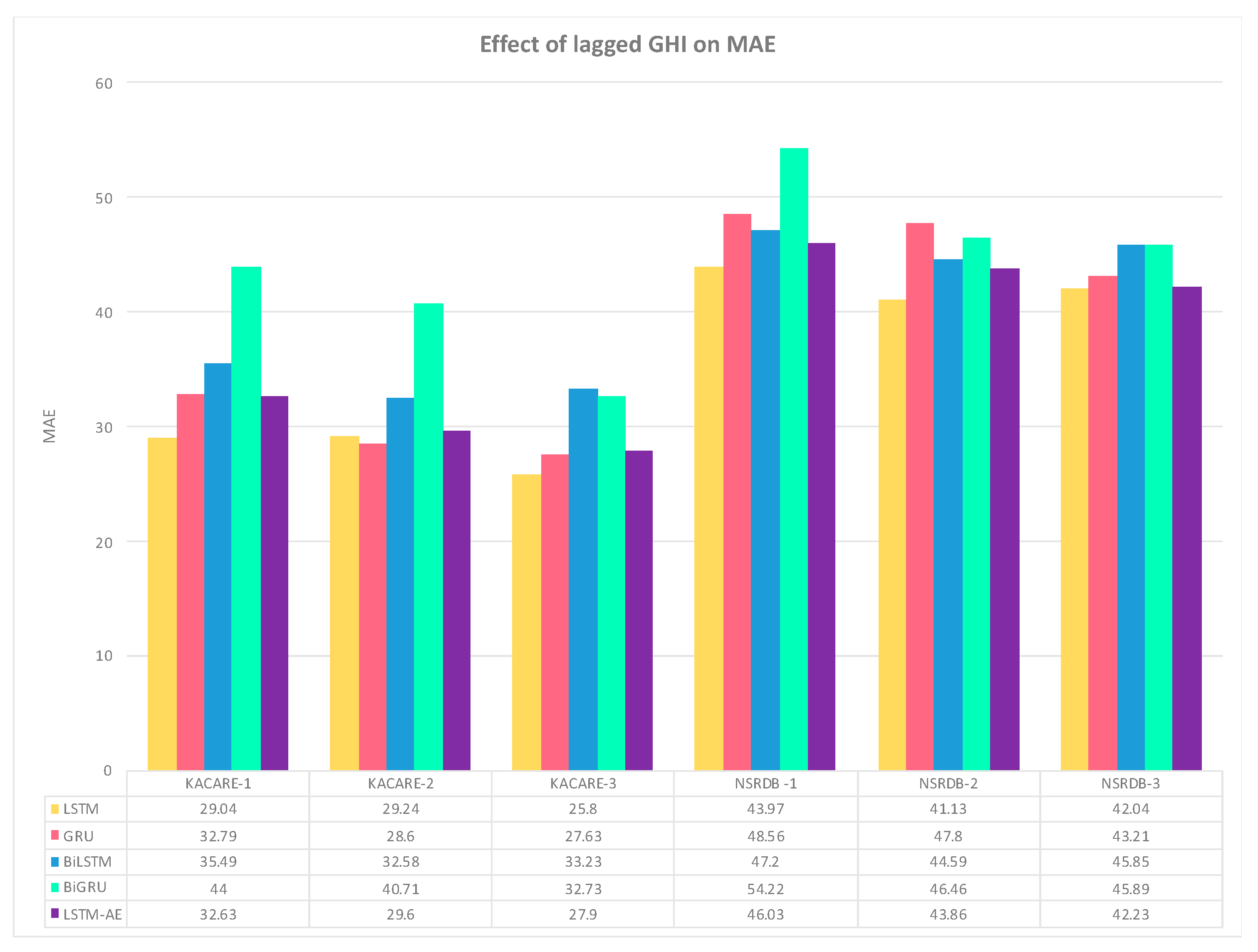
Figure 18.
Effect of lagged GHI (experiment 1, 2 & 3 MAPE results).
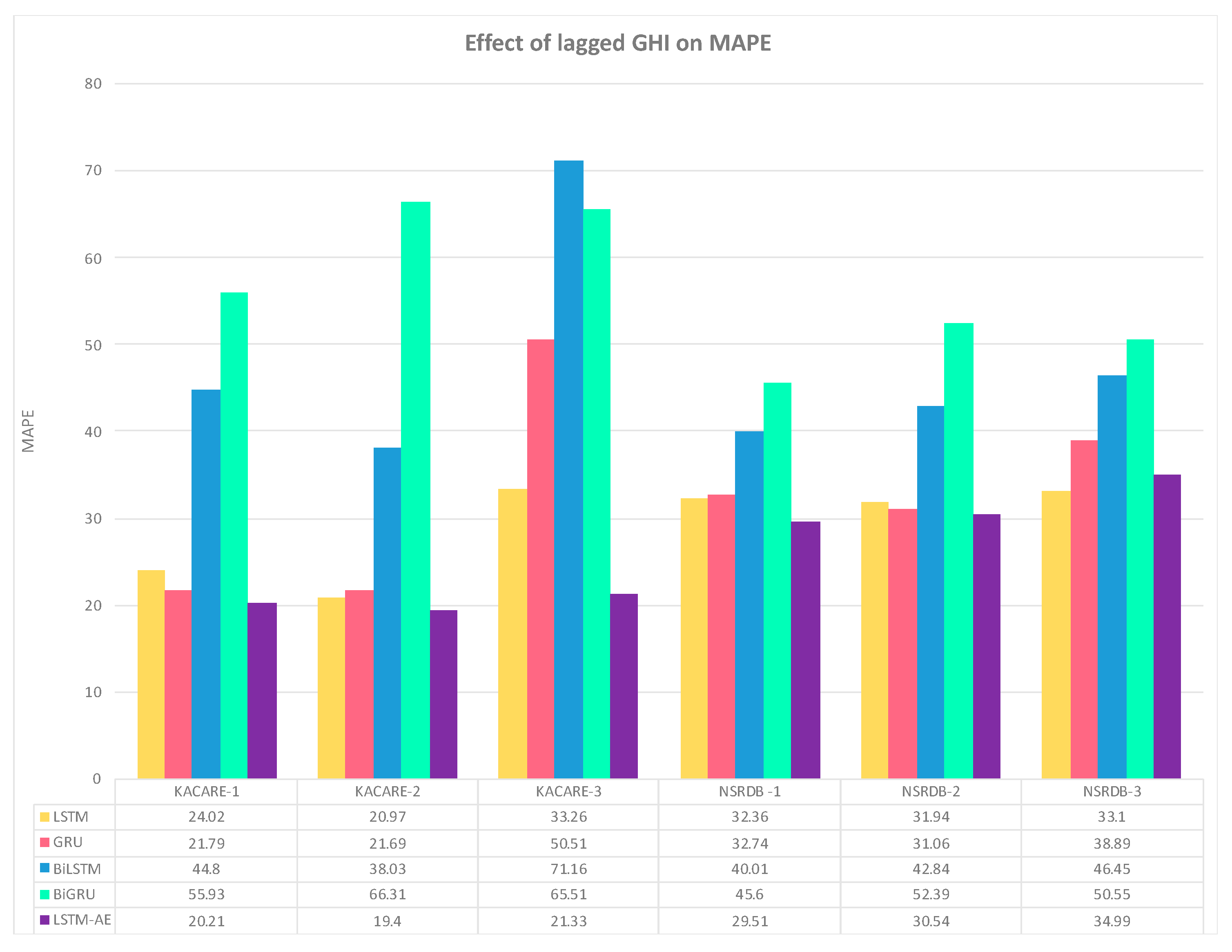
Figure 19.
Effect of weather (experiment 1 vs. experiment 2 RMSE results).
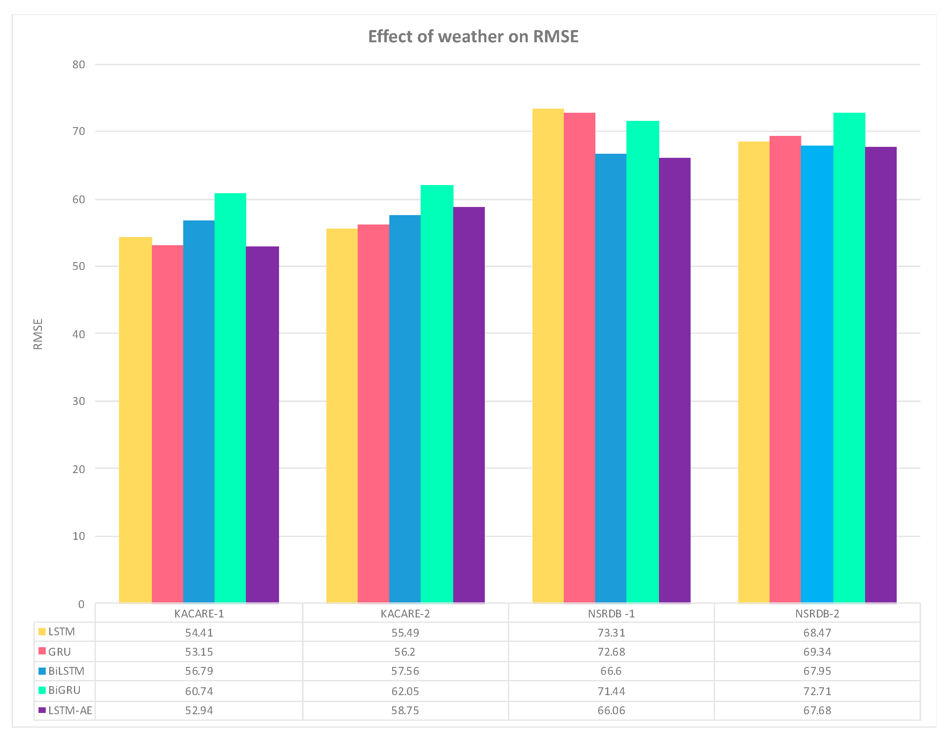
Figure 20.
Effect of weather (experiment 1 vs. experiment 2 MAE results).
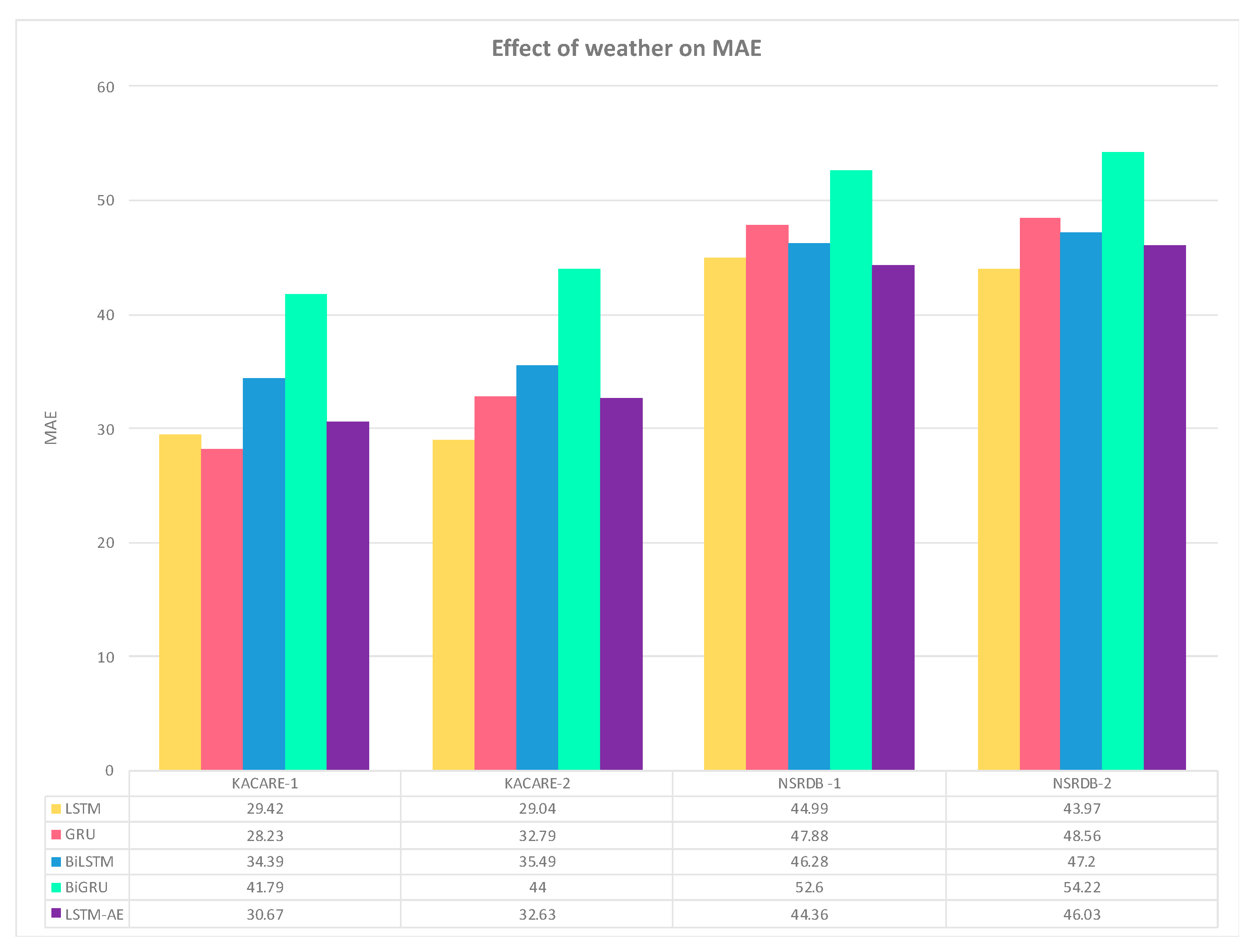
Figure 21.
Effect of weather (experiment 1 vs. experiment 2 MAPE results).
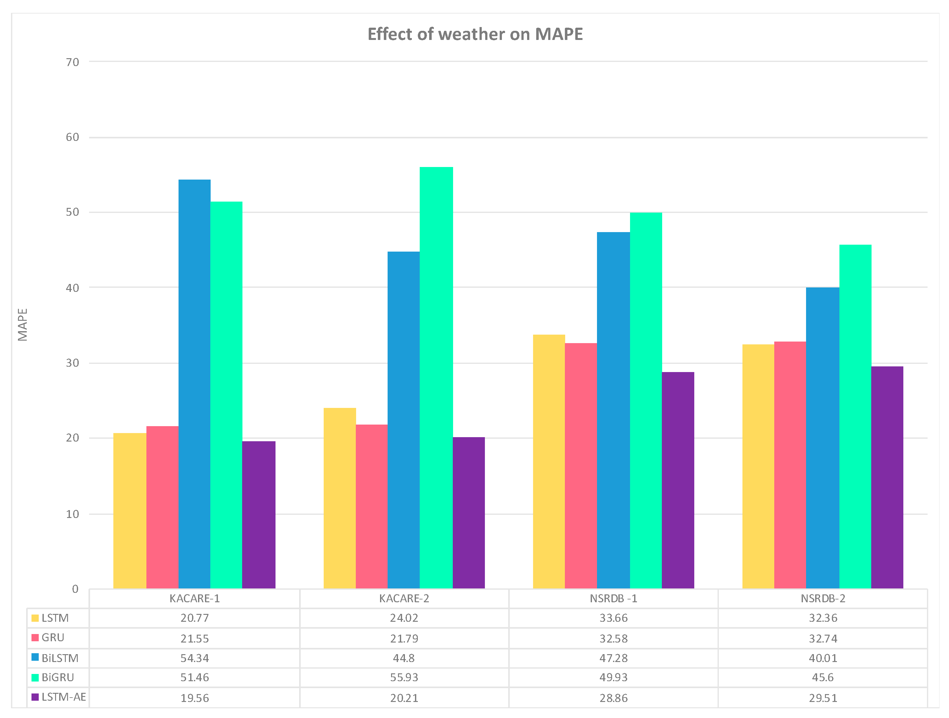
Figure 22.
Effect of aerosol (experiment 1 vs. experiment 2 RMSE results).
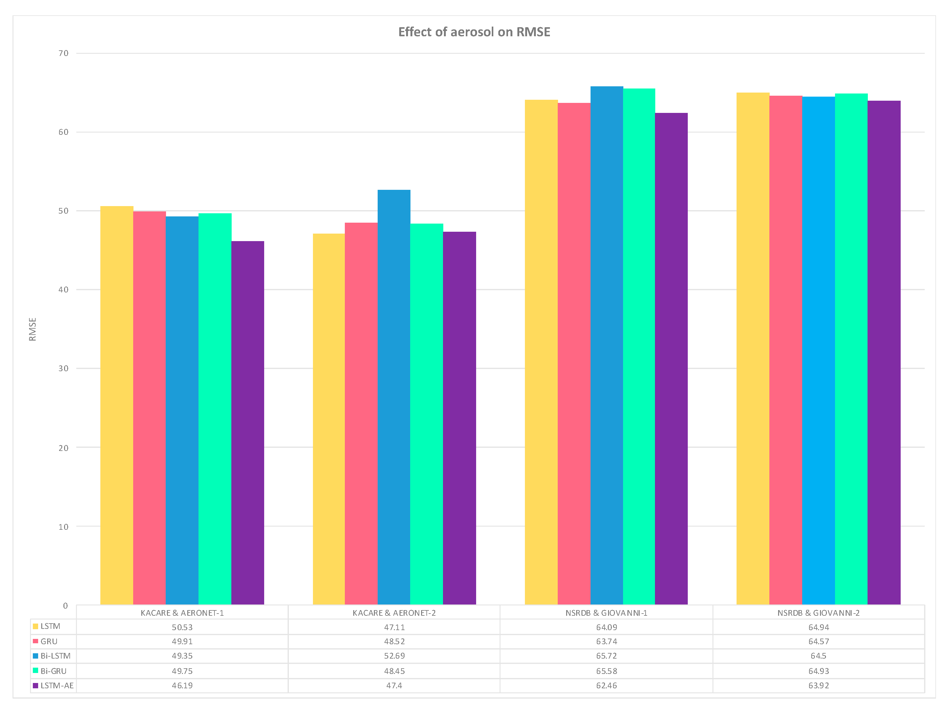
Figure 23.
Effect of aerosol (experiment 1 vs. experiment 2 MAE results).
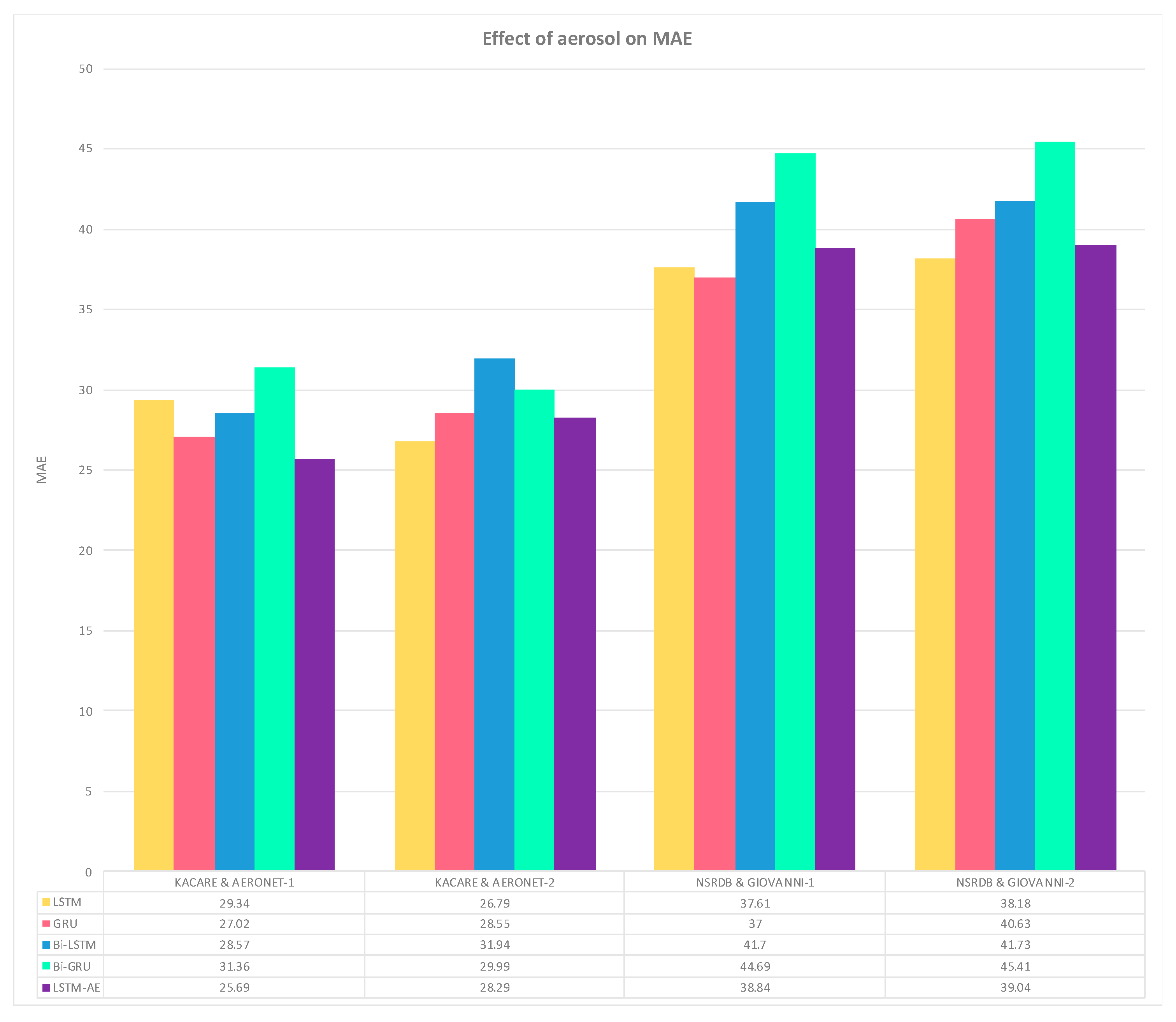
Figure 24.
Effect of aerosol (experiment 1 vs. experiment 2 MAPE results).
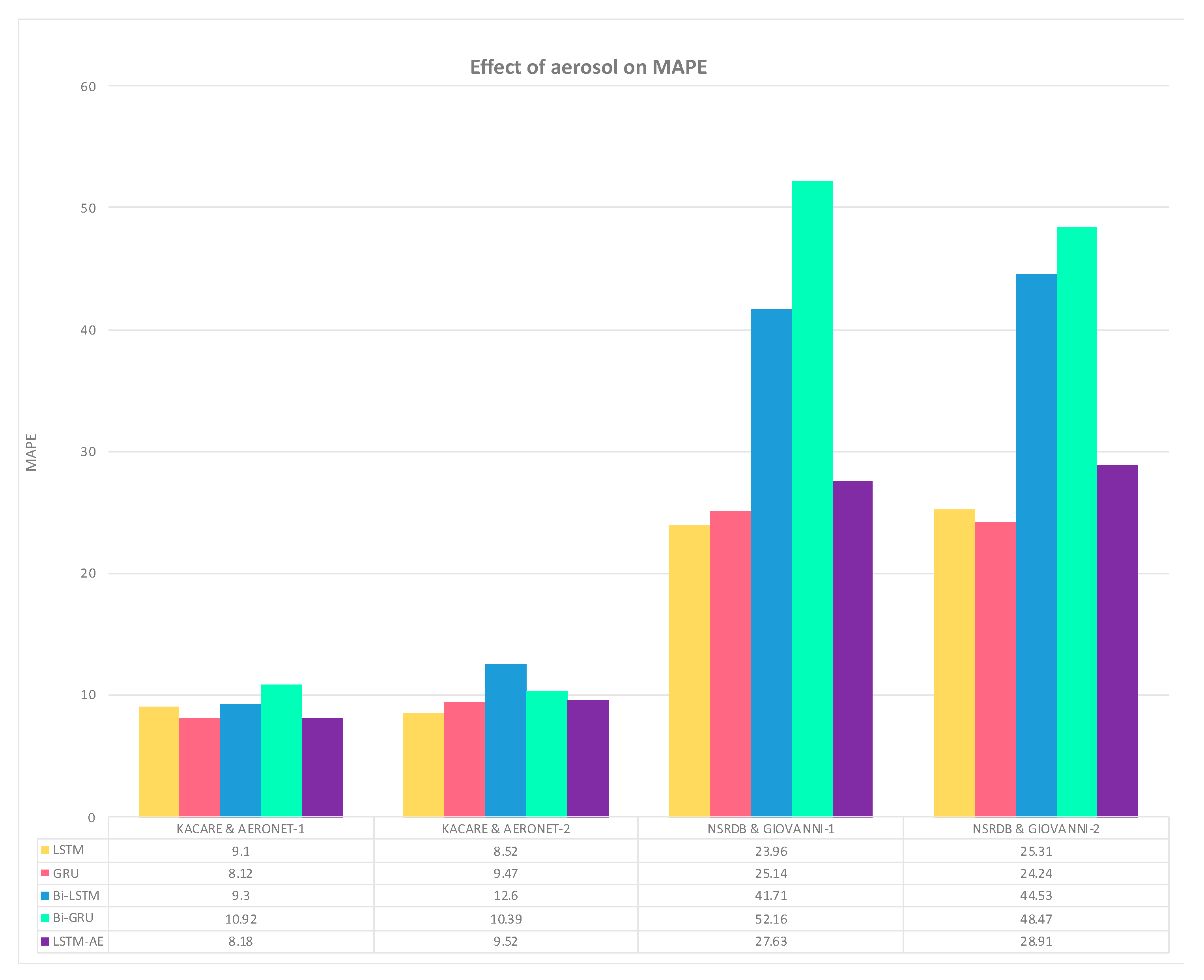
Figure 25.
FS of LSTM model (all experiments).
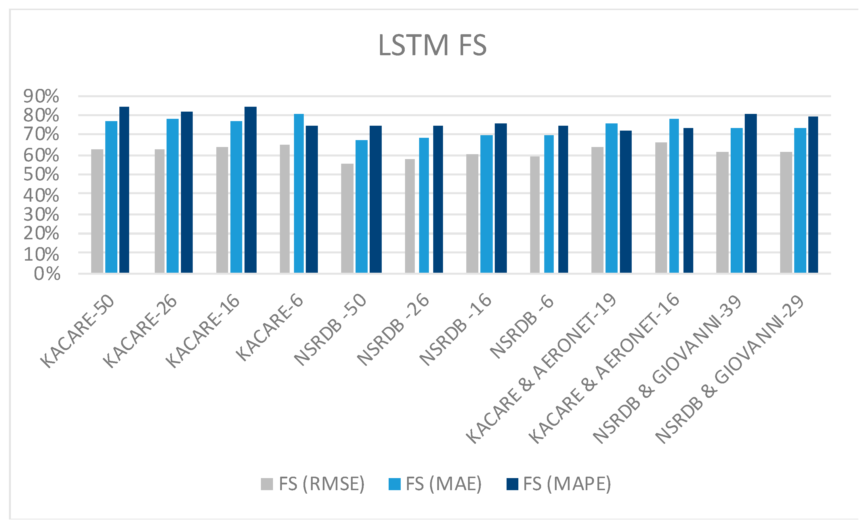
Figure 26.
Forecast skill of GRU model (all experiments).
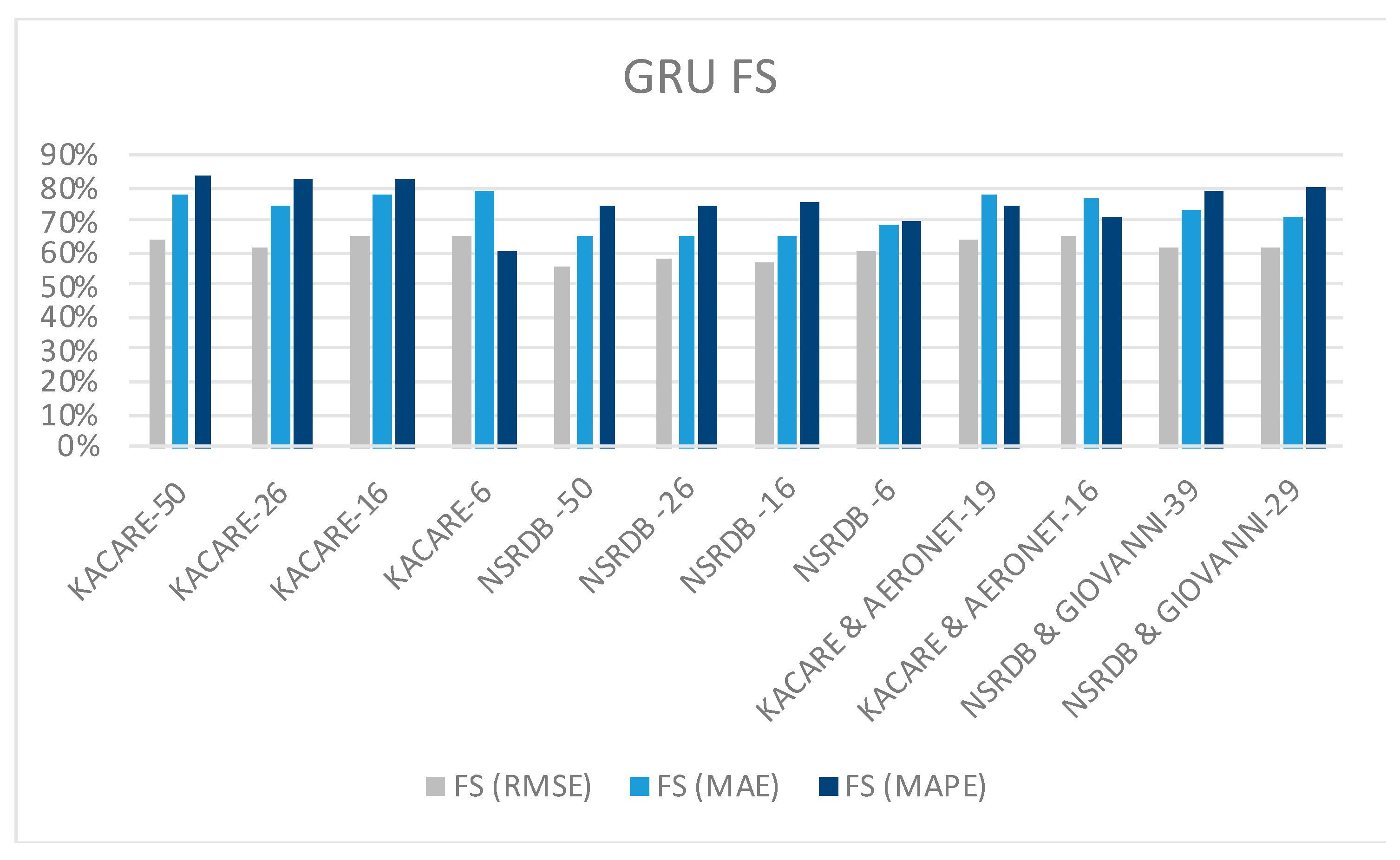
Figure 27.
Forecast skill of BiLSTM model (all experiments).
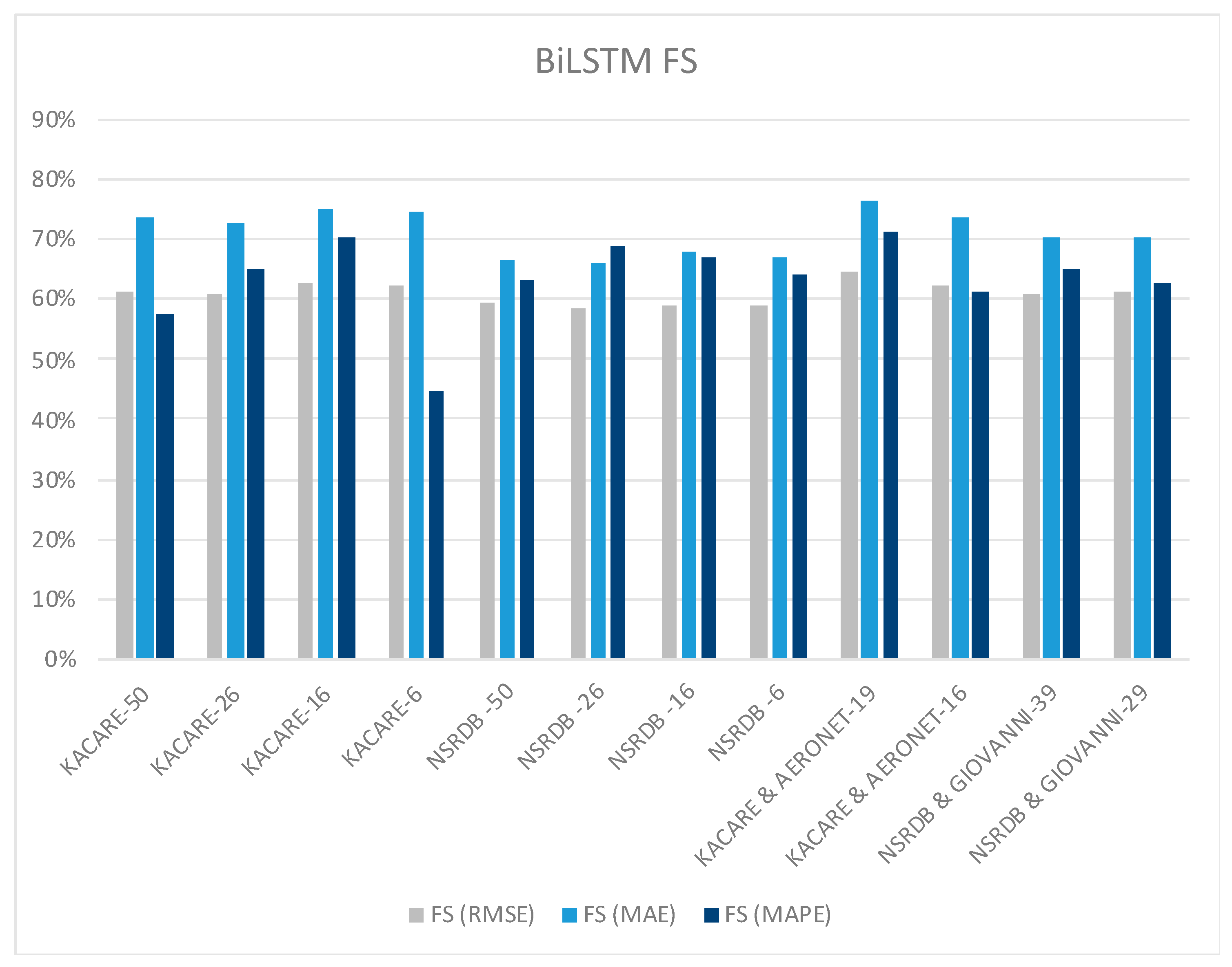
Figure 28.
Forecast skill of BiGRU model (all experiments).
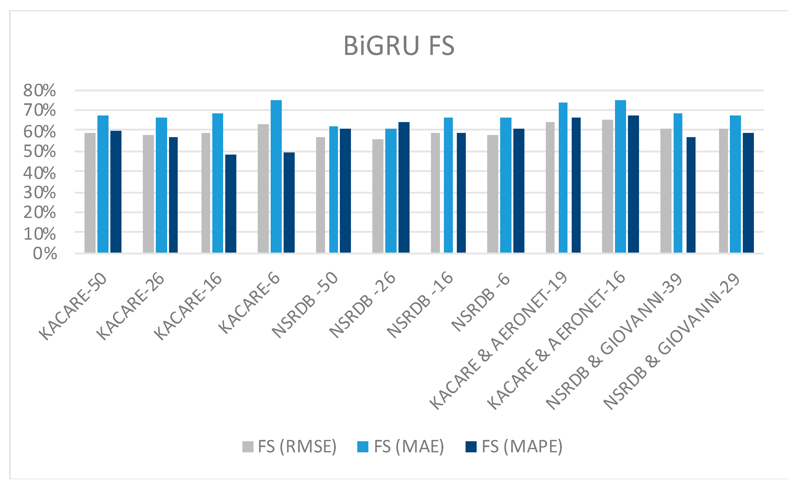
Figure 29.
Forecast skill of LSTM-AE model (all experiments).
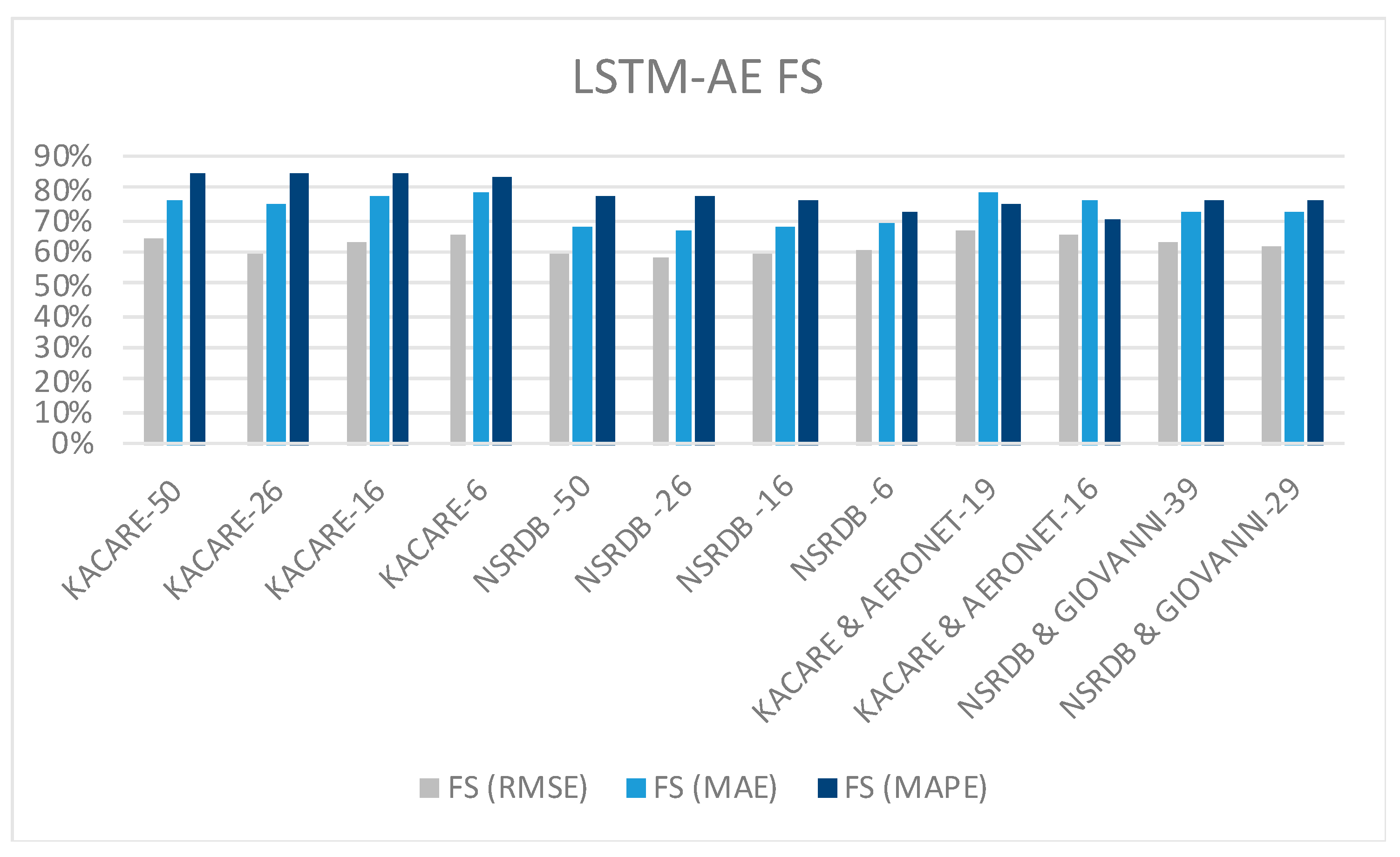
Table 1.
Related work summary.
| Ref No. | Method | Features | Data source | Results |
|---|---|---|---|---|
| [21] | Hybrid of CNN and LSTM, LSTM-AE | Date, time, location, inverter ID & temperature, power, slope irradiation, horizontal surface irradiation, ground temperature, AT, WS, RH | Ground-based | Hybrid CNN+LSTM model achieved the lowest MAPE= 13.42, RMSE=0.0987, and MAE=0.0506 for next-hour solar power prediction at South Korea. |
| [22] | CNN, LSTM | Hour, previous GHI; forecast of UV index, CC, DP, AT, RH, wind bearing, sunshine duration | Ground-based, satellite-based | Both CNN and LSTM models achieved the lowest normalized RMSE of around 43, and normalized MAE of around 17 for next-hour GHI prediction at Torino, Italy. |
| [23] | RBFNN, LSTM | Previous 30 days of AT, RH, P, ZA, GHI | Satellite-based | LSTM model without weather data achieved better RMSE= 0.013 for day ahead GHI prediction at Halifax, Canada and Tripoli, Libya |
| [24] | LSTM | Previous 24 hours of Clear sky GHI, DNI, DHI, RH | Satellite-based | LSTM model with four features achieved RMSE between 1.09% and 3.19% for day ahead GHI prediction at four locations in Canada |
| [31] | MLP, SVR, kNN, DTR | Last hour GHI, AOD, AE, DNI, DHI; current ZA, hour, month; forecast of WD, WS, AOD | Ground-based, satellite-based |
MLP model achieved the lowest RMSE= 32.75 and the highest FS= 42.10% for next-hour GHI prediction at Riyadh, Saudi Arabia. |
| [32] | ANN | AT, WS, WD, RH, P, AOD, GHI | Ground-based | ANN model achieved MSE=4.67% for next 3-hour GHI prediction at Delhi, India. |
| [33] | Autoregressive, SVR, LSTM | Last 10 min clear sky index; current clear sky index, CC, RH, AOD | Satellite-based | LSTM model achieved normalized RMSE=15.25% for next 10-min GHI prediction at a town in inner Mongolia. |
| [34] | Hybrid of CNN & MLP | Last 4 hours GHI; current AT, RH, ZA, AOD, WS, rainfall, P; sky images | Ground-based, satellite images | Hybrid CNN+MLP model achieved RMSE of around 38 and MAE of around 27 for next-hour GHI prediction at Shandong province, China |
| [35] | Ensemble of multiple regression, SVR, & MLP | ZA, AOD, P, AT, RH, WS, sine of day, CC, air mass, azimuth angle | Satellite-based | Ensemble model of multiple regression, SVR & MLP achieved normalized RMSE=21.98% and normalized MAE=11.13% for next 10-min GHI prediction at Golden City, USA. |
Table 2.
K.A.CARE dataset features.
| Time t features | Time t-1 features | Time t-2 features |
Time t-3 features |
Tim t features last n days | |
|---|---|---|---|---|---|
| GHI (output) |
GHI_lag1 | GHI_lag2 | GHI_lag3 | GHI_1D | GHI_90D |
| DNI_lag1 | DNI_lag2 | DNI_lag3 | GHI_2D | GHI_120D | |
| Hour | DHI_lag1 | DHI_lag2 | DHI_lag3 | GHI_3D | GHI_150D |
| Day | AT_lag1 | AT_lag2 | AT_lag3 | GHI_4D | GHI_180D |
| Month | ZA_lag1 | ZA_lag2 | ZA_lag3 | GHI_5D | GHI_210D |
| WS_lag1 | WS_lag2 | WS_lag3 | GHI_6D | GHI_240D | |
| WD_lag1 | WD_lag2 | WD_lag3 | GHI_7D | GHI_270D | |
| RH_lag1 | RH_lag2 | RH_lag3 | GHI_15D | GHI_300D | |
| BP_lag1 | BP_lag2 | BP_lag3 | GHI_30D | GHI_330D | |
| GHI_60D | GHI_360D | ||||
Table 4.
NSRDB & GIOVANNI dataset features.
| Time t features | Time t-1 features | Time t-2 & t-3 features |
Tim t features last n days | |
|---|---|---|---|---|
| GHI (output) | GHI_lag1 | DUEXTTAU_lag1 | GHI_lag2 | GHI_1D |
| DNI_lag1 | DUEXTT25_lag1 | DNI_lag2 | GHI_2D | |
| Hour | DHI_lag1 | TOTEXTTAU_lag1 | DHI_lag2 | GHI_3D |
| Day | AT_lag1 | DUCMASS_lag1 | ZA_lag2 | GHI_4D |
| Month | ZA_lag1 | DUCMASS25_lag1 | AT_lag2 | GHI_5D |
| WS_lag1 | DUSMASS_lag1 | GHI_lag3 | GHI_6D | |
| WD_lag1 | DUSMASS25_lag1 | DNI_lag3 | GHI_7D | |
| RH_lag1 | DUSCATFM_lag1 | DHI_lag3 | ||
| BP_lag1 | TOTSCATAU_lag1 | ZA_lag3 | ||
| TOTANGSTR_lag1 | AT_lag3 | |||
Table 5.
Datasets description.
| Dataset | Period | Missing days | Total Hourly Records | GHI mean | GHI SD | GHI var | Weather conditions |
|---|---|---|---|---|---|---|---|
| K.A.CARE | 24/12/2016- 03/03/2021 |
1117 days | Train: 7044 | 457.32 | 297.34 | 88411.98 | 1: 5458 2: 3090 3: 1499 |
| Val: 1495 | 424.40 | 269.23 | 72482.13 | ||||
| Test: 1508 | 446.66 | 293.61 | 86205.48 | ||||
| Total: 10047 | 450.82 | 292.97 | 85830.41 | ||||
| NSRDB | 27/12/2017- 31/12/2019 |
360 | Train: 6193 | 481.73 | 313.90 | 98534.76 | 1: 4548 2: 2780 3: 1504 |
| Val: 1314 | 529.09 | 331.09 | 109624.53 | ||||
| Test: 1325 | 438.84 | 278.12 | 77354.06 | ||||
| Total 8832 | 482.35 | 312.40 | 97595.1 | ||||
| K.A.CARE & AERONET | 05/01/2016- 03/03/2021 |
1215 days | Train: 2733 | 604.08 | 257.75 | 66436.59 | 1: 2508 2:1279 3:111 |
| Val: 580 | 607.67 | 260.03 | 67615.76 | ||||
| Test: 585 | 555.42 | 223.30 | 49863.17 | ||||
| Total: 3898 | 597.31 | 253.78 | 64405.57 | ||||
| NSRDB & GIOVANNI | 08/01/2017- 31/12/2019 |
7 days |
Train: 9180 | 473.20 | 309.68 | 95905.06 | 1: 6491 2: 4291 3: 2310 |
| Val: 1948 | 530.51 | 326.67 | 106714.98 | ||||
| Test: 1964 | 462.27 | 299.18 | 89503.37 | ||||
| Total: 13092 | 480.09 | 311.45 | 96998.23 | ||||
| *1=sunny, 2= partly clear, 3= unclear | |||||||
Table 6.
Effect of lagged GHI (experiment 1 vs. experiment 2 vs. experiment 3 features).
| Experiment 1 | Experiment 2 | Experiment 3 | |||
|---|---|---|---|---|---|
| GHI (output) | GHI_1D | GHI_90D | GHI (output) |
GHI_1D | GHI (output) |
| Hour | GHI_2D | GHI_120D | Hour | GHI_2D | Hour |
| Day | GHI_3D | GHI_150D | Day | GHI_3D | Day |
| Month | GHI_4D | GHI_180D | Month | GHI_4D | Month |
| GHI_lag1 | GHI_5D | GHI_210D | GHI_lag1 | GHI_5D | GHI_lag1 |
| GHI_lag2 | GHI_6D | GHI_240D | GHI_lag2 | GHI_6D | GHI_lag2 |
| GHI_lag3 | GHI_7D | GHI_270D | GHI_lag3 | GHI_7D | GHI_lag3 |
| GHI_15D | GHI_300D | GHI_15D | |||
| GHI_30D | GHI_330D | GHI_30D | |||
| GHI_60D | GHI_360D | GHI_60D | |||
| Total: 26 features | Total: 16 features | Total: 6 features | |||
Table 7.
Effect of weather (experiment 1 vs. experiment 2 features).
| Experiment 1 | Experiment 2 | |||||||
|---|---|---|---|---|---|---|---|---|
| GHI (output) | GHI_lag1 | GHI_lag2 | GHI_lag3 | GHI_1D | GHI_90D | GHI (output) |
GHI_3D | GHI_120D |
| DNI_lag1 | DNI_lag2 | DNI_lag3 | GHI_2D | GHI_120D | GHI_4D | GHI_150D | ||
| DHI_lag1 | DHI_lag2 | DHI_lag3 | GHI_3D | GHI_150D | Hour | GHI_5D | GHI_180D | |
| Hour | AT_lag1 | AT_lag2 | AT_lag3 | GHI_4D | GHI_180D | Day | GHI_6D | GHI_210D |
| Day | ZA_lag1 | ZA_lag2 | ZA_lag3 | GHI_5D | GHI_210D | Month | GHI_7D | GHI_240D |
| Month | WS_lag1 | WS_lag2 | WS_lag3 | GHI_6D | GHI_240D | GHI_lag1 | GHI_15D | GHI_270D |
| WD_lag1 | WD_lag2 | WD_lag3 | GHI_7D | GHI_270D | GHI_lag2 | GHI_30D | GHI_300D | |
| RH_lag1 | RH_lag2 | RH_lag3 | GHI_15D | GHI_300D | GHI_lag3 | GHI_60D | GHI_330D | |
| BP_lag1 | BP_lag2 | BP_lag3 | GHI_30D | GHI_330D | GHI_1D | GHI_90D | GHI_360D | |
| GHI_60D | GHI_360D | GHI_2D | ||||||
| Total: 50 features | Total: 26 features | |||||||
Table 8.
Effect of aerosol experiment 1 vs. experiment 2 features (K.A.CARE & AERONET dataset).
| Experiment 1 | Experiment 2 | ||
|---|---|---|---|
| GHI (output) | GHI_4D | GHI (output) | GHI_lag1 |
| Hour | GHI_lag1 | Hour | DNI_lag1 |
| Day | DNI_lag1 | Day | DHI_lag1 |
| Month | DHI_lag1 | Month | ZA_lag1 |
| AOD_500_lag1 | ZA_lag1 | GHI_1D | AT_lag1 |
| 440-675_AE_lag1 | AT_lag1 | GHI_2D | WS_lag1 |
| OAM_lag1 | WS_lag1 | GHI_3D | WD_lag1 |
| GHI_1D | WD_lag1 | GHI_4D | RH_lag1 |
| GHI_2D | RH_lag1 | BP_lag1 | |
| GHI_3D | BP_lag1 | ||
| Total: 19 features | Total: 16 features | ||
Table 9.
Effect of aerosol experiment 1 vs. experiment 2 features (NSRDB & GIOVANNI dataset).
| Experiment 1 | Experiment 2 | |||||||
|---|---|---|---|---|---|---|---|---|
| GHI (output) | GHI_lag1 | DUEXTTAU_lag1 | GHI_lag2 | GHI_1D | GHI (output) | GHI_lag1 | GHI_lag2 | GHI_1D |
| DNI_lag1 | DUEXTT25_lag1 | DNI_lag2 | GHI_2D | DNI_lag1 | DNI_lag2 | GHI_2D | ||
| Hour | DHI_lag1 | TOTEXTTAU_lag1 | DHI_lag2 | GHI_3D | Hour | DHI_lag1 | DHI_lag2 | GHI_3D |
| Day | AT_lag1 | DUCMASS_lag1 | ZA_lag2 | GHI_4D | Day | AT_lag1 | ZA_lag2 | GHI_4D |
| Month | ZA_lag1 | DUCMASS25_lag1 | AT_lag2 | GHI_5D | Month | ZA_lag1 | AT_lag2 | GHI_5D |
| WS_lag1 | DUSMASS_lag1 | GHI_lag3 | GHI_6D | WS_lag1 | GHI_lag3 | GHI_6D | ||
| WD_lag1 | DUSMASS25_lag1 | DNI_lag3 | GHI_7D | WD_lag1 | DNI_lag3 | GHI_7D | ||
| RH_lag1 | DUSCATFM_lag1 | DHI_lag3 | RH_lag1 | DHI_lag3 | ||||
| BP_lag1 | TOTSCATAU_lag1 | ZA_lag3 | BP_lag1 | ZA_lag3 | ||||
| TOTANGSTR_lag1 | AT_lag3 | AT_lag3 | ||||||
| Total: 39 features | Total: 29 features | |||||||
Disclaimer/Publisher’s Note: The statements, opinions and data contained in all publications are solely those of the individual author(s) and contributor(s) and not of MDPI and/or the editor(s). MDPI and/or the editor(s) disclaim responsibility for any injury to people or property resulting from any ideas, methods, instructions or products referred to in the content. |
© 2024 by the authors. Licensee MDPI, Basel, Switzerland. This article is an open access article distributed under the terms and conditions of the Creative Commons Attribution (CC BY) license (http://creativecommons.org/licenses/by/4.0/).
Copyright: This open access article is published under a Creative Commons CC BY 4.0 license, which permit the free download, distribution, and reuse, provided that the author and preprint are cited in any reuse.


