Submitted:
09 January 2024
Posted:
10 January 2024
You are already at the latest version
Abstract
Multiple imputation with chained equations (MICE) is a widespread approach to account for missing data in empirical research. Combining MICE with bootstrapping, that is, repeatedly resampling with replacement from the data to estimate variances and confidence intervals of statistics of interest, is not straightforward. The current document provides an overview of how to use bootstrapping with imputed data in Stata. Two main approaches (impute first and then bootstrap or vice-versa) are discussed and shortly compared. Code is provided for Stata.
Keywords:
bootstrapping
; multiple imputation
; MICE
; stata
; missing data
Introduction
Bootstrapping imputed datasets
Missing data is a highly prevalent problem in applied statistics. Especially in the social sciences, where survey compliance is usually rather low nowadays, many people refuse participation completely or do not answer all questions, leaving researchers with gaps in their data. As soon as this missingness is correlated with an individual’s characteristics, bias is created which can lead to wrong conclusions. Imputing missing data before analyses is therefore required. One of the most prominent and well-researched approaches to this problem is multiple imputation with chained equations (MICE) as it is flexible and implemented in all common statistical software packages [1,2]. However, if one wants to combine imputed data with bootstrapping some complications arise. When using MICE, multiple datasets are created with random noise added in each. Bootstrapping is a process of resampling, usually from a single dataset [3,4]. As soon as multiple ones must be utilized, this basic approach has to be adapted. In the following, it is demonstrated how this can be achieved in Stata [5]. As there are two main approaches, both are outlined. While one has a clear advantage of computing time, the other might provide more valid results.
Complete data analysis
We start with the analysis of the complete dataset, that is, in the absence of any missingness. This is required to have a benchmark for the following analyses. By creating artificial missingness we have full control over the process and can arrive at valid conclusions and fair comparisons. The original dataset contains 500 individuals and seven variables, which are: hours worked per week (hours), time worked in the current job (tenure), total work experience (ttl_exp), educational achievement (grade) and current age (age). Furthermore, we have two variables about income: current income (wage) and income one year ago (wage0).
While bootstrapping can theoretically applied to virtually any analysis or statistic, we go for a regression model and want to bootstrap R-squared (R²). To be concrete, we will regress current wages on all other variables in the dataset (except for wage0, which is an auxiliary variable in the imputation model). Summarized, we try to explain whether the other variables are able to explain current wages. If the R-squared is large, this is the case. To compute the point estimate and the 95% confidence interval, we use the following code:
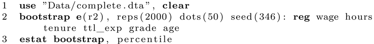
First, we open the dataset and run the bootstrap command. We inform Stata that we are interested in bootstrapping the R-squared statistic, which is saved in the regression command in e(r2). After the comma, the options for the bootstrap procedure are specified. Reps is the number of bootstrap resamples and a larger number will give more precise results. For most analyses, 500 replications should be the minimum but for precise results, more than 10,000 replications are advised if computational feasible [6]. Dots prints a dot every 50 replications so we can keep track of the process. A random seed ensures that the results are reproducible. Finally, after the colon, we list the command that is used to produce the statistic of interest. In this case it is an OLS regression model using regress or reg. After completion, Stata prints the results. The point estimate is listed under observed coefficient (Figure 1). Note that the printed confidence interval is based on the depicted standard error, which is usually not exactly what we want. By adding estat, we can generate more output and a percentile confidence interval. Stata reports CIs based on standard errors, percentiles or the BC/BCa method. In this example, we will stick with percentile. Interestingly, the bias is rather large, despite using a large number of replications. As a rule of thumb, the bias should be at most 25% of the bootstrap standard error. The main result is the CI, which is 11.40 to 23.91. The results using the imputed datasets should approximate this finding.
Amputing the data
Next, we create artificial missingess in the data to test how well our methods can account for this problem. As this is a demonstration, we have full control over the process and can compare our results to the original findings where no missingness is present. This is a huge advantage for simulations yet almost never the case in the real world. If your data contains missing values, it is usually not possible to state exactly why these values are missing. Yet, it is crucial that the missingness is either completely at random (MCAR) or missing at random (MAR). Only then, imputation attempts will lead to sensible and unbiased results. MCAR is usually a very strong assumption (a best case scenario, so to say) and can happen in surveys if questions are applied randomly. For example, to keep expenses down, researchers might flip a coin before interviewing and only 50% of all participants receive the complete questionnaire while the other half receives a reduced one which is faster to answer. This process guarantees that the respondent characteristics (and responses) and the missingness are completely due to randomness and hence, no bias is create (the statistical power of the analyses is nevertheless reduced). MAR means that the missingness can somehow be explained by other information in the data. For example, if individuals with a below-average wage have a higher propensity to refuse answering when asked about their income, this information is not missing at random. However, if one can plausible deduce the wage out of other respondent characteristics (such as the occupation or educational qualification of the individual), one can impute the missingness and amend the bias. This means, the source of missingness must somehow be correlated with other information in the data or model. As long as MAR holds, imputation methods can improve data quality.
In the following we will build a dataset where some variables are missing at random, that means, their missingness depends on the other variables in the data. We specify that age, ttl_exp hours, wage have missing data. The data are amputed using a logistic link function. Afterwards, the average missingness in the specified variables is 27%. However, if one would apply listwise deletion, one would end up with an effective sample size of only 180 observations since even having a single variable with a missing is enough to exclude this observation from the analysis, reducing the sample size massively. This is unacceptable.
Bootstrapping with imputed data
We will introduce two main approaches which enable us to apply bootstrapping to imputed data, which are BootImpute (BI) and ImputeBoot (IB). The first approach takes a random bootstrap sample from the data and then runs the imputation procedure, estimates the statistic of interest and stores the result. These steps are repeated many times to arrive at a bootstrap distribution. The second one imputes the data first and only a single time and then samples repeatedly from this imputed dataset. Both approaches are valid but work rather differently [7]. Before explaining each method some words are required about how the data must be imputed for this application in Stata.
Imputed data format
Note that the following examples are used with cross-sectional data and the data format is hence wide in Stata, where one individual / observation takes exactly one data row in the browser. When imputing data with Stata, one has, in theory, four different options to store the imputed data, which are different from the original (since the dataset then must contain the original information with missingness present and the imputed data where missing values are replaced). For the approaches shown it is crucial that the data are set to flong. What this means is that for each added imputation (M), a full dataset is stored. While this takes more space than other formats such as mlong, it makes the processing much more convenient. To better understand the data format, consider this toy dataset. Here, only two individuals are included with three variables (a, b, c). Individual 1 has valid information on all three variables, individual 2 has missings on b and c. After imputation in flong and generating two imputations (M=2), the dataset looks as follows:
Of greatest relevance is the system variable _mi_m, created by Stata. This variable tracks the imputation. 0 stands for the original datarows, which are untouched. The value 1 is for imputation 1 and so on. We see that each imputation contains also the observation which was not imputed since it had no missing values. While this format takes more space, it makes working with the data easy since we can simply loop over all imputed datasets, running from 1 to M, and compute the statistic of interest. Afterwards, these statistics are combined to arrive at a final imputed statistic.
Boot + Impute
We start with the BootImpute (BI) approach, which is conceptually easier to explain. One can summarize the algorithm as follows:
- Take a single random bootstrap resample from the original data. Naturally, this bootstrap sample will contain missing values when the original has also missing values.
- Run the imputation model on this bootstrap sample to fill in the missing values.
- Estimate the statistic of interest for each imputation and combine the results. Store this final estimate.
- Repeat steps 1 to 3 many times to collect a large number of statistics, generated by the bootstrapping approach. Compute the desired percentiles of the resulting collection of statistics (the bootstrap distribution) to arrive at a percentile confidence interval.
- To compute the point estimate, run the imputation model once on the original dataset and compute the statistic of interest as described in step 3.
Apparently, this approach is computational intense as for each bootstrap resample, the imputation model has to be run again. Especially for complex imputation models that take a long time to complete, this is a large downside. However, the implementation in Stata is rather concise. We start by defining the main program that can be given to the bootstrapping wrapper.
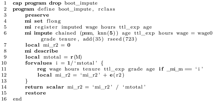
Line 1 clears any older versions of this program from the memory, if already loaded. We start in line 2 by defining the program as r-class, which means that stored results will be returned in r(). Apparently, running the program will change the original data and add new values to the dataset. However, so that the next resampling round can work again on the original dataset, we wrap all operations in preserve/restore to restore any changes made to the data after producing the statistic of interest. The imputation format is set to flong as described above. We register all variables which have missing values as required by Stata. It follows the concrete imputation step where MICE is applied. This model can be as complex as required by your data and research goals. In this demonstration, where all variables in the dataset are continuous, we keep it as simple as possible and use predictive mean matching with five matches each. After the equal sign we list all auxiliary variables that do not contain missing values. The options follow after the comma. We want to generate 35 imputations. We give a random seed so that our results are reproducible. Dots shows the progress of the imputation estimation. This completes the imputation model.
Now all that is left to do is to collect the results. After the imputation has finished, we end up with 35 imputations, which must be combined to arrive at a final result. To do so, we compute the statistic of interest for each imputation and simply form the arithmetic mean of them. An alternative is to compute the median, which is not implemented in this example. We start by defining a local (mi_r2) that will hold our results as we go. We store the total number of imputations in another local (mtotal) and use a loop to go over all imputations separately. The main regression model is estimated, separately for each imputation (which is described with the if-qualifier). Note that this approach only works if the data are imputed in flong. The statistic of interest is added up in the local and finally the mean is computed by diving the sum by the number of imputations. This value is returned in the scalar mi_r2. This concludes the main program.
If we want, we can now run this program on the dataset, which will give us the point estimate of interest. Note that this process contains no randomness (except for the random noise added in the imputation model). To get the bootstrapping results, we can give this program to bootstrap, which conveniently implements all the missing aspects, such as taking random bootstrap samples repeatedly and analyzing the results. This is done as follows:

We open the dataset in Stata and continue with the bootstrap command. We specify that we want to bootstrap the single scalar returned by our program. For testing purposes, only 50 replications are set. We add a random seed and name the main of the command after the colon. Finally, estat gives us desired percentile interval. While this is as simple as it looks, the computational time can be immense. Keep in mind that this specification requires Stata to estimate the imputation model 50 times! You can gauge the approximated runtime by running the program once and measure the time for a single pass, then multiply by the number of desired bootstrap resamples. Keep in mind that a value below 500 might be rather imprecise. To speed things up, you can run the program with parallel to use all system cores [8]. Luckily, doing so is rather simple as well.1
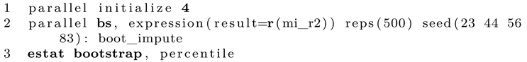
In the first line we set the number of cores to use. This depends on your CPU. The next expression is rather similar to the regular Stata bootstrap command. Note that if you want to set a seed, the number of seeds must be identical to the number of cores specified before.
Impute + Boot
We continue with the approach to impute the data first and only a single time and then apply bootstrapping to this dataset. The advantage is obvious as the potential time-intensive process of imputation has to be done only once and is independent of the bootstrapping itself. The problem is that it is less clear whether the main goal of bootstrapping, that is, randomly and repeatedly resampling from the original data with replacement, is still perfectly valid, since when it is applied after the imputation process where data were generated using the original sample and this only once. However, we want to outline how it can be done in Stata. The algorithm can be summarized as follows.
- Apply your imputation model to the original data to generate M imputed samples and save this newly created dataset.
- To generate the point estimate, run the analytical model separately for each imputed dataset and store the statistics of interests so you get M values. Summarizing these estimates gives the point estimates, which is usually done as the arithmetic mean (an alternative could be the median).
- To compute bootstrap confidence intervals, draw a random bootstrap sample with replacement from the imputed dataset. Here it is crucial that the dependencies within the data are respected. For example, if case number i is selected to be included in the bootstrap sample, it is necessary to include all M datarows for this observation. In the end, for each fo the B bootstrap resamples, M datarows are included.
- For this newly generated bootstrap resample, compute the point estimate as described in step 2.
- Repeat steps 3 and 4 B times to get a collection of bootstrap point estimates (the bootstrap distribution). Compute the percentiles of interest for this collection to receive the confidence interval.
In Stata, this can be done as follows:
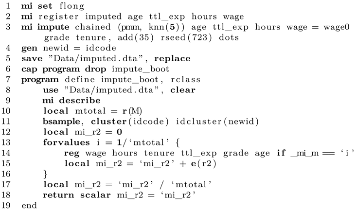
In lines 1 to 3, the data are imputed once as described above. For Stata it is then necessary to create a new ID that first takes the values of the original ID that are, however, later overwritten (line 4). This is necessary if an observation is included multiple times in the bootstrap sample. Suppose observation 6 is drawn two times in total from the original sample, which means that these data are included times. However, it is important that Stata knows that these data rows should be treated as separate observations in the bootstrap sample, so two different IDs will be given, even in the original data are the same. This information is then stored in the new ID, which is called newid in our case. The dataset is then saved to disk.
We continue to write a program that is finally executed many times and accesses the imputed dataset we just stored (line 8). After opening, the number of imputed datasets M is counted and this information stored in a local. Afterwards, a single bootstrap resample is taken with the properties as described above. To achieve this, we tell Stata that the clustering ID is idcode and that the newly created overwritten ID is called newid. After having drawn the bootstrap resample, we can continue to summarize the statistic of interest as already known by running the regression command separately for each imputation version and forming the arithmetic mean over all estimates. This final value is returned by the program in line 18.
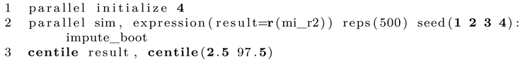
When we run this program, we receive a single bootstrapped point estimate, which is only the first step. To run the program many times, we use Stata’s simulate command. This is a little different from the first approach where we used bootstrap. However, since Stata always needs to start with a fresh copy of the original imputed dataset which is saved to disk, simulate is the way to go here (the bootstrap resampling is done within the program).

Line 1 runs the entire thing. We want to bootstrap the single scalar impute_boot returns, which we call result for convenience. We want 500 simulations and set a seed so the random bootstrap resamples can be reproduced. After the program has finished, Stata automatically opens the results. All we need to to is check the value of percentile 2.5 and 97.5 for a 95% confidence interval, which we can do with centile. Finally, as we have now computed the confidence interval, we need the point estimate. This is done by opening the imputed dataset and running the command of interest a single time, which can be done as follows:
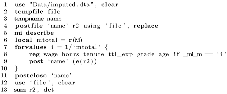
Instead of using a local and summing up individual values, here we show how to use postfile to store each value, which can be interesting for other types of analyses. We set up postfile first and then estimate the statistic of interest separately for each imputation in the dataset. Afterwards, we save the postfile, open it and compute the mean and median of the statistic of interest. Usually, the mean will be reported as the point estimate. Note that in this specification, nothing is saved to disk and only kept in memory. You can either replace tempfile (line 4) with an actual file path on your disk or simply save the computed dataset manually. If desired, we can also run simulate in a parallel fashion as follows:
Just to be clear, some people might wonder why we need to write this extra program instead of giving this task to the Stata bootstrap prefix. One could come up with a solution like this:
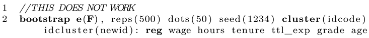
At first, it seems fine since Stata will draw random bootstrap samples and also respect the imputed data structure. However, as you see, reg does not "know" about the imputed data and simply runs over all datapoints in the sample. The higher the number of imputations M, the higher the total case number regress will use. Apparently, this messes up all statistics that depend on sample size, such as standard errors. We could attempt to solve the problem by typing: mi estimate: reg..., however, this commend does not return an R-squared value. A third solution could be to use mibeta from SSC (ssc install mibeta, replace). This would work but only for this very special statistic (R-squared). As long as you write a custom program that sums up the statistic you actually need you are on the safe side as long as Rubin’s rules apply (which is the case for most normally distributed statistics).
Simulation and comparison
By now we have seen how to apply both approaches of bootstrapping imputed data in Stata. Next we want to outline how the different methods perform. Note that this is not a proper simulation approach but only a rather concise demonstration as in-depth review would require many more simulations, which takes a lot of time as the bootstrapping naturally takes a long time to compute a single result. We will compare four different approaches: using the original data without any missings, which is the gold standard and ideal result. Ideally, our imputed results will converge to this result as it is unbiased. Second, listwise deletion is applied without any imputation to test how biased findings can be if nothing is done to combat missing data. Finally, both bootstrap approaches are compared. Evaluated are the point estimates, the distributions of the generated bootstrap statistics and percentiles 2.5 and 97.5 (as these correspond to a 95% confidence interval, which is usually the standard). The following table gives an overview over the simulation specifications (Table 1).
As before, we want to generate a 95% confidence interval for R-squared. The results are shown in the next table (Table 2).
The first and most important thing to notice is that the results for listwise deletion are heavily biased. Since the data are MAR and not MCAR, the resulting R-squared is clearly off. Furthermore, the CI is very wide since the effective sample size is reduced and the uncertainty hence larger. When we look at the imputed approaches we note that the point estimates are identical. This must be the case since the bootstrapping methods are used for inference and not better point estimates. Whether or not to use bootstrapping after imputing your data does not affect the point estimate. We also see that the point estimates are very close to the ideal one which means that our imputation approach is beneficial and is able to account for missing data. This holds since the data is MAR. When looking at the CIs we see that BootImpute performs better than ImputeBoot. For the latter approach, the CI is too narrow. This means that in this kind of interval, the true value is included less often than the expected 95%, resulting in undercoverage. This is a problem if we believe that the nominal coverage should be 95%. However, given that this is a single dataset and a single computation, one should be careful to read too much into these numbers. We continue with a comparison of the resulting bootstrap distributions (Figure 3).
We see that the complete dataset and the BootImpute approach give rather similar distributions of generated statistics (based on 2,000 replications). The distribution for ImputeBoot is a bit too narrow. Completely off is the listwise approach as the distribution is shifted to the right and much too broad. Next we compare the centiles of interest to assess the confidence intervals in more details (Figure 4).
It becomes clear that BootImpute performs very well and is rather close to an ideal result.
References
- Little, R. J., & Rubin, D. B. (2019). Statistical analysis with missing data. John Wiley & Sons.
- Van Buuren, S. (2018). Flexible imputation of missing data. CRC press.
- Bittmann, F. (2021). Bootstrapping: an integrated approach with Python and Stata. Walter de Gruyter GmbH & Co KG.
- Efron, B., & Tibshirani, R. J. (1994). An introduction to the bootstrap. CRC press.
- Bittmann, F. (2019). Stata: A really short introduction. Walter de Gruyter GmbH & Co KG.
- Hesterberg, T. C. What teachers should know about the bootstrap: Resampling in the undergraduate statistics curriculum. The American Statistician 2015, 69, 371–386. [Google Scholar] [CrossRef] [PubMed]
- Schomaker, M., & Heumann, C. Bootstrap inference when using multiple imputation. Statistics in medicine 2018, 37(14), 2252–2266. [PubMed]
- Vega Yon, G. G., & Quistorff, B. parallel: A command for parallel computing. The Stata Journal 2019, 19, 667–684.
| 1 | First, you need to install parallel from the Github repository (https://github.com/gvegayon/parallel). Follow the manual and restart Stata afterwards. |
Figure 1.
Stata output.
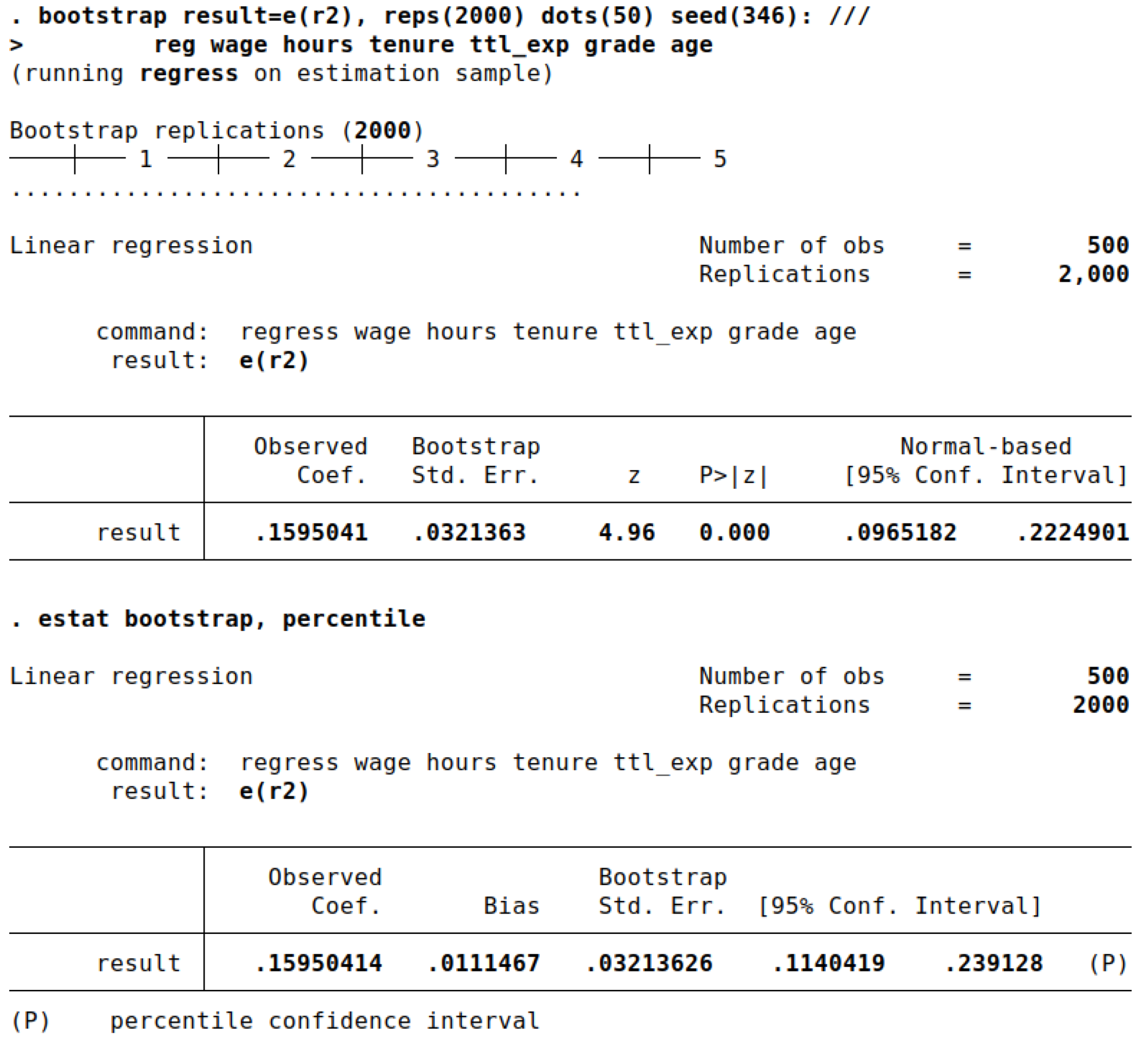
Figure 2.
Data format flong in Stata (imputed dataset).
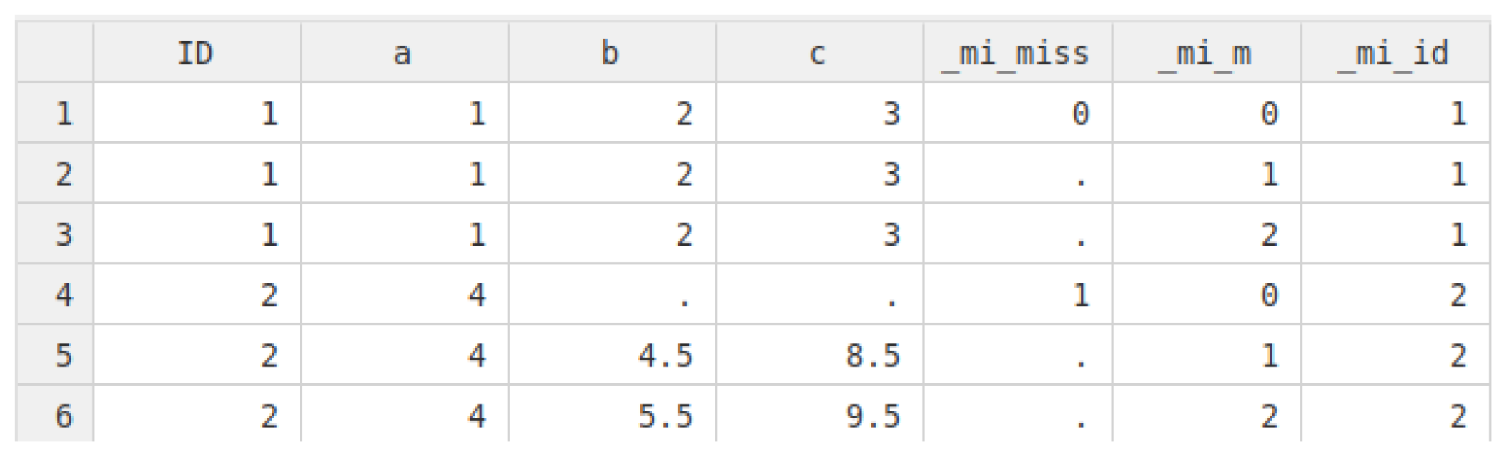
Figure 3.
Comparison of bootstrap distributions by approach.
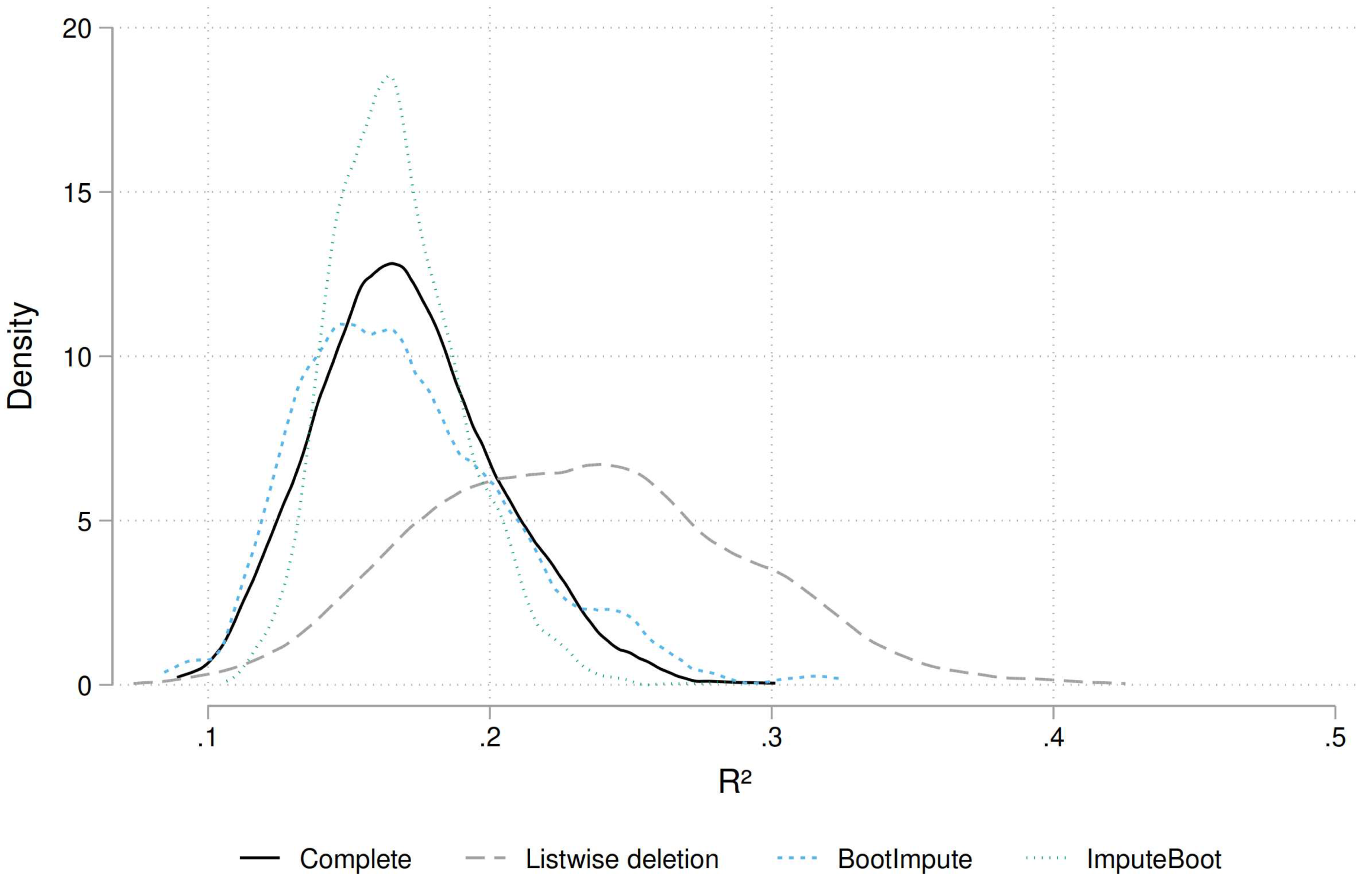
Figure 4.
Quantiles 2.5 and 97.5 of the generated bootstrap distributions by approach, including 95% CIs. The dashed horizontal line indicates the ideal result.
Figure 4.
Quantiles 2.5 and 97.5 of the generated bootstrap distributions by approach, including 95% CIs. The dashed horizontal line indicates the ideal result.
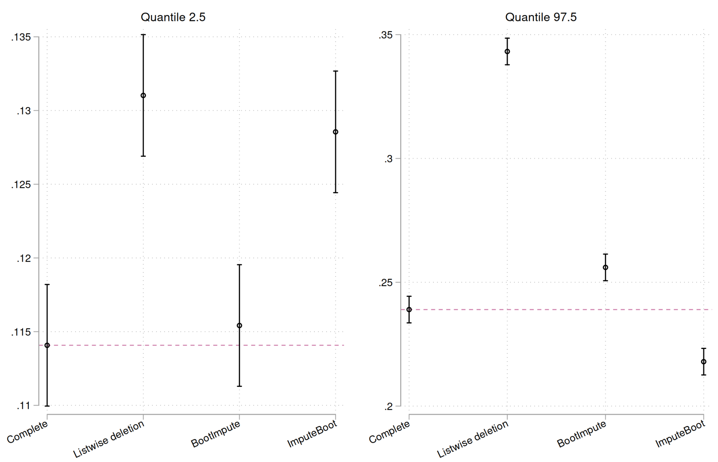

Table 1.
Simulation specifications.
| Approach | Bootstrap Resamples | Number of imputations |
| Complete data | 2000 | - |
| Listwise deletion | 2000 | - |
| Boot + Impute | 2000 | 35 (per bootstrap resample) |
| Impute + Boot | 2000 | 35 (impute dataset once) |
Table 2.
Resulting point estimates and CIs by approach.
| Approach | Point estimate (R²) | 95% CI |
|---|---|---|
| Complete data | 15.95 | 11.40; 23.91 |
| Listwise deletion | 21.13 | 13.16; 34.30 |
| Boot + Impute | 15.75 | 11.57; 25.59 |
| Impute + Boot | 15.75 | 12.86; 21.79 |
Disclaimer/Publisher’s Note: The statements, opinions and data contained in all publications are solely those of the individual author(s) and contributor(s) and not of MDPI and/or the editor(s). MDPI and/or the editor(s) disclaim responsibility for any injury to people or property resulting from any ideas, methods, instructions or products referred to in the content. |
© 2024 by the authors. Licensee MDPI, Basel, Switzerland. This article is an open access article distributed under the terms and conditions of the Creative Commons Attribution (CC BY) license (http://creativecommons.org/licenses/by/4.0/).
Copyright: This open access article is published under a Creative Commons CC BY 4.0 license, which permit the free download, distribution, and reuse, provided that the author and preprint are cited in any reuse.


