1. Introduction
The increased incorporation of renewable energy systems (RES) in the world energy system, replacing traditional thermal power stations, has been translated into important advantages in the reduction of atmospheric pollutants. Concerning the building sector, residential end users are moving from simple energy consumers to active prosumers (i.e., those who consume and produce energy), proactively managing their energy demands through energy production systems and, in some cases, using energy storage systems, such as battery energy storage (ES), and/or electric vehicles (EVs). Surplus electricity can be, in most cases, traded with grid companies.
This completely decentralized approach, however, has also disadvantages. From the grid point of view, it can introduce instability, resulting in increased interactions and unpredictable fluctuations; from the prosumers point of view, it is not so beneficial as expected, since generally, there is a large difference between buying and selling electricity tariffs. Due to these reasons, the concept of sharing and exchanging electricity between prosumers has emerged as a promising solution for achieving collective benefits. Energy communities, made up of interconnected loads and distributed energy resources (DERs), can employ energy management strategies that maximize community self-consumption and reduce dependence on the central grid. Different energy sharing strategies are discussed in [
1], where it is assumed that each community member has an intelligent home energy management system (HEMS) managing its own flow of energy, under the supervision of an intelligent aggregator which controls the whole energy community and being also responsible for the community’s interaction with the central grid.
Nowadays, in many countries all over the world, the production and sale of electricity is traded under competitive rules in free markets. Thus, the electricity demand and price forecasting are a main target for the agents and companies involved in the electricity markets. In particular, short-term forecast, which is the one day ahead hourly forecast, has been extensively studied in the literature. Excellent reviews on demand and price forecasting can be found in [
2,
3] and [
4,
5], respectively. Works on load demand and price forecasts for several energy markets can be found in [
6], for the Spanish market in [
7] and for Portuguese energy market in [
8].
This paper assumes the scenario of a community of energy managed by an aggregator. Additionally, it is also considered that the aggregator will buy the electricity needed by the community in an energy market, such as the Iberian Electricity Market – MIBEL. The day-ahead market of MIBEL is the platform where electricity is transacted for delivery on the day after the negotiation. This market is priced for each of the 24 hours of each day and for each one of the 365 or 366 days of each year. Every day the daily market platform is active until 12:00, when, at the close of the session, electricity prices are presented for the following day. Before this deadline, the energy proposals of purchase and sale are made, which will be in the origin of the value of the prices of electricity for each day-ahead hour.
To efficiently manage the community, the aggregator needs to employ good forecasts of the day-ahead net energy or power required, as well as the future selling/buying prices. This paper will deal only with the day-ahead net power and will assume that day-ahead prices are obtained by other techniques. As the net power is the difference between the load demand and the electricity produced, good forecasts of both variables are required. In addition, if the aggregator manages different communities of energy, these forecasts should be extended to the aggregation of all day-ahead net energy foreseen.
The existing load and generation forecast can be classified in terms of forecasting results into two categories: point forecast and probabilistic forecast [
9]. Traditional point forecasting provides a single accurate estimate for future power, which is unable to adequately quantify the uncertainty associated with the actual variable. On the other hand, probabilistic forecasting is receiving considerable research attention due to its superior ability of capturing future demand uncertainty. Probabilistic prediction can better describe the uncertain components contained in the deterministic prediction results in three forms: prediction intervals (PI), quantile, and probability density function (PDF) [
10]. The forecasting methods based on PIs are trained by optimizing the error-based loss function, and the output of the trained prediction model is used to construct PIs [
11]. Traditional PI methods, such as Bayesian [
12], Delta [
13], Bootstrap [
14] and mean-variance (MVE) [
15] construct the corresponding PIs sequentially. In this paper, we shall be using the covariance method, introduced in [
16] and discussed later on.
Specifically for load demand point forecasting, the works [17-19] can be highlighted. In the former, data from four residential buildings, sampled with an interval of 15 minutes, is employed. Three forecasting models are compared: i) the Persistence-based Auto-regressive model, ii) the Seasonal Persistence-based Regressive model, and iii) the Seasonal Persistence-based Neural Network model, as well as mixtures of these three methods.
Kiprijanovska and others [
18] propose for forecasting a deep residual neural network, which integrates multiple sources of information by extracting features from (i) contextual data (weather, calendar), and (ii) the historical load of the particular household and all households present in the dataset. Authors compared their approach with other techniques on 925 households of Pecan Street database [
20] with data re-sampled at 1 hour time interval. Day-ahead forecasts are computed at 10 hours, the previous day. The proposed approach achieves excellent results, in terms of RMSE, MAE and R
2.
Pirbazari and co-authors [
19] employed hourly data from a public set of 300 Australian houses, available from 2010 to 2013. This set consisted of load demand and electricity generation for the six hundred houses, which have, for analysis, been divided into 6 different 50 houses groups. For forecasting, they propose a predicting approach that first considers the highly influential factors and, second, benefits from an ensemble learning method where one Gradient Boosted Regression Tree algorithm is combined with several Sequence-to-Sequence Long Short-Time Memory (LSTM) networks. The ensemble technique obtained the best 24-hours ahead results, for both load and generation, when compared to other isolated and ensemble approaches.
Focusing now on PV generation point forecasting, the work [
21] should be mentioned. The authors propose a LSTM-attention-embedding model based on Bayesian optimization to predict the day-ahead PV power output. The effectiveness of the proposed model is verified on two actual PV power plants in one area of China. The comparative experimental results show that the performance of the proposed model has been significantly improved compared to LSTM neural networks, Back-Propagation Neural Networks (BPNN), Support Vector Regression machines (SVR) and persistence models.
The works cited above deal with point forecasting. We shall now move to a probabilistic forecasting survey.
Jaun Vilar et. al. [
6] proposes two procedures to obtain prediction intervals for electricity demand (as well as price) based on functional data. The proposed procedures are related to one day ahead pointwise forecast. The first method uses a nonparametric autoregressive model and the second one uses a partial linear semi-parametric model, in which exogenous scalar covariates are incorporated in a linear way. In both cases, the proposed procedures for the construction of the prediction intervals use residual-based bootstrap algorithms, which allows also to obtain estimates of the prediction density. The 2012 entire year of the total load demand in Spain is employed, using a hourly sampling time. It has been found that, using the Winkler score, the second method obtains better results.
Zhang and co-workers [
9] propose a probability density prediction method based on monotone composite quantile regression neural network and Gaussian kernel function (MCQRNNG) for day-ahead load. Taking real load data carrying quantile crossing from Ottawa in Canada, Baden-Württemberg in Germany and a certain region in China, the performance of the MCQRNNG model is verified from three aspects: point, interval, and probability prediction. Results show that the proposed model significantly outperforms the comparison model based on effectively extricating the quantile crossing for power load forecasting.
Regarding PV generation, [
22,
23] should be mentioned. The former compares the suitability of a non-parametric and three parametric distributions in the characterization of prediction intervals of photovoltaic power forecasts with high confidence levels. The calculations were done for one year of day-ahead forecasts of hourly power generation of 432 PV systems. The results showed that, in general, the non-parametric distribution assumption for the forecast error yielded the best prediction intervals.
Mei et. al. [
23] propose an LSTM- Quantile Regression Averaging (QRA)-based nonparametric probabilistic forecasting model for PV output power. A set of independent LSTM deterministic forecasting models is trained using historical PV data and Numerical Weather Prediction (NWP) data. Nonparametric probabilistic forecasting is generated by integrating the independent LSTM prediction models with Quantile Regression Averaging (QRA). In comparison with the benchmark methods, LSTM-QRA has higher prediction performance due to the better forecasting accuracy of independent deterministic forecasts.
Finally, [
24] seems to be the only publication looking at the net load forecasting of residential microgrids. The authors propose a data-driven-based net load uncertainty quantification fusion mechanisms for cloud-based energy storage management with renewable energy integration. Firstly, a fusion model is developed using SVR, LSTM, and Convolutional Neural Network – Gated Recurrent Unit (CNN-GRU) algorithms to estimate day-ahead load and PV power forecasting errors. After that, two mechanisms are proposed to determine the day-ahead net load error. In the first mechanism, the net load error is directly forecasted, while in the second mechanism, it is derived from the forecast errors of load and PV power. The uncertainty is analyzed with various probability confidence intervals. However, those are not prediction intervals and, this way, the actual data does not lie within those bounds. Additionally, the forecasts are computed in the end of one day for the next 24 hours, i.e., the PH is only of 24 hours and cannot be used for energy markets.
The present paper solves the issues mentioned in relation with the last reference. It allows to obtain, for the community(s) managed an aggregator, excellent day-ahead hourly point forecasts of the net load, whose robustness can be accessed by prediction intervals obtained at a user-specified confidence level. This allows the aggregator to make more informed decisions regarding energy buying (and or selling).
This is achieved by the use of robust ensemble forecasting models, which will be described in
Section 2. The data employed and the results obtained are presented in
Section 3. They are discussed in
Section 4 and compared with results obtained by other works.
Section 5 concludes the paper.
2. Material and Methods
The design of robust ensemble forecasting models has been discussed elsewhere (please see [
25]) and will only be summarized here.
To obtain “good” single models from a set of acquired or existent data, three sub-steps must be followed:
data selection – this is a pre-processing stage where, from the existing data, suitable sets (training, testing, validation, …) must be constructed.
features/delays selection - given the above data sets, the “best” set of inputs and network topology should be determined.
parameter estimation - given the data sets constructed and using the inputs/delays and network topology chosen, the “best” network parameters should be determined.
These are solved by the application of a model design framework, composed of two existing tools. The first, denoted as ApproxHull, performs data selection, from the data available for design. Feature and topology search are obtained by the evolutionary part of MOGA (Multi-Objective Genetic Algorithm), while parameter estimation is performed by the gradient part of MOGA.
2.1. Data Selection
To design data driven models it is mandatory that the samples that enclose the whole input-output range where the underlying process is supposed to operate should be present in the training set. To determine such samples, called convex hull (CH) points, out of the whole dataset, convex hull algorithms can be applied.
As standard convex hull algorithms suffer from both exaggerated time and space complexity for high dimensions, a randomized approximation convex hull algorithm, denoted as ApproxHull, proposed in [
26], is employed.
In a prior step before determining the CH points, ApproxHull eliminates replicas and linear combinations of samples/features. After having identified the CH points, ApproxHull generates the training, test and validation sets to be used by MOGA, according to user-specifications, but incorporating mandatorily the CH points in the training set.
2.2. MOGA
This framework is described in detail in [
27], and it will be briefly discussed here.
MOGA designs static or dynamic ANN (Artificial Neural Network) models, for classification, approximation or forecasting purposes.
2.2.1. Parameter Separability
MOGA employes models that are linear-nonlinearly separable in the parameters [
28]. The output of this type of models, at sample
k, is given as:
In (1),
is the
kth input sample,
φ is the basis functions vector,
u is the (linear) output weights vector and
v represents the nonlinear parameters. For simplicity, we shall assume here only one hidden layer, and this way
v is composed of
n vectors of parameters, each one for each neuron
. This type of models comprises Multilayer Perceptrons, Radial Basis Function (RBF) networks, B-Spline and Asmod models, Wavelet networks, and Mamdani, Takagi and Takagi-Sugeno fuzzy models (satisfying certain assumptions) [
29].
In the case described here, RBF models will be employed. The basis functions employed by RBFs are typically Gaussian functions:
Which means that the nonlinear parameters for each neuron are constituted by a centre vector, , with as many components as the dimensions of the input, and a spread parameter, σi.
Associated with each model, there are always heuristics that can be used to obtain the initial values of the parameters. For RBFs, centre values can be obtained randomly from the input data, or from the range of the input data. Alternatively, clustering algorithms can be employed. Initial spreads can be chosen randomly, or using several heuristics, such as:
where
zmax represents the maximum distance between centres and
n represents the number of neurons.
For the general case, the model parameters can this way be divided into linear (
u) and nonlinear (
v) parameters:
and this separability can be exploited in the training algorithms. For a set of input patterns
X, training the model means finding the values of
w, such that the following criterion is minimized:
where y is the target vector,
is the RBF output vector, and ||.||
2 denotes the Euclidean norm. Replacing (1) in (5), we have:
Where
,
m being the number of patterns in the training set. As (4) is a linear problem in
u, its global optimal solution is given as:
Where the symbol ‘+’ denotes a pseudo-inverse operation. Replacing (7) in (6), we have a new criterion, which is only dependent on the nonlinear parameters,
v:
2.2.2. Training Algorithm
Any gradient algorithm can be used to minimize (6) or (8). For non-linear least-squares problems, the Levenberg-Marquardt (LM) method [
30,
31] is recognized to be the state-of-the-art method, as it exploits the sum-of-squares characteristics of the problem. The LM search direction at iteration
k (
is given as the solution of:
where
is the gradient vector:
and
is the Jacobean matrix:
The parameter λ is a regularization parameter, which enables the search direction to change between the steepest descent and the Gauss-Newton directions. The gradient and Jacobean of criterion (8) can be obtained by: a) first computing (7); b) replacing the optimal values in the linear parameters; c) and determining the gradient and Jacobian in the usual way.
In MOGA, the training algorithm terminates after a predefined number of iterations, or using an early-stopping technique [
32].
2.2.3. The evolutionary part
MOGA evolves ANN (in the case of the present paper, RBFs) structures, whose parameters separate, each structure being trained by the LM algorithm minimizing (8). We shall be using multi-step-ahead forecasting, and this way each model should be iterated
PH times to predict the evolution of a variable within a selected Prediction Horizon (
PH). For each step, the model inputs evolve with time. Consider the Nonlinear Auto-Regressive model with Exogeneous inputs (NARX), with just one input,
x, for simplicity:
Where denotes the prediction for time-step k+1 given the measured data at time k, and the jth delay for variable k. This represents the 1-step-ahead prediction within a prediction horizon. As (12) is iterated over PH, some or all the indices in the right hand-side of (12) will be larger than j, which means that there are no measured values, and the corresponding forecast must be employed. What has been said for NARX models is also valid for NAR models (models with no exogeneous inputs).
The evolutionary part of MOGA evolves a population of ANN structures. Each topology consists of the number of neurons in the single hidden layer (for an RBF model), and the model inputs or features. MOGA assumes that the number of neurons must be within a user-specified bound, n ∈ [nm, nM]. Additionally, one needs to select the features to use for a specific model, i.e., input selection must be performed. In MOGA it is assumed that, from a total number q of available features, denoted as F, each model must select the most representative d features within a user-specified interval, d ∈ [dm, dM], dM ≤ q, dm representing the minimum number of features, and dM its maximum number.
The operation of MOGA is a typical evolutionary procedure, with the operators conveniently changed to implement topology and feature selection. We shall refer the reader to publication [
27] regarding a more detailed explanation of MOGA.
MOGA is a multi-objective optimizer which means that the optimization objectives and goals need to be defined. Typical objectives are Root-Mean-Square Errors (RMSE) evaluated on the training set (
ρtr), or on the test set (
ρte), as well as the model complexity, #(
v) - number of nonlinear parameters - or the norm of the linear parameters (||
u||
2). For forecasting applications one criterion is also used to assess its performance. Assuming a time-series
sim, a subset of the design data, with
p data points is considered. For each point, the model (11) is used to make predictions up to
PH steps-ahead. Then an error matrix is built:
where
e[
i,
j] is the model forecasting error taken from instant
i of
sim, at step
j within the prediction horizon. Denoting the RMS function operating over the
ith column of matrix
E, by
, the forecasting performance criterion is the sum of the RMS of the columns of
E:
Notice that in the MOGA formulation every performance criterion can be minimized or set as a restriction to be met.
After having formulated the optimization problem, and after setting other hyperparameters, such as the number of elements in the population (npop), number of iterations population (niter), and genetic algorithm parameters (proportion of random immigrants, selective pressure, crossover rate and survival rate), the hybrid evolutive-gradient method is executed.
Each element in the population corresponds to a certain RBF structure. As the model is nonlinear, a gradient algorithm such as the LM algorithm minimizing (6) is only guaranteed to converge to a local minimum. For this reason, the RBF model is trained a user-specified number of times, starting with different initial values for the nonlinear parameters. MOGA allows initial centers chosen from the heuristics mentioned in
Section 2.2.1, or using an adaptive clustering algorithm [
33].
After having executed the specified number of iterations, we have performance values of npop * niter different models. As the problem is multi-objective, a subset of these models corresponds to non-dominated models (nd), or Pareto solutions. If one or more objectives is (are) set as restriction(s), then a subset of nd, denoted as preferential solutions, pref, corresponds to the non-dominated solutions that met the goals.
The performance of MOGA models is assessed on the non-dominated models set, or in the preferential models set. If a single solution is sought, it will be chosen based on the objective values of those model sets, of performance criteria applied to the validation set, and possibly other criteria.
When the analysis of the solutions provided by the MOGA requires the process to be repeated, the problem definition steps should be revised. In this case, two major actions can be conducted: input space redefinition by removing or adding one or more features (variables and lagged input terms in the case of forecasting problems) and improving the trade-off surface coverage by changing objectives or redefining goals. This results in a smaller search space in a subsequent run of the MOGA, possibly achieving a faster convergence and better approximation of the Pareto front.
Typically, for a specific problem, an initial MOGA execution is performed, minimizing all objectives. Then a second execution is run, where typically some objectives are set as restrictions.
2.3. Model Ensemble
According to the previous discussion the output of MOGA is not a single model, but sets of nondominated RBFs or, possibly, preferential models. The models within these sets are typically powerful models, all with a different structure, which can be used to form a stacking ensemble.
Several combination approaches have been applied for ensemble models. The most usual way is the use of the mean, against which other alternatives are compared. The authors of [
34] propose four approaches: the median, the use of weights proportional to the probability of success, the use of weights calculated by variance minimization, and the use of weights calculated from eigenvector of covariance matrix of forecast errors. Other alternatives are even more complex. For instance, in [
35] a Bayesian combination approach for combining ANN and linear regression predictor has been used. In [
36] a combination of weather forecasts from different sources using aggregated forecast from exponential reweighting is proposed.
To be employed in computationally intensive tasks, a computationally simple technique of combining the outputs of the model ensemble must be employed. As in a few exceptional cases, MOGA-generated models have been found with outputs that can be considered as outliers, the ensemble output is obtained as a
median, and not as a mean. The ensemble output model, using a set of models, denoted as
outset, is therefore given as:
n being the number of elements of
outset. It was argued in [
25] that 25 was a convenient number of elements for outset, and its elements should be selected using a Pareto concept. Specifically, the following sequence of procedures should be followed for model design:
- i)
Use ApproxHull to select the datasets from the available design data.
- ii)
Formulate MOGA, in a first step, minimizing the different objectives.
- iii)
Analyze MOGA results, restrict some objectives and redefine input space and/or the model topology.
- iv)
Use the preferential set of models obtained from the second MOGA execution for the next steps.
- v)
Determine
using
Where
,
,
is the set of preferential models obtained in the 2
nd MOGA execution,
is the set of the linear weight norm for each model in
,
being its median;
is the set of the sum of the forecasts for the prediction time-series obtained for all models in
, computed using (15), being
its median.
- vi)
-
From
obtain
using:
This set is obtained iteratively, by adding non-dominated models, considering nw(.) and fore(.) as the two criteria, until 25 models are found. Initially, the set of models to be inspected, is initialized to , and to an empty set. In each iteration, both criteria are applied to . Then, the non-dominated solutions found are added to and removed from .
- vii)
If the model that should be designed is a NARX model, use for the exogenous variables.
2.4. Robust Models
Recent inclusion of smart grids and renewable integration requirements induced the drawback of increasing the uncertainty of future prices, supply and demand. Academics and practitioners alike realized that probabilistic electricity price, load and production forecasting is now more important for energy systems planning and operations than ever before [
37,
38].
Predictive modeling assumes that all observations are generated by a data generating function
f(
x) combined with additive noise:
where
is the point forecast of the variable at time
k obtained using data available at an earlier point in time and is a data noise term, responsible for introducing uncertainty in the model. This can be decomposed into three terms:
training data uncertainty, related with the uncertainty over how representative is the training data with respect to the whole operational range of the model input;
model misspecification, related with the fact that the model, with its optimal parameters and data conditions, can only approximate the real underlying function generating the data; and
parameter uncertainty, related with the fact that the parameters employed in the model might not be the optimal ones. Notice that ApproxHull tries to minimize the first type of uncertainty, the evolutionary part of MOGA the second one and the derivative part of MOGA minimizes the third one.
The most common extension from point to probabilistic forecasts is to construct prediction intervals (PIs). A number of methods can be used for this purpose, the most popular consider both the point forecast and the corresponding error. A (1 − α) PI implies that the interval contains the true value with a probability of (1 − α). Transferring this idea to the calculation of quantiles leads to τ = α/2 lower bound and τ = (1 – α/2) for the upper bound [
39]. For instance, we need to calculate the 5% and 95% quantiles to yield a 90% PI if the distance between the two quantiles is considered, which is the level used in this paper. We will denote as
and
the upper and lower bounds, respectively.
There are diverse ways to compute the PIs. The interested reader can consult [
11], which describes different possibilities. In this case the covariance method introduced in [
16] is employed. Using the notation
, introduced before to denote the output matrix of the last nonlinear layer, which is dependent on the input matrix,
X, and on the nonlinear parameters
v. The total prediction variance for each prediction
can therefore be obtained as
where
Ztr is the input training matrix, and the data noise variance,
, can be estimated as:
where
N denotes the total number of samples and
p the number of model parameters. The bounds are assumed to be symmetric and given as:
where represents the α/2 quantile of a Student’s t-distribution with
N −
p degrees of freedom.
In particular, we can use in (18) the optimal parameter values obtained after training, and . Notice that, due to the training of the model in MOGA, we have available (or can indirectly be obtained) these two quantities, if belongs either to the test or validations sets. In other words, it is not computationally expensive to compute (18).
2.5. Robust Ensemble Forecasting models
For every time instant k, we are interested in determining PH forecasts , together with the corresponding bounds .
As we are dealing with an ensemble of models, and using the notation introduced in (15), we shall denote the forecasts as to signify that, at each step, we shall be using the median value of the ensemble of values, computed using (15).
In the same way, the corresponding bound will be denoted as
and
and
in (18) will be denoted as
and
. Therefore, (19-22) should be replaced by:
2.6. Performance criteria
To assess the quality of the models, both in terms of robustness and in terms of the quality of approximation, different criteria will be used.
In this paper the following criteria of assessing the approximation quality will be employed: Root-Mean-Square of the Errors (
RMSE) (27), Mean-Absolute Error (
MAE) (28), Mean-Absolute Percentage Error (
MAPE) (29) and Coefficient of Determination or R-Square (
R2) (30). As we would like to assess the performance of the estimation not only for the next time-ahead, but along
PH, all the different indices will be averaged over the Prediction Horizon. For all indices,
N is the number of samples considered.
Related with robustness of the solutions, some measures have been proposed. One of the simplest is the Average Width (AW):
Where the width is given as:
In (32), and are the upper and lower bounds, introduced in (25), of the model output for time k+s, given the data available until time k, respectively.
A more sophisticated measure of interval width is the Prediction Interval Normalized Averaged Width (PINAW), defined as:
where
R is the range of the whole prediction set:
On the other hand, if we are interested in the magnitude of the violations, we can use the Interval-based Mean Error (IME), also called the PI Normalized Average Deviation (PINAD):
To assess the coverage, we can use the Prediction Interval Coverage Probability (PICP). PICP indicates if the interval given by the bounds
contains the real measure of
:
where
Another metric that is often used to assess both the reliability and the sharpness of the PIs is the Winkler Score [
40]. As it can be seen, it penalizes the interval width with the magnitude of the violations, weighted proportionally by the confidence level.
As we would like to assess the robustness of the estimation not only for one time-ahead, but along
PH, all these criteria must be averaged over
PH.
3. Results
3.1. The Data
Data acquired from a community of energy situated Algarve, Portugal, from two time-periods, were used. Although much smaller sampling intervals were used, the data has been down sampled to intervals of one hour. The first period contained data from the 30th November 2021 to the 17th March 2022 (2583 samples), and the second period comprised data from 22 March 2022 to 3 Jun 2022 (1762 samples). The houses and the data acquisition system are described in [
41,
42], and the reader is encouraged to consult these references. The data used here can be freely downloaded at [
43].
The data that will be used here is weather data, atmospheric air temperature (
T) and global solar radiation (
R), Power Demand (
PD) and PV Power generated (
PG) Additional data that is going to be used is a codification for the type of day (
DE). This characterizes each day of the week and the occurrence and severity of holidays based on the day they occur, as may be consulted in [
8,
44]. In
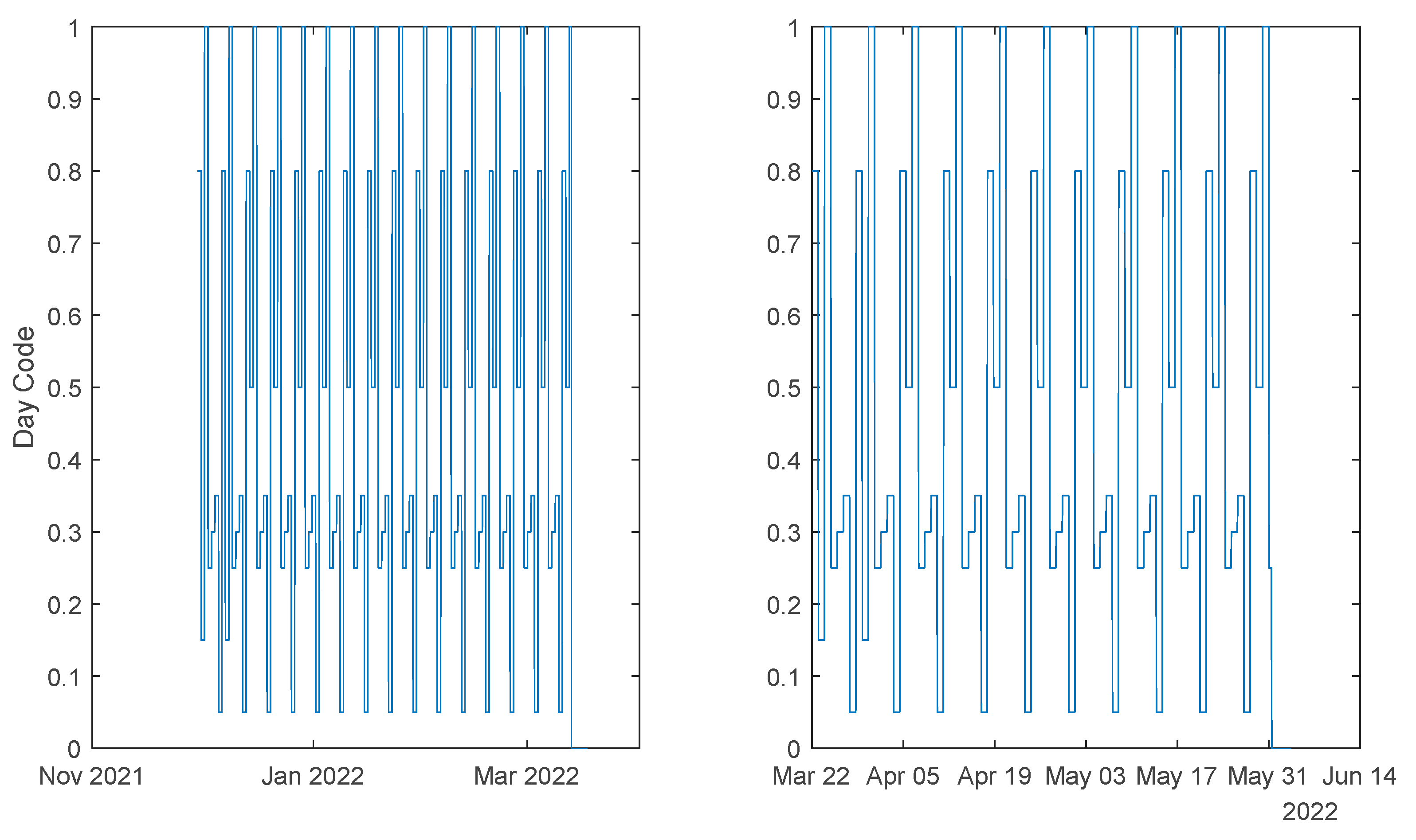
Table 1, the regular day column shows the coding for the days of the week when these are not a holiday. The following column presents the values encoded when there is a holiday, and finally, the special column shows the values that substitute the regular day value in two special cases: for Mondays when Tuesday is a holiday and for Fridays when Thursday is a holiday.
To be able to help the aggregator regarding the needs of purchasing/selling electricity from/to the market, in the sample related to the period between 11h-12h each day, there is the need to forecast the future community power demand and power generated related with next day, i.e., from 0 to 24 hour, in a 1-hour intervals. The former can be modelled as an ensemble of NARX models, for house
h:
The use of the overline symbol in the last equation denotes a set of delayed values of the corresponding variable. As four houses will be considered in the community, four different ensemble models can be used, and the summation of their outputs used to determine the predictive power demand of the community:
An alternative is to employ only one ensemble model, with the sum of the four demands:
The power generated can also be modelled as a NARX model:
As it can be seen (46) and (48) use as exogeneous variables the air temperature and (49) the air temperature and the solar radiation. This means that the evolution of these variables should be predicted. The solar radiation can be modelled as an ensemble of NAR models:
while the air temperature is modelled as:
As described earlier, several models will be designed: four power demand models, one for each house, and an additional one for the community; two weather models and one power generated model. The procedure described
Section 2.2 and detailed in [
25] is followed, and will be briefly summarized here. For each model, two executions of MOGA were performed, the first only minimizing four objectives,
ρtr,
ρte, #(
v) and
ρsim(PH), and in the second execution some objectives are set as goals.
For all problems, MOGA was parameterized with the following values:
Prediction Horizon: thirty-six steps (36 h).
Number of neuros: ;
Initial parameter values:
OAKM [
33];
Number of training trials: five, best compromise solution.
Termination criterion: early stopping, with a maximum number of iterations of fifty.
Number of generations: 100.
Population size: 100.
Proportion of random emigrants: 0.10.
Crossover rate: 0.70.
As already mentioned, for each model, two executions of MOGA are performed, the results of the first being analyzed to constrain the objectives, and ranges of neurons and inputs of the second execution.
For the NARX models, the number of admissible inputs ranged from 1 to 30, while for the NAR model the range employed was from 1 to 20.
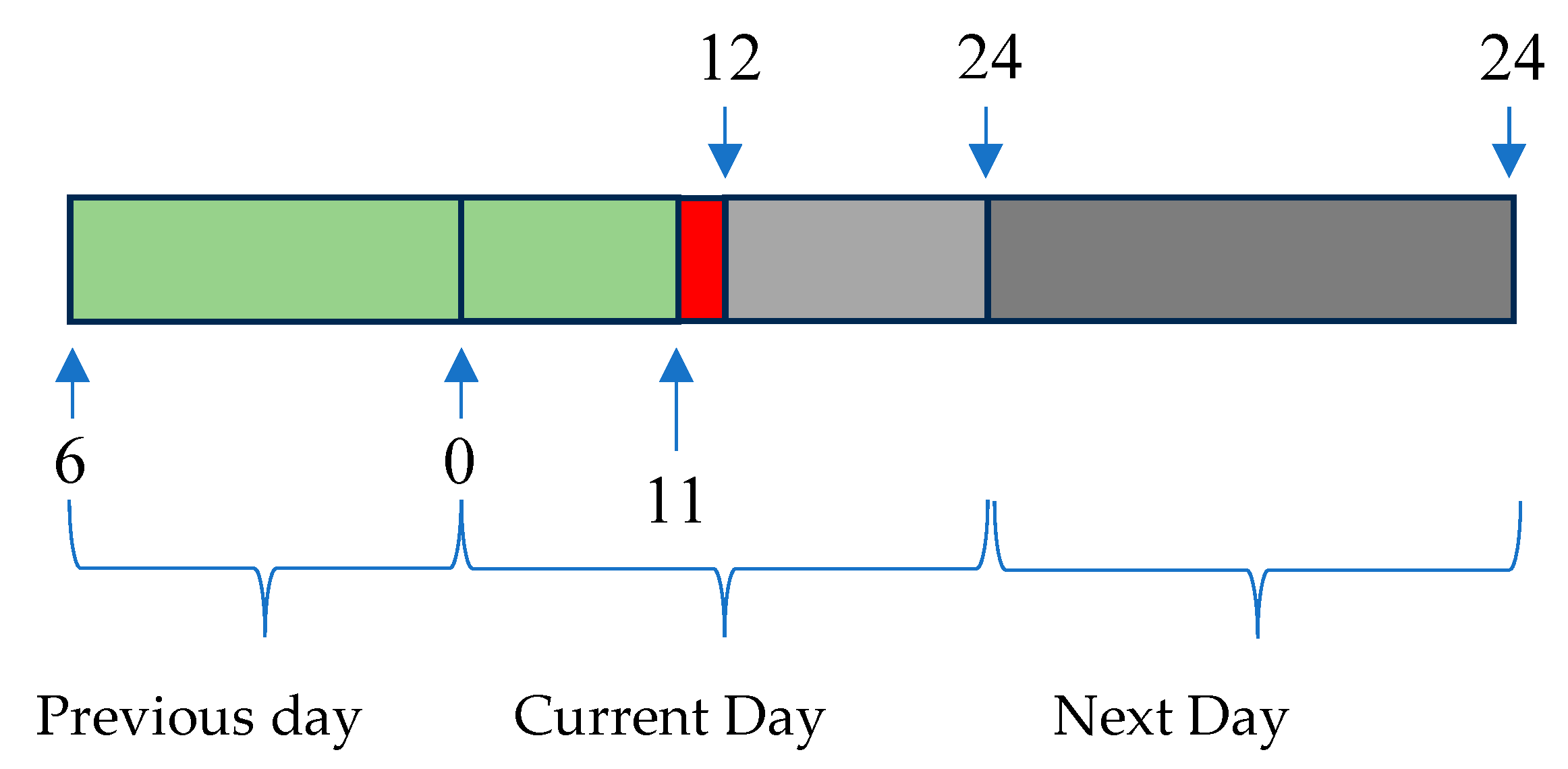
The next figure illustrates the range of forecasts pretended and the delays employed. Every day, a few minutes before 12, the average power for the period 11-12 is computed. Let us denote the index of this sample by k (in red). Using the delayed average powers of the previous 29 indices [k-1 ... k-29] (shown in green), we need to forecast the average powers for next day. Therefore, using a multi-step forecast model, there is the need to forecast 36 steps-ahead values (in cyan), from which only the last 24 steps are required (darker cyan).
The forecasting performance will be assessed using a prediction time-series, from 19-Jan-2022 00:30:00, to 25-Jan-2022 23:30:00, with 168 samples.
3.2. Solar Radiation models
Solar Radiation is a NAR model.
Table 2 shows statistics, corresponding to the mean of the employed performance criteria, averaged over the Prediction Horizon. For this model and for the others, the results are related with the 2
nd MOGA execution. Unless explicitly specified, scaled values, belonging to the interval [-1 … 1] are employed. This enables a comparison of the performance between different variables. The MAPE value shown is in %.
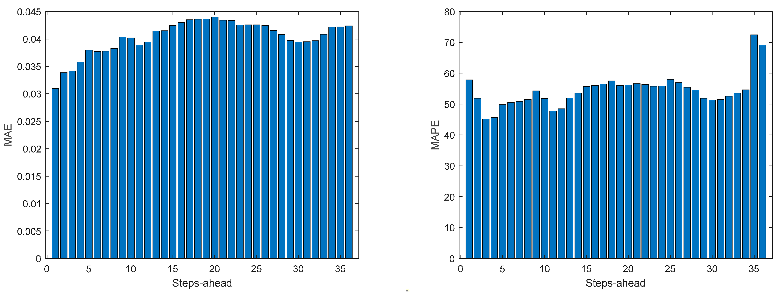
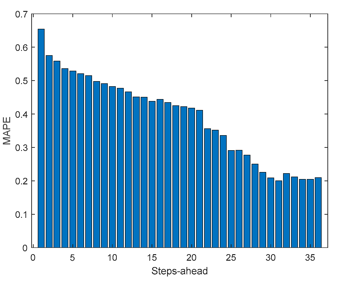
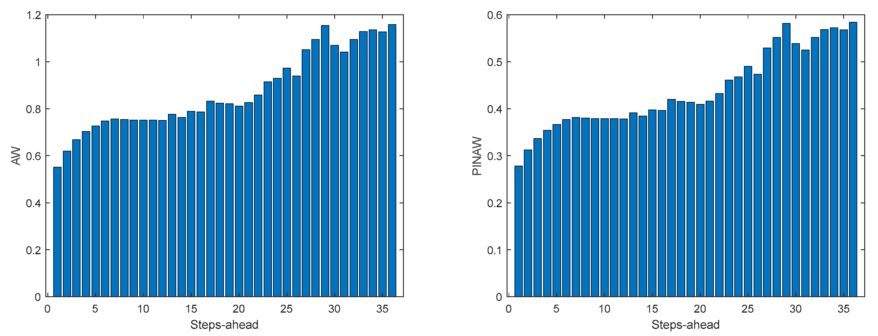
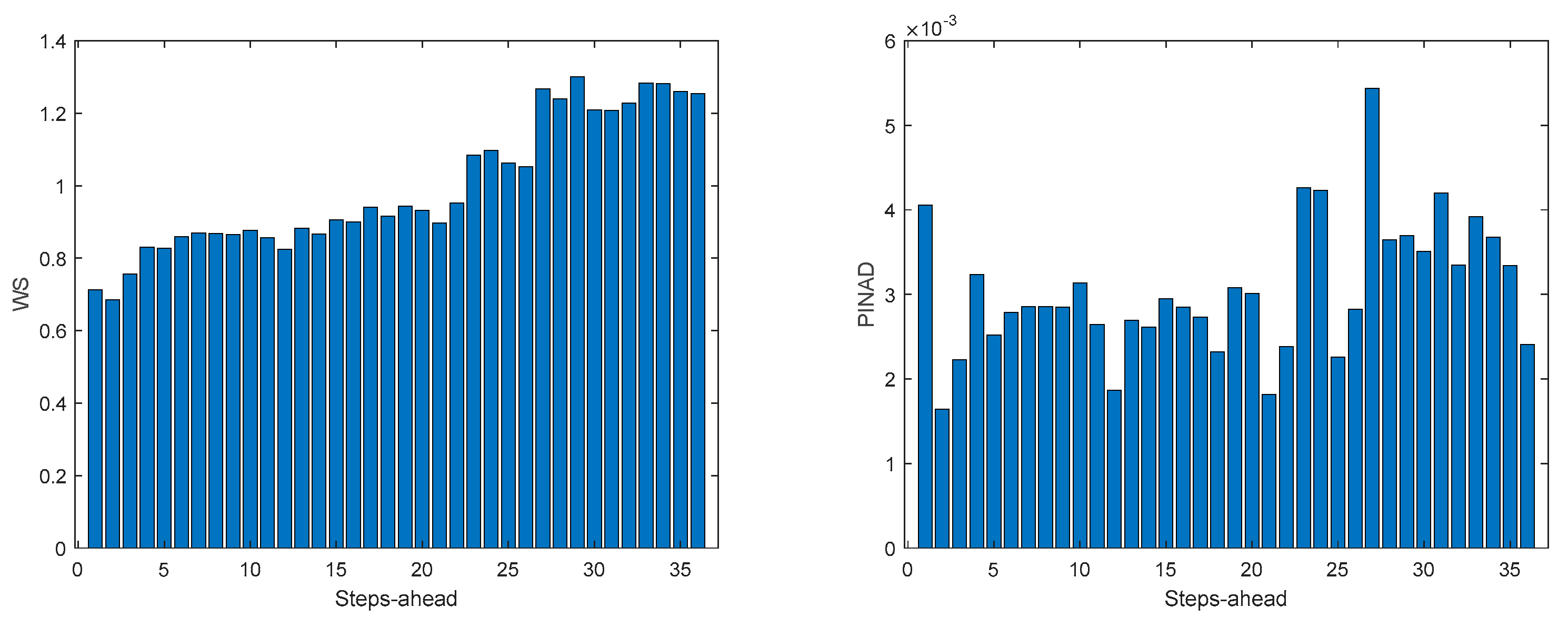
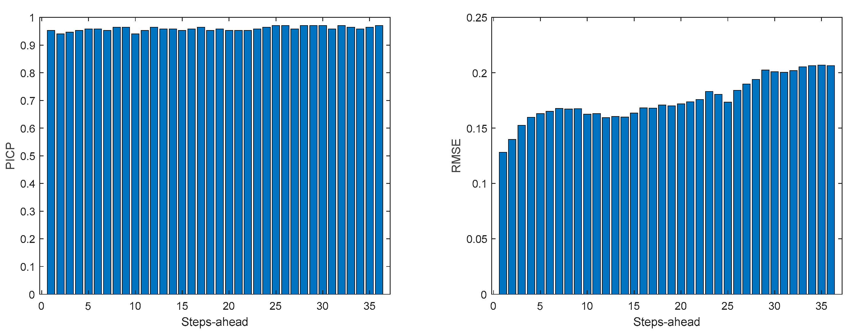
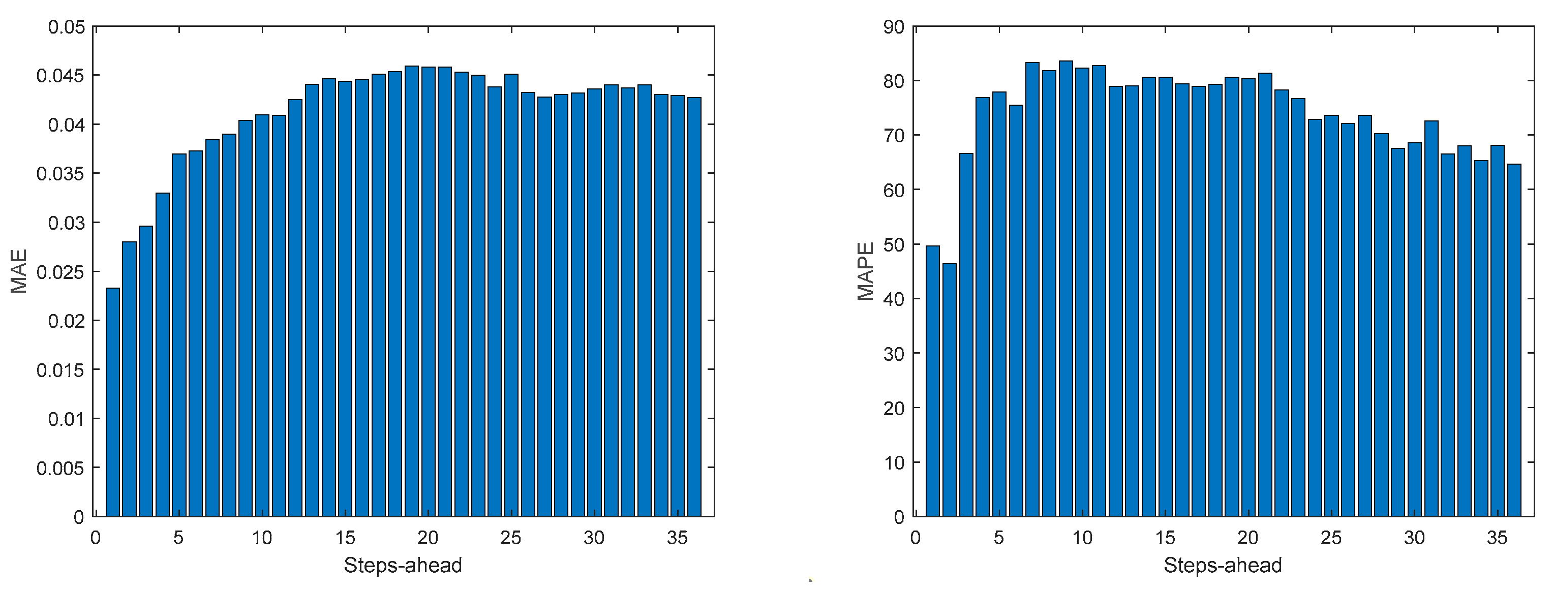
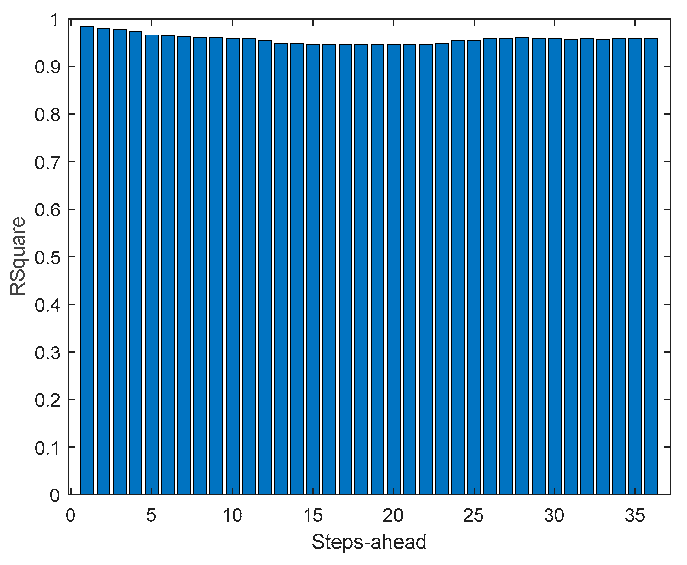
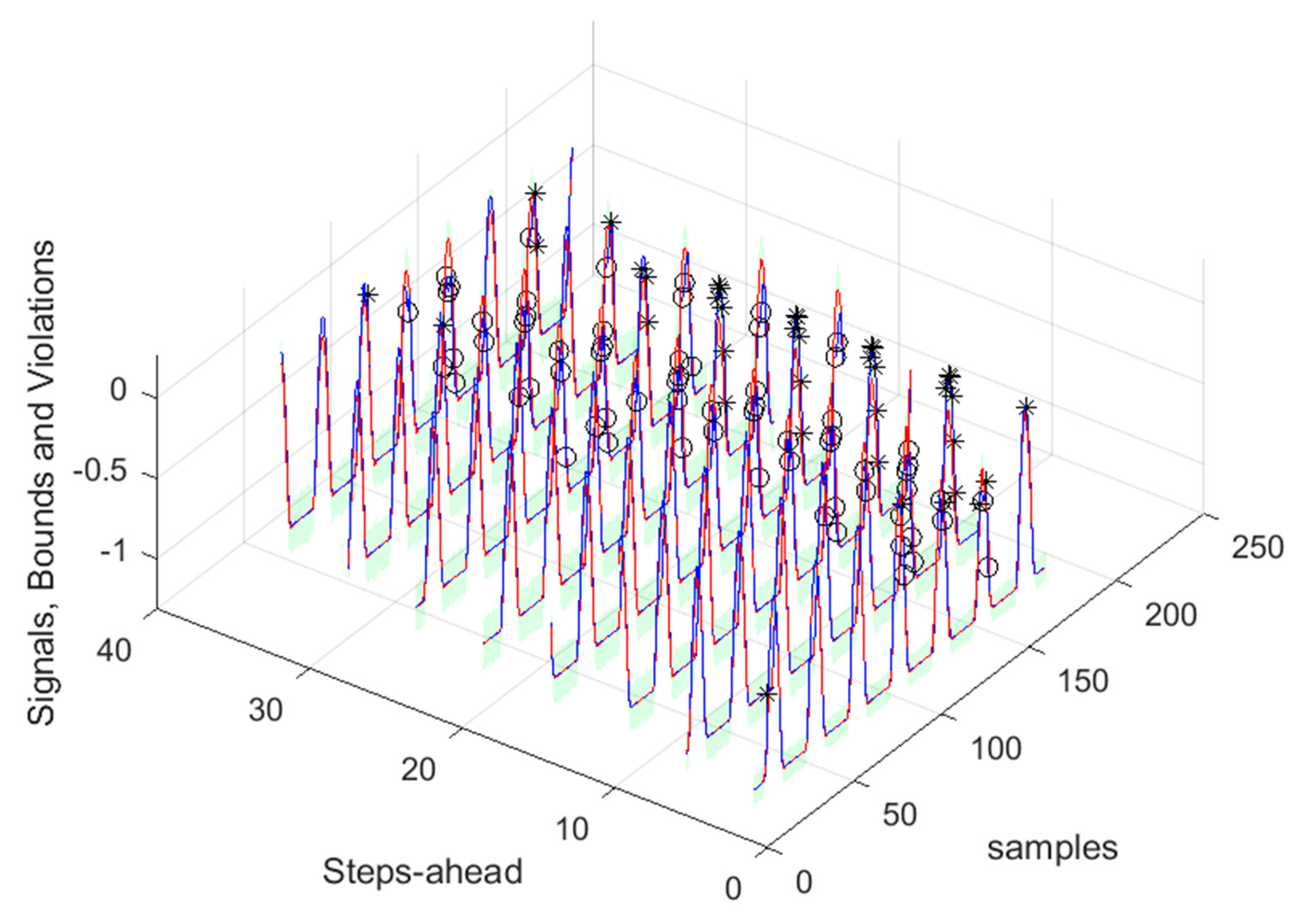
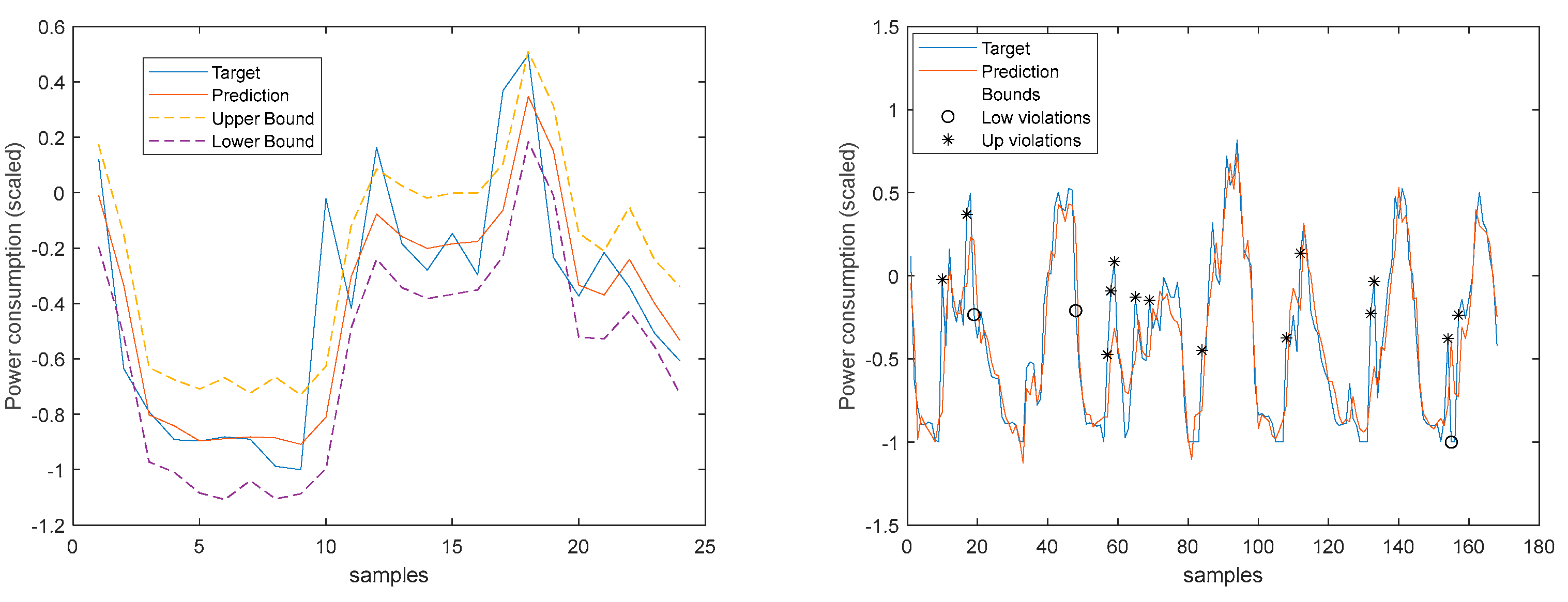
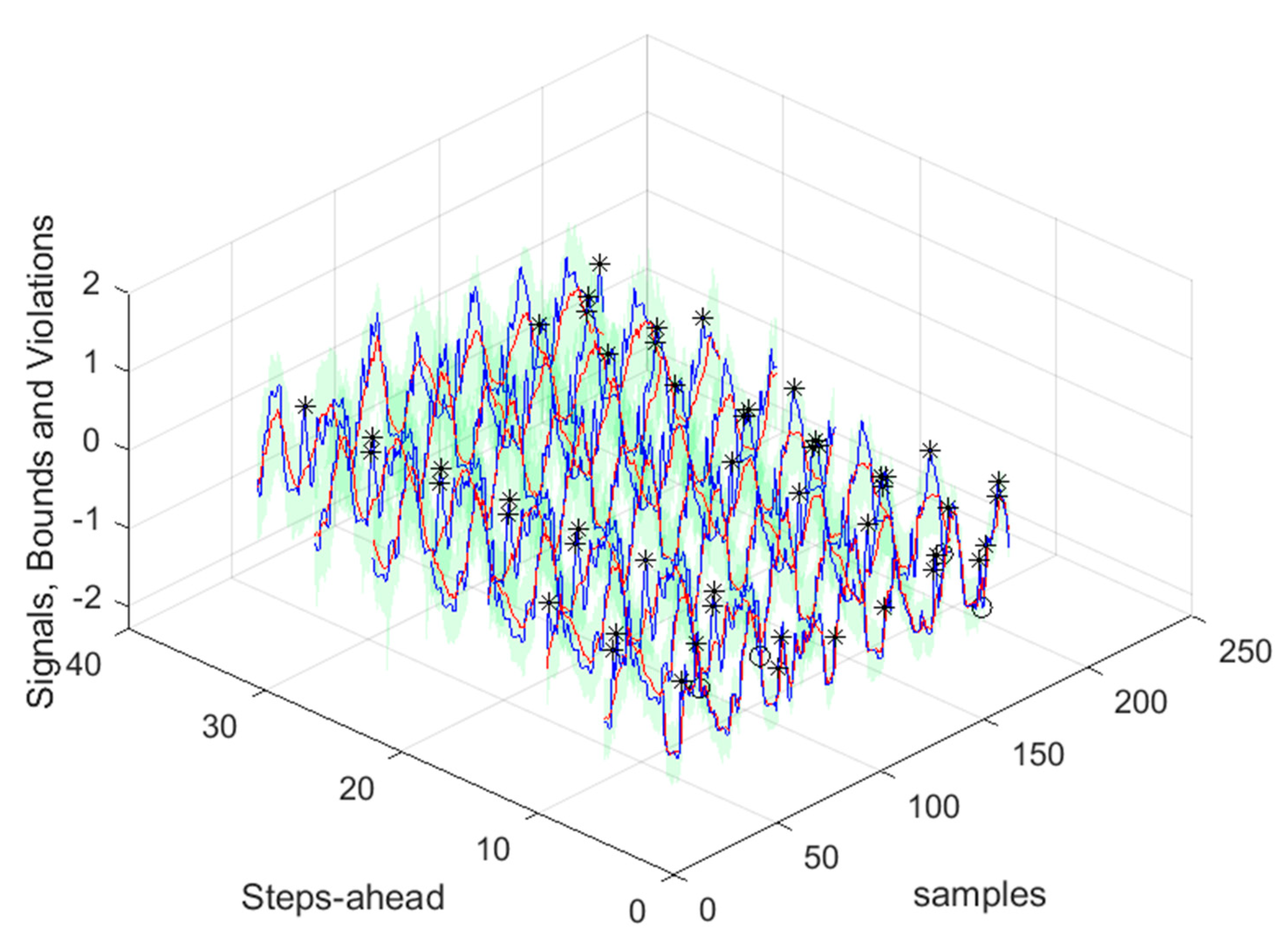
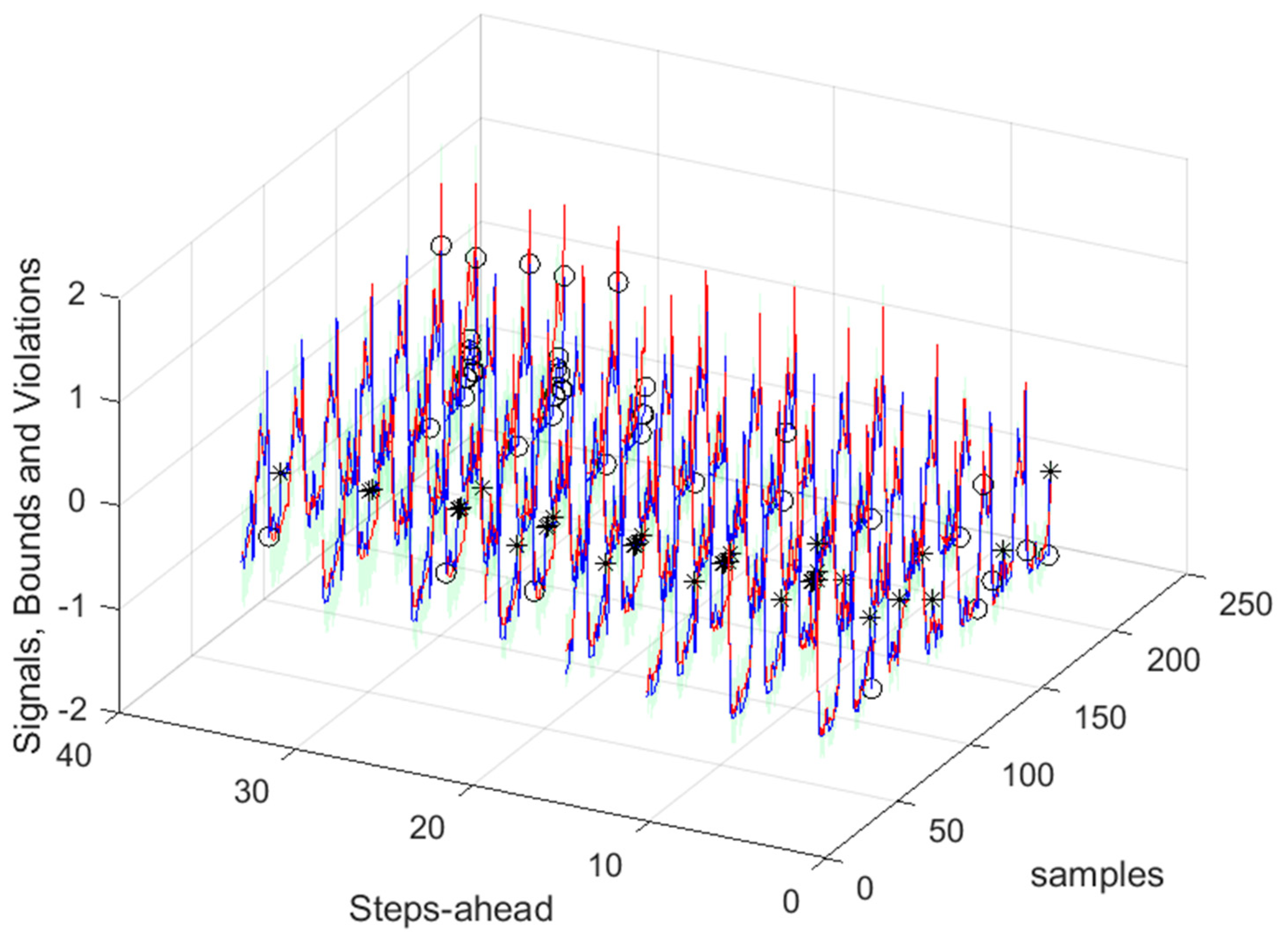
As it can be concluded analyzing
Table 2 and
Figure 10,
Figure 11,
Figure 12,
Figure 13,
Figure 14,
Figure 15,
Figure 16 and
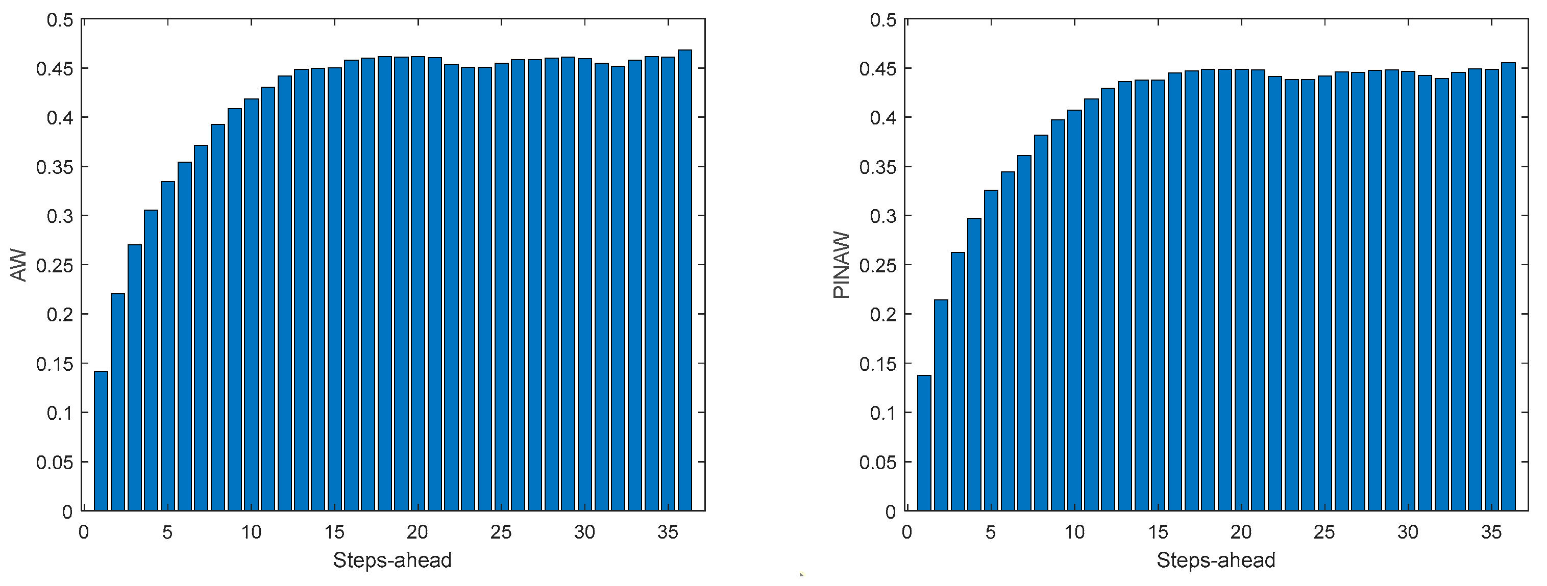
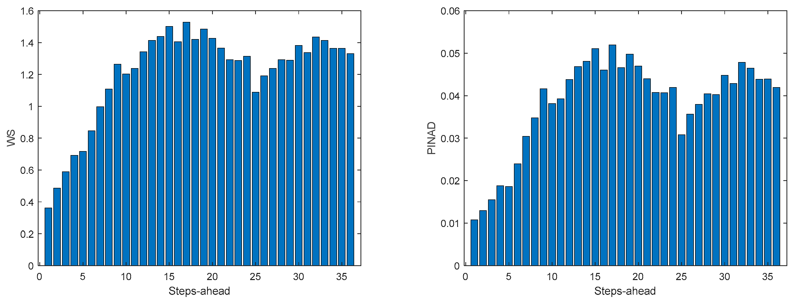
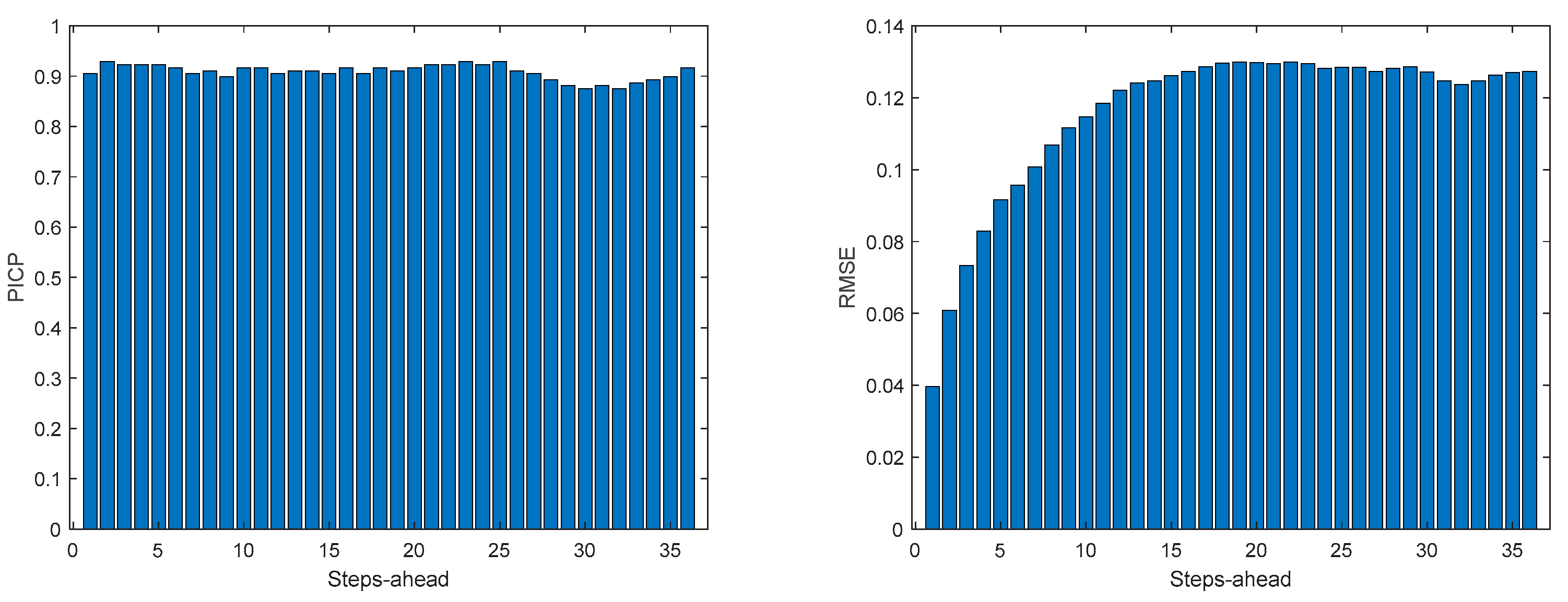
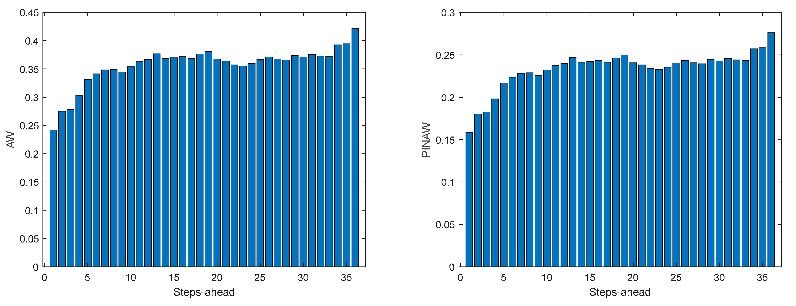
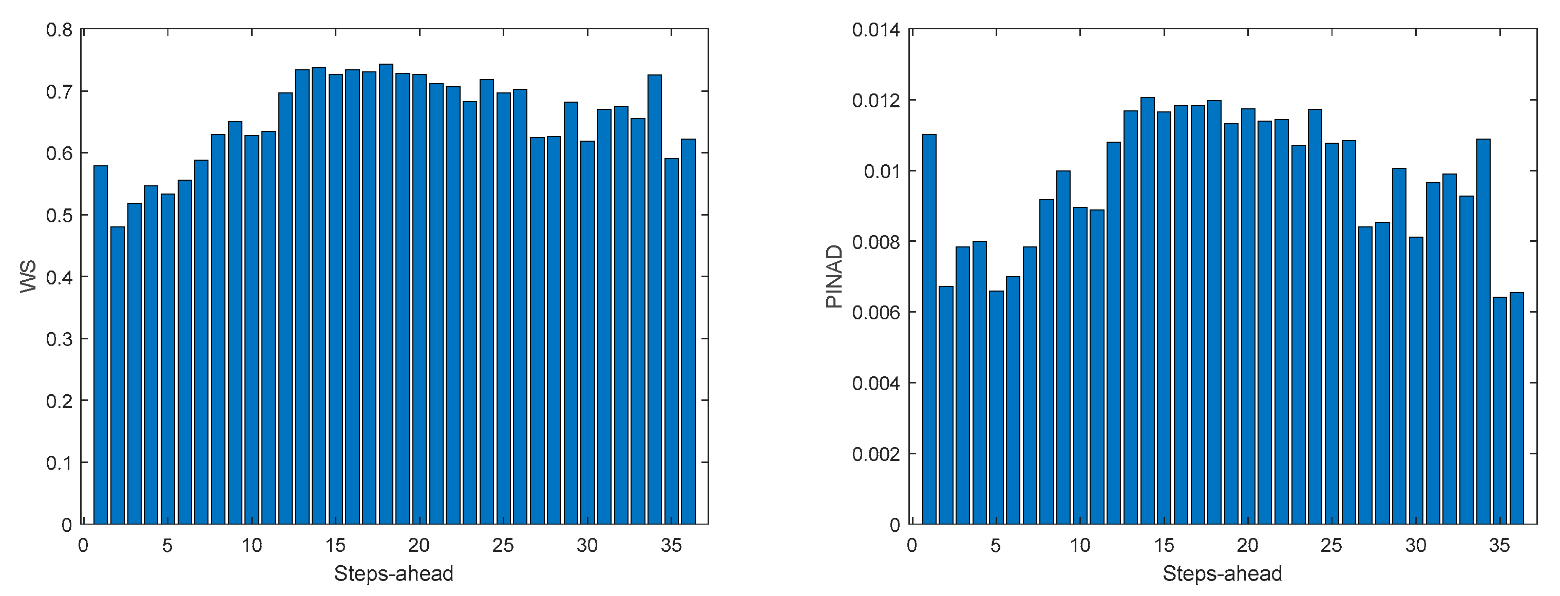
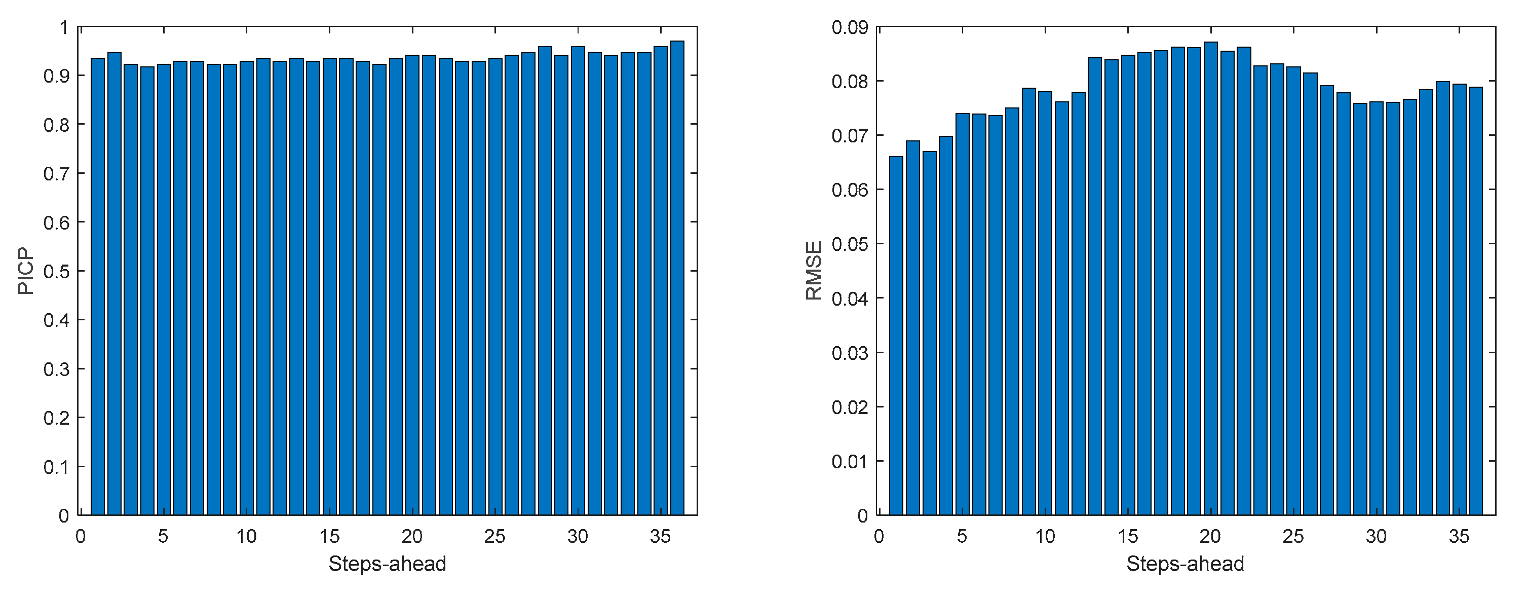
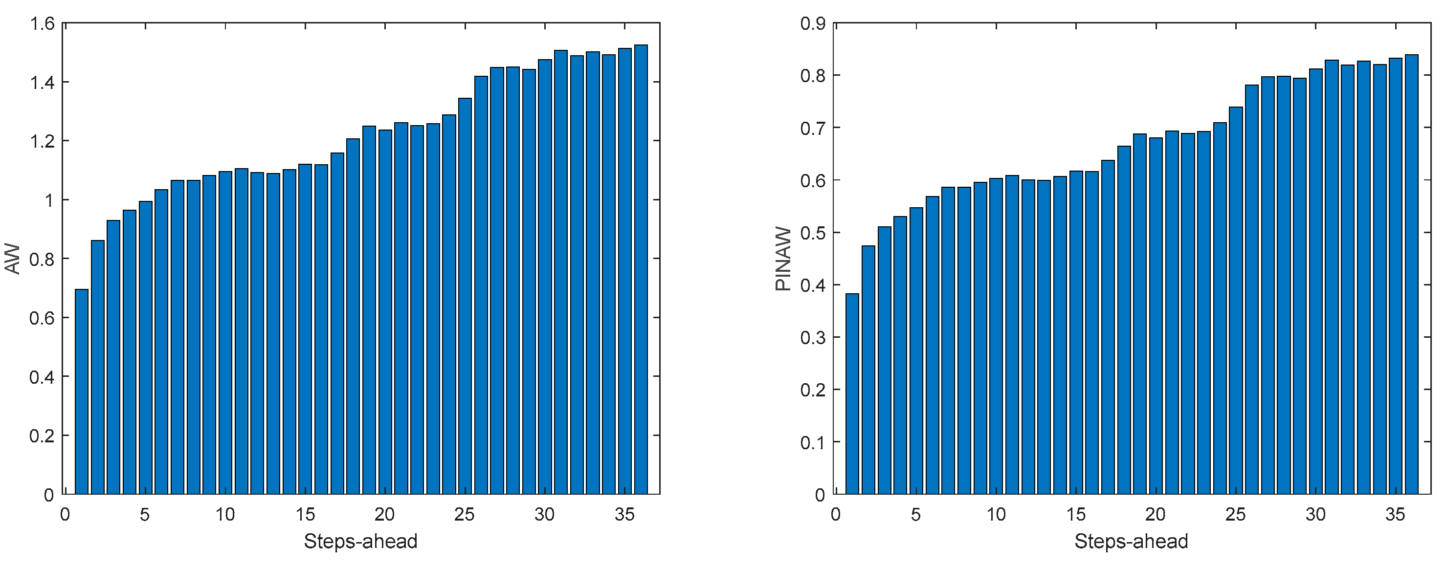
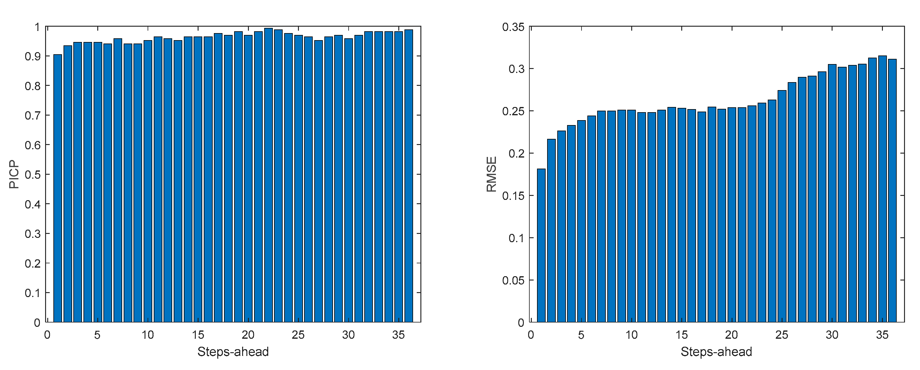
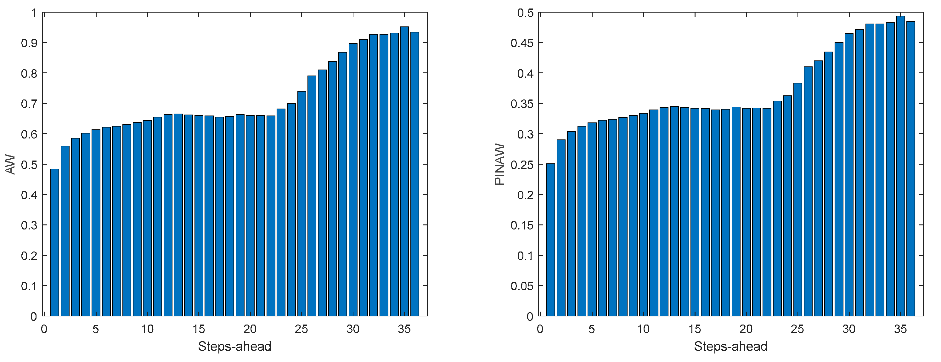
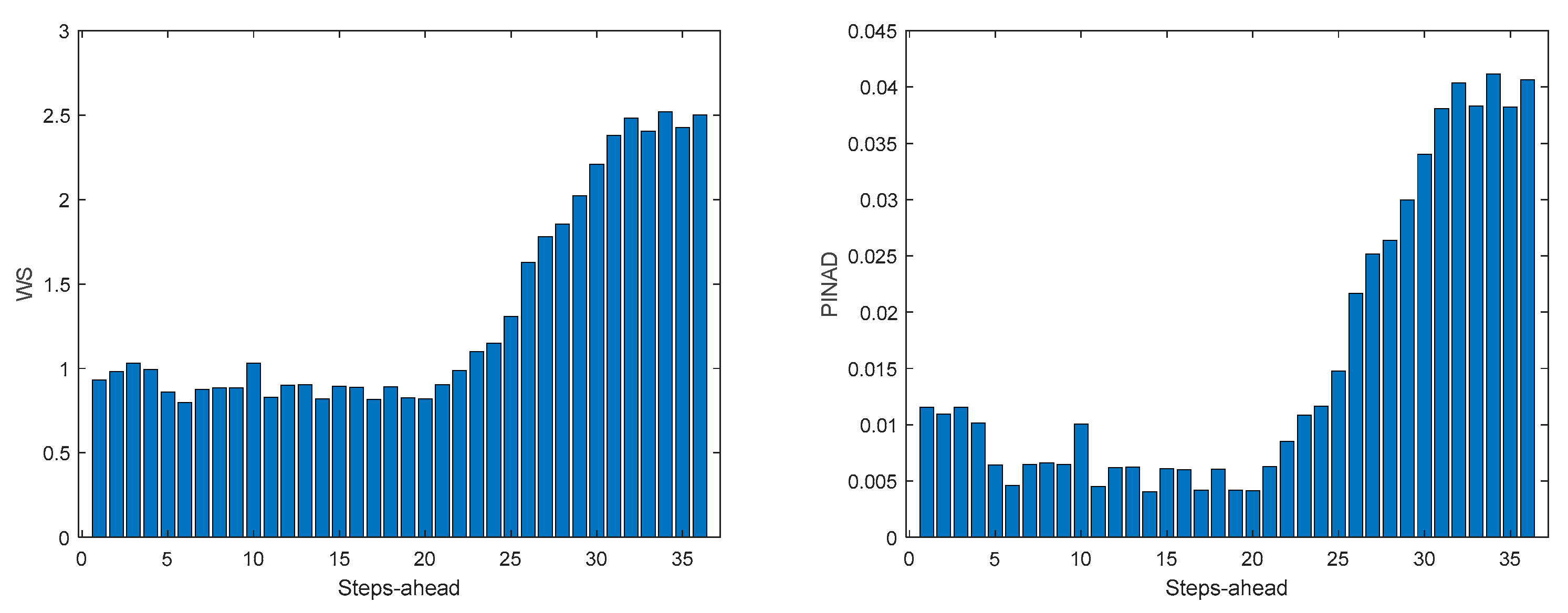
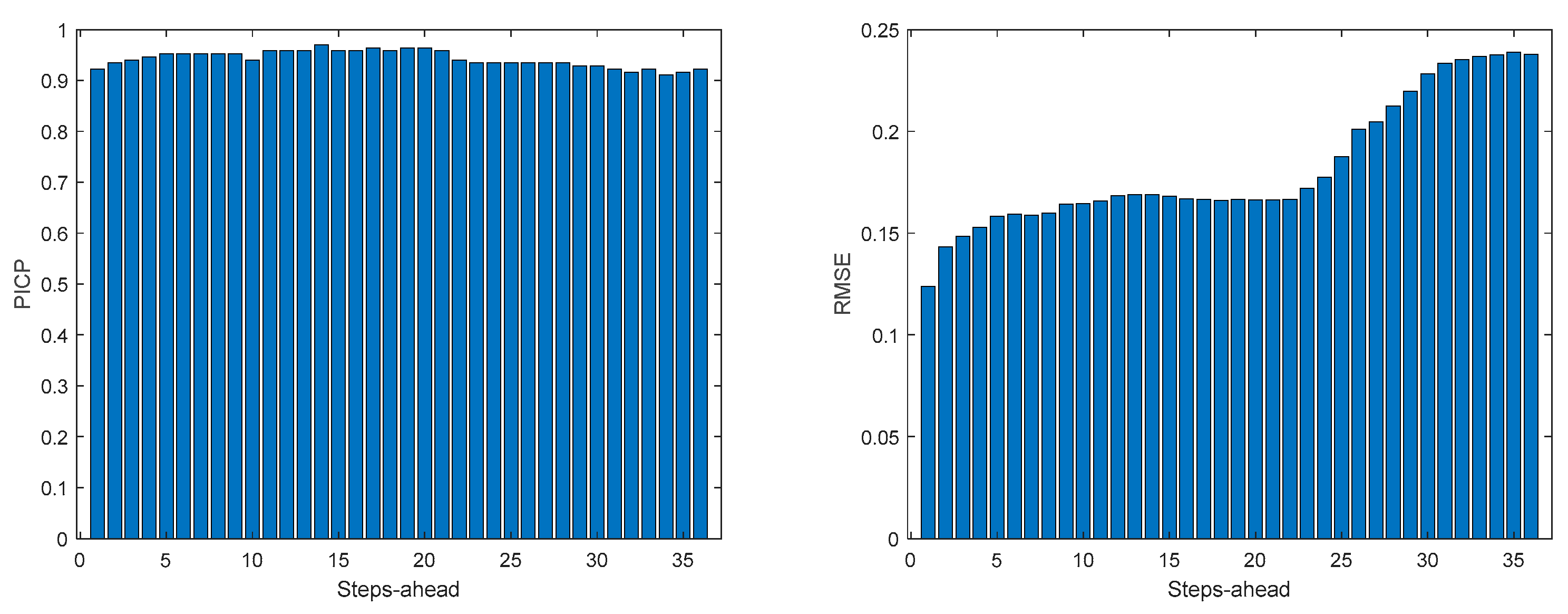
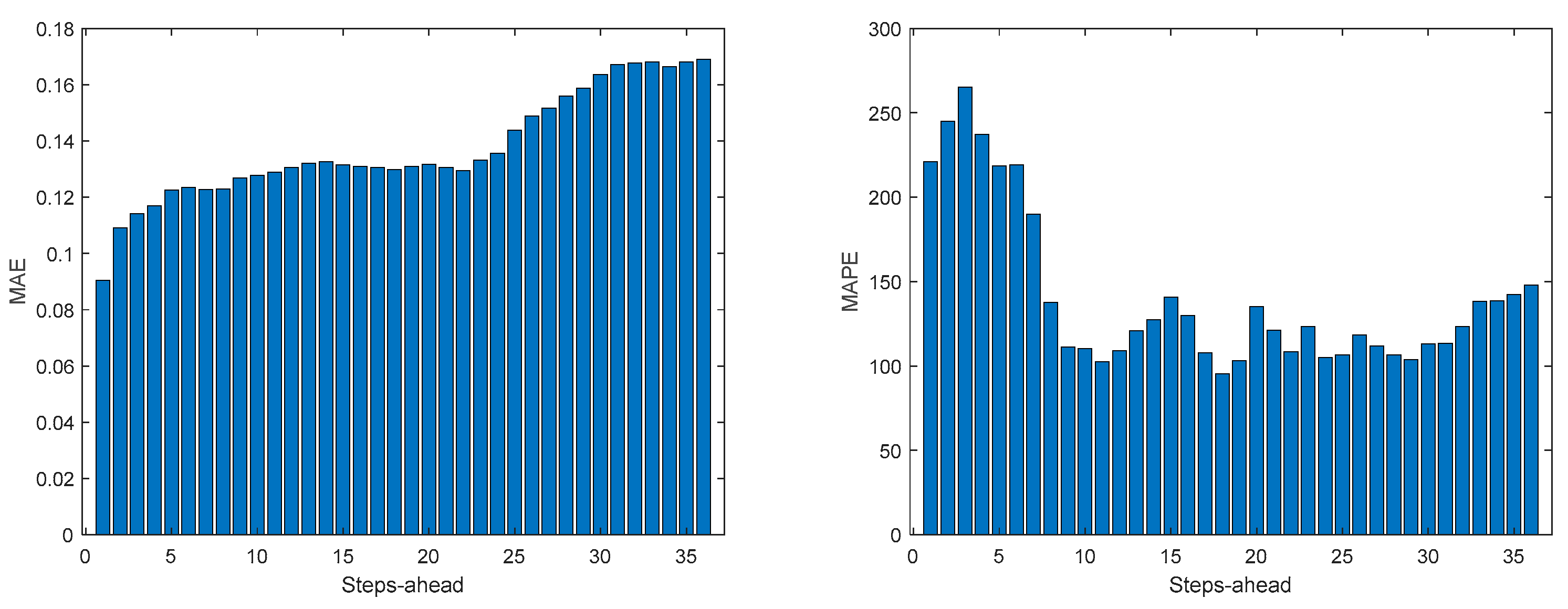
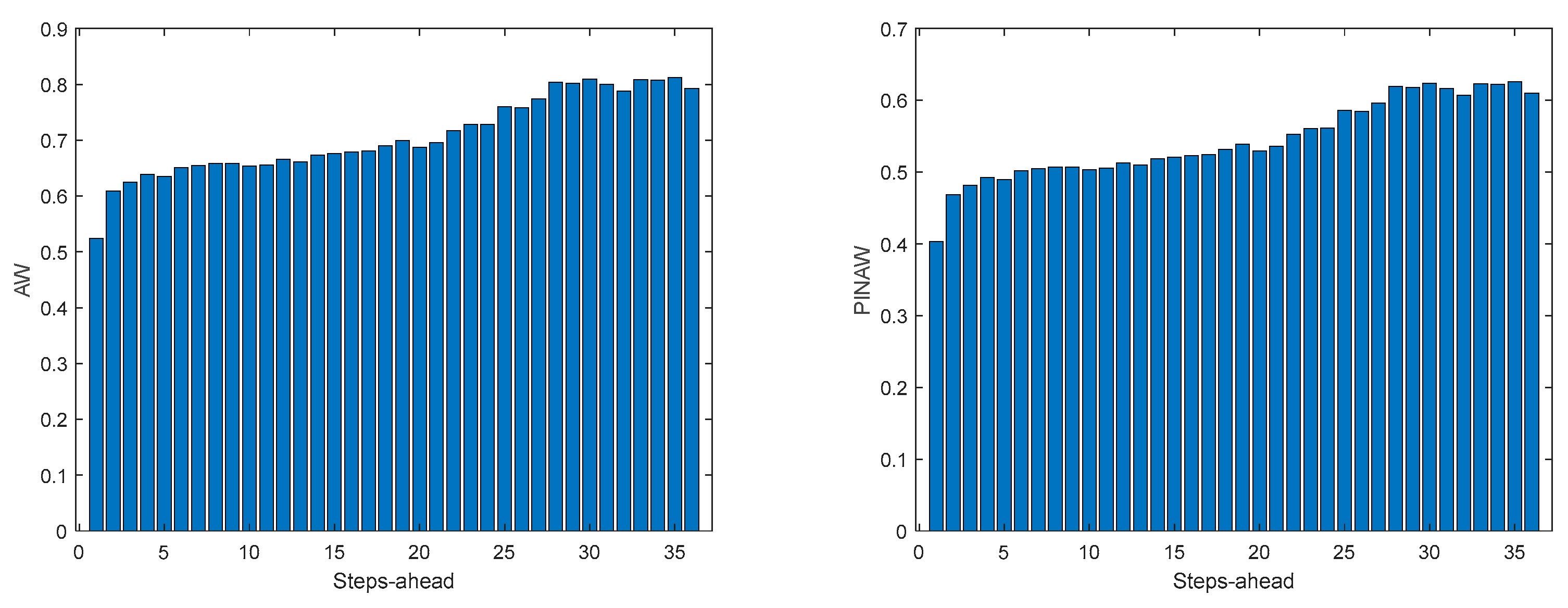
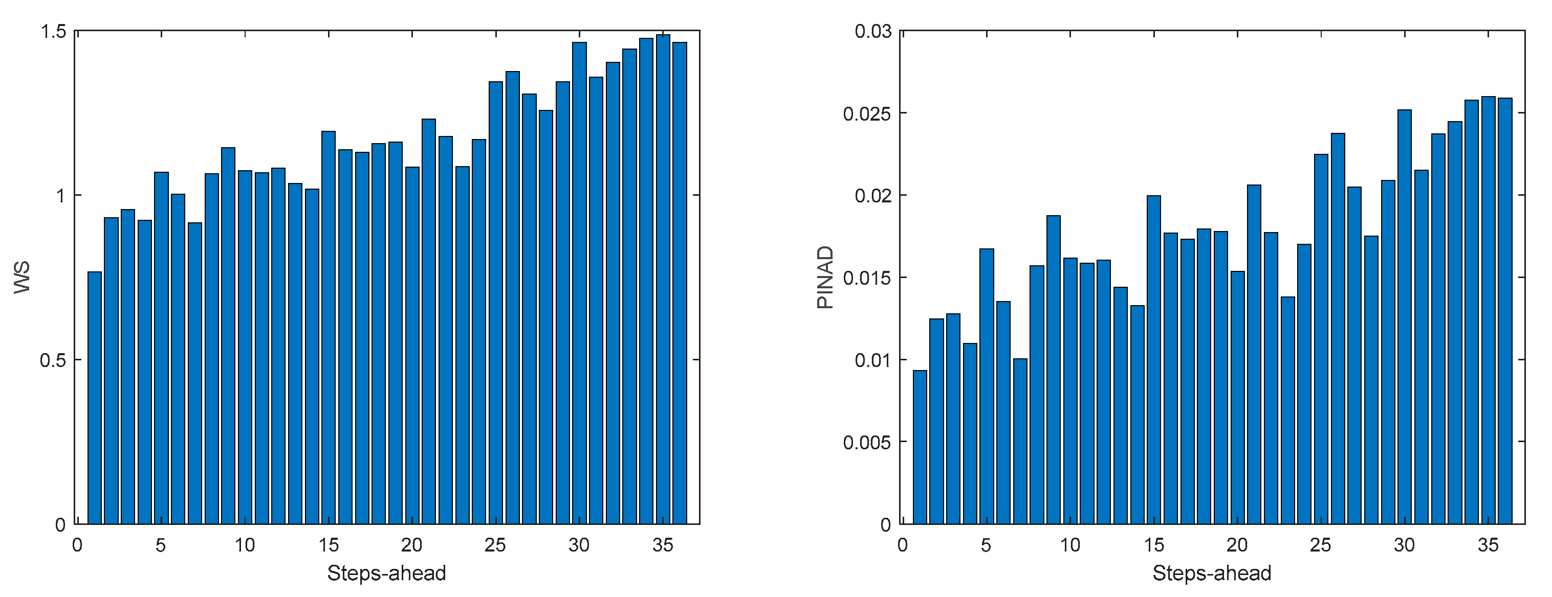
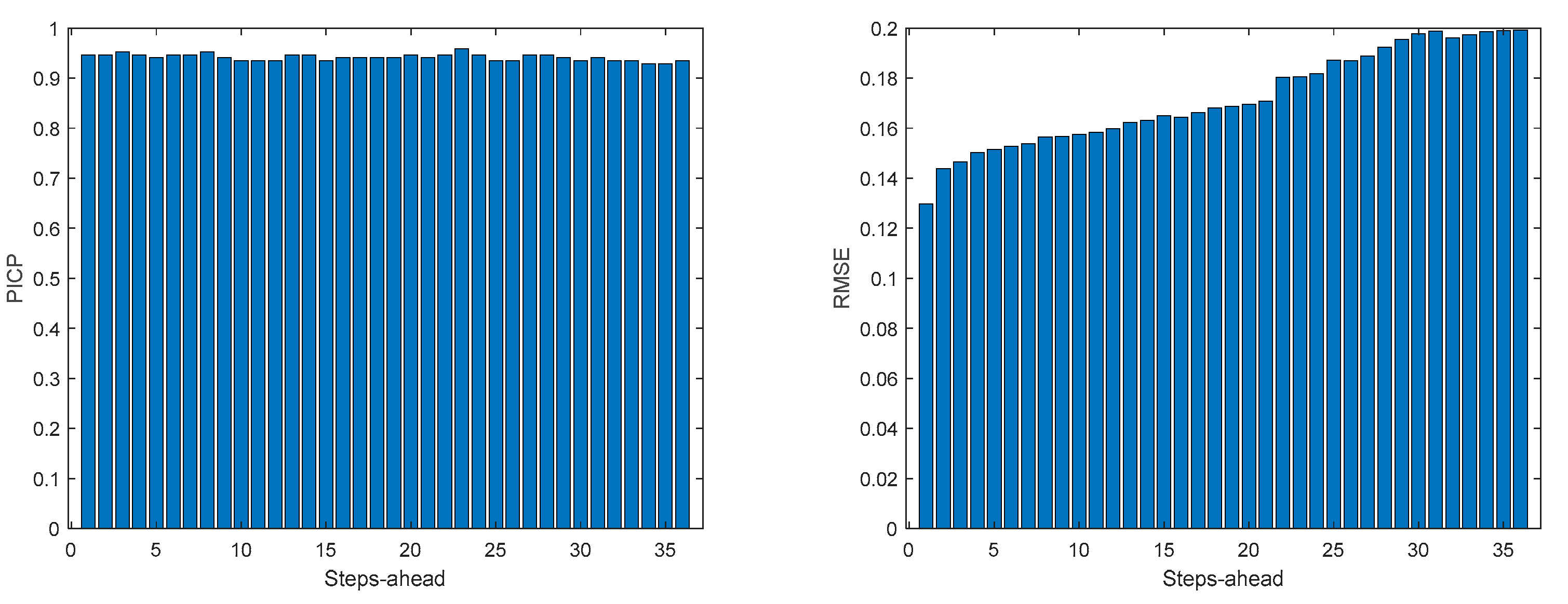
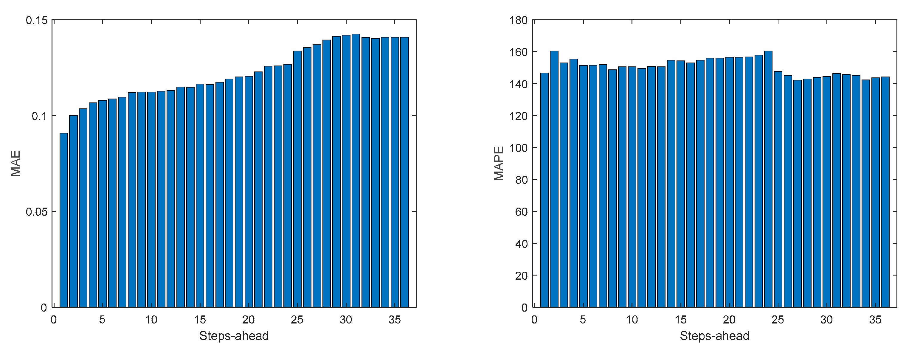
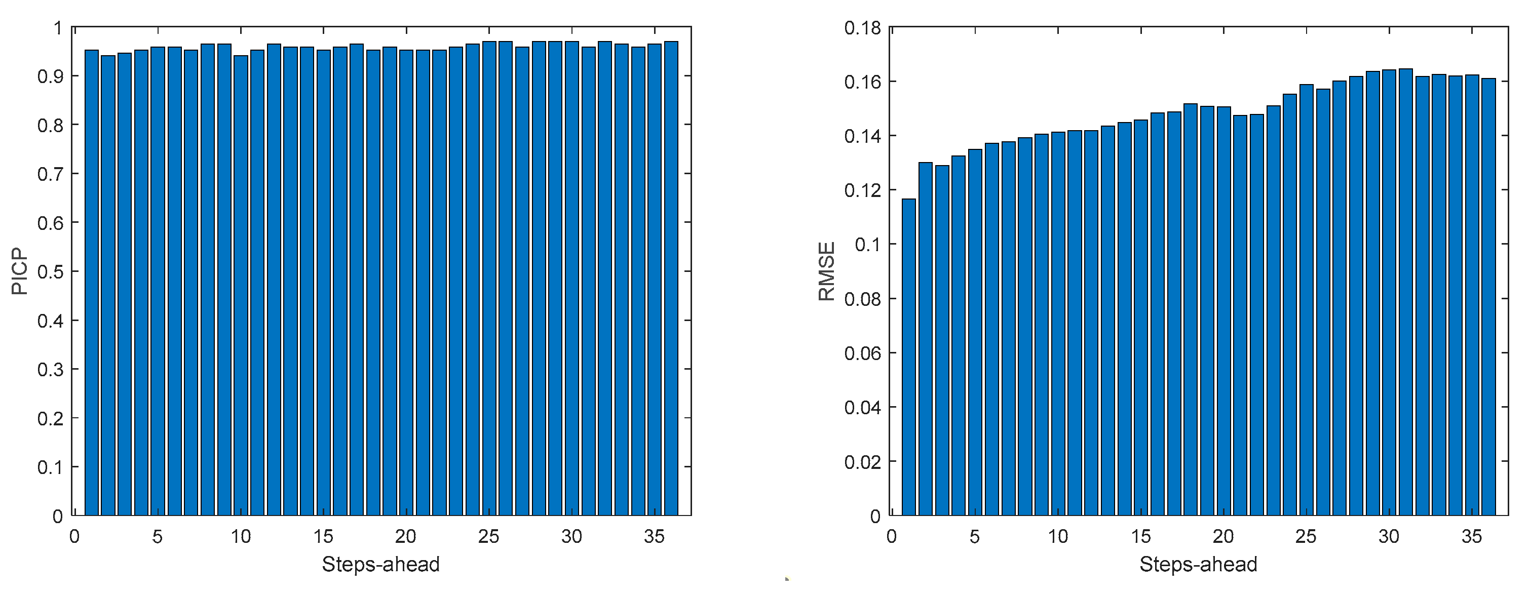
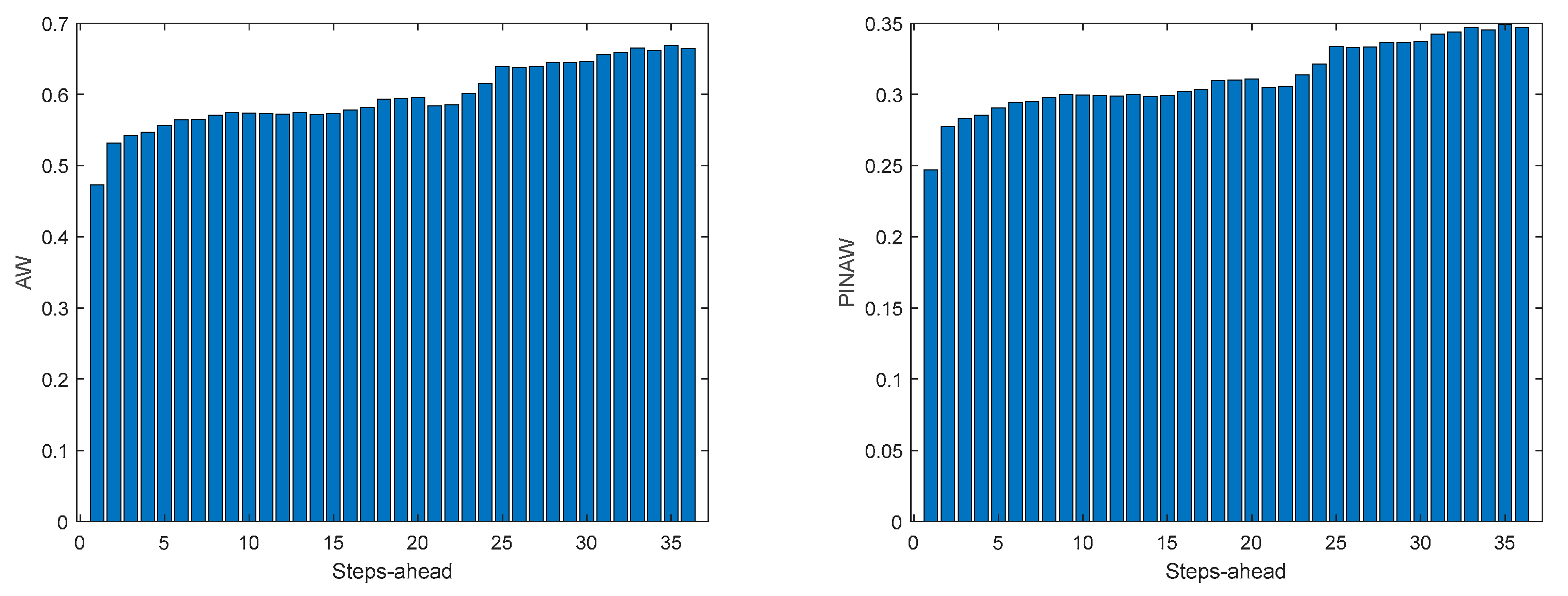
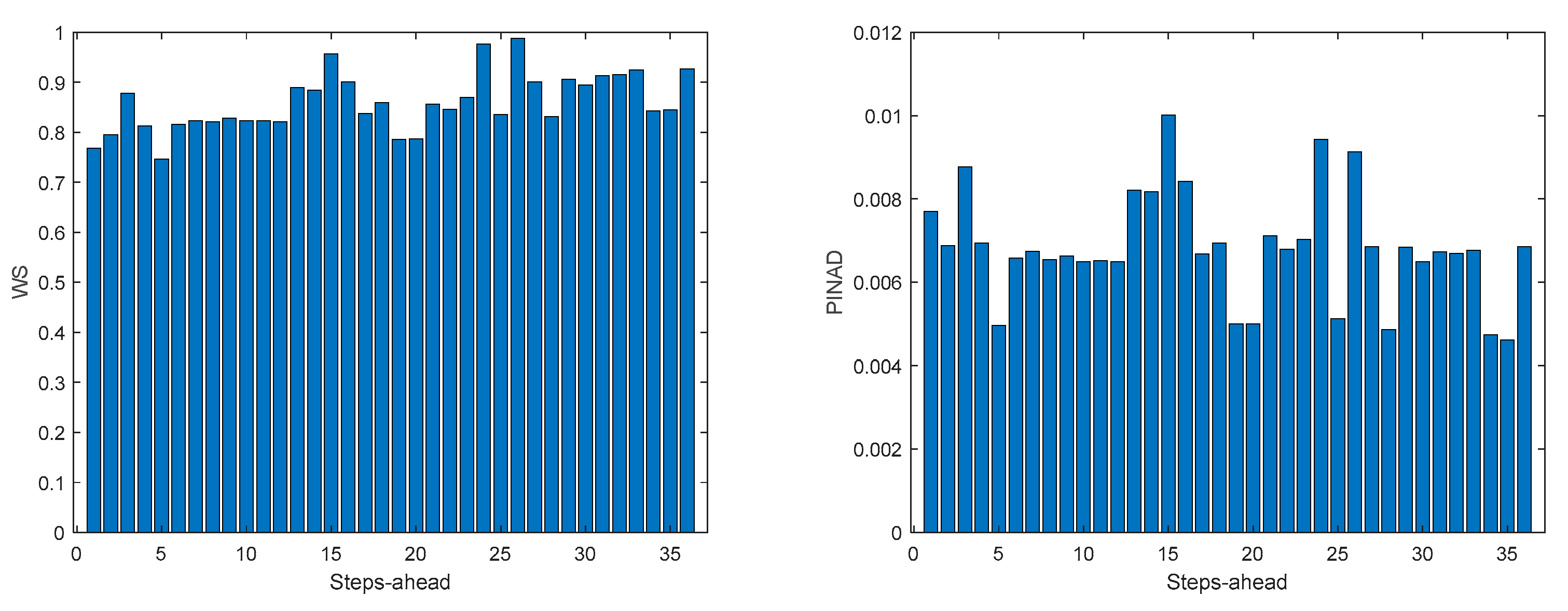
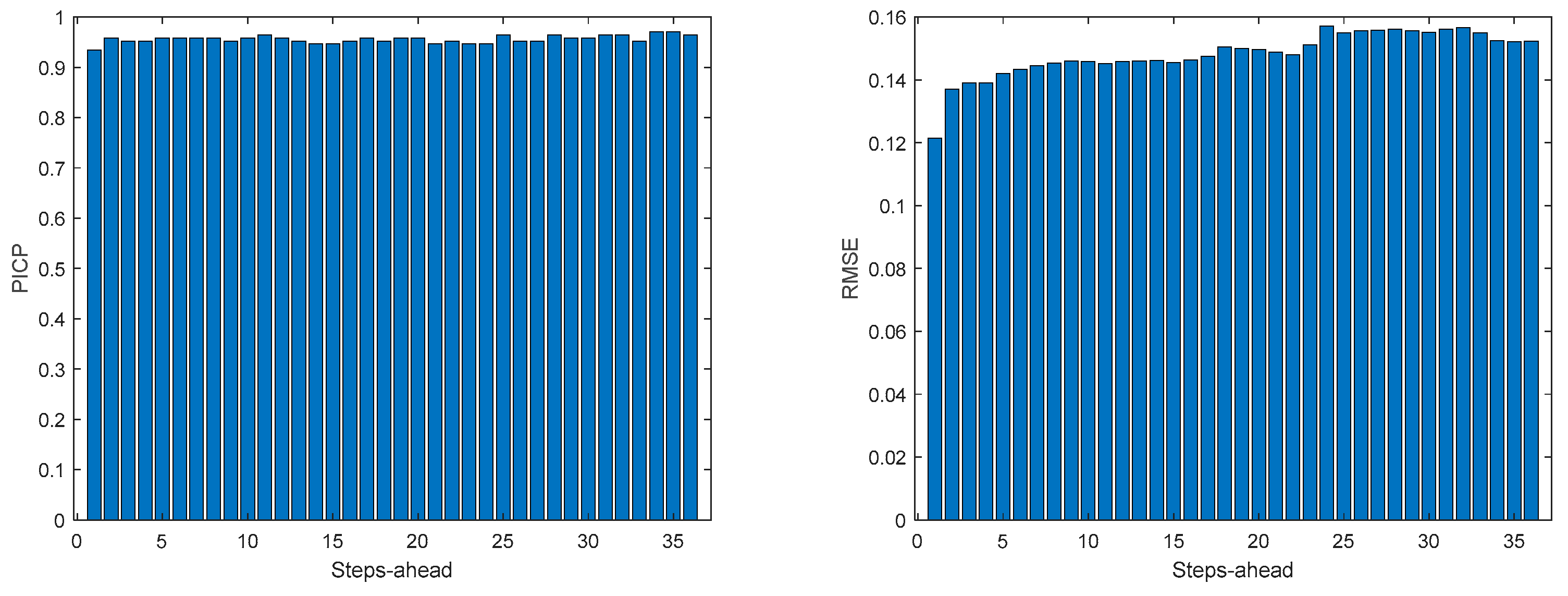
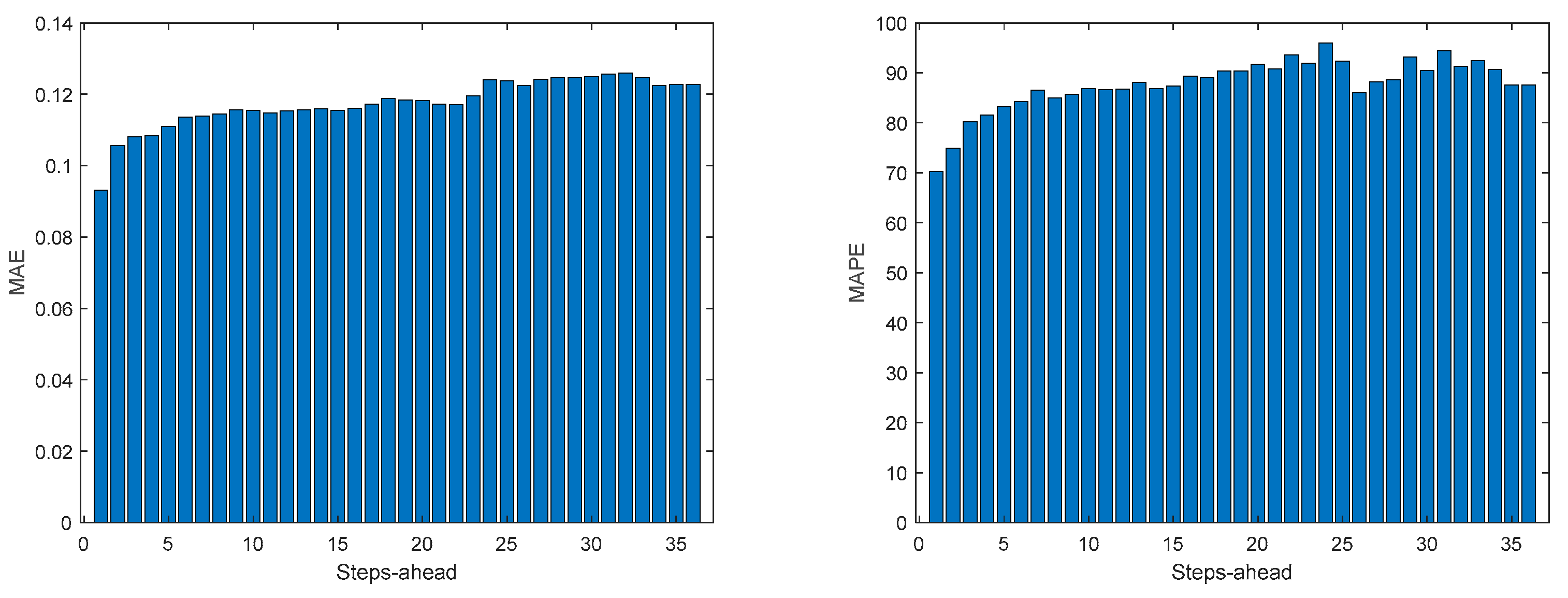
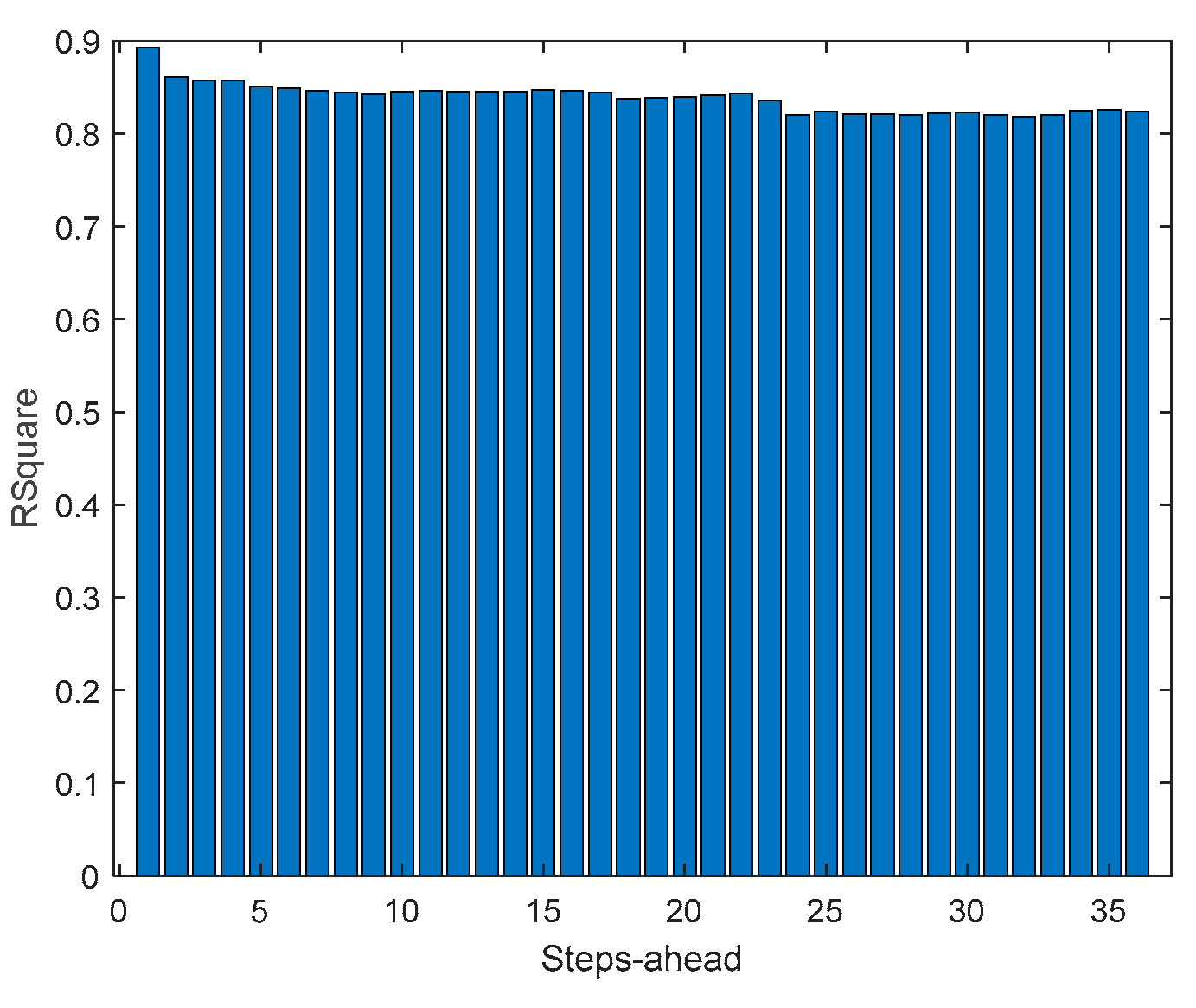
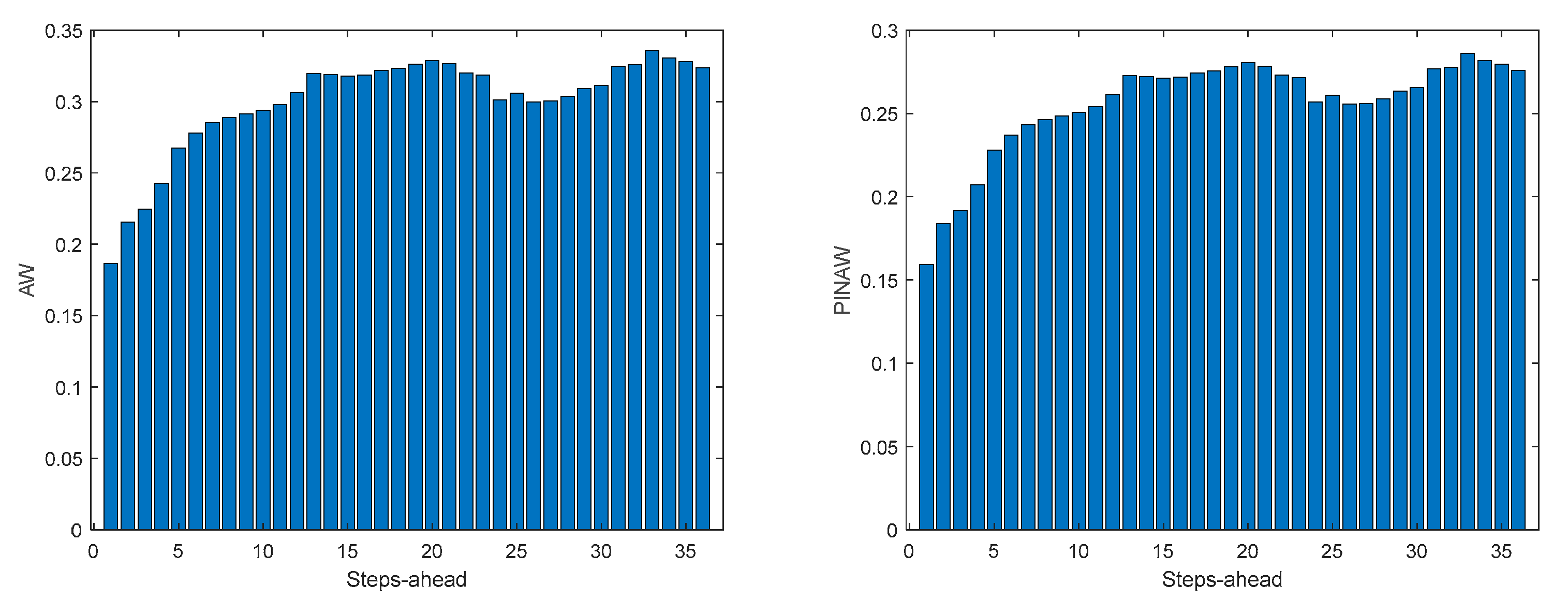
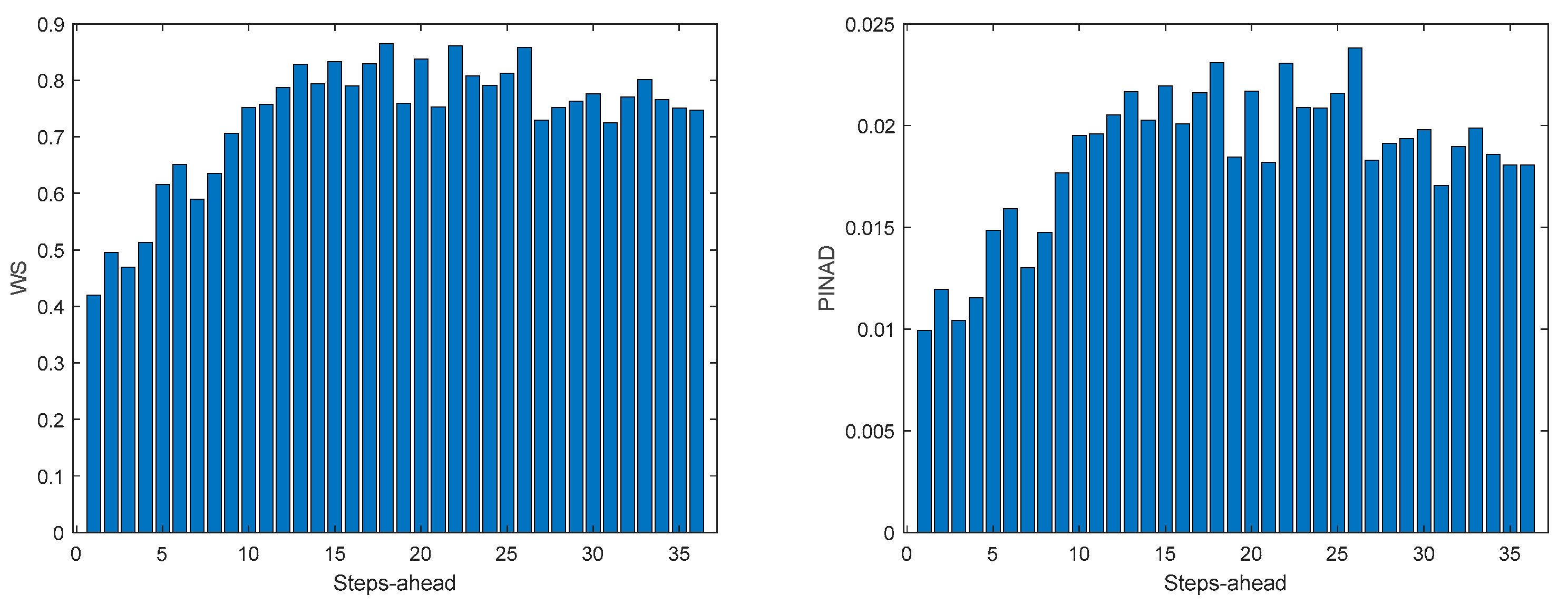
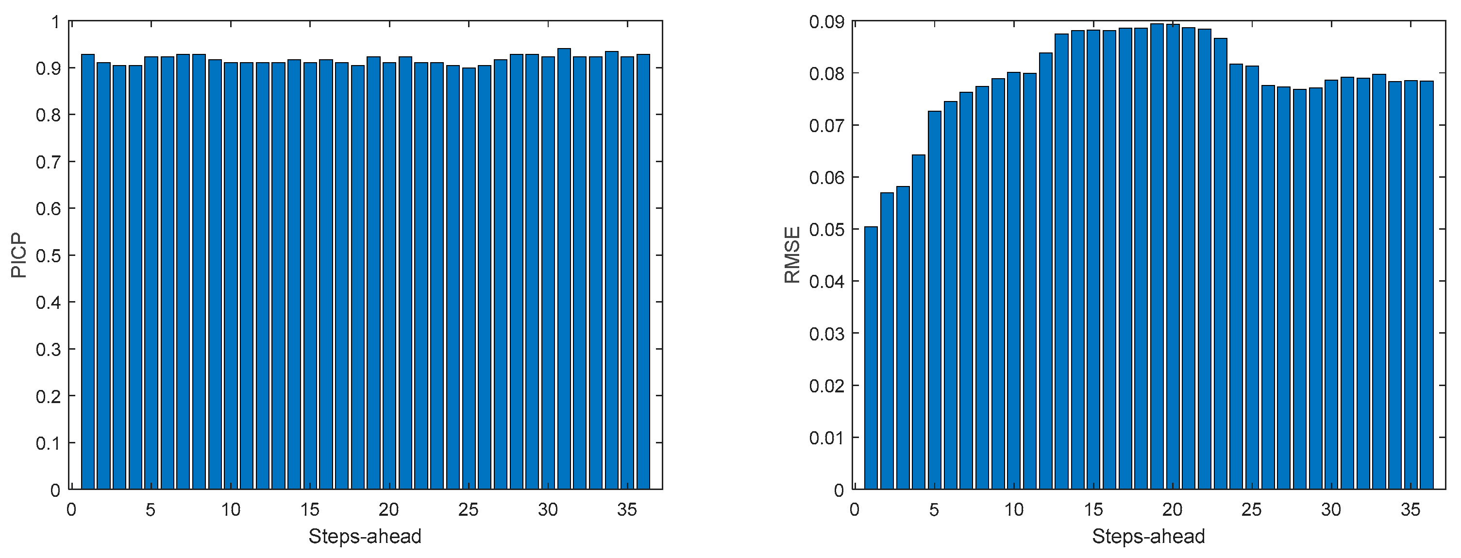
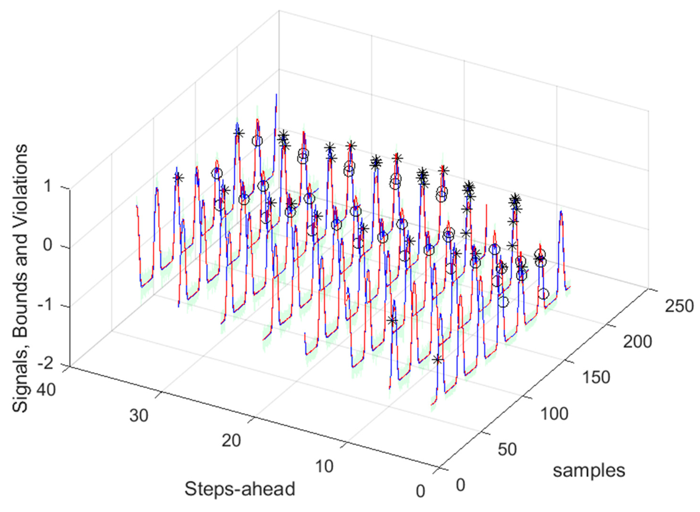
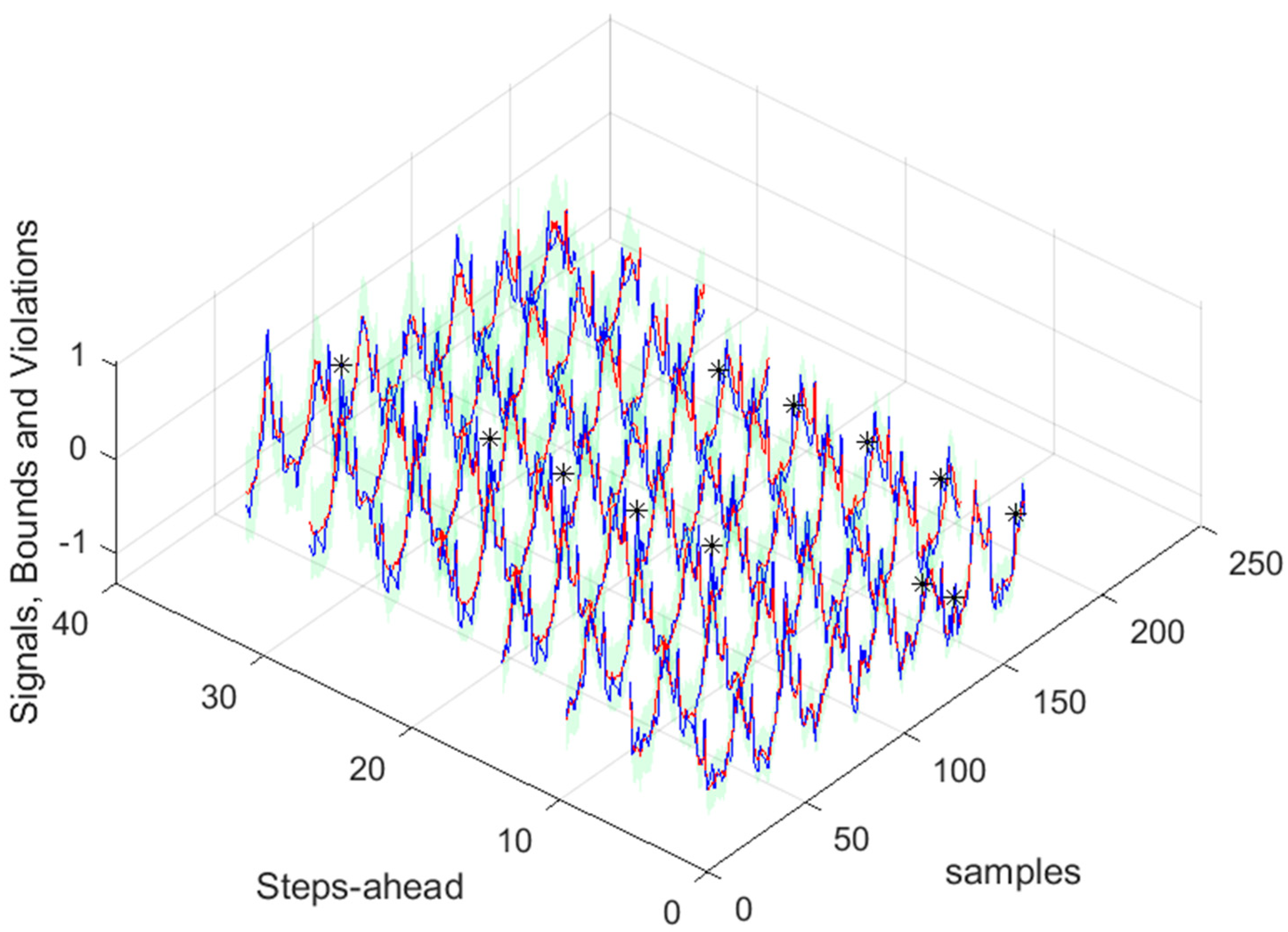
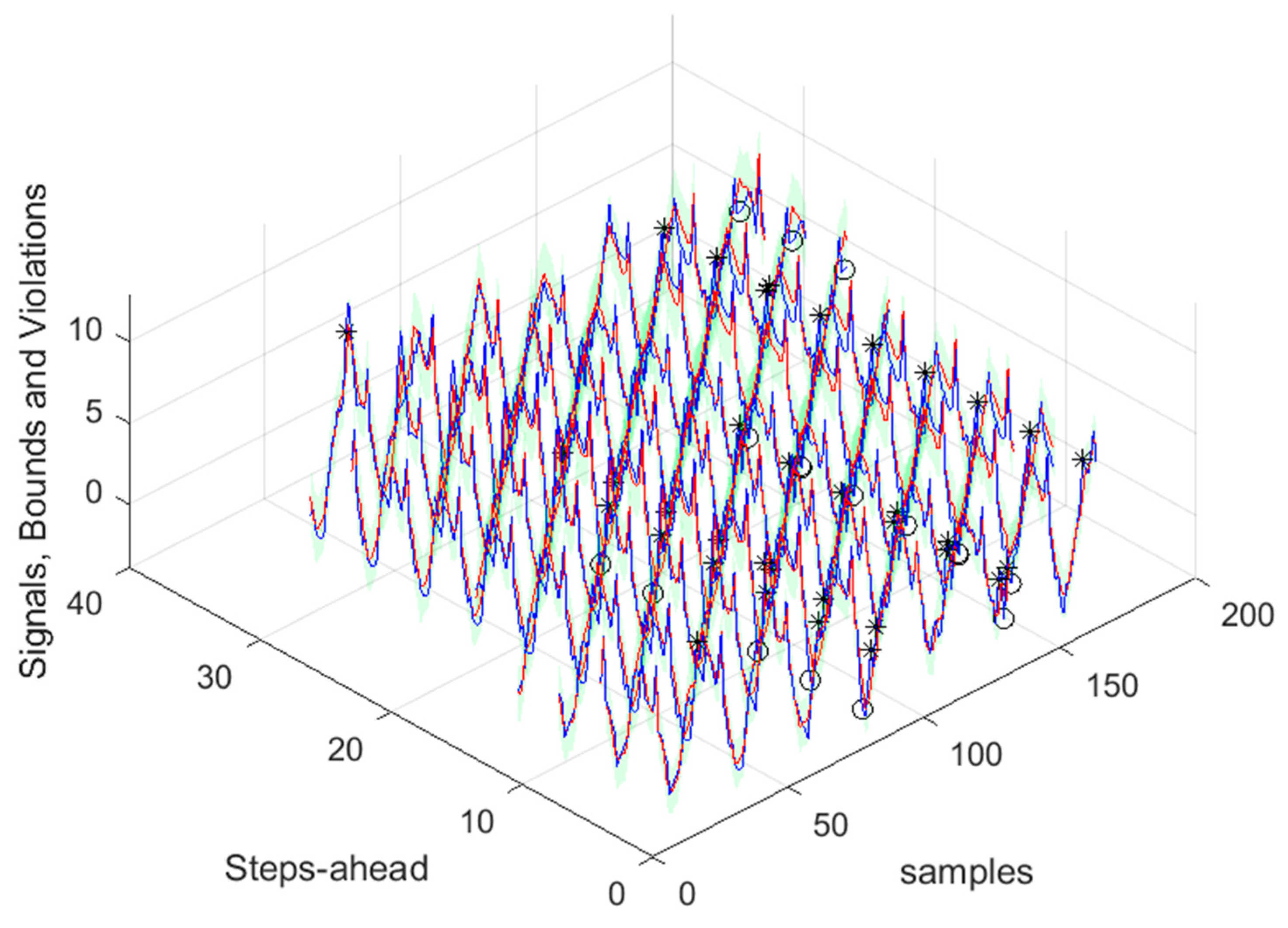
Figure 17, PICP does not vary significantly along PH, and is always greater than 0.9. The other robustness measures increase along the prediction horizon, but not significantly. Comparing AW and PINAW, they are related by a scale factor, corresponding to the range of the forecasted solar radiation along PH, which remains nearly constant. Although the number of bound violations remains near constant over PH (please see PICP-
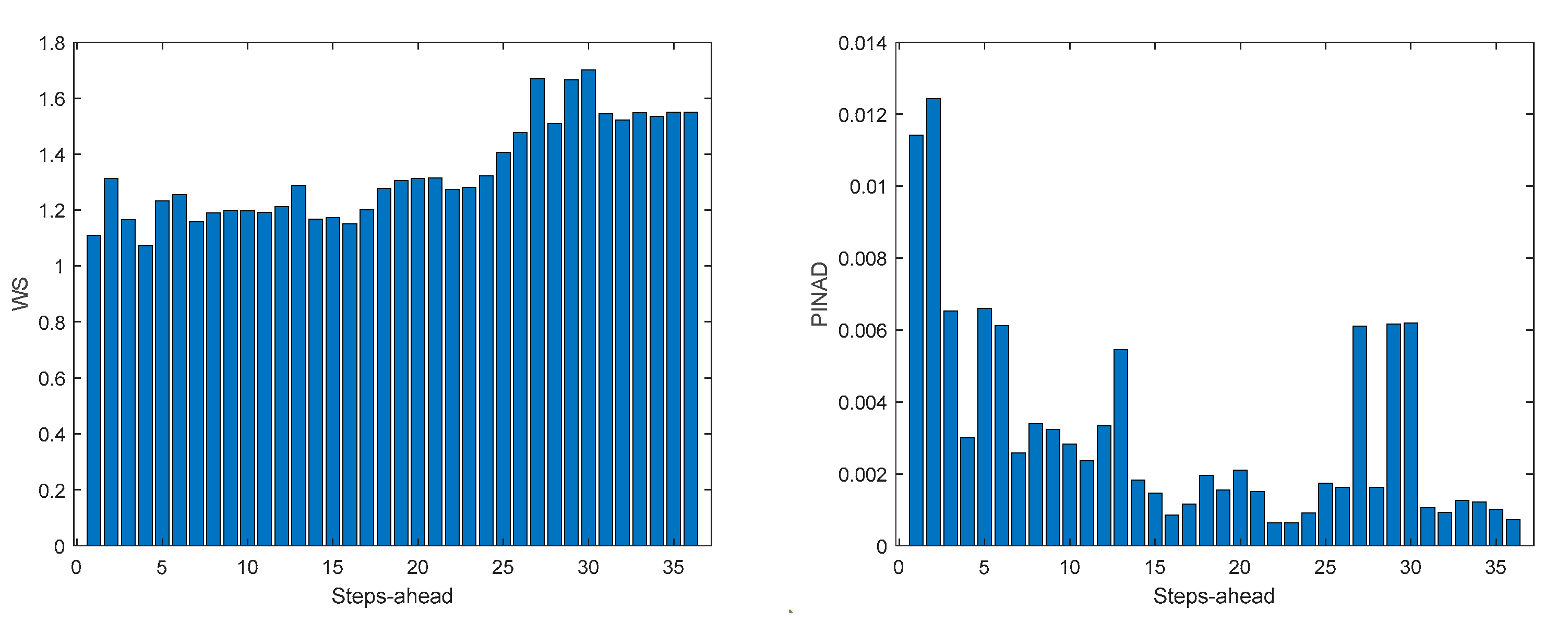
Figure 12 left), the range of the violations changes with the step-ahead. This can be confirmed by PINAD evolution (
Figure 11 right), and by the Winkler score evolution (
Figure 11 left), which penalizes twenty times the magnitude of the violations.
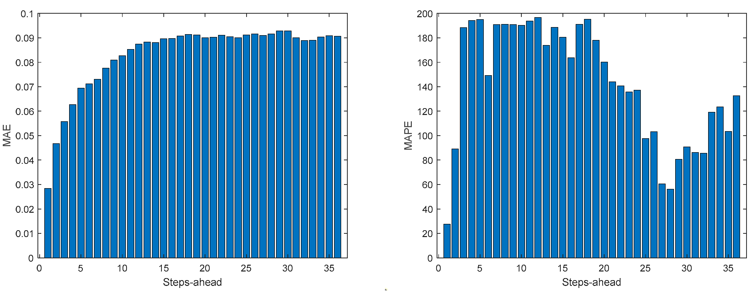
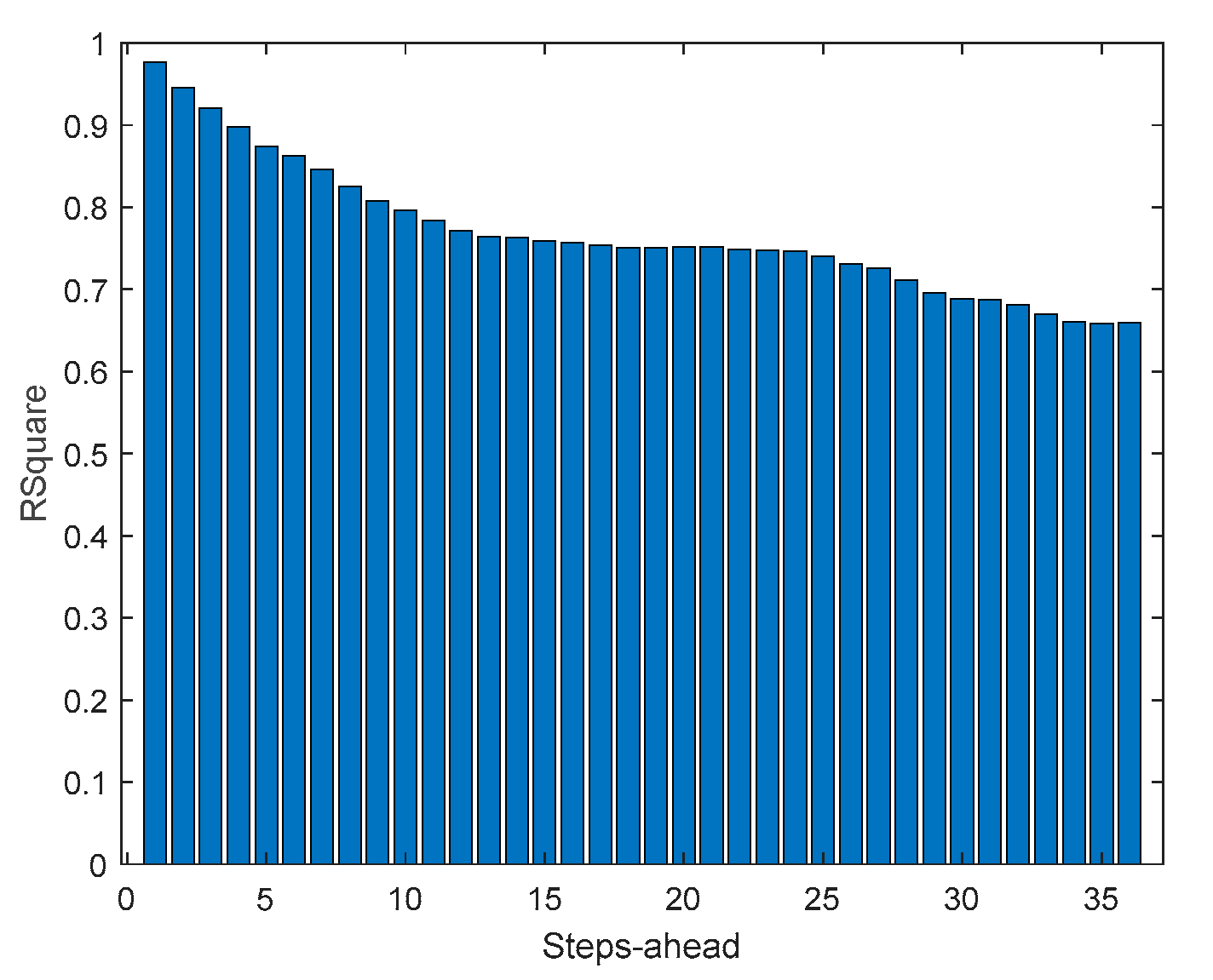
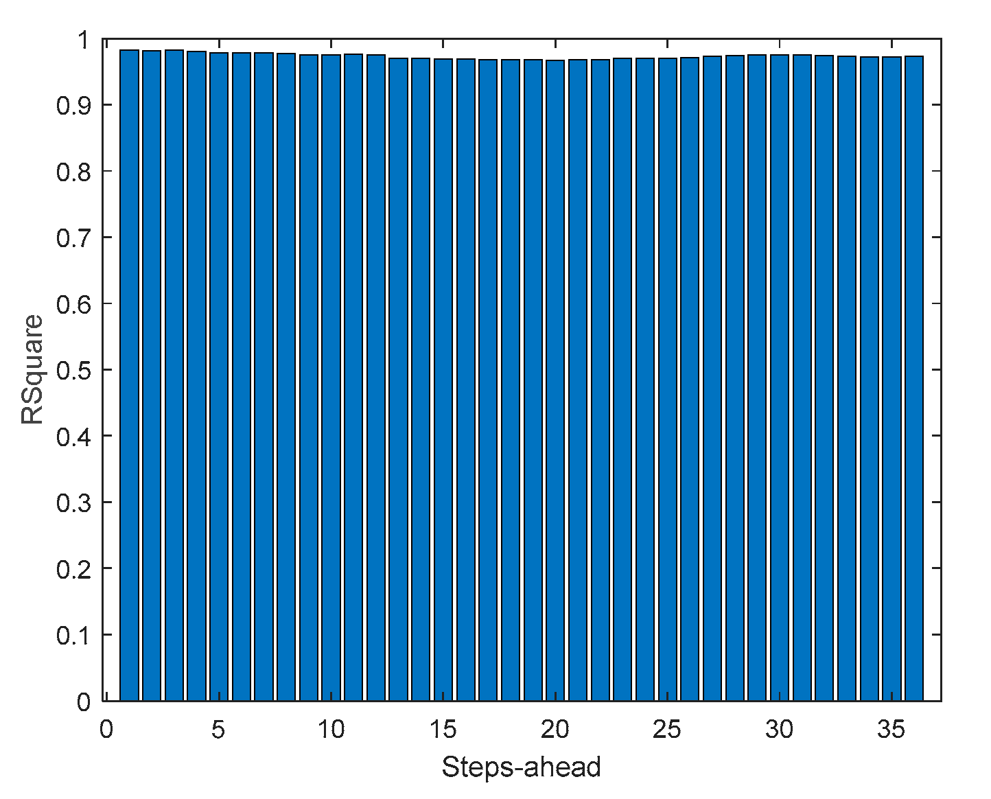
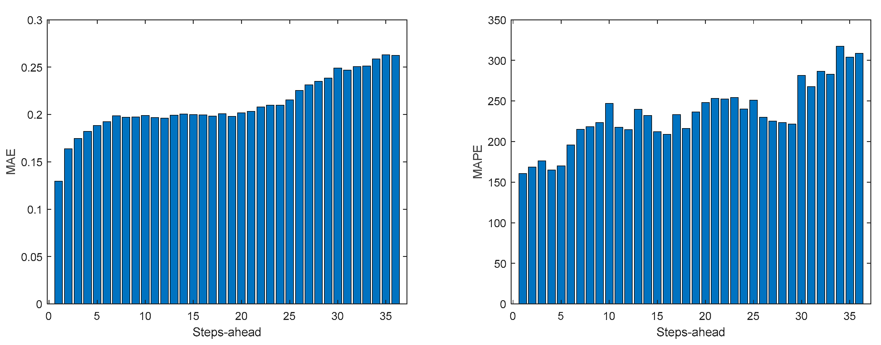
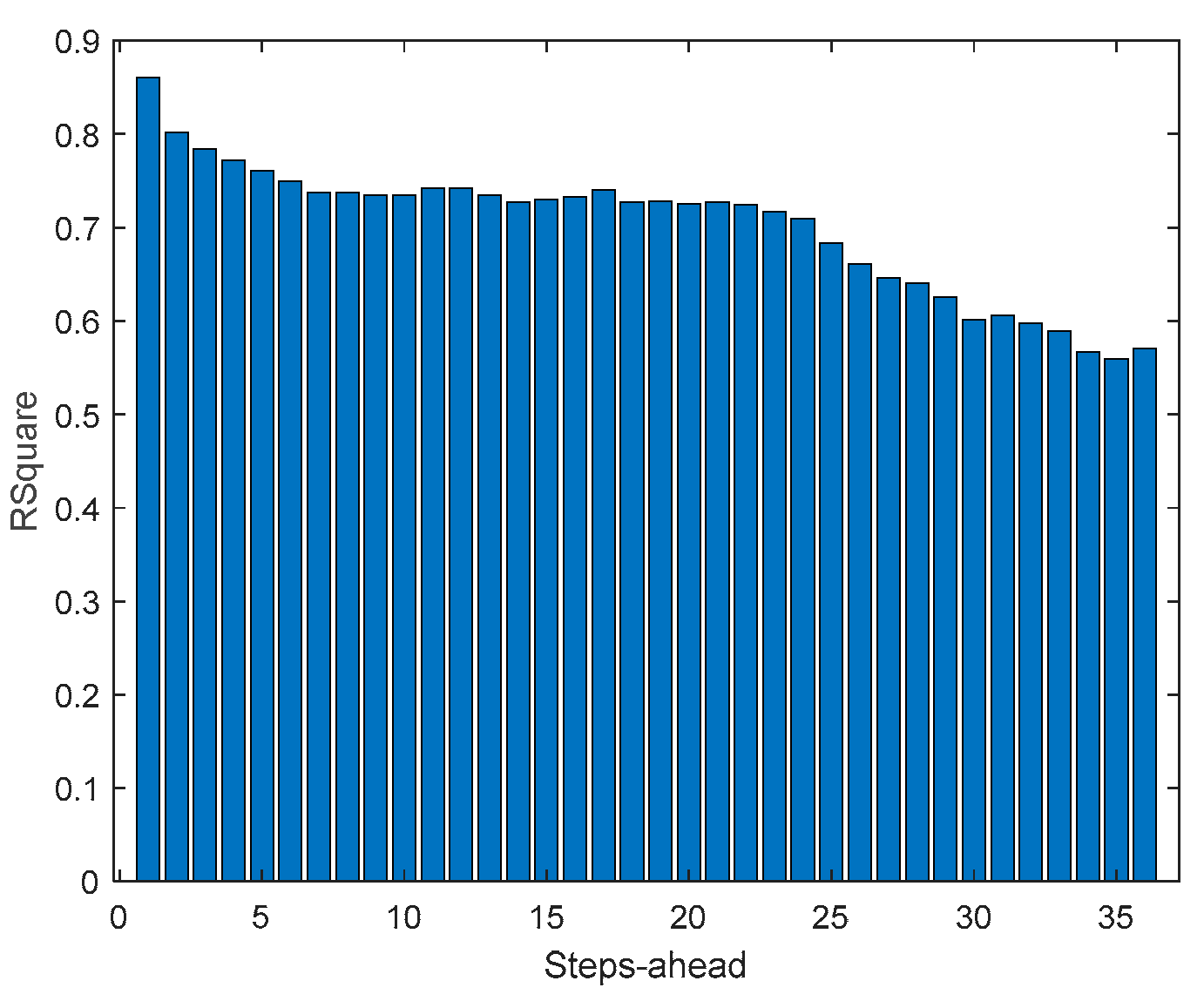
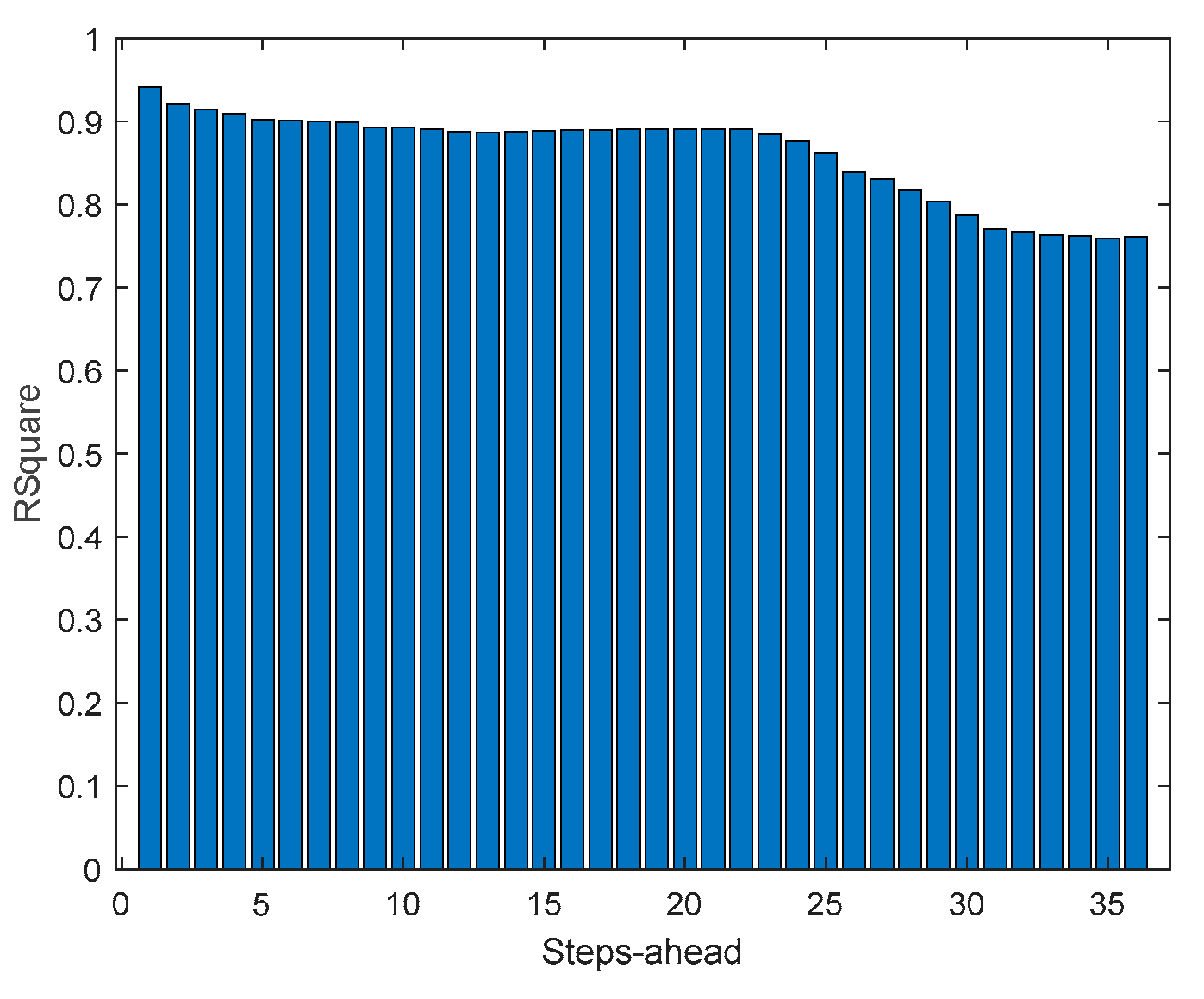
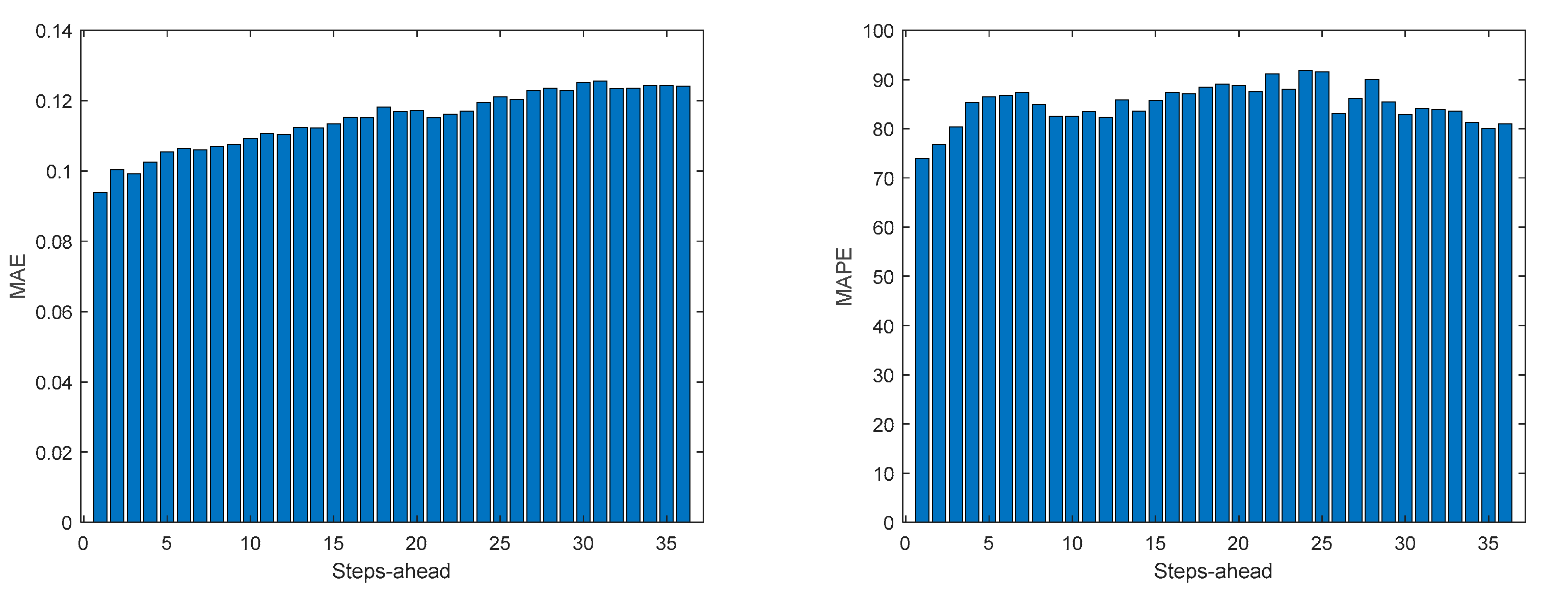
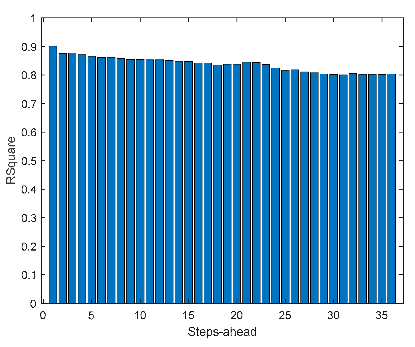
The RMSE, MAE, and MAPE change also along PH, typically increasing with the steps-ahead. However, this increase is not high and even sometimes decreases. Analyzing the evolution of the R
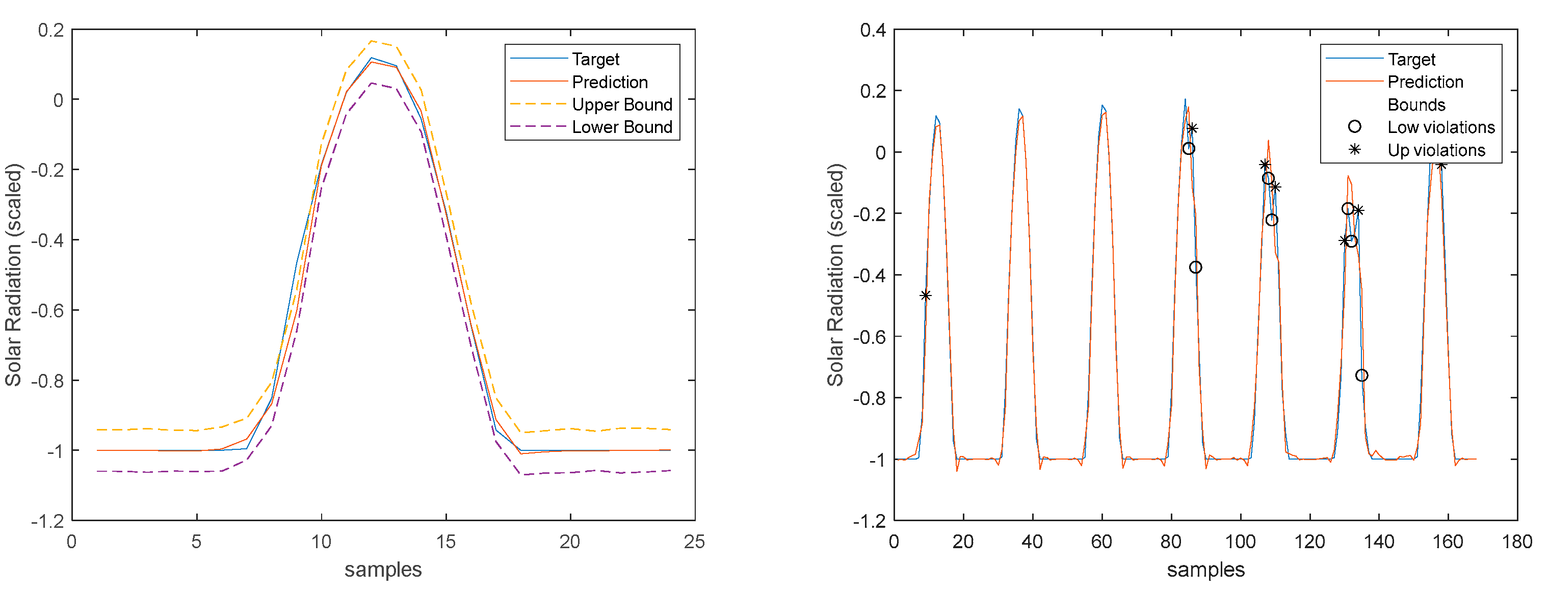
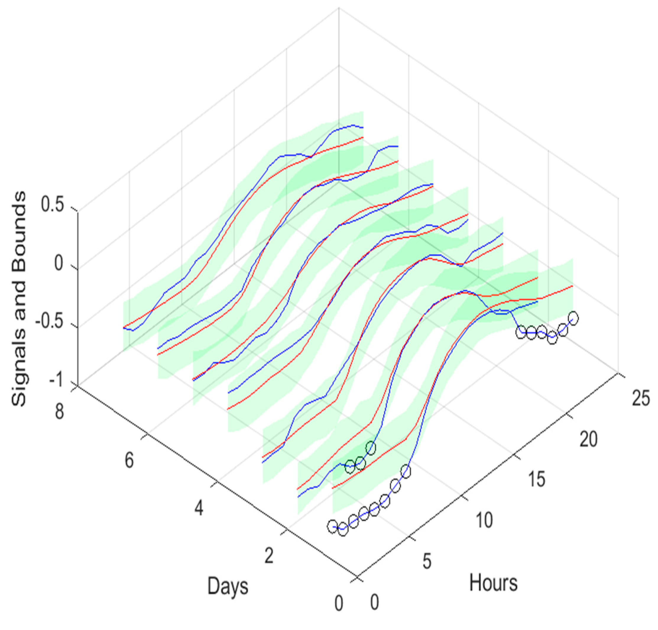
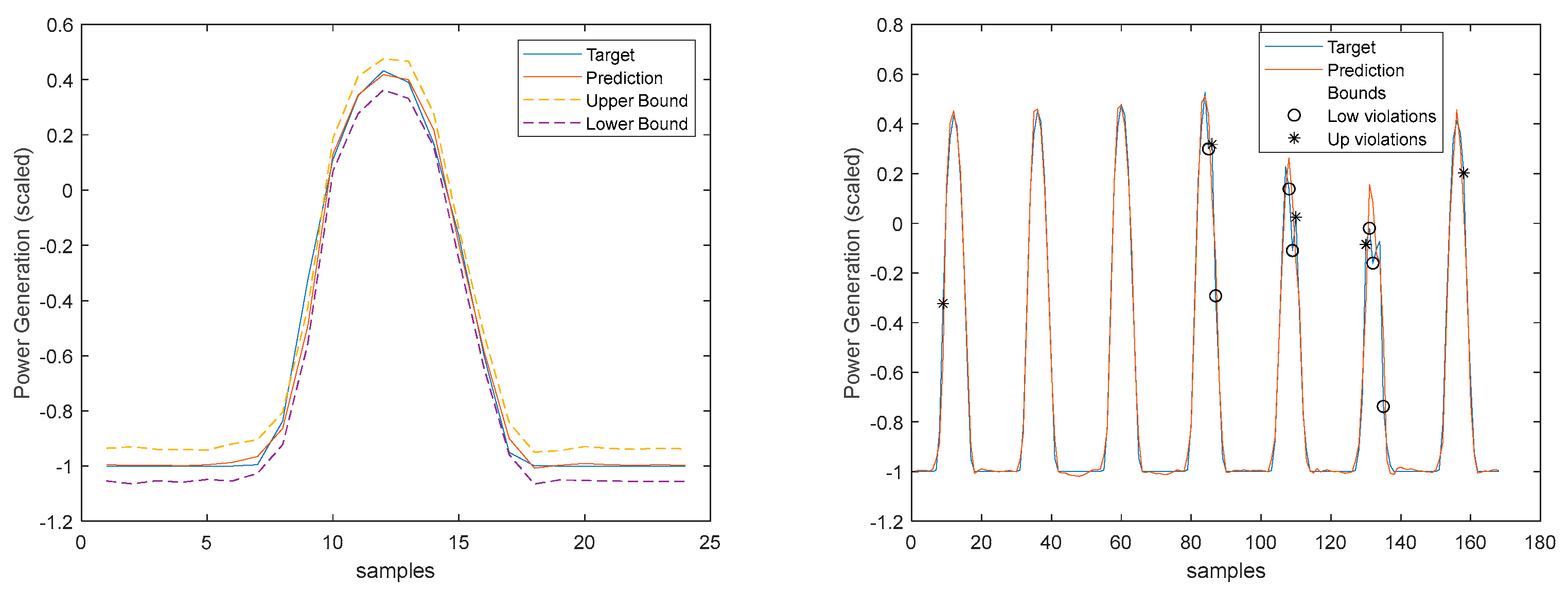
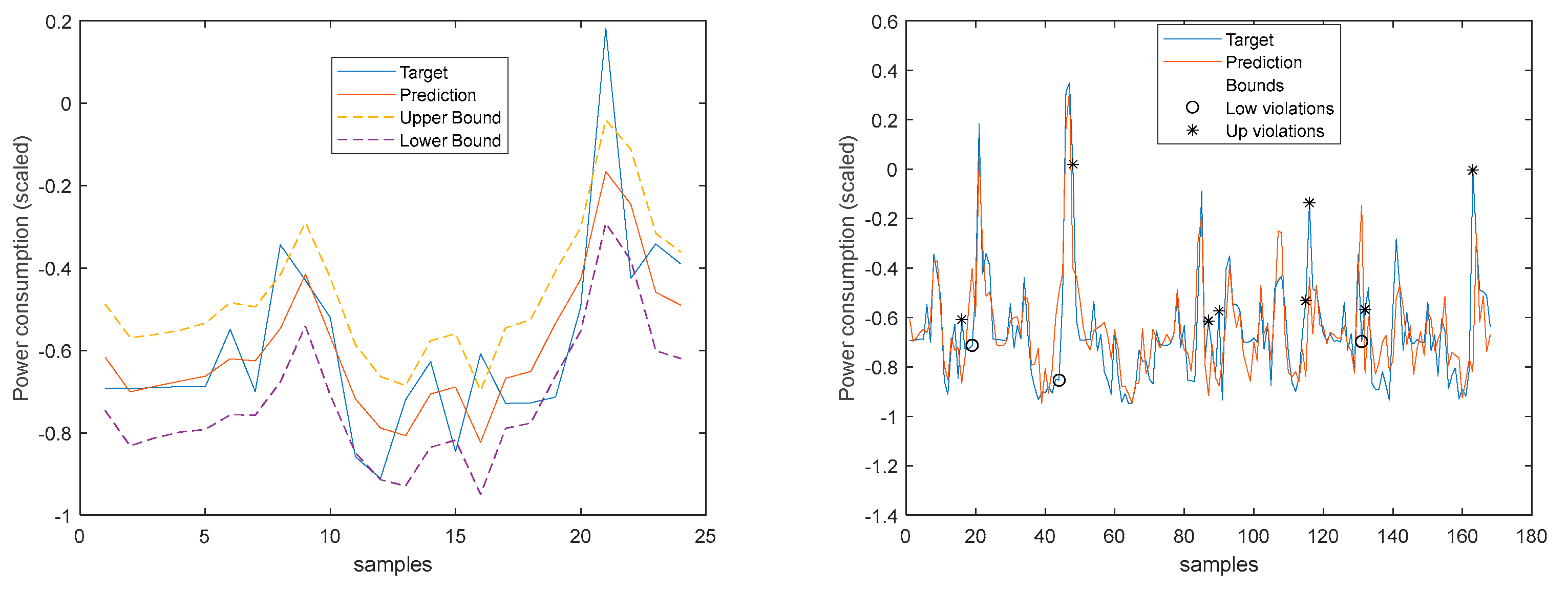
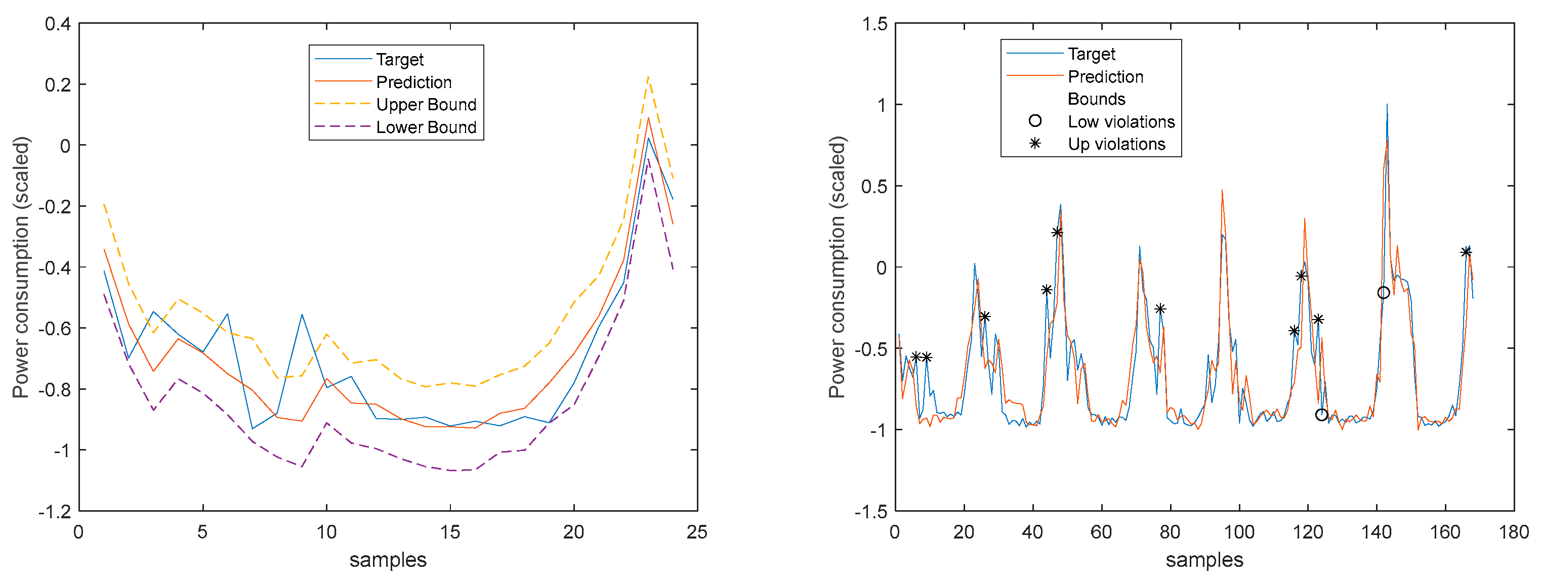
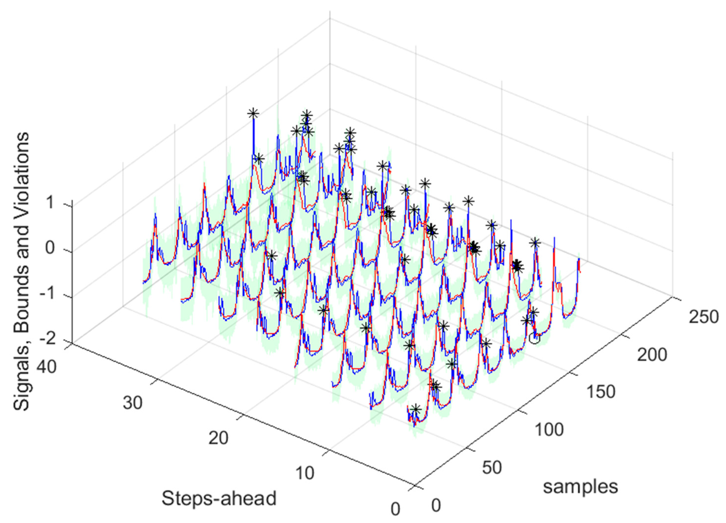
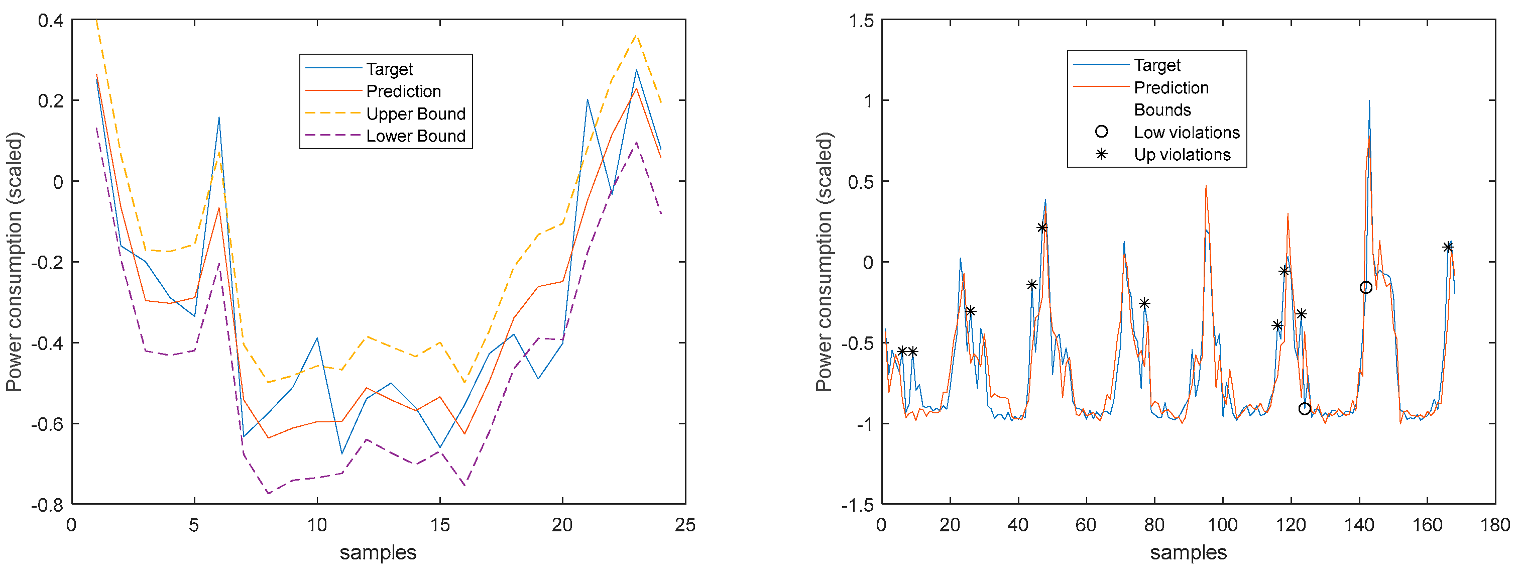
2, we can see that an excellent fit is obtained and maintained throughout the PH. This can be also seen in Figs 15, left and right. The right figure enables to confirm that the excellent performance is maintained through the PH, both in terms of fitting as well as prediction bounds and violations. Finally,
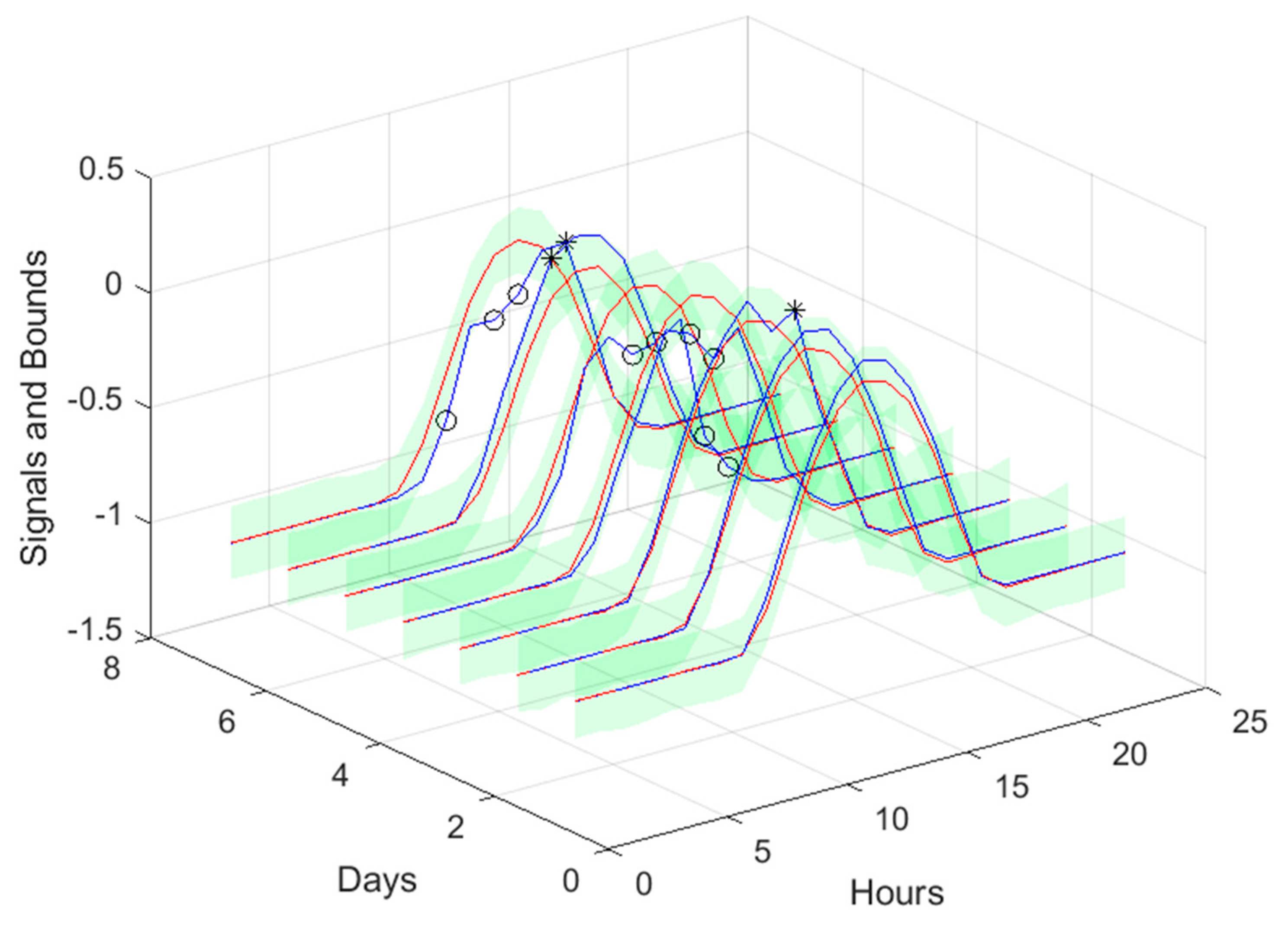
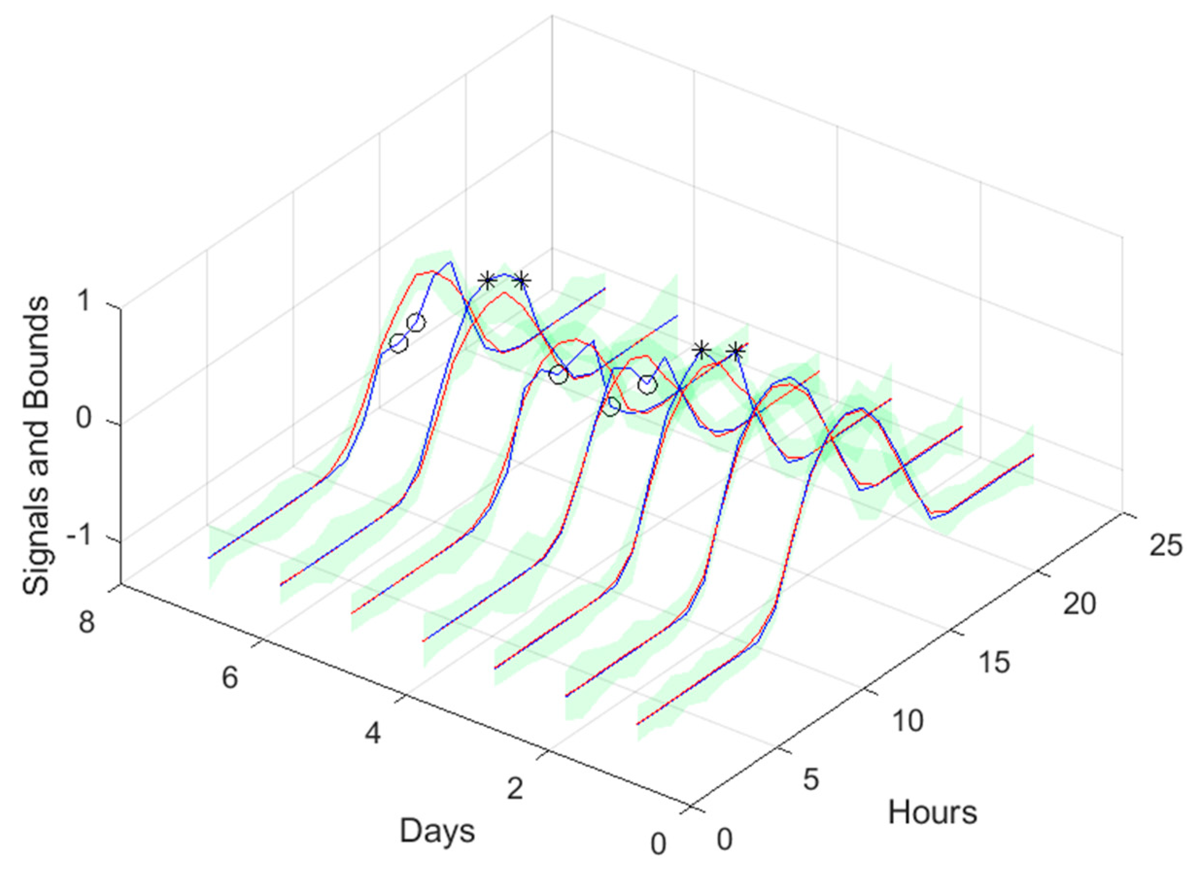
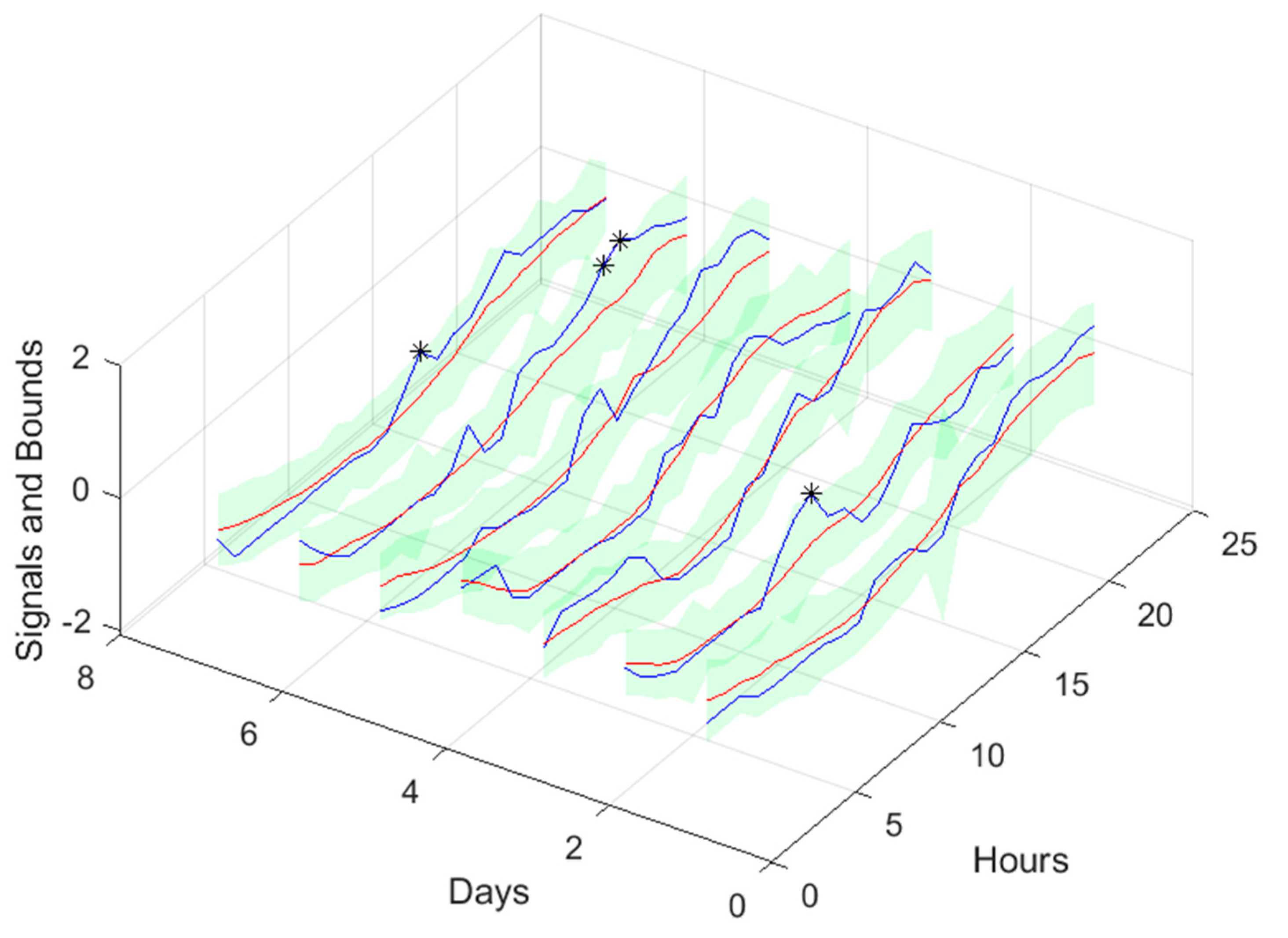
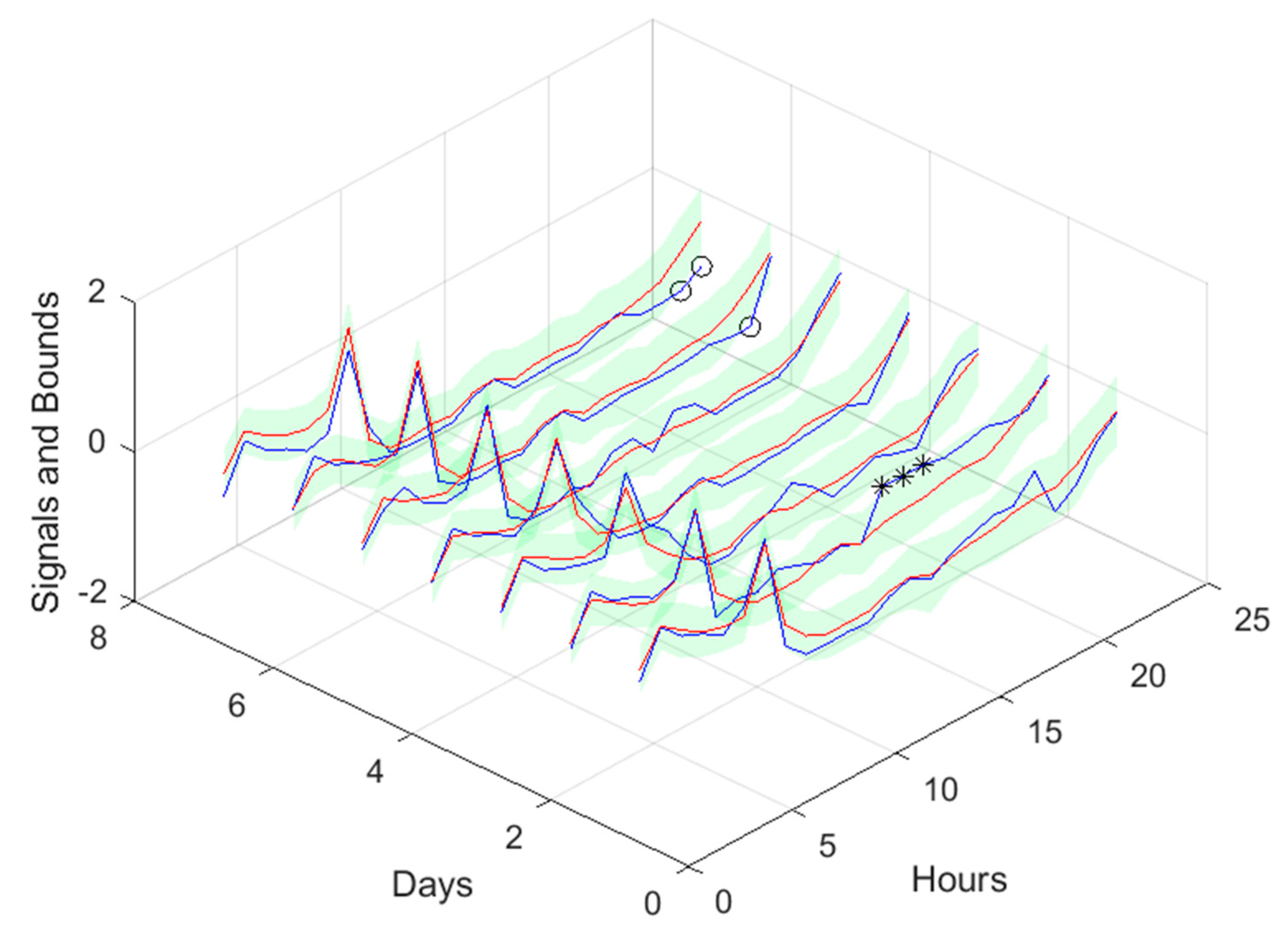
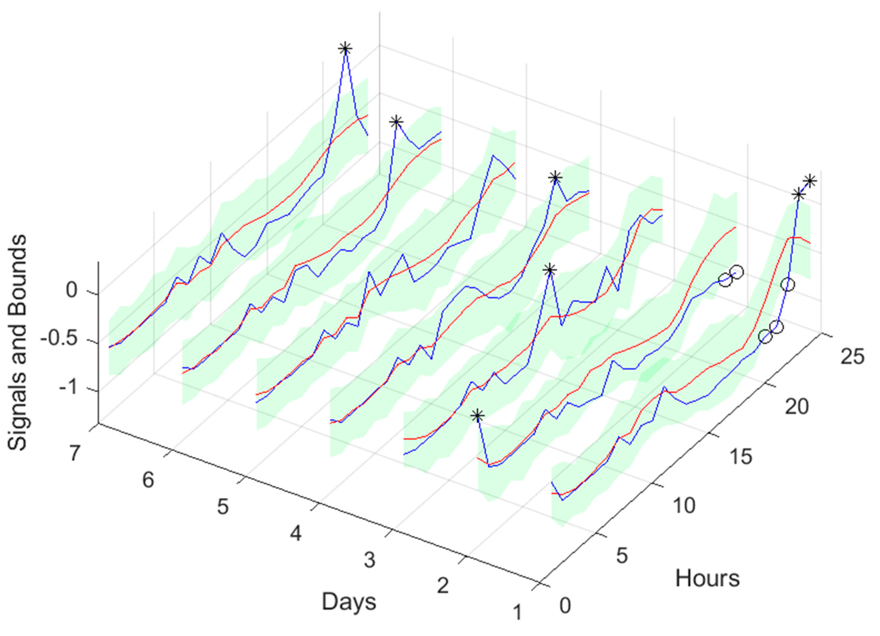
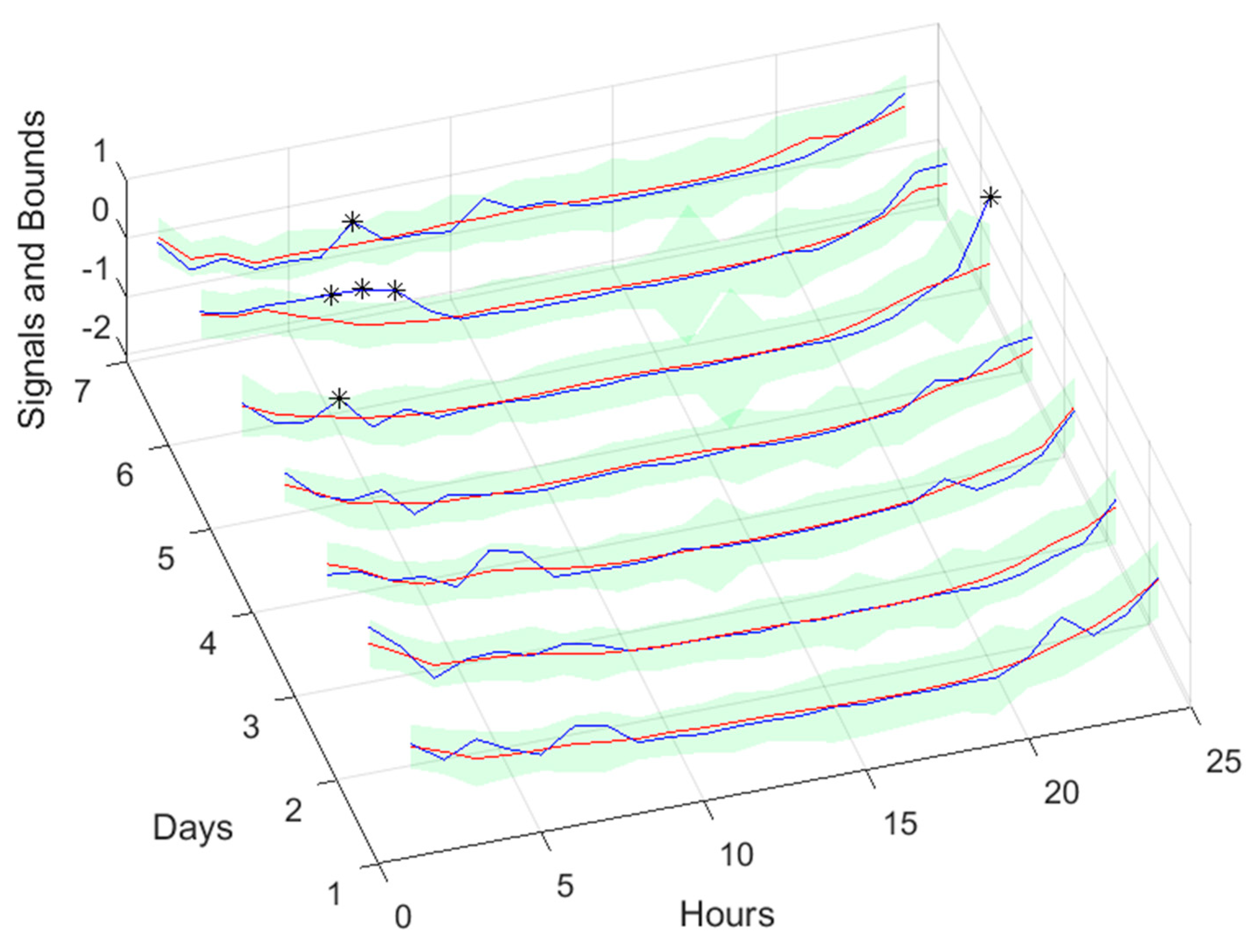
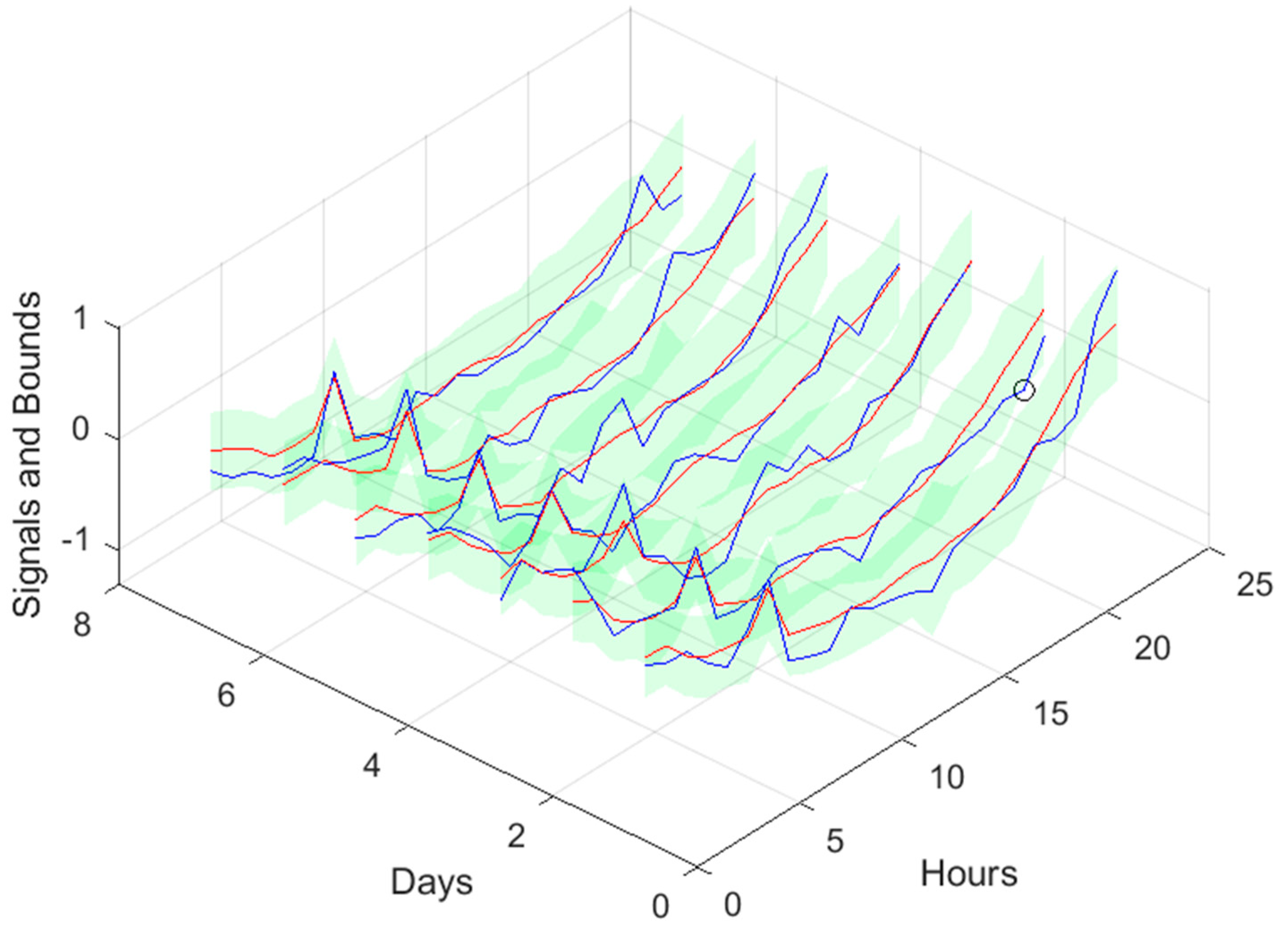
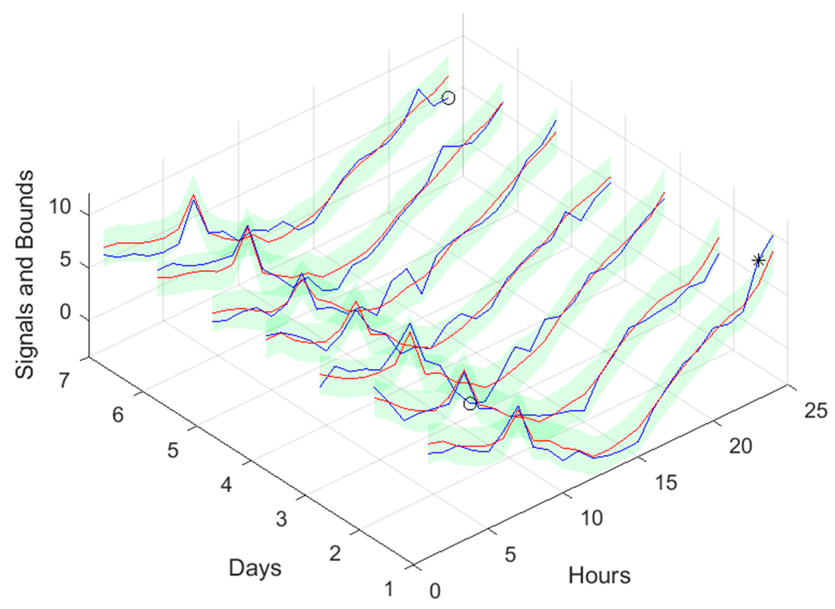
Figure 17 is focused on our goal, which is to inspect the day-ahead predictions obtained with data obtained up to 12h the day before. As it can be seen, only twelve small violations were verified, which results in a PICP of 93% in those 7 days.
3.3. Atmospheric Air Temperature models
Air temperature is also a NAR model.
Table 3 shows statistics, corresponding to the mean of the employed performance criteria, averaged over the Prediction Horizon. The evolution of the performance criteria can be seen in
Appendix A.1.
If
Table 3 is compared with
Table 2, as well as
Figure 10,
Figure 11,
Figure 12,
Figure 13 and
Figure 14 with Figures A.1.1–A.1.5, it can be observed that every performance index, apart PICP, are worse for the air temperature. One reason for this behavior might be that the solar radiation time-series is much smoother than the atmospheric temperature or, in other words, the latter has more high frequency content. This can be confirmed by examining
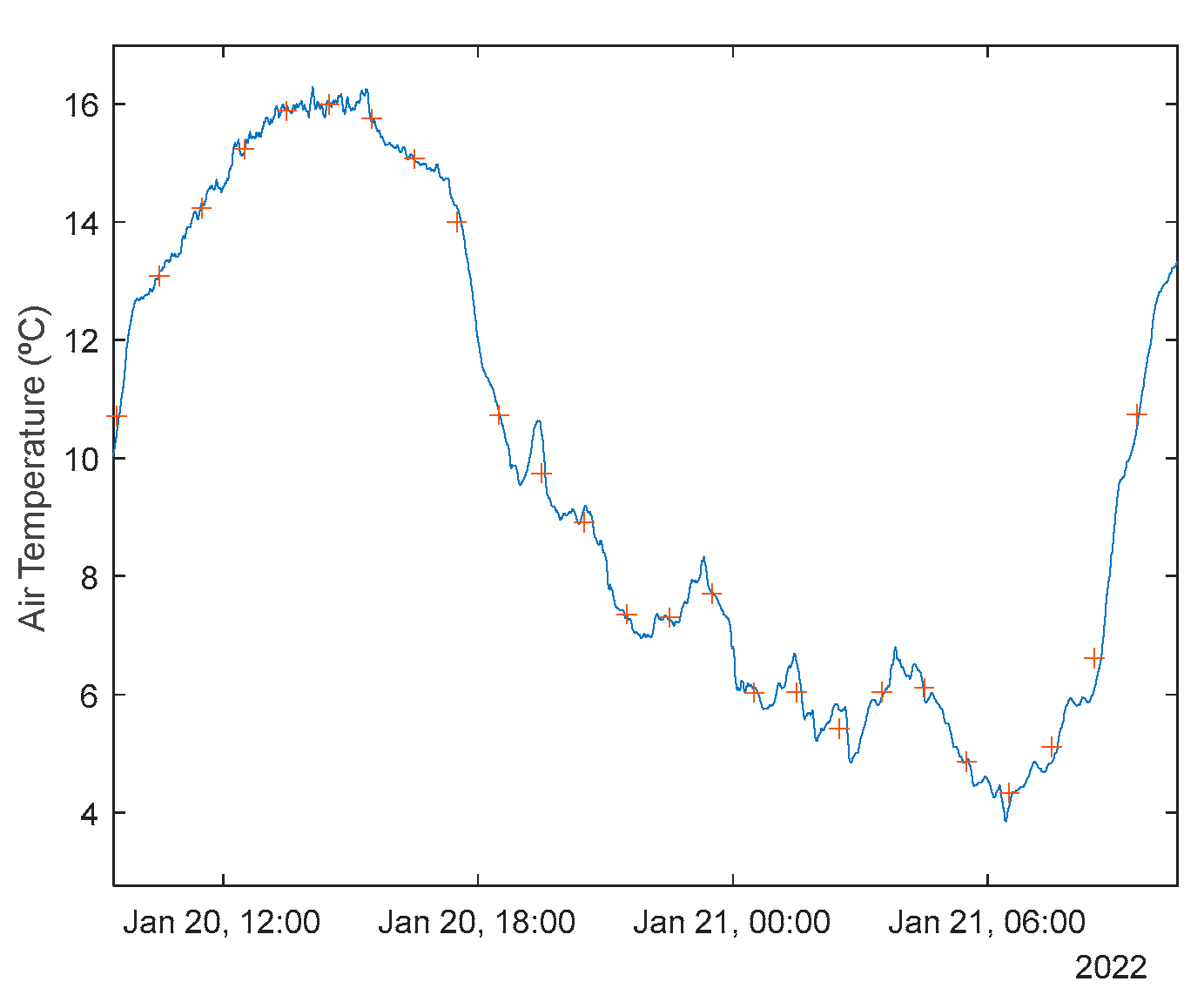
Figure 18, which presents a snapshot of the air temperature snapshot.
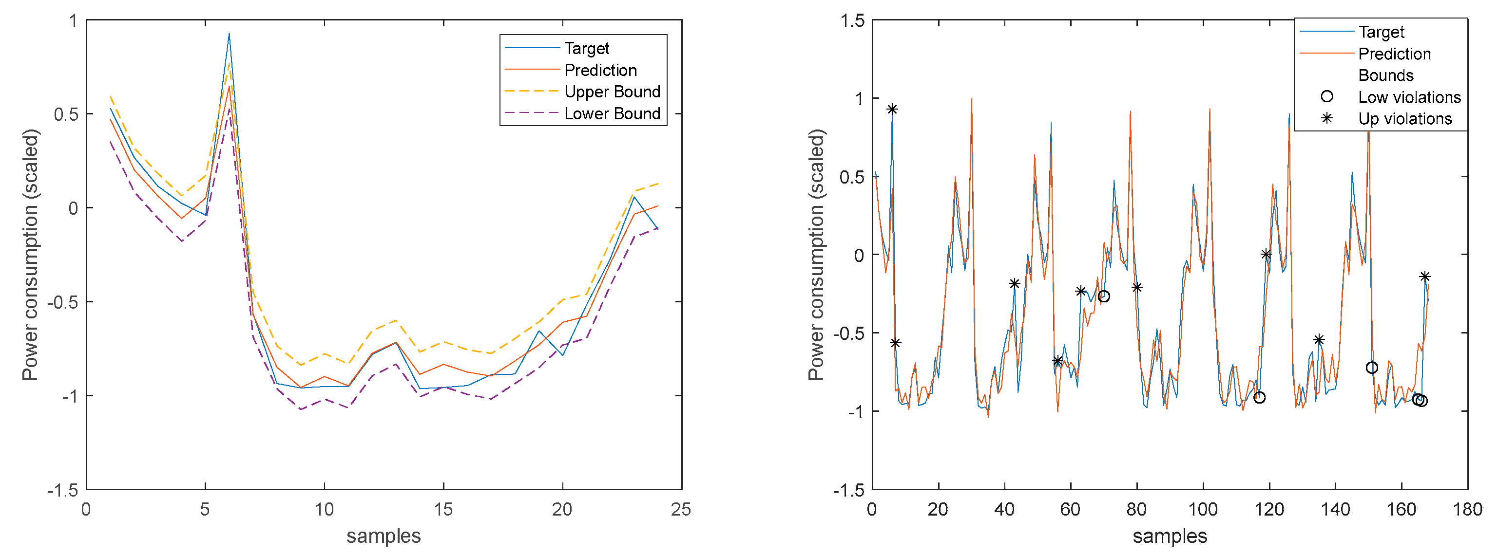
The blue line represents the time-series, sampled at 1 sec, and the crosses the 1-hour averages. It is clear that there is a substantial high-frequency content in the time-series. The 1-step-ahead forecasted signals are presented in
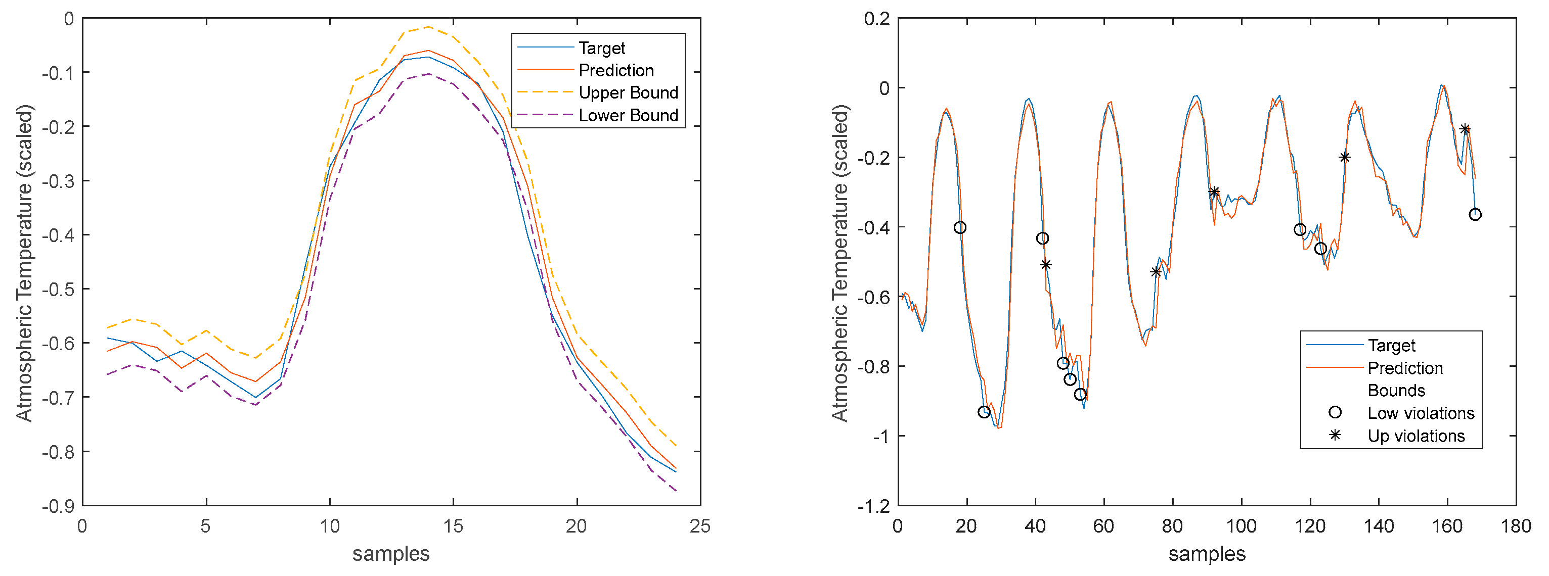
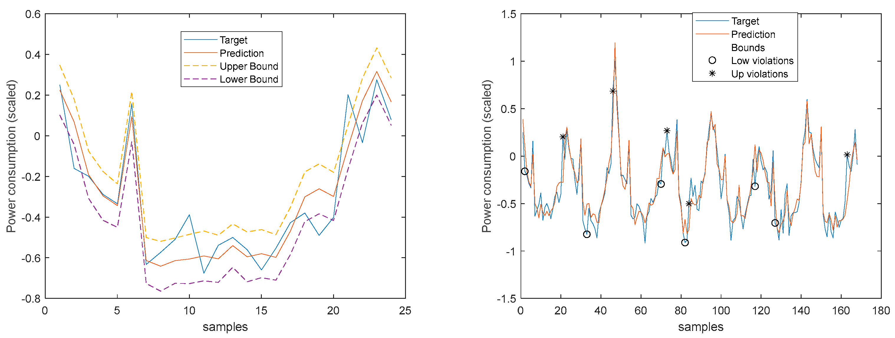
Figure 19. Looking at the right graph, only seven violations are present, corresponding to a PICP of 95%.
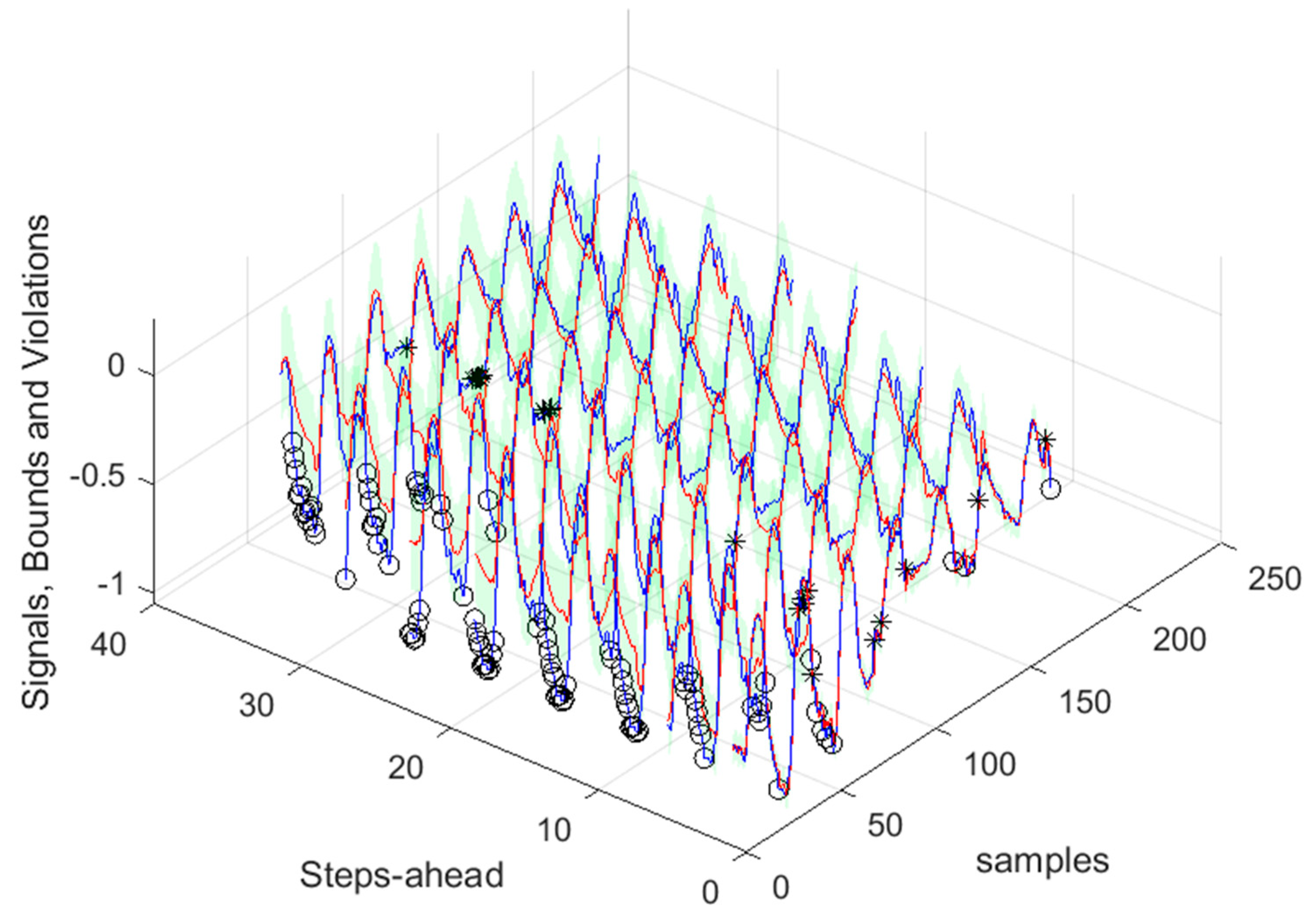
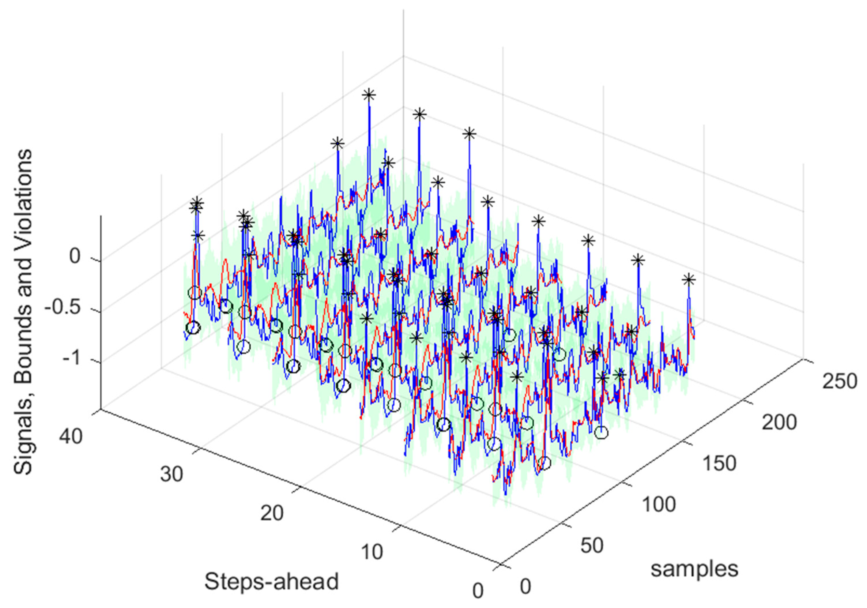
Looking at the number of violations for the steps-ahead shown in
Figure 20, the number of violations remains nearly constant with PH. The next figure shows the air temperature next day forecast.
3.4. Power Generation models
Power Generation is a NARX model.
Table 4 shows same statistics, corresponding to the mean of the employed performance criteria, averaged over the Prediction Horizon. The evolution of the performance criteria can be seen in
Appendix A.2.
The results of the power generation are similar (actually slightly better) to the solar radiation performance, as the most important exogeneous variable for power generation is really the solar radiation.
3.5. Load demand models
These are NARX models. First, we shall address the load demand of each house individually. Then, using the four models, the load demand of the community using (47) will be evaluated. Finally, the community load demand with only one model, using (48), will be considered.
3.5.1. Monophasic House 1
Table 5 shows same statistics, corresponding to the mean of the employed performance criteria, averaged over the Prediction Horizon. The evolution of the performance criteria can be seen in
Appendix A.3.
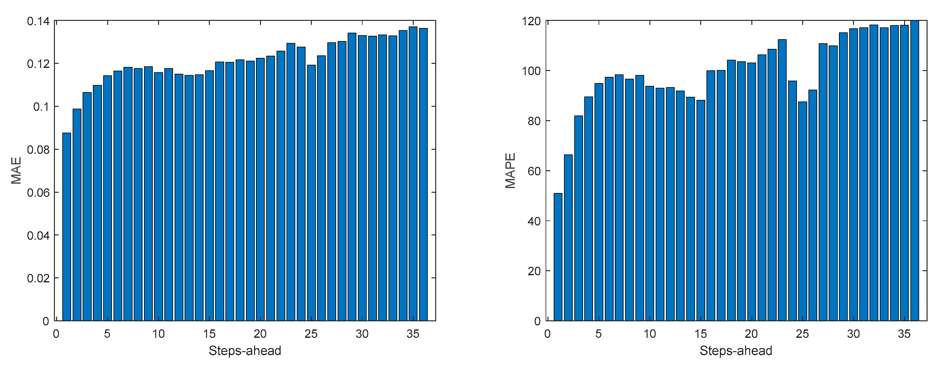
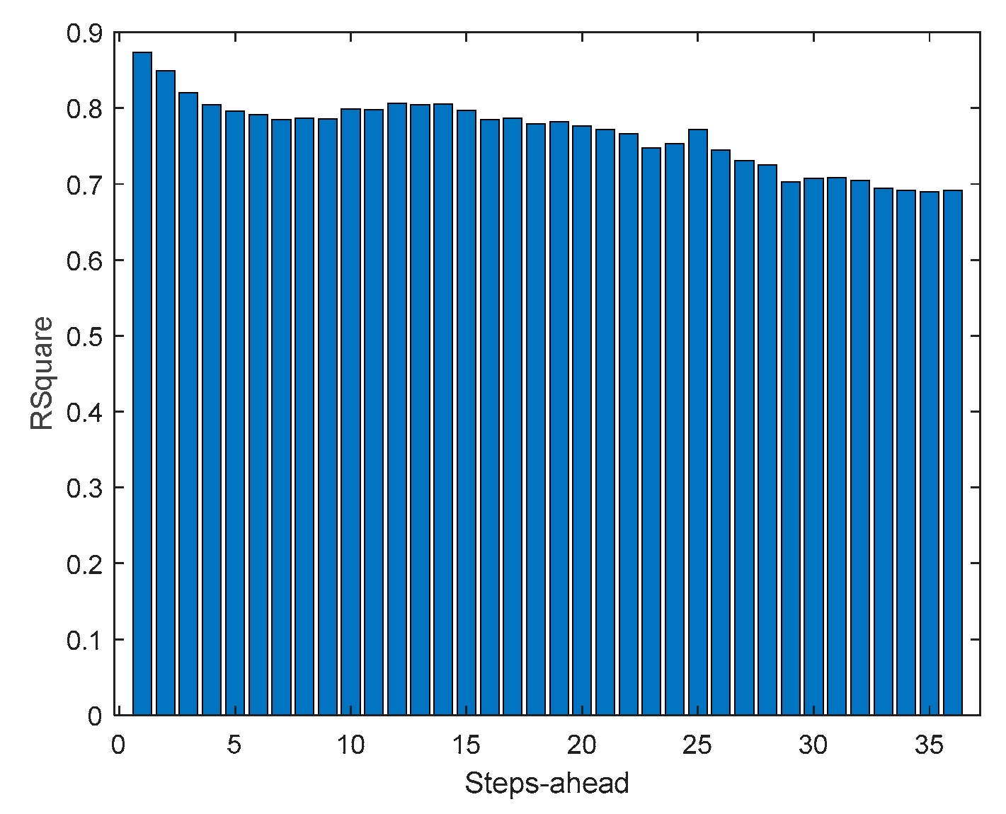
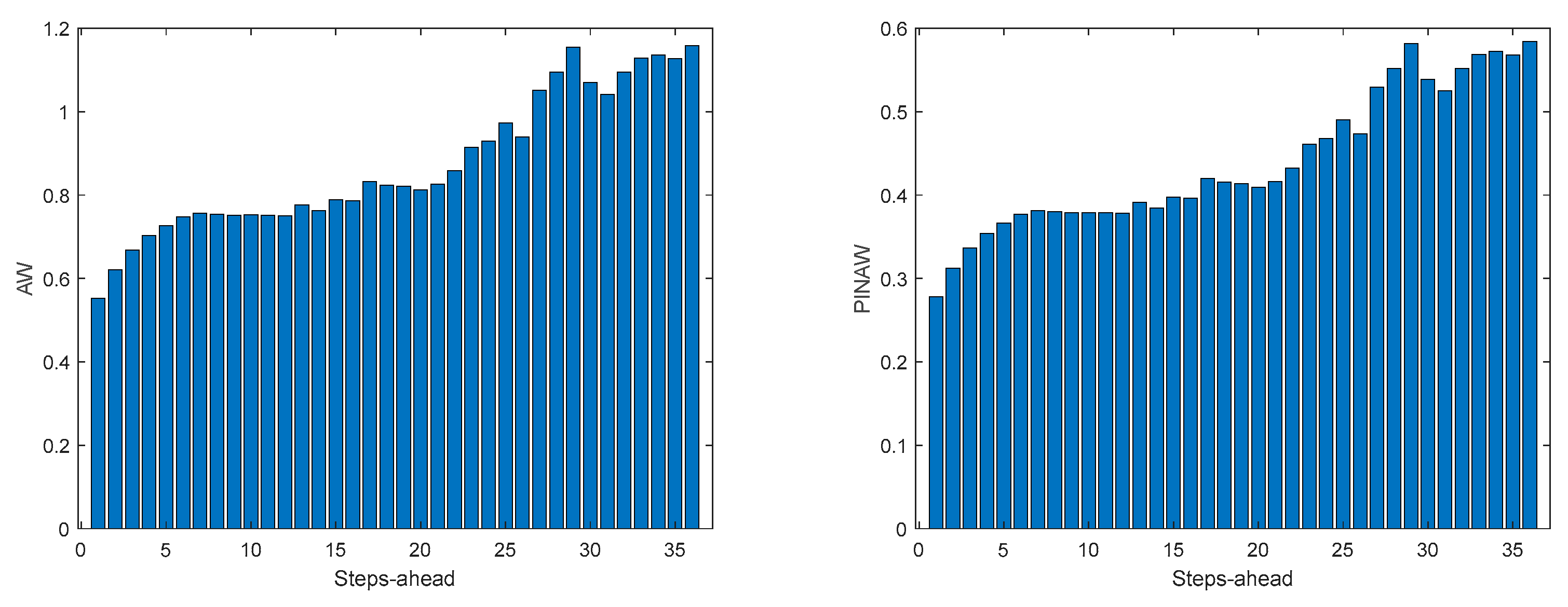
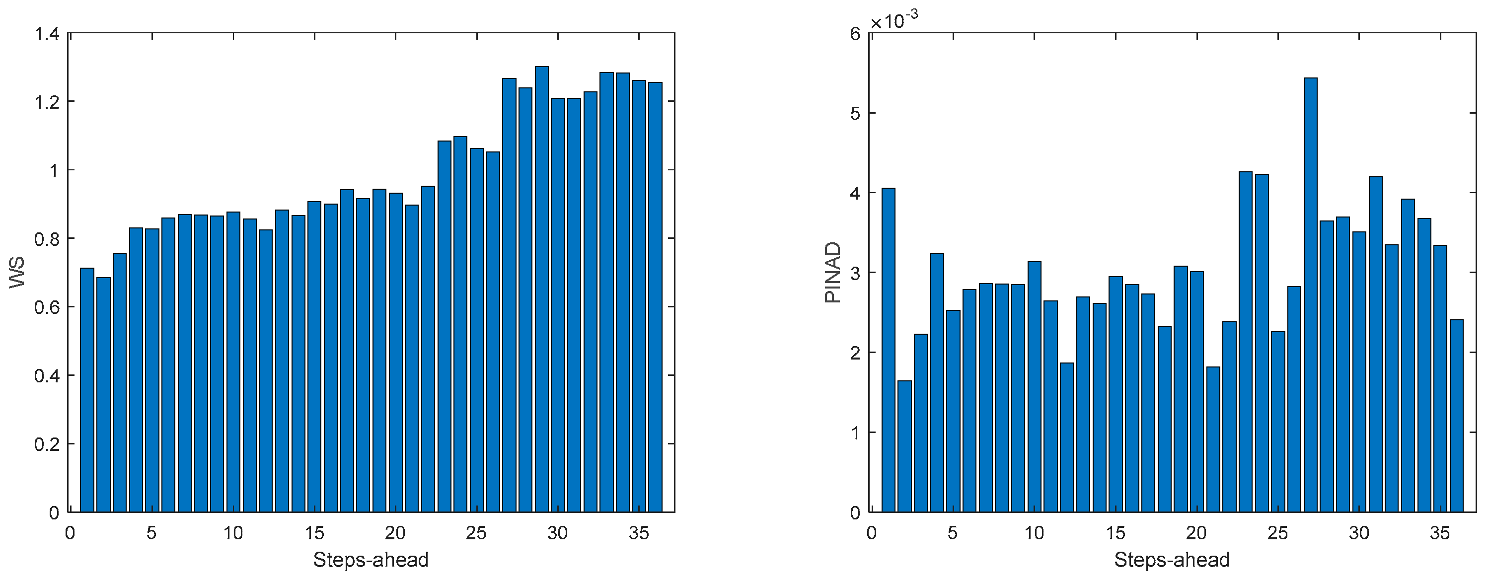
The load demand for house 1 (and as it will be shown latter, for all houses) obtains the worse results both in terms of fitting and in terms of robustness. To be able to maintain the PICP around (actually above) 0.9, the average width increases dramatically (please see
Table 5 and figures in
Appendix A.3). In contrast with the other variables analyzed before, the Winkler score is close to AW, which means that the penalties due to the width of the violations do not contribute significantly to WS.
The load demand time-series of just one house is quite volatile, as the electric appliances are a) not operated every day and b) not used with the same schedule. For this reason, it is exceedingly difficult to obtain good forecasts.
3.5.2. Monophasic House 2
Table 6 shows same statistics, corresponding to the mean of the employed performance criteria, averaged over the Prediction Horizon. The evolution of the performance criteria can be seen in
Appendix A.4.
Comparing the results of MP2 with MP1, the latter has a better performance. The average interval widths are smaller, although the average value of WS is similar, as it increases significantly along PH. The fitting is also better for MP2.
3.5.3. Triphasic House 1
Table 7 shows same statistics, corresponding to the mean of the employed performance criteria, averaged over the Prediction Horizon. The evolution of the performance criteria can be seen in
Appendix A.5.
The same comments for last case are applicable to TP1. It should be noticed, however, that the fitting () is much worse.
3.5.4. Triphasic House 2
Table 8 shows same statistics, corresponding to the mean of the employed performance criteria, averaged over the Prediction Horizon. The evolution of the performance criteria can be seen in
Appendix A.6.
The same comments for TP1 are applicable to TP2. It should also be noticed that the fitting () of TP2 is much better.
3.5.5. Community using (47)
Assume, without loss of generality, that our energy community has only two houses, whose loads are represented as
and
. We know that:
Where
Cov denotes the covariance between two signals. As it has been found that the four loads are not cross-correlated, we shall assume:
The standard error of the fit at
is given as:
For the case of two houses:
And using
the standard error of the fit at
is given as:
Please note that in (54)-(56), the selected models for the houses change with each sample. To compute the bounds, (24) and (25) must be changed accordingly.
Table 9 shows same statistics, corresponding to the mean of the employed performance criteria, averaged over the Prediction Horizon. The evolution of the performance criteria can be seen in
Appendix A.7.
3.5.6. Community using (48)
Table 10 shows the same statistics, corresponding to the mean of the employed performance criteria, averaged over the Prediction Horizon. The evolution of the performance criteria can be seen in
Appendix A.8.
The results obtained with this approach are significantly better than using (47). Additionally, there is no need to design one ensemble model for each house in the community, which can be cumbersome if there are several households in the community. If we compare the values of
Table 10 with
Table 5,
Table 6,
Table 7 and
Table 8, we can verify that in all indices the community load demand is better than each house separately. The volatility of the time series reduces when the time series of several houses are combined and, in principle, this volatility will reduce proportionally to the number of households in the community.
3.6. Net Load Demand Day-Ahead
Making use of the forecasts obtained for the community load demand, computed with (48), and for the power generated, we are able to forecast its difference, indicating the power that needs to be bought by the community (positive difference values) or sold by the community (negative values), together with the corresponding prediction bounds.
In the previous sections scaled values have been used, to enable the performance values to be compared. Here, we need to use the original values.
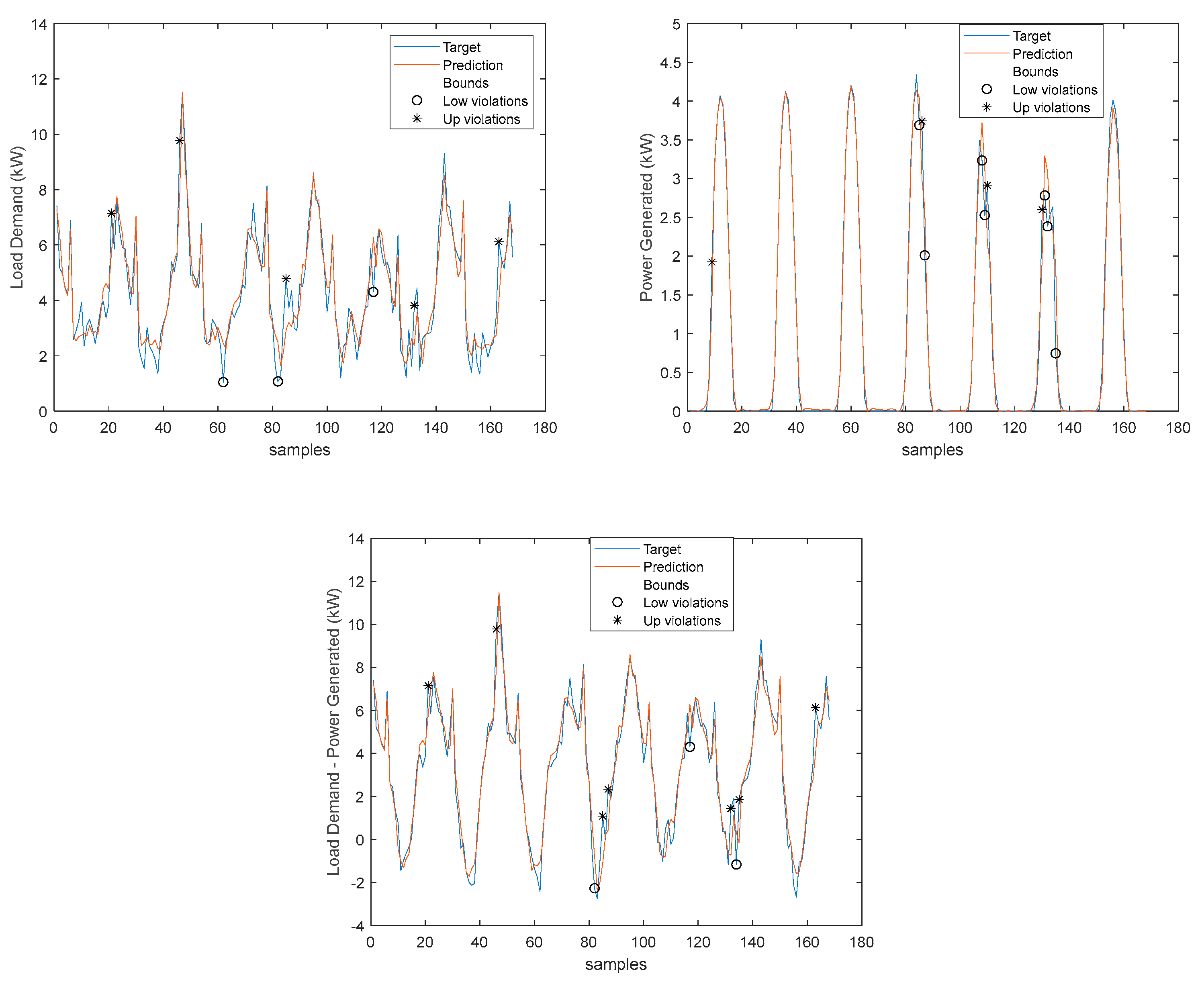
The next figures show these values for the prediction time-series, where the lower bounds for both the load demand and power generated have been adjusted to ensure that power stays always positive.
As we shall be interested in forecasts between 13 and 36 steps-ahead (the next day values obtained at 12’o clock the current day), the next results will only consider this range of steps-ahead.
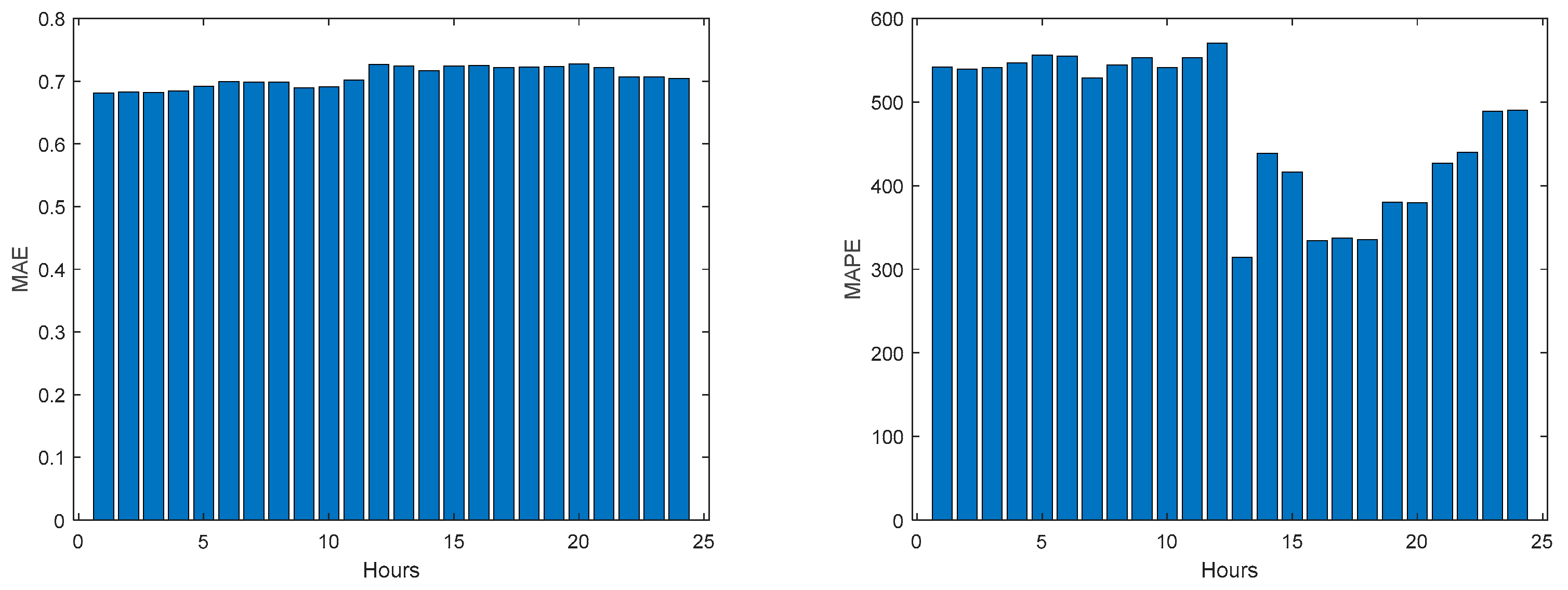
Please notice that as the Net Load has a substantial number of values near 0, MAPE has very large values.
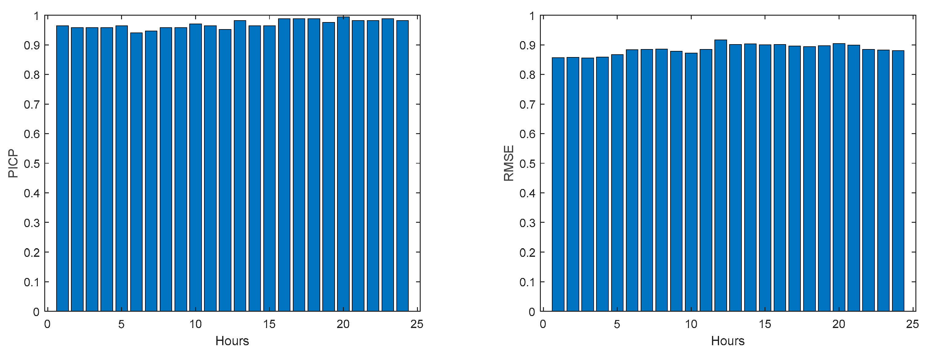
Please note that the number of upper(lower) violations is 35(17) in a total of 1512 samples, which results in a PICP of 0.97.
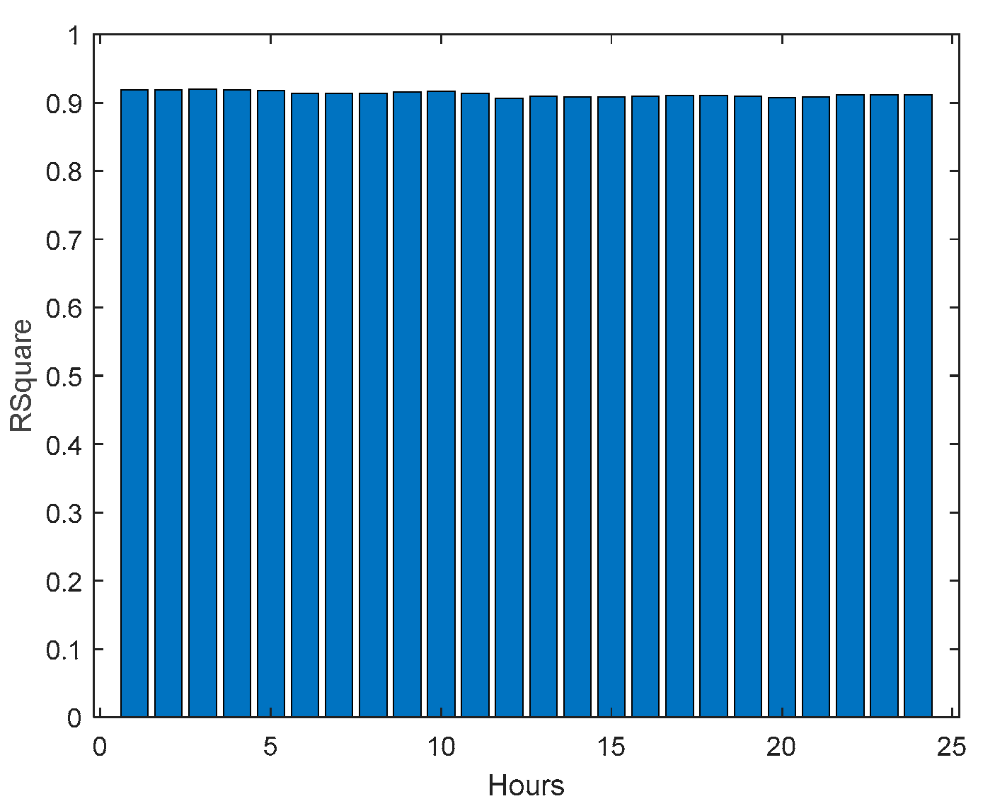
There is one upper violation and two lower violations, resulting in a PICP of 0.98. As it can be seen, there is a particularly good fitting (R2 values above 0.9), and the values are not so high, with an average value of 0.28, which is significantly smaller than the values obtained for the load demand of the individual houses. It is argued that for a larger energy community, or for the union of different energy communities managed by the same aggregator, the results would be superior, for the point forecasts indices as well as the robustness indicators.
4. Discussion
Analyzing the results presented above it can be concluded that the design procedure described in
Section 2.2, together with the procedures described in
Section 2.4 and 2.5, produce accurate models with a value of PICP almost constant throughout the prediction horizon. The average values, presented in
Table 2,
Table 3,
Table 4,
Table 5,
Table 6,
Table 7,
Table 8,
Table 9,
Table 10 and
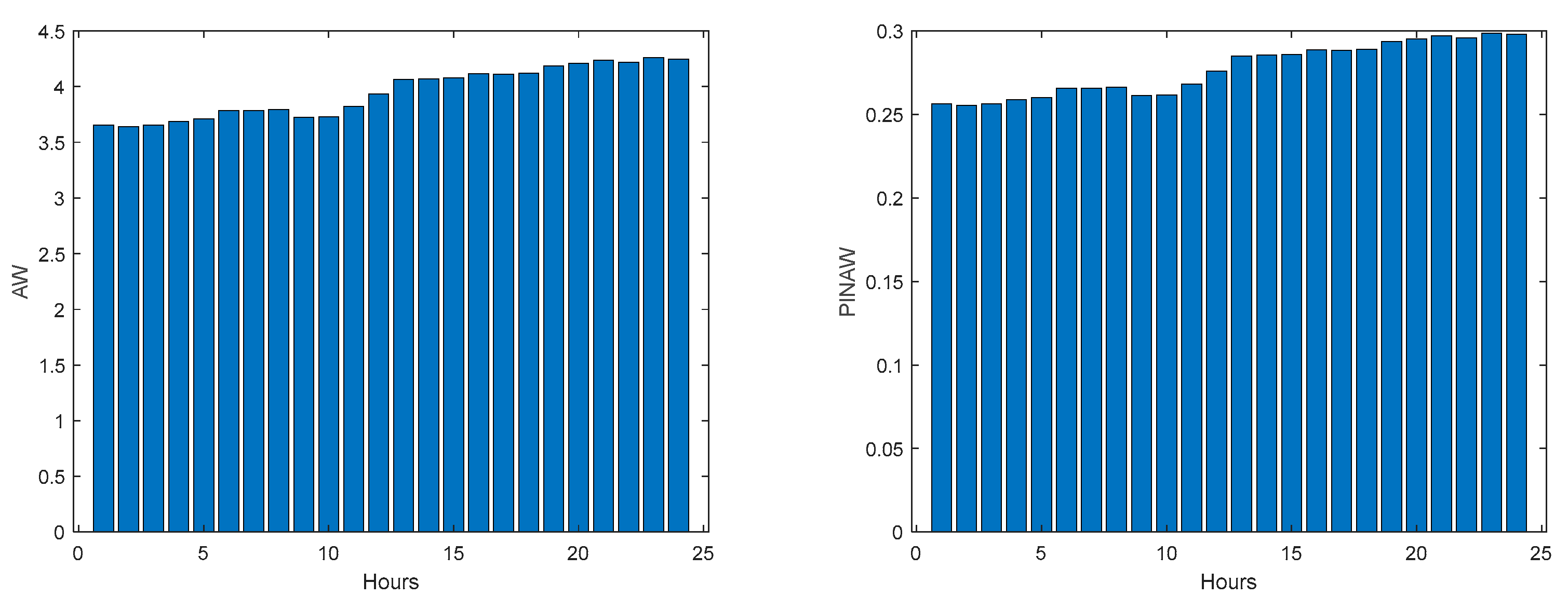
Table 11 are always higher than the desired confidence value of 0.9. For the evolution of the day-ahead net demand in the 7 days chosen, a PICP value of 0.98 is obtained, with an average value of PINAW of 0.28. As there is a trade-off between PICP and AW, a smaller value of PINAW could be obtained by slightly decreasing PICP.
In what concerns the rest of the performance indices, in most cases they increase with PH (except for R2, which decreases), as expected. But the increase (decrease) rate is not so high, which means that the forecasts are still useful for the day-ahead. This behavior changes for the net load demand, as the performance indices are almost constant throughout the next day.
To assess the quality of the results, they should be compared with alternatives found in the literature. It is difficult to compare them quantitatively with rigor as, on one-hand, only one publication cold be found for day-ahead net load demand and, on the other hand, the contexts of the works in comparison are different between themselves and between this work. With those remarks in mind, we shall start by works that were briefly discussed on the introductory section on load demand, and afterwards on power generation.
Kychkin et. al. [
17] employ data from 4 houses located on Upper Austria. They compute at the end of one day the prediction for the next 24 hours, with a 15 min sampling interval. Notice that in our case we forecast the load demand for 36 hours ahead, with a sampling interval of one hour. When the simulation period extends for several days, at the end of each day the models are retrained with data available until that time. In our case, the models remain constant. For a simulation period of one week, which is equal to this paper, they obtain a normalized RMSE of 0.995 for the best single model, and 0.96 for the best ensemble model. In our case, and using (48), a
of 0.15 is obtained, with scaled data. Assuming that the NRMSE is computed as (the paper does not clarify that):
We obtain a NRMSE of 0.19. This value is smaller than the values obtained in the discussed paper even when, as pointed out, their model is retrained every day, and our forecasting horizon is larger.
Vilar and co-authors [
6] employ probabilistic forecasting. As reported previously, they employ the whole Spanish load demand for year 2012, not four houses as we did. They only employ as performance criteria the Average Width (AW) and the Winkler score. Using a confidence level of 95%, the yearly weekly average width is 5,572 MW, and the Winkler Score around 8,872. The total demand value is omitted but using
Figure 1 of the paper it should be around 20,000 MW. This way, the Prediction Interval Normalized Averaged Width (PINAW) should be around 28%, comparing to 31% for our case. This way, similar PINAW are obtained, for cases that are not comparable (4 households load demand against the whole Spanish load demand). In terms of WS, if we normalize the value shown in the paper by the total demand, a figure of 0.44 is obtained, which is the same value obtained in this paper.
Zhang and co-workers [
9] use data from two cities and one region in China. The best method (MCQRNNG) for a set of 5 days obtains MAPE values of 1.61, 1.74 and 1.47 for the cities of Ottawa, Baden-Württemberg, and the China region, respectively. In our case, a value of 0.87 is obtained. Their measured PICP values were 0.88, 1, and 0.87. In our case, a value of 0.96 is obtained. Their PINAW values were 0.11, 0.14 and 0.08, while we obtain a higher value of 0.31. In the same way as in the previous paper, we are comparing whole cities and regions with just four houses.
Addressing now PV generation forecasts, [
23] used PV output power data collected by a roof-mounted PV power generation system in eastern China. The installation capacity is 2.8 MW. In our case, the capacity is only 6.9kW. They used as performance indices the Normalized MAE, computed with (58), adapted to MAE, and the Winkler score, with 90% confidence level. The average values, computed for selected 6 days in the test set, were 34.9% and 40.1. In our case we obtain 24.9% and 1.9, respectively.
The work [
19] uses data from 300 Australian houses. In each one of the houses hourly load demand and PV generation values were recorded, from 2010 to 2013. A prediction horizon of twenty-four steps is considered. Using the best model, the average RMSE and MAE for the load demand were 4.53 and 3.39, respectively. The average load demand had to be estimated from
Figure 10 of the paper and it is roughly 35kW. This is translated into normalized values of 0.13 and 0.11. Our figures are 0.19 and 0.15, with only four houses and a PH of 36 hours. In terms of PV generation, the RMSE and MAE values are 2.5 and 1.19, respectively. Estimating the average value of 11 kW using
Figure 11 of the paper, the normalized values obtained were 0.23 and 0.11. Our values 0.25 and 0.13, which are similar.
Finally, as pointed out before, paper [
24] is the only publication that has the net load forecasting as its target. It uses smart meter data collected from a residential community comprising fifty-five houses in the IIT Bombay area, with a time interval resolution of 1 hour. The only performance criterion that can be used is MAPE, for load demand and PV generation. Assuming that the values shown in the paper are for the 24 hours ahead and not for the one-step ahead, the MAPE values were 0.49 and 0.75. Our values are 0.87 and 0.54, for a thirty-six forecasting steps for load demand and PV generation, respectively. Therefore, the MAPE load demand, for the fifty houses, is better than ours, for just four houses. In contrast, our results for PV generation are better than their.
5. Conclusions
We have proposed a simple method for producing both point estimates and prediction intervals for a one-day ahead community net load demand. The prediction intervals obtained correspond to a very high confidence level (0.96) with a reasonable average Prediction Interval Normalized Averaged Width value of 0.28. As these values were obtained with a desired PICP value of 0.90, small PINAW values could be obtained by lowering the desired PICP value.
No direct comparison could be found in the literature. This way, comparisons were made indirectly, by assessing the performance of load demand and PV generation forecasting alternatives. Regarding the former, for the only case with the same number of houses considered here, our proposal obtains much better point forecasting performance. All the other works employed a significantly large number of households, obtaining typically better results. As it was demonstrated in the paper, it should be expected an improvement of results with an increase of the number of households. In relation with PV generation, our approach obtains similar or better results than the alternatives.
One point that should be stressed is that, in our approach, the forecasts are obtained by small shallow artificial neural networks, whose complexity is orders of magnitude smaller than the alternative models, that typically are whether deep models or ensembles of deep models. With the obtained results, similar or better than the competitors, it can be concluded that by employing parsimonious models, designed with good data selection, feature selection and parameter estimation algorithms, better results can be expected than employing “brute force” deep models.
For all models described in this paper, the obtained PICP values were higher than the confidence level sought. This is obviously better than the opposite behavior, but in the future, we shall look at ways of obtaining PICP values more similar to the desired confidence level.
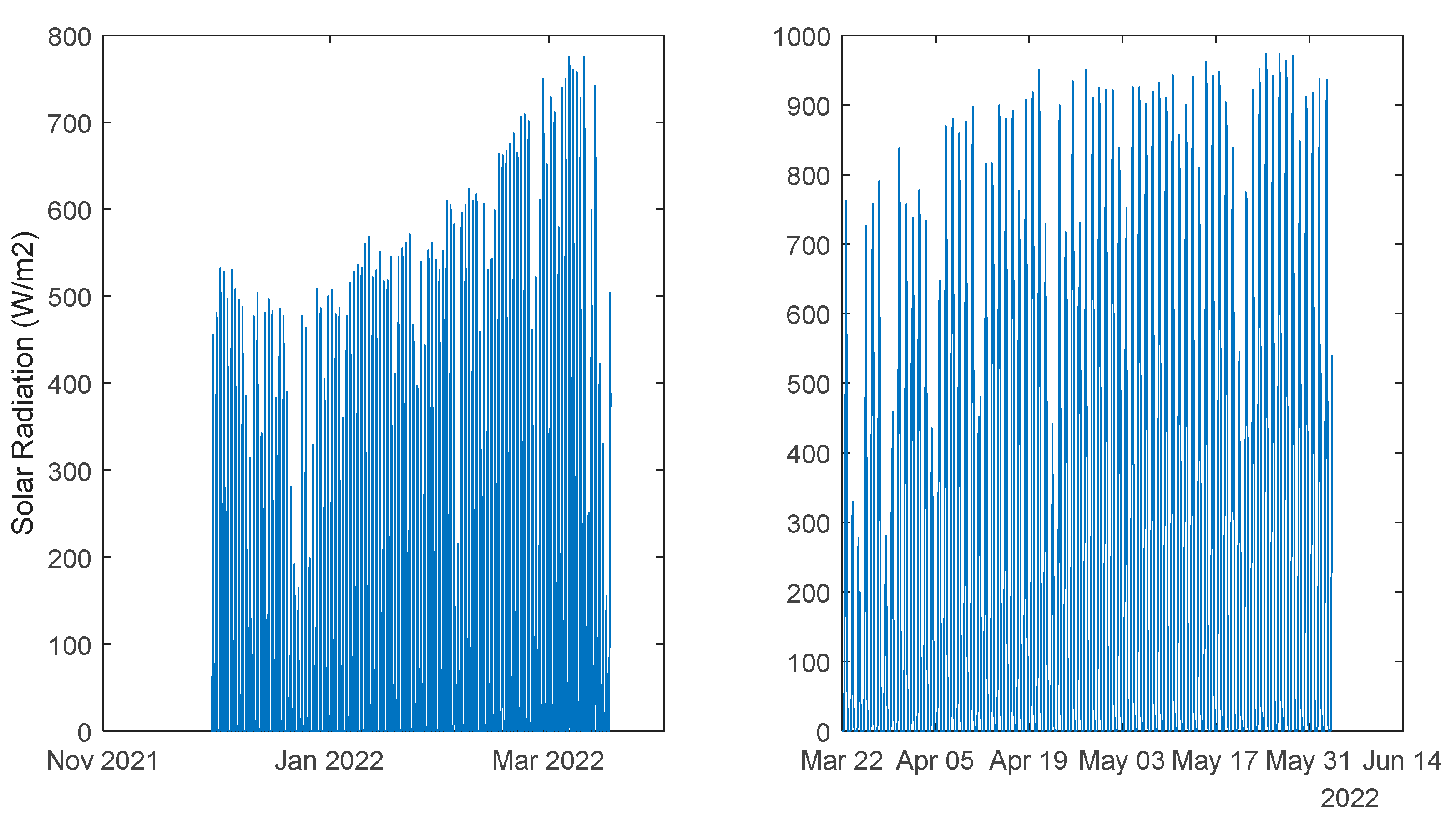
Figure 1.
Solar Radiation. Left: 1st period; Right: 2nd period.
Figure 1.
Solar Radiation. Left: 1st period; Right: 2nd period.
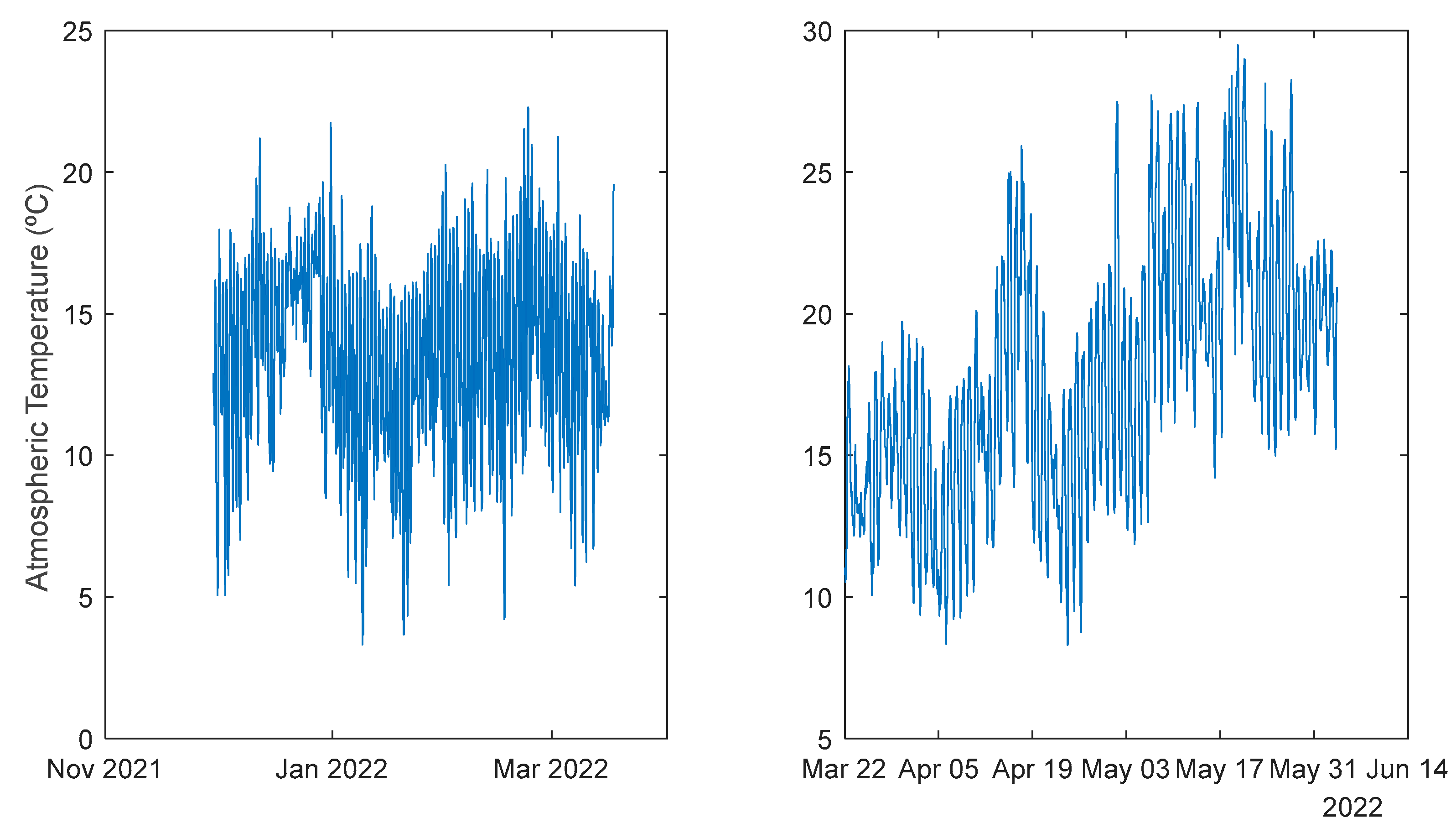
Figure 2.
Atmospheric Temperature. Left: 1st period; Right: 2nd period.
Figure 2.
Atmospheric Temperature. Left: 1st period; Right: 2nd period.
Figure 3.
Day Code. Left: 1st period; Right: 2nd period.
Figure 3.
Day Code. Left: 1st period; Right: 2nd period.
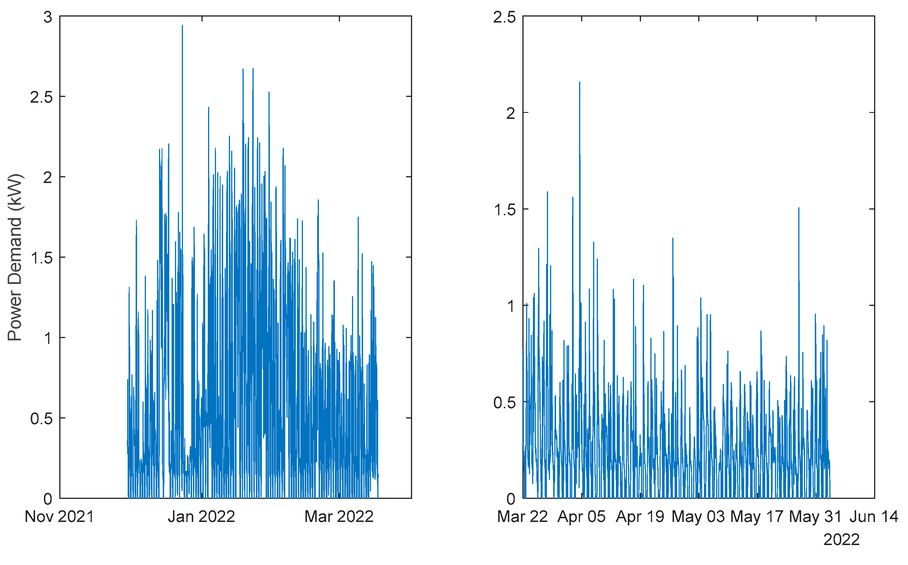
Figure 4.
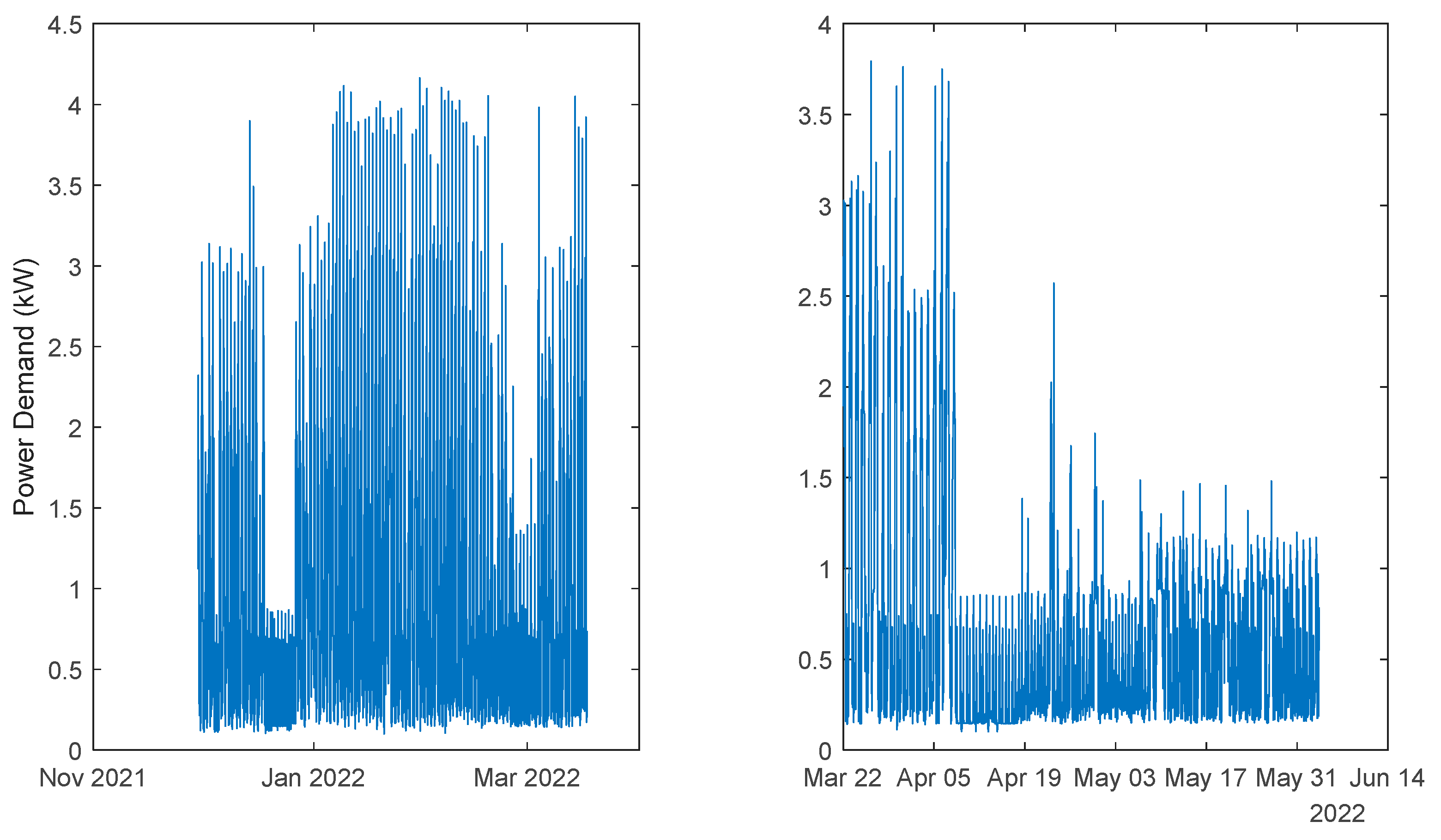
Power Demand: House 1 (monophasic). Left: 1st period; Right: 2nd period.
Figure 4.
Power Demand: House 1 (monophasic). Left: 1st period; Right: 2nd period.
Figure 5.
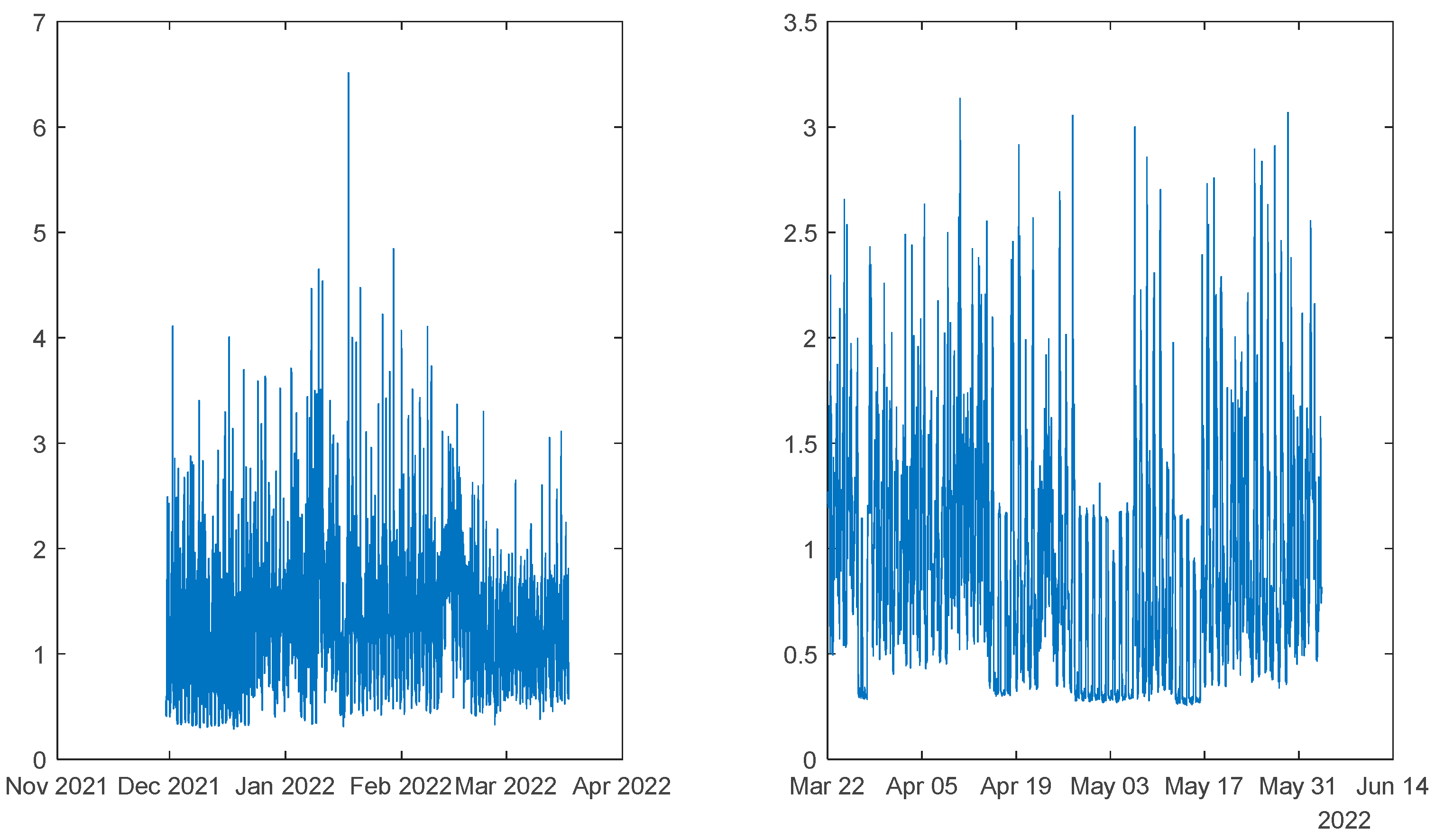
Power Demand: House 2 (monophasic). Left: 1st period; Right: 2nd period.
Figure 5.
Power Demand: House 2 (monophasic). Left: 1st period; Right: 2nd period.
Figure 6.
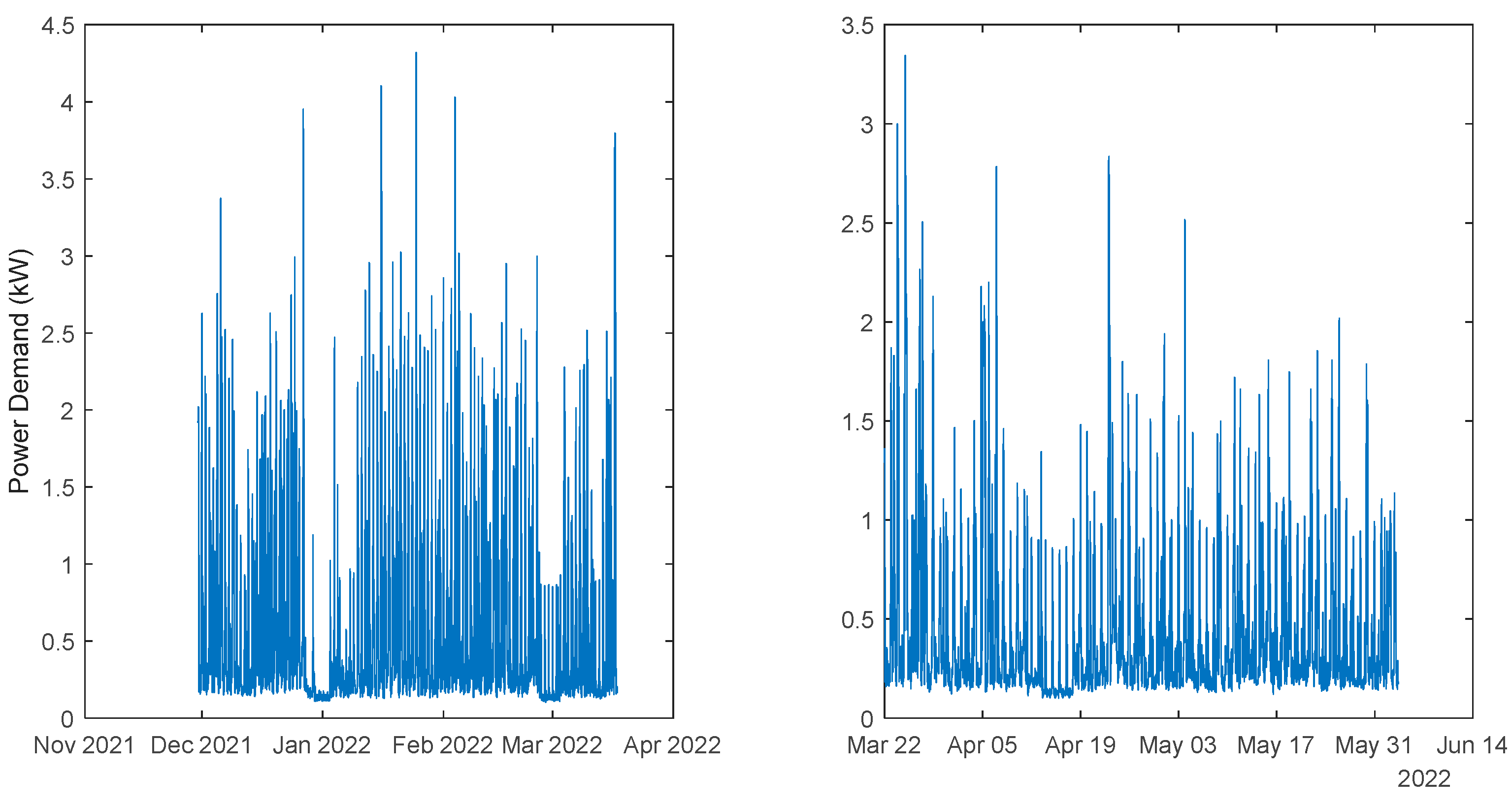
Power Demand: House 3 (triphasic). Left: 1st period; Right: 2nd period.
Figure 6.
Power Demand: House 3 (triphasic). Left: 1st period; Right: 2nd period.
Figure 7.
Power Demand: House 4 (triphasic). Left: 1st period; Right: 2nd period.
Figure 7.
Power Demand: House 4 (triphasic). Left: 1st period; Right: 2nd period.
Figure 8.
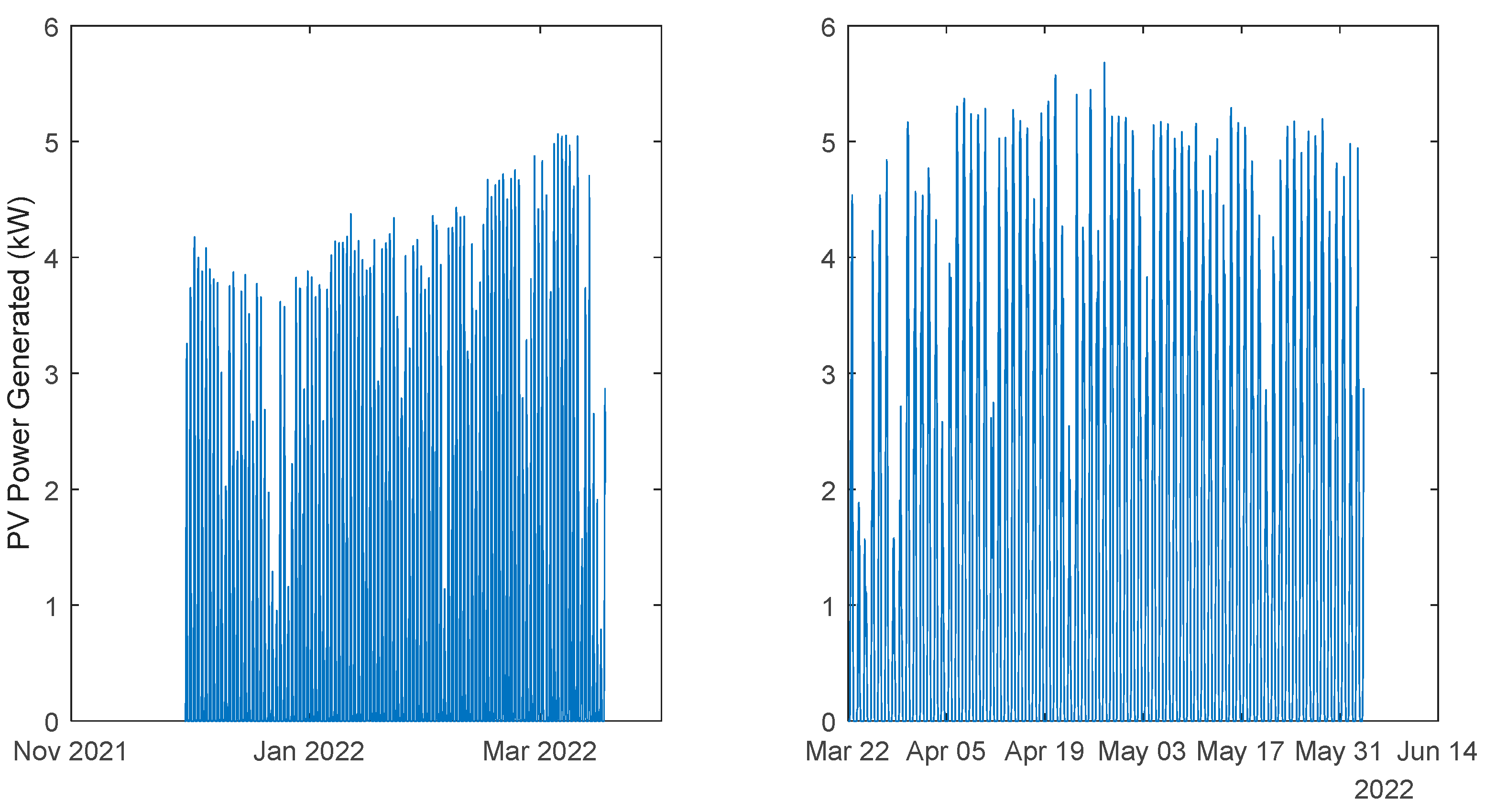
Community Power Generated. Left: 1st period; Right: 2nd period.
Figure 8.
Community Power Generated. Left: 1st period; Right: 2nd period.
Figure 9.
Power delays and forecasts.
Figure 9.
Power delays and forecasts.
Figure 10.
Solar Radiation AW (left) and PINAW (right) forecasts.
Figure 10.
Solar Radiation AW (left) and PINAW (right) forecasts.
Figure 11.
Solar Radiation WS (left) and PINAD (right) forecasts.
Figure 11.
Solar Radiation WS (left) and PINAD (right) forecasts.
Figure 12.
Solar Radiation PICP (left) and RMSE (right) forecasts.
Figure 12.
Solar Radiation PICP (left) and RMSE (right) forecasts.
Figure 13.
Solar Radiation MAE (left) and MAPE (right) forecasts.
Figure 13.
Solar Radiation MAE (left) and MAPE (right) forecasts.
Figure 14.
Solar Radiation R2 forecasts.
Figure 14.
Solar Radiation R2 forecasts.
Figure 15.
Solar Radiation 1-step-ahead. Left: One Day; Right: All days in the prediction time-series. The ‘o’ symbols denote target upper bound violations, and the symbols ‘*’ the lower bound violations by the target. The x-axis label denotes the samples of the prediction time-series.
Figure 15.
Solar Radiation 1-step-ahead. Left: One Day; Right: All days in the prediction time-series. The ‘o’ symbols denote target upper bound violations, and the symbols ‘*’ the lower bound violations by the target. The x-axis label denotes the samples of the prediction time-series.
Figure 16.
Solar Radiation [1, 5, 11, ..., 36]-steps-ahead. The same notation of
Figure 15 right is used.
Figure 16.
Solar Radiation [1, 5, 11, ..., 36]-steps-ahead. The same notation of
Figure 15 right is used.
Figure 17.
Solar Radiation next day forecast computed with data measured up to 12h the day before. The same notation of
Figure 15 right is used.
Figure 17.
Solar Radiation next day forecast computed with data measured up to 12h the day before. The same notation of
Figure 15 right is used.
Figure 18.
Air temperature snapshot.
Figure 18.
Air temperature snapshot.
Figure 19.
Atmospheric Temperature 1-step-ahead. Left: One Day; Right: All days in the prediction time-series.
Figure 19.
Atmospheric Temperature 1-step-ahead. Left: One Day; Right: All days in the prediction time-series.
Figure 20.
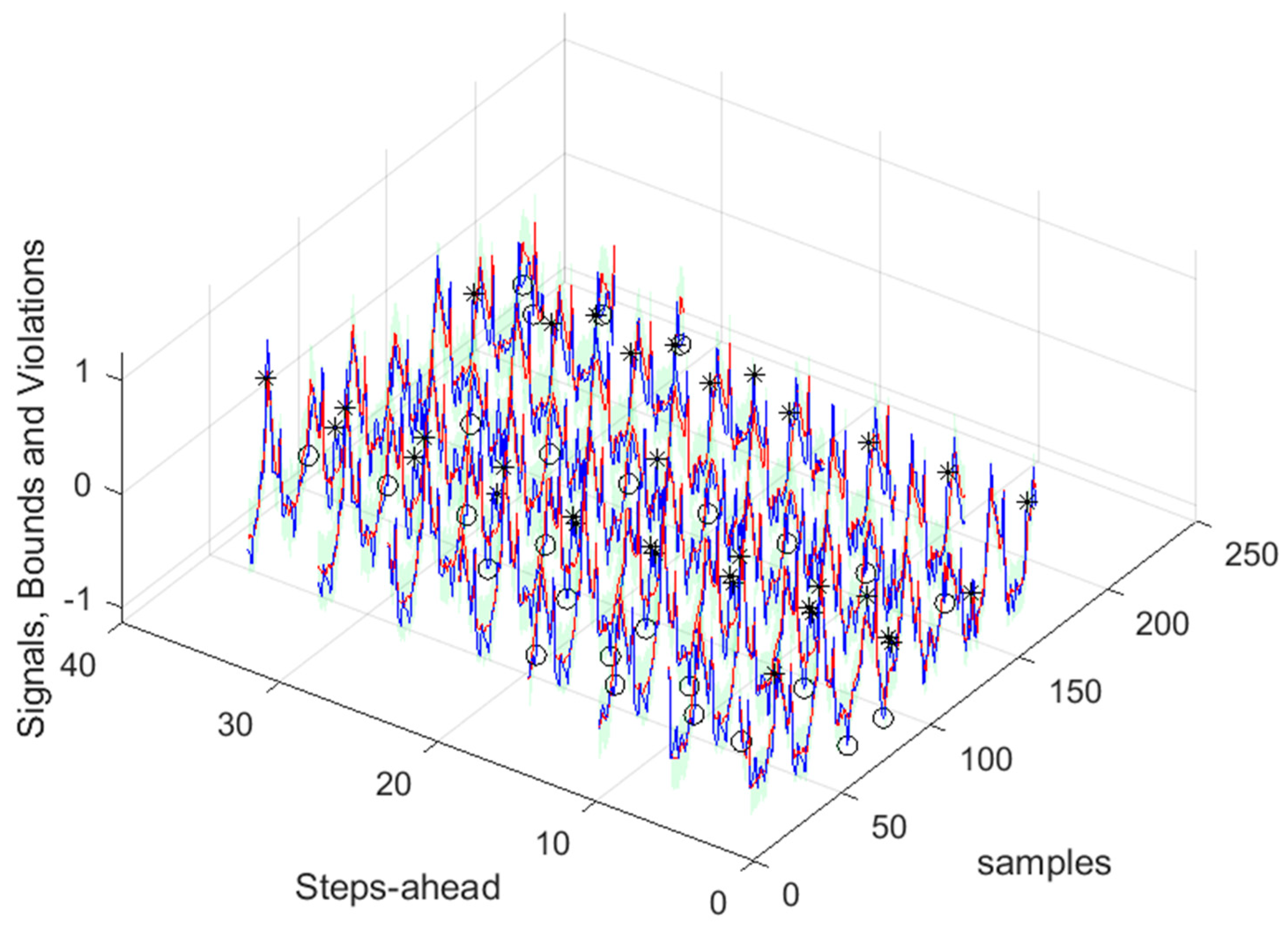
Atmospheric Temperature [1, 5, 11, ..., 36]-steps-ahead.
Figure 20.
Atmospheric Temperature [1, 5, 11, ..., 36]-steps-ahead.
Figure 21.
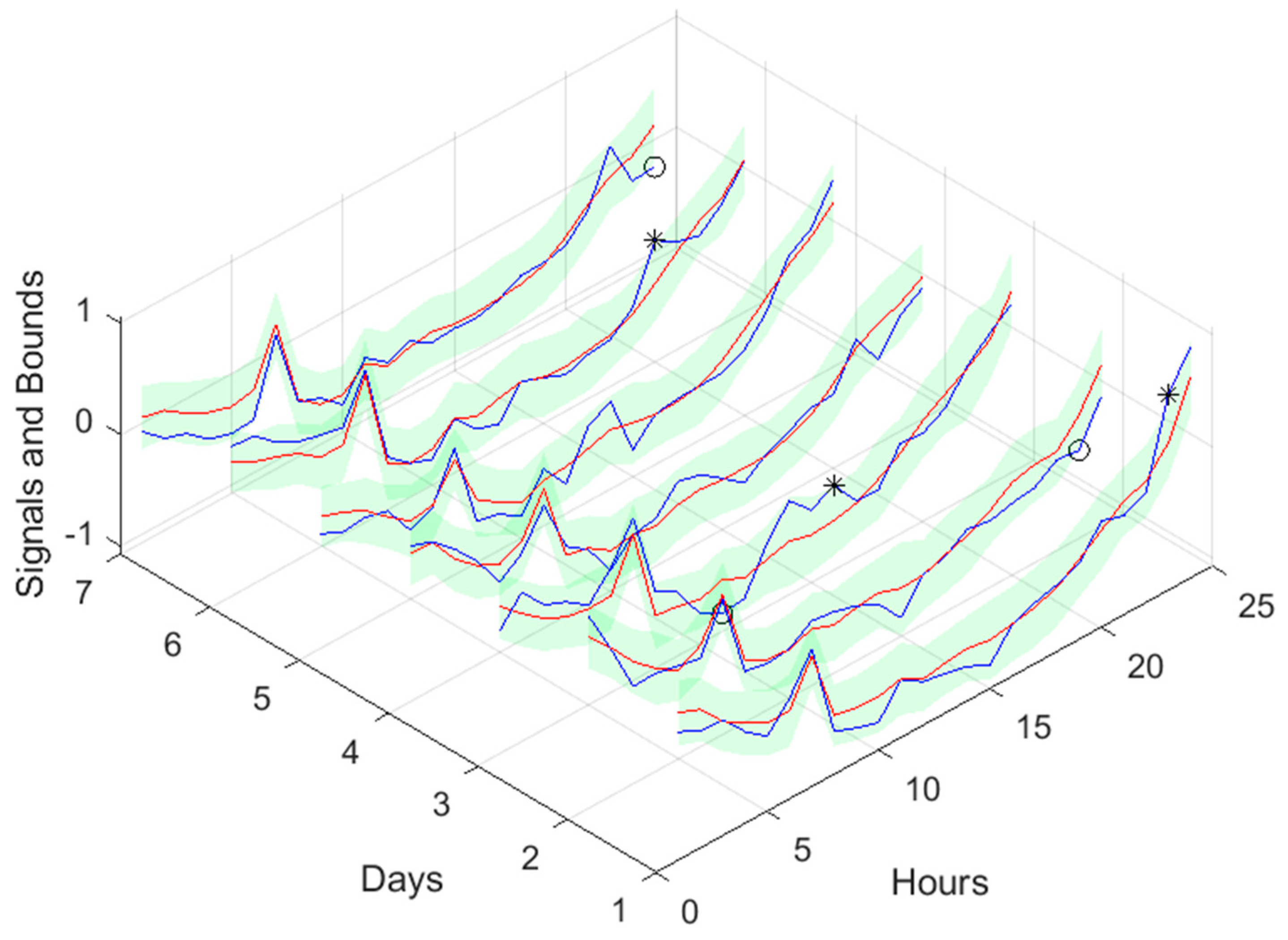
Atmospheric Temperature next day forecast, with measured data until 12h the day before.
Figure 21.
Atmospheric Temperature next day forecast, with measured data until 12h the day before.
Figure 22.
Power Generation 1-step-ahead. Left: One Day; Right: All days in the prediction time-series.
Figure 22.
Power Generation 1-step-ahead. Left: One Day; Right: All days in the prediction time-series.
Figure 23.
Power Generation [1, 5, 11, ..., 36]-steps-ahead.
Figure 23.
Power Generation [1, 5, 11, ..., 36]-steps-ahead.
Figure 24.
Power Generation next day forecast, with measured data until 12h the day before.
Figure 24.
Power Generation next day forecast, with measured data until 12h the day before.
Figure 25.
MP1 Load Demand 1-step-ahead. Left: One Day; Right: All days in the prediction time-series.
Figure 25.
MP1 Load Demand 1-step-ahead. Left: One Day; Right: All days in the prediction time-series.
Figure 26.
MP1 Load Demand [1, 5, 11, ..., 36]-steps-ahead.
Figure 26.
MP1 Load Demand [1, 5, 11, ..., 36]-steps-ahead.
Figure 27.
MP1 Load Demand next day forecast, with measured data until 12h the day before.
Figure 27.
MP1 Load Demand next day forecast, with measured data until 12h the day before.
Figure 28.
MP2 Load Demand 1-step-ahead. Left: One Day; Right: All days in the prediction time-series.
Figure 28.
MP2 Load Demand 1-step-ahead. Left: One Day; Right: All days in the prediction time-series.
Figure 29.
MP2 Load Demand [1, 5, 11, ..., 36]-steps-ahead.
Figure 29.
MP2 Load Demand [1, 5, 11, ..., 36]-steps-ahead.
Figure 30.
MP2 Load Demand next day forecast, with measured data until 12h the day before.
Figure 30.
MP2 Load Demand next day forecast, with measured data until 12h the day before.
Figure 31.
TP1 Load Demand 1-step-ahead. Left: One Day; Right: All days in the prediction time-series.
Figure 31.
TP1 Load Demand 1-step-ahead. Left: One Day; Right: All days in the prediction time-series.
Figure 32.
TP1 Load Demand [1, 5, 11, ..., 36]-steps-ahead.
Figure 32.
TP1 Load Demand [1, 5, 11, ..., 36]-steps-ahead.
Figure 33.
TP1 Load Demand next day forecast, with measured data until 12h the day before.
Figure 33.
TP1 Load Demand next day forecast, with measured data until 12h the day before.
Figure 34.
TP2 Load Demand 1-step-ahead. Left: One Day; Right: All days in the prediction time-series.
Figure 34.
TP2 Load Demand 1-step-ahead. Left: One Day; Right: All days in the prediction time-series.
Figure 35.
TP2 Load Demand [1, 5, 11, ..., 36]-steps-ahead.
Figure 35.
TP2 Load Demand [1, 5, 11, ..., 36]-steps-ahead.
Figure 36.
TP2 Load Demand next day forecast, with measured data until 12h the day before.
Figure 36.
TP2 Load Demand next day forecast, with measured data until 12h the day before.
Figure 37.
Community Load Demand 1-step-ahead. Left: One Day; Right: All days in the prediction time-series.
Figure 37.
Community Load Demand 1-step-ahead. Left: One Day; Right: All days in the prediction time-series.
Figure 38.
Community Load Demand [1, 5, 11, ..., 36]-steps-ahead.
Figure 38.
Community Load Demand [1, 5, 11, ..., 36]-steps-ahead.
Figure 39.
Community Load Demand next day forecast, with measured data until 12h the day before.
Figure 39.
Community Load Demand next day forecast, with measured data until 12h the day before.
Figure 40.
Community Load Demand 1-step-ahead. Left: One Day; Right: All days in the prediction time-series.
Figure 40.
Community Load Demand 1-step-ahead. Left: One Day; Right: All days in the prediction time-series.
Figure 41.
Community Load Demand [1, 5, 11, ..., 36]-steps-ahead.
Figure 41.
Community Load Demand [1, 5, 11, ..., 36]-steps-ahead.
Figure 42.
Community Load Demand next day forecast, with measured data until 12h the day before.
Figure 42.
Community Load Demand next day forecast, with measured data until 12h the day before.
Figure 43.
Community Load Demand, Power Generated and Net Load Demand 1-step ahead forecast.
Figure 43.
Community Load Demand, Power Generated and Net Load Demand 1-step ahead forecast.
Figure 44.
Community Net Demand AW (left) and PINAW (right) evolutions.
Figure 44.
Community Net Demand AW (left) and PINAW (right) evolutions.
Figure 45.
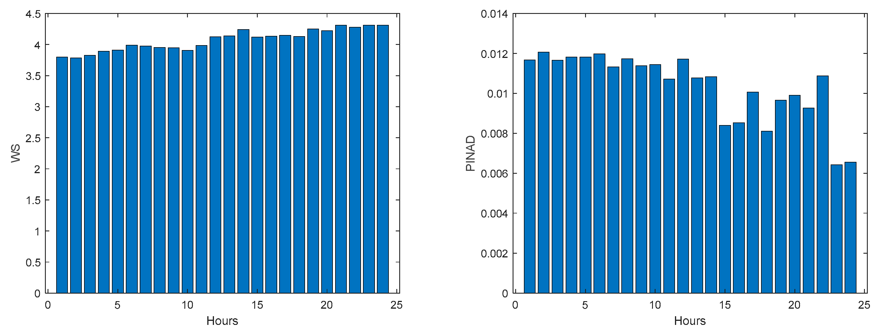
Community Net Demand PINRW (left) and PINAD (right) evolutions.
Figure 45.
Community Net Demand PINRW (left) and PINAD (right) evolutions.
Figure 46.
Community Net Demand PICP (left) and RMSE (right) evolutions.
Figure 46.
Community Net Demand PICP (left) and RMSE (right) evolutions.
Figure 47.
Community Net Demand MAE (left) and MRE (right) evolutions.
Figure 47.
Community Net Demand MAE (left) and MRE (right) evolutions.
Figure 48.
Community Net Demand MAPE (left) and R2 (right) evolutions.
Figure 48.
Community Net Demand MAPE (left) and R2 (right) evolutions.
Figure 49.
Community Net Demand [1, 4, 8, ..., 24] hours in the day-ahead.
Figure 49.
Community Net Demand [1, 4, 8, ..., 24] hours in the day-ahead.
Figure 50.
Community Net Demand next day forecast, with measured data until 12h the day before.
Figure 50.
Community Net Demand next day forecast, with measured data until 12h the day before.
Table 1.
Day encoding.
| Day of the Week |
Regular Day |
Holiday |
Special |
| Monday |
0.05 |
0.40 |
0.70 |
| Tuesday |
0.10 |
0.80 |
|
| Wednesday |
0.15 |
0.50 |
|
| Thursday |
0.20 |
1.00 |
|
| Friday |
0.25 |
0.60 |
0.90 |
| Saturday |
0.30 |
0.30 |
|
| Sunday |
0.35 |
0.35 |
|
Table 2.
Solar Radiation Ensemble Model statistics.
Table 2.
Solar Radiation Ensemble Model statistics.
|
|
|
|
|
|
|
|
|
| 0.30 |
0.26 |
0.73 |
0.02 |
0.92 |
0.08 |
0.04 |
74 |
0.96 |
Table 3.
Atmospheric Air Temperature Ensemble Model statistics.
Table 3.
Atmospheric Air Temperature Ensemble Model statistics.
|
|
|
|
|
|
|
|
|
| 0.42 |
0.41 |
1.21 |
0.04 |
0.91 |
0.12 |
0.08 |
142.36 |
0.77 |
Table 4.
Power Generation Ensemble Model statistics.
Table 4.
Power Generation Ensemble Model statistics.
|
|
|
|
|
|
|
|
|
|
| 0.36 |
0.23 |
0.66 |
0.01 |
0.94 |
0.08 |
0.04 |
2.64 |
54.32 |
0.97 |
Table 5.
Monophasic House 1 Load Demand Ensemble Model statistics.
Table 5.
Monophasic House 1 Load Demand Ensemble Model statistics.
|
|
|
|
|
|
|
|
|
| 1.22 |
0.67 |
1.33 |
0.003 |
0.96 |
0.26 |
0.21 |
233.30 |
0.70 |
Table 6.
Monophasic House 2 Load Demand Ensemble Model statistics.
Table 6.
Monophasic House 2 Load Demand Ensemble Model statistics.
|
|
|
|
|
|
|
|
|
| 0.72 |
0.37 |
1.32 |
0.02 |
0.94 |
0.18 |
0.14 |
140.26 |
0.86 |
Table 7.
Triphasic House 1 Load Demand Ensemble Model statistics.
Table 7.
Triphasic House 1 Load Demand Ensemble Model statistics.
|
|
|
|
|
|
|
|
|
| 0.71 |
0.54 |
1.17 |
0.02 |
0.94 |
0.17 |
0.12 |
150.62 |
0.39 |
Table 8.
Triphasic House 2 Load Demand Ensemble Model statistics.
Table 8.
Triphasic House 2 Load Demand Ensemble Model statistics.
|
|
|
|
|
|
|
|
|
| 0.87 |
0.44 |
0.99 |
0.003 |
0.96 |
0.17 |
0.12 |
99.95 |
0.77 |
Table 9.
Community Load Demand Ensemble Model statistics.
Table 9.
Community Load Demand Ensemble Model statistics.
|
|
|
|
|
|
|
|
|
| 0.87 |
0.44 |
0.99 |
0.003 |
0.96 |
0.15 |
0.11 |
85.01 |
0.84 |
Table 10.
Community Load Demand Ensemble Model statistics.
Table 10.
Community Load Demand Ensemble Model statistics.
|
|
|
|
|
|
|
|
|
| 0.60 |
0.31 |
0.86 |
0.01 |
0.96 |
0.15 |
0.12 |
87.77 |
0.84 |
Table 11.
Net Load Demand Ensemble Model statistics (original scale, 13-36 steps-ahead).
Table 11.
Net Load Demand Ensemble Model statistics (original scale, 13-36 steps-ahead).
|
|
|
|
|
|
|
|
|
| 3.95 |
0.28 |
4.07 |
0.0004 |
0.97 |
0.89 |
0.71 |
473.17 |
0.91 |
