
Submitted:
08 January 2024
Posted:
09 January 2024
You are already at the latest version
Abstract
Vehicular traffic in urban areas continues to be a constant challenge today, due to the continuous population growth and the increase of vehicles in circulation. Vehicular congestion, as a recurrent problem, generates a negative impact on urban mobility and citizens’ quality of life. It is hypothesized that a dynamic clustering method of vehicle trajectory data can provide an accurate and up-to-date representation of real-time traffic behavior. To evaluate this hypothesis, data were collected from three different cities: San Francisco, Rome and Guayaquil. A dynamic clustering algorithm was applied to identify traffic congestion patterns and an indicator was applied to identify and evaluate the congestion conditions of the areas. The results show a high precision and recall in congestion classification compared to a method based on static cells.
Keywords:
congestion
; dynamic clustering
; classification
; GPS trajectories
; road networks
1. Introduction
Examining and analyzing urban vehicular traffic is an extremely important issue in contemporary society. The persistent growth of urban populations and the subsequent rise in vehicular volume create notable impediments to effective traffic management within urban landscapes [1]. This area of management must address crucial aspects, such as environmental impact and road safety, and is fundamental to improving the quality of life of citizens.
Efficient traffic management becomes imperative to improve road flow, reduce travel times and minimize pollutant emissions. It is important to note that traditional approaches may not be agile enough to adapt to variations in traffic conditions, which can be significant throughout the day.
In this environment, the imperative to comprehend the real-time interactions of vehicles and pedestrians in urban landscapes necessitates the comprehensive collection of data from diverse outlets, such as traffic sensors and navigation systems. The utilization of clustering techniques proves indispensable in effectively portraying these data streams, enabling the discernment of traffic patterns, the structuring of data into clusters founded on similarities, and the anticipation of forthcoming trends in urban traffic dynamics. Vital for crafting traffic plans and managing intricacies, these techniques are pivotal in tailoring approaches to meet the distinct demands of individual areas.
Thus, the succeeding research queries come into play: How to identify dynamically patterned traffic areas? How does the use of a clustering algorithm influence the identification of realistic congestion? What is the impact of using a congestion indicator in the process of classifying congested areas? The resolution to these inquiries is reserved for the conclusion of this investigative inquiry.
The focal point in this scenario is the development of a method for identifying and classifying congested areas based on a dynamic clustering algorithm and a congestion indicator. This method will process vehicle trajectory data and road network maps in order to identify and classify congestion zones accurately and efficiently.
This article unfolds in the following manner: Section 2 delves into pertinent literature, dissecting related works and proposing diverse solutions; Section 3 articulates the details of the proposed method; Section 4 showcases the acquired results; Section 5 engages in a discourse on the outcomes; and finally, Section 6 elucidates the conclusions drawn and outlines future avenues of research.
2. Related Work
The exploration of vehicular trajectory data streams in research has been thorough, with numerous studies devising clustering methods tailored to diverse applications [2,3,4]. Through the use of data streams, alternatives have been proposed to improve traffic management by analyzing the spatial structure and extracting traffic-related features [5]. The improvement in efficient traffic management is evidenced by the enriched analysis of data streams when users actively participate, providing feedback that contributes to improve the systems [6].
While there are challenges such as scalability and the volume of data present in the processing that can impact the identification objectives, several researches have proposed alternatives to overcome them, such as techniques that deal with data validation to process more compact data sets without impacting the quality or performance of the processing [7,8,9].
Many of the methods have proven useful in identifying clusters with similarities and analyzing their collective behavior [10], enabling the discernment of patterns and structures within vehicle trajectory data, encompassing the identification of areas prone to congestion.
Previous research has proposed strategies that combine trajectory segmentation [11] with the clustering process in order to obtain higher quality clusters [12,13]. In the field of vehicular trajectory analysis, researchers have frequently adjusted classical clustering algorithms, such as k-means [2] and DBSCAN [14], incorporating similarity metrics tailored to address the intricacies inherent in vehicular trajectories [15,16].
There are identification proposals for static clustering that use, as a basis, a fixed grid-based technique to process data streams from various features [17,18]. Although this processing method leads to the identification of different congestion patterns in a simple way [19], they have the disadvantage that they keep in the background the temporal characteristic present in the data of the trajectories, this disadvantage causes that the information of the clusters can present persistent patterns that should not be present if it is analyzed temporally.
Conversely, emphasizing the need to account for the dynamics of vehicular flow in traffic management, one viable option is to handle trajectory data in brief, periodic flows, allowing for more frequent updates to the clusters [20], this alternative has the disadvantage that these results entail a slight delay to keep the clusters updated for each period, being unfavorable for cases where it is required to show results in real time.
In addition, researchers have delved into the realm of dynamic clustering algorithms to manage the continuous influx of trajectory data and dynamically adjust to shifts in traffic patterns over time. Through the implementation of these dynamic approaches, timely identification of emerging congestion is possible [21,22].
In the most current studies, the combination of machine learning and data mining methodologies has been employed to unearth concealed patterns and anomalies within the dynamics of traffic circulation [23,24,25], as well as to predict vehicle flow in real time. Integrating clustering approaches with diverse analytical methods affords a holistic and systematic perspective on vehicular movement across different scenarios [26,27,28].
In parallel, traffic congestion assessment has established itself as a critical component in the effective management of road networks. Numerous investigations have devised methodologies and approaches for accurately pinpointing congested zones, employing a diverse array of criteria, spanning intricate elements like delay constraints to more straightforward factors such as traffic speeds [23,27,29,30,31]. In addition, machine learning has proven effective in making use of both historical and real-time data to detect recurring congestion and anticipate congestion conditions in real time [32,33].
Due to the continuous increase of information that in certain cases can make it challenging to visualize results, effective and innovative ways to represent traffic congestion trends are being sought [34].
In examining data flows from vehicular trajectories, a dual approach is evident, with a primary focus on both assessing traffic congestion and employing clustering algorithms [35,36,37]. The convergence of these perspectives represents a promising area of research, offering an effective approach to vehicular flow analysis.
A multitude of papers have showcased diverse solutions, including a methodology for examining vehicular flow in defined zones, identifying speed ranges, and upkeeping an interactive map that stays current, aiding in the manual inspection of congestion-prone regions [18]. Although this representation provides a summarized view of real-time traffic, it is essential to incorporate additional information to enrich the analysis of vehicular flow [38], such as information from the road infrastructure or information from different sensors.
The present study introduces an approach for examining vehicular movement, involving the clustering of vehicle trajectory data alongside GPS coordinates. Clusters are used to identify areas with diverse vehicle patterns. The dynamic refreshment of clusters ensures the availability of current data, promoting a realistic approach to the management of vehicular congestion. Furthermore, a traffic congestion metric is applied to assess traffic saturation, presenting a dynamic overview of the traffic status across different geographical areas.
The proposed method offers promising solutions to address the aforementioned challenges, making use of methods such as distance-based clustering and evaluation of a congestion indicator. Distinguished by its capacity to adjust to traffic fluctuations, it guarantees the periodic update of clusters with minimal activity, preventing the buildup of outdated data.
3. Materials and Methods
Figure 1 represents the relationship between the components of the method presented in this study, which is composed of two main components that operate independently: : one dedicated to identifying areas where vehicular traffic has similar characteristics and the other focused on analyzing whether these areas have congestion or not. In addition to the previous components, there are two complementary components for the operation of the method, the first one is in charge of generating preloaded areas to be used for the congestion evaluation and the second one is in charge of the visualization of the results.
3.1. Component 1: Preloaded Area Generator
This component is in charge of generating preloaded areas with dimensions similar to the size of the clusters, in order to reduce the processing cost necessary to analyze different road geometries, in addition, it contains referential information from historical data necessary for the congestion indicator that will be used later. The execution of this component is done a priori to the clustering and classification components, this component only needs to be executed once and the information it generates can be applied to different situations.
First the definition of uniformly distributed points that serve as reference to locate each area is made, then a projection around the point is made, this will be the extension of the area for the road analysis.
A projection is made on the road networks of this area and the identification of all roads is carried out. Subsequently, the geometry of the roads intersecting the defined area is cut out. This process involves the identification of all roads crossing the study area, which often requires the use of high precision geographic information systems (GIS). The trimming ensures that only the relevant roads are considered in the analysis of the specified area.
Once the geometry of the networks is delineated, discrete data streams of historical trajectories are analyzed by reviewing vehicle movement data with GPS devices. The objective is to understand vehicle behavior in each area, identifying relevant information related to roadway capacities.
During the execution of this component, the maximum number of vehicles and the maximum allowed speeds per road are determined, these are essential values to evaluate the capacity of the road infrastructure in each area. The generated data are efficiently stored in memory and can be saved in specialized database management systems to ensure integrity and availability for future experiments.
This data generated from preloaded areas contributes to improve the performance of the method as it is a resource that is generated prior to clustering and does not require updating during the processing of new data streams.
Algorithm 1 summarizes the process described above.
| Algorithm 1 Preloaded area generator component. |
|
Input: : list of road networks; : list of historical GPS points; : maximum number of X-axis centers; : maximum number of Y-axis centers; : maximum number of historical instants to be captured
Output: : list of precharged areas
|
3.2. Component 2: Dynamic Point Clustering Algorithm
To process in real time a steady stream of GPS trajectories in this study, an agile and efficient data processing process was implemented.
For this work, a steady stream was simulated and processed by a spatial clustering method to group trajectories with similar motion characteristics. This method allows to efficiently process the steady flow of GPS trajectories and use the resulting information for analysis.
3.2.1. Cluster Formation
A cluster consists of a set of GPS points represented by an average centroid or location. The coverage area of the cluster will be determined by an area called a hyperbox. The centroid is characterized as the geographical reference point that serves as the central representation within the cluster’s set of points. Utilized as a representative focal point for the cluster, this central marker eases the comprehension and analysis of the spatial arrangement. The hyperbox is characterized as a rectangular geometric structure in a two-dimensional space. Its position in space is determined by the centroid of the cluster to which it is associated; the center of the hyperbox coincides with the centroid of the cluster. The incorporation of this rectangular model offers a method to demarcate a region centered on the centroid, streamlining the spatial depiction of the cluster in the analysis while specifying its sphere of influence within the examination.
In Figure 2, a visual illustration showcases the composition of a cluster, providing a graphical overview of its elements.
Each GPS point extracted from the flow is processed individually and contains information on geographic coordinates (latitude and longitude), vehicle identifier and time of entry. Executing the clustering task involves applying a similarity criterion centered on Euclidean distance, harnessing the geographical coordinates of latitude and longitude from the processed data.
Analysis is conducted on every GPS point, computing the Euclidean distance from the point to the centroids of all currently established clusters. Identification is made of the cluster exhibiting the minimal spatial separation between the examined point and its centroid. If the coordinate of the analyzed GPS point coincides within the hyperbox area of the selected cluster, the point is affiliated with the cluster and will be considered an integral part of the cluster. With the incorporation of new GPS points into a given cluster, the centroid undergoes an update to reflect the evolving spatial center of the cluster. During this process, the clusters that receive new points will be updated and in scenarios devoid of proximate clusters, the system generates new clusters.
If the point is not situated within the hyperbox area, a fresh cluster comes into existence Once a point forms an association with a specific cluster, any reassignment to another cluster is precluded.
Within Figure 3, the central details comprising a cluster’s content are depicted.
3.2.2. Percentage of data forgotten
To ensure that the system is up to date and does not retain data that is too old, a forgetting mechanism is introduced, utilizing a percentage approach tied to the entry time of the most recent point.
This forgetting mechanism indicates the percentage of data relevance for each unit of time in seconds elapsed, using Equation 1 to determine this percentage.
where, e corresponds to a function of exponential nature, (lambda) is the parameter that regulates the pace at which the decay unfolds. The decay unfolds more rapidly as attains higher values. Lastly, represents the time gap in seconds between the timestamp of the analyzed point and that of the most recent point assimilated into the cluster.
Each cluster has a numerical indicator that reflects the number of points to remember, this indicator first decreases by a percentage calculated by the forgetting mechanism from each second of time that has elapsed since the last point entered the cluster and then increases by 1 in case a new GPS point is added.
Establishing a 5% tolerance threshold linked to the most effective lambda parameter setting facilitate the choice of this parameter in terms of elapsed time, this threshold has been established from simulations that determine approximately how much percentage of data should be considered according to the time you want to keep data.
This forgetting mechanism is used to filter data or results, focusing attention on those that exceed the tolerance threshold and discarding those that do not. By applying a 5% tolerance cap, we seek to ensure that only values that have a significant degree of importance are remembered in the cluster analysis.
Within the clustering procedure, this mechanism defines the count of GPS points that will endure within the cluster. This will ensure that the system adapts to changes in traffic and avoids accumulation of obsolete data. Those clusters whose GPS points have lost importance due to not receiving a sufficient amount of new GPS points are removed in order to maintain an up-to-date analysis of the traffic situation. At the same time, those active clusters that continue to receive new GPS points will be kept up to date for proper traffic analysis.
A visual representation of the percentage of forgetting and relevance that is considered during the forgetting mechanism is shown in Figure 4, it can be seen that with a time difference of zero seconds the relevance is 100%, and as the elapsed time difference in seconds increases, the percentage of relevance decreases.
The area with the relevant percentage is marked with a green background, and when the percentage falls below the tolerance threshold set at 5%, it is considered not relevant, this area is marked with a red background.
The percentage forgetting mechanism is applied each time a point is added to a cluster. Additionally the forgetting mechanism is applied periodically to clusters that have not received recent points, in order to ensure that these particular clusters are kept up to date.
Algorithm 2 summarizes the process of component 2.
| Algorithm 2 Dynamic point clustering component. |
|
Input: S: data stream; : initial data capture time; : final data capture time; : lambda value
Output: : list of snapshots, : clustering status
|
3.3. Component 3: Cluster Classifier
Through the execution of this component, it becomes possible to individually examine and categorize each cluster based on its congestion level, assisting in the recognition of problematic regions and those displaying improved traffic circulation. While the clustering of the data is performed in real time, a parallel process is used to capture the results of the clustering periodically, using an "Observer".
3.3.1. Observer
The observer assumes a vital function in the recurrent oversight and categorization of the clusters based on their conditions, it is responsible for taking periodic snapshots of the state of the clusters at regular intervals.
The incorporation of the Observer ensures that the information about the state of the clusters that was captured by the snapshots is the most recent and that the classification is based on recent data. This plays a pivotal role in ensuring result accuracy and a thorough comprehension of how traffic congestion evolves across the study areas as time progresses.
At each capture, the Observer records relevant variables describing the status of the clusters. This includes information such as geographic location, number of vehicles present in the area, average speed, and other data related to traffic congestion.
Each snapshot capture is stored in memory, thus minimizing the waiting times required to store each snapshot without affecting the clustering process and avoiding to a large extent the loss of GPS points in the flow. This storage is essential for analyzing trends over time and detecting patterns in traffic congestion.
After each capture, the Observer runs the process of classifying the clusters into congested and non-congested categories. The classification of the clusters is kept up to date with each new capture, thus providing a dynamic view of traffic congestion. This periodic update makes it possible to detect changes over time and analyze how congestion varies according to different conditions and events.
3.3.2. Classification
In this component, the classification of the clusters is carried out in two main categories: those that were congested and those that were not. Unlike the clustering component, the classification is not performed in real time, it is related to the frequency in which the snapshots are generated, so this parameter has a direct impact and can cause additional waiting times if it is set to low frequency values, this factor must be taken into account if you want to show results very close to real time.
The process of analyzing each snapshot involves the iterative execution of each cluster of processes described below:
First, we proceed to the identification of the closest preloaded area, with a precise focus on determining which preloaded area has the greatest similarity with respect to the area that is covered by the cluster being analyzed. Achieving this involves computing the Euclidean distance between the preloaded areas’ centers and the centroids associated with the scrutinized clusters. This metric provides an objective measure of the proximity of each cluster to the preloaded areas, ensuring that the choice of the closest preloaded area determines the reference conditions to be used for the cluster congestion analysis.
Once the nearest preloaded area is identified, detailed information about the road networks present in that area is retrieved. This includes data on the topology of the roads, their maximum capacity, maximum allowable speed and other relevant attributes that facilitate an analysis of the road infrastructure in the area.
Subsequently, the points that make up each cluster are analyzed and these points are assigned to the road segments closest to each point. This process makes it possible to clearly establish to which road network each point in the cluster is associated, which in turn simplifies subsequent analyses.
With the assignment of points completed, average densities and speeds are calculated for each road segment. This provides a quantitative description of roadway operation and allows the identification of segments with a higher vehicular flow and, therefore, a higher probability of congestion.
Density and speed indices are then calculated from the average density and speed data for each road segment. These indices serve as key indicators to assess the state of congestion in the areas of interest.
The classification of the clusters is done based on the values obtained in the TCC, which allows for a detailed characterization of traffic congestion in each area.
3.3.3. Calculation of the Traffic Congestion Coeficient (TCC)
The Traffic Congestion Coefficient (TCC) is an indicator used to measure the level of traffic congestion or saturation in a given area or roadway. The TCC provides a quantitative measure of traffic saturation that reflects how much traffic flow is affected at a given location as a function of vehicle density and speeds. A higher TCC value correlates with increased congestion, whereas a lower TCC value is indicative of reduced congestion and a more seamless traffic flow. To compute this indicator on a road segment, it is essential to account for the potential overlap of a cluster’s hyperbox with multiple segments. Initially, the TCC indicator is individually calculated for each segment, and a cohesive value, determined as a percentage based on the length of segments with at least one registered vehicle, results in a distinctive TCC value for each cluster. The TCC is calculated by the relationship between two indexes as shown in Equation 2.
where, serves as an indicator of area density, while functions as an indicator of the area velocity of the analyzed region.
3.3.4. Density Index
This metric serves as a numerical representation of the vehicular count observed on a designated road segment or within a specified area over a defined time interval. This numerical indicator is computed by dividing the observed vehicle count within the analyzed region by the highest number of vehicles recorded at the same location. The formula for the Density Index is shown in Equation 3.
where, d indicates number of vehicles per length of traveled route and indicates the maximum vehicle density recorded historically.
Established through historical records or thorough traffic assessments specific to the region, this upper threshold for density plays a pivotal role in understanding and analyzing traffic patterns. For this work the value of the maximum density of each road segment is obtained in the component that generates the areas preloaded with this information from historical data. The traffic density index of the different roads in the cluster is then calculated.
The maximum capacity may vary according to the size of the road and other relevant factors. In instances where the Density Index approximates 1 or reaches 1, it denotes that the quantity of vehicles on the studied thoroughfare is approaching or surpassing the maximum capacity observed, suggesting a significant likelihood of traffic congestion. That is, the greater the number of vehicles relative to maximum capacity, the higher the density index and, therefore, the greater the congestion.
3.3.5. Speed Index
This metric denotes the mean velocity of vehicles traversing the surveyed roadways. Quantifying the mean velocity of all trajectories in the examined section or region, this index provides a measure of vehicle movement. It is determined by taking the average vehicle velocities and dividing it by the maximum speed allowed according to the regulations in the given city or area. The maximum allowable speed is usually defined by traffic laws and regulations to ensure road safety and proper traffic flow. The formula for the Speed Index is presented in Equation 4.
where, v indicates average speed of the recorded vehicles and indicates maximum allowable speed on the road on which the vehicle traveled.
If this metric approaches, equals or exceeds the value of 1, it indicates that vehicles are operating at the velocity at which significant traffic congestion is unlikely to occur. If the average speed is low, the speed index will be lower, indicating higher congestion and slower traffic.
Algorithm 3 summarizes the process of component 3. The algorithm concludes its operation based on the execution state of component 2 and the presence of snapshots ready for processing.
| Algorithm 3 Cluster classifier component. |
|
Input: : list of snapshots, : clustering status; : list of precharged areas
Output: : list of snapshots
|
3.4. Component 4: Results viewer
This study involves the periodic analysis of trajectory data, enabling the precise identification of fluctuations in vehicular traffic.
An interactive map has been devised to dynamically present the outputs of each clustering process. This map is generated using snapshots created during clustering or can be examined utilizing the congestion indicator. Through this map, one can conduct real-time graphical scrutiny of pertinent details within each cluster. Distinct colors on the map delineate areas sharing similar traits, as depicted in the illustration found in Figure 5.
Algorithm 4 summarizes the process of component 4.
| Algorithm 4 Results viewer component |
|
Input: : list of snapshots
Output: : snapshot maps
|
4. Results
4.1. Used Data
4.1.1. San Francisco Dataset
The data set for the city of San Francisco was collected on June 02, 2008; it contains 290 trajectories recorded by cabs using GPS devices. Each record contains the following data: trajectory id, latitude, longitude, time, speed and direction. For this set of trajectories, the analysis included all the trajectories recorded between 12:30 p.m. and 13:30 p.m. As a result of this filtering process, 2382 records were obtained, representing 290 trajectories from the entire data set.
These trajectories have been reconstructed by applying a routing and interpolation method every 5 meters from which a total of 182559 points have been obtained.
4.1.2. Rome Dataset
The data set for the city of Rome was collected on February 12, 2014 and contains 137 trajectories performed by cabs collected by GPS devices with an average time interval of 10 seconds between consecutive points. Each record contains trajectory id, latitude, longitude, time, speed, direction.
For this second set of trajectories, the analysis was performed between 18:00 and 19:00 hs. As a result of this filtering process, 33793 records were obtained, representing 137 trajectories of the entire data set.
These trajectories have been reconstructed by applying a routing and interpolation method every 5 meters from which a total of 7790 points have been obtained.
4.1.3. Guayaquil Dataset
This dataset was collected on October 28, 2017 and corresponds to 218 trajectories performed by university students traveling by some means of transportation such as cab, motorcycle, metro-via. The GPS points in this dataset were collected by smartphones with an average time interval of 5 seconds between consecutive points. Each record contains id, latitude, longitude, time, user name, email and type of transportation.
Given that this is a small set of trajectories, the analysis was carried out between 16:30 and 18:30 hrs as it was considered to be the time with the highest concentration of records. As a result of this filtering process, 30557 records were obtained, representing 206 trajectories of the entire data set.
These trajectories have been reconstructed by applying a routing and interpolation method every 5 meters from which a total of 135237 points have been obtained.
4.2. Model Parameter Selection
Within this study, a two-dimensional space has been defined for analysis, spanning an area of 1200 × 800 square meters. Hyperboxes, each with a consistent size of around 35 × 25 meters, were employed, collectively representing approximately 3% of the designated area. The capture and analysis of intantaneas is performed at a frequency of 1 minute each. The similarity measure used is the Euclidean distance, and the lambda parameter () was set to 0.068, which means that the GPS points of the clusters are considered relevant until 45 seconds, GPS points that exceed that time are considered not relevant and are eliminated. Updating at 30-second intervals, clusters characterized by low activity are maintained, while those clusters lacking GPS points for a duration of at least 2 minutes are removed from the system.
4.3. Comparison Method
In this study, two methods for analyzing vehicular flow were compared: dynamic clusters and a static grid, using the TCC to classify congestion.
In the dynamic clustering method, data from vehicle trajectories with similar patterns were grouped and evaluated to determine congestion based on speed and number of vehicles. Employing the static grid method, we partitioned the study area into uniform cells, each characterized by speed and vehicle count information, assessed in accordance with the TCC.
For the dynamic clusters, the cluster hyperbox was projected, as seen in Figure 6 and the TCC values of the overlapping cells were adjusted, considering a tolerance derived from the inherent variability observed in traffic data.
Introducing a tolerance factor offers the flexibility needed to correct potential TCC values influenced by the inherent variability of the data, thereby preventing the misclassification of congestion or non-congestion situations.
This adjustment increases the matching matches in the comparison. For congested clusters, the TCC tolerance of the cells is added, and for non-congested, it is subtracted.
An assessment is carried out, comparing the congested and non-congested states within cells and clusters. Recorded are matches deemed valid when, at a minimum, one cell aligns its classification with that of the cluster.
4.4. Validation of the Model
An initial experiment was undertaken to showcase the dynamic method’s superiority over its static counterpart, illustrating its distinct advantages. The objective of this experiment was to analyze how each method handles the evolving characteristics of traffic information and the circulation of vehicles within a road system. The analysis was conducted to identify specific situations where one method outperforms the other. The experiment is poised to furnish precise data, facilitating a comprehension of variances, and underscoring the superiority of the dynamic approach outlined in this study.
To carry out this experiment, we worked with a representative data set of the city of San Francisco that contemplates 6 minutes of execution, capturing snapshots every one minute in an area of 100 × 100 meters. Randomly chosen from the experiment’s data cluster, a group underwent a detailed comparative analysis. Special focus was placed on the characteristics of the proposed dynamic method, highlighting how it adapts to variations in data distribution over time. These results were compared with a static method based on a fixed grid, highlighting notable differences in its responsiveness to changing traffic conditions and data distribution.
In the proposed dynamic method, the ability to adapt to changing conditions of the spatial distribution of data is a crucial feature. Figure 7 illustrates the adaptive and precise adjustments of the centroid and hyperbox location at various time instances, ensuring coverage along road segments and adeptly capturing changes in both cluster density and shape. This update not only reflects the current distribution of the data, but also allows the model to adjust for possible deviations and changes in the shape of the clusters over time.
A representation of the dynamism over a cluster over four consecutive seconds of processing GPS points is shown in Figure 7, the new points that are integrated into the cluster update the centroid and hyperbox causing a slight displacement of both according to the coordinates of the new GPS points. It can also be identified that the oldest GPS points lose relevance as time goes by (in the graph they are marked in red) and are the ones that will eventually be removed from the cluster in future instants (marked with red edges).
In this method the data are processed in time order, which is important to distinguish old points and to keep the cluster location updated, the points processed for each time instant in the clustering can be visualized in Figure 8. A representation of the hyperbox of the analyzed cluster has been projected to identify the points that have been assigned to this particular cluster, moreover, as the points can only be assigned to a single cluster, the other points that are displayed and are outside the projected hyperbox are assigned to some other cluster than the analyzed one. The points displayed with black color correspond to points that entered at one time instant, while the points with red borders are points that entered at the previous time instant.
On the other hand, the static method, which is based on a fixed grid, has certain limitations in terms of adaptability. In Figure 9 it can be seen how the data are assigned to predefined cells in the grid. GPS points transiting a road are assigned and analyzed as part of a cell and this cell serves a certain specific region, therefore, several cells are required to analyze a large road and GPS points will be distributed among the different cells. The distribution of cells in a fixed grid ensures complete coverage allowing an understanding of the spatial dynamics of roads in their respective areas and the consideration of how GPS points are distributed between cells suggests attention to efficiency in spatial data management. But, in a fixed grid the need to use several cells to analyze a road that traverses multiple areas also presents its own disadvantages, for example, the road may appear to be divided which may affect the understanding of its whole, this management of cells may require more computational and storage resources, in addition, some risks of errors may occur when coordinating data between cells.
As for the dynamism of the data when analyzing the snapshots using the classifier component, the dynamic method shows a clear advantage. In the Figure 10 shows the selection of road segments for the snapshots captured at minutes 1 (Figure 10a), 3 (Figure 10b) and 5 (Figure 10c) used for congestion assessment, this capacity to flexibly adapt to shifts in data location and make adjustments to centroids and hyperboxes as required positions it as an excellent option for identifying segments affected by changes in vehicular flow and traffic density. On the other hand, the static method grapples with managing these dynamics, as the rigid lattice fails to adjust effectively to fluctuations.
In real scenarios, such as a road network traversing an urban area with multiple routes and traffic patterns, diverse situations arise. During peak traffic hours, roads can fill up with a large number of vehicles, resulting in congestion. In contrast, during off-peak times, the number of vehicles on the roads decreases. If we focus on a static method that does not consider these fluctuations in data flows, as can be seen in Figure 11 the road segments being analyzed remain fixed at all times, there is a possibility that roads with very different traffic volumes will be incorrectly selected for each cell. This erroneous choice may result in an imprecise portrayal of how vehicles behave throughout various periods within the day.
During this initial experiment, a salient feature of the dynamic approach can be observed, in contrast to the static alternative that computes the congestion indicator using all observed points but without considering the evolution of the vehicle route. , the static method only retains the recent points considered relevant to the vehicles, as these are the ones that approximate a real time route of the vehicles.
Within the dynamic approach, as vehicles navigate and fresh GPS data is logged, the clustering algorithm assimilates these GPS points into their designated clusters, thereby triggering an autonomous update of the centroid. This suggests that the definition of real-time congestion is more significantly influenced by the most recent GPS points, while the relevance of earlier GPS data gradually diminishes.
This differentiation is crucial, since in one trip, a vehicle may cross multiple cells and its trajectory may span a variety of GPS points. If all these GPS points were considered without taking into account temporal dynamics, erroneous conclusions about congestion could be reached, identifying congestion that does not actually exist. Consequently, the dynamic method secures a real-time assessment of congestion that is both precise and adaptable, effectively responding to the dynamic nature of vehicle mobility on urban roadways.
4.5. Obtained Results
In order to measure the effectiveness of this method, a table has been generated with the execution times. This table provides a detailed and objective view of how the method behaves in practical conditions.
In the parallel execution process, it is relevant to note that the times of the clustering component are measured independently, while the classification and visualization components are evaluated together and separately to the classification component, the results of the execution times are shown in Table 1 for 60-second snapshots and in Table 2 for 30-second snapshots both in unit of measure in minute and are obtained from running one hour of data in the cities of San Francisco, Rome and Guayaquil. This individualized measurement strategy allows a more precise analysis of each component and its contribution to the total run time. In addition, in parallel executions it is common to observe that the maximum time of the processes to be measured is taken as a reference.
The results show significant differences in the execution times of the clustering and classification components in the cities of San Francisco, Rome and Guayaquil. Although areas of very similar dimensions were used, there are several reasons that may explain these disparities.
In the case of the clustering component, the experiments with 60-second snapshots showed that the city of San Francisco shows the longest time, at 28 minutes and 23 seconds. This could be due to the complexity of the data in that city or a larger amount of data requiring processing. On the other hand, Rome and Guayaquil show shorter times, 10 minutes and 46 seconds and 18 minutes and 32 seconds, respectively.
Experiments with 30-second snapshots showed that the city of San Francisco requires 27 minutes and 34 seconds for clustering, while the city of Rome requires 11 minutes and 2 seconds, and the city of Guayaquil requires 18 minutes and 37 seconds.
This could indicate a higher efficiency in the clustering process in those cities or a lower workload that could be directly related to the number of trajectories. In the experiments with 60-second snapshots, San Francisco was processed with 290 trajectories and has obtained the longest processing time, Guayaquil with 218 trajectories has obtained a shorter time than San Francisco, and finally Rome obtained the shortest processing time by processing 137 trajectories, this trend is also present in the 30-second experiments which reaffirms that there is a direct relationship between processing time and the amount of clustered trajectories.
The storage of each snapshot takes less than 0.02 seconds, during this time the clustering stops momentarily, however, this time is relatively small which does not affect the clustering processing time since if compared to the time between snapshots which is 60 seconds, this time represents 0.03%.
As for the classification component, the experiments performed with 60-second snapshots show that the Guayaquil dataset stands out with the lowest time, 7 minutes and 40 seconds, followed by Rome with 8 minutes and 30 seconds. San Francisco, in this case, shows the longest time, 19 minutes and 11 seconds. For the experiments with 30-second snapshots, the order is preserved with respect to the time required to classify each cluster, obtaining 39 minutes and 1 second in the city of San Francisco, 31 minutes and 41 seconds in the city of Guayaquil, and 15 minutes and 13 seconds for the city of Rome. These times could be related to the availability of processing resources in each location or the complexity of the road networks found in the areas used for classification in each city.
The variability in the layout of the available roads in a city can directly influence the performance of the system, some examples are given to illustrate some cases faced by the cluster classification component, Figure 12a shows the simplest case that will require the least amount of resources to analyze, the case of Figure 12b is a scenario with a very common urban distribution between cities that will require more time to obtain the traffic valuation, and Figure 12c shows the case of a complex road network that is composed of multiple intersecting roads.
From the perspective of parallel execution, these results highlight the importance of considering the performance of each component separately. Parallel execution allows the workload to be distributed efficiently, but execution times vary depending on the processing power of each component and how they interact with each other.
To verify the precision of the clustering classification, an evaluation is applied based on the observed results, which are reflected in different confusion matrices for each city evaluated. The confusion matrix delivers a compact portrayal of the classification model’s effectiveness in gauging TCC grid congestion. It quantifies the instances of correct and incorrect predictions within the respective TCC categories.
Table 3 exhibits the findings of the confusion matrixes using from 60-second snapshots for the San Francisco dataset. For a tolerance of 0.2, the matrix reveals that the model was able to correctly identify 11237 cases of congestion and 2503 cases of non-congestion. However, in the cases of incorrect classifications, there are 166 cases in which scenarios without congestion are identified when the static method indicates that they are congested scenarios, while in the other category there are 1748 cases in which congested scenarios are identified, but the static method indicates that these scenarios are not congested.
For a tolerance of 0.1, the matrix reveals that the model was able to correctly identify 10614 cases of congestion and 2492 cases of non-congestion. However, in the cases of incorrect classifications, there are 176 cases in which scenarios without congestion are identified when the static method indicates that they are congested scenarios, while in the other category there are 2371 cases in which congested scenarios are identified, but the static method indicates that these scenarios are not congested.
For a tolerance of 0, the matrix reveals that the model was able to correctly identify 10029 cases of congestion and 2457 cases of non-congestion. However, in the cases of incorrect classifications, there are 211 cases in which scenarios without congestion are identified when the static method indicates that they are congested scenarios, while in the other category there are 2956 cases in which congested scenarios are identified, but the static method indicates that these scenarios are not congested.
Table 4 exhibits the findings of the confusion matrixes using from 30-second snapshots for the San Francisco dataset. For a tolerance of 0.2, the matrix reveals that the model was able to correctly identify 14184 cases of congestion and 3294 cases of non-congestion. However, in the cases of incorrect classifications, there are 1227 cases in which scenarios without congestion are identified when the static method indicates that they are congested scenarios, while in the other category there are 7062 cases in which congested scenarios are identified, but the static method indicates that these scenarios are not congested.
For a tolerance of 0.1, the matrix reveals that the model was able to correctly identify 13335 cases of congestion and 3258 cases of non-congestion. However, in the cases of incorrect classifications, there are 1263 cases in which scenarios without congestion are identified when the static method indicates that they are congested scenarios, while in the other category there are 7911 cases in which congested scenarios are identified, but the static method indicates that these scenarios are not congested.
For a tolerance of 0, the matrix reveals that the model was able to correctly identify 12471 cases of congestion and 3234 cases of non-congestion. However, in the cases of incorrect classifications, there are 1287 cases in which scenarios without congestion are identified when the static method indicates that they are congested scenarios, while in the other category there are 8775 cases in which congested scenarios are identified, but the static method indicates that these scenarios are not congested.
The results of the confusion matrixes for the city of Rome using 60-second snapshots are shown in Table 5. Specifically for a tolerance of 0.2, the model was able to get 3195 cases of congestion and 412 cases of non-congestion correct. However, in the cases of incorrect classifications, there are 30 cases in which scenarios without congestion are identified when the static method indicates that they are congested scenarios, while in the other category there are 309 cases in which congested scenarios are identified, but the static method indicates that these scenarios are not congested.
For a tolerance of 0.1, the matrix reveals that the model was able to correctly identify 3089 congested cases and 412 non-congested cases. However, in the cases of incorrect classifications, there are 30 cases in which scenarios without congestion are identified when the static method indicates that they are congested scenarios, while in the other category there are 415 cases in which congested scenarios are identified, but the static method indicates that these scenarios are not congested.
For a tolerance of 0, the matrix reveals that the model was able to correctly identify 2994 cases of congestion and 408 cases of non-congestion. However, in the cases of incorrect classifications, there are 34 cases in which scenarios without congestion are identified when the static method indicates that they are congested scenarios, while in the other category there are 510 cases in which congested scenarios are identified, but the static method indicates that these scenarios are not congested.
The results of the confusion matrixes for the city of Rome using 30-second snapshots are shown in Table 6. Specifically for a tolerance of 0.2, the model was able to hit 4689 cases of congestion and 509 cases of non-congestion. However, in the cases of incorrect classifications, there are 390 cases in which scenarios without congestion are identified when the static method indicates that they are congested scenarios, while in the other category there are 2159 cases in which congested scenarios are identified, but the static method indicates that these scenarios are not congested.
For a tolerance of 0.1, the matrix reveals that the model was able to correctly identify 4594 congested cases and 508 non-congested cases. However, in the cases of incorrect classifications, there are 391 cases in which scenarios without congestion are identified when the static method indicates that they are congested scenarios, while in the other category there are 2254 cases in which congested scenarios are identified, but the static method indicates that these scenarios are not congested.
For a tolerance of 0, the matrix reveals that the model was able to correctly identify 4497 cases of congestion and 500 cases of non-congestion. However, in the cases of incorrect classifications, there are 399 cases in which scenarios without congestion are identified when the static method indicates that they are congested scenarios, while in the other category there are 2351 cases in which congested scenarios are identified, but the static method indicates that these scenarios are not congested.
The results of the confusion matrixes for the city of Guayaquil, using 60-second snapshots, are shown in Table 7. In particular, for a tolerance of 0.2, the model was successful in 2576 congestion situations and 1912 cases of no congestion. However, in the cases of incorrect classifications, there are 146 cases in which scenarios without congestion are identified when the static method indicates that they are congested scenarios, while in the other category there are 276 cases in which congested scenarios are identified, but the static method indicates that these scenarios are not congested.
For a tolerance of 0.1, the matrix reveals that the model was able to correctly identify 2535 congested cases and 1891 non-congested cases. However, in the cases of incorrect classifications, there are 167 cases in which scenarios without congestion are identified when the static method indicates that they are congested scenarios, while in the other category there are 317 cases in which congested scenarios are identified, but the static method indicates that these scenarios are not congested.
For a tolerance of 0, the matrix reveals that the model was able to correctly identify 2459 cases of congestion and 1872 cases of non-congestion. However, in the cases of incorrect classifications, there are 186 cases in which scenarios without congestion are identified when the static method indicates that they are congested scenarios, while in the other category there are 393 cases in which congested scenarios are identified, but the static method indicates that these scenarios are not congested.
The results of the confusion matrixes for the city of Guayaquil, using 60-second snapshots, are shown in Table 8. In particular, for a tolerance of 0.2, the model was successful in 3364 congestion situations and 2328 cases of no congestion. However, in the cases of incorrect classifications, there are 1193 cases in which scenarios without congestion are identified when the static method indicates that they are congested scenarios, while in the other category there are 1622 cases in which congested scenarios are identified, but the static method indicates that these scenarios are not congested.
For a tolerance of 0.1, the matrix reveals that the model was able to correctly identify 3270 congested cases and 2312 non-congested cases. However, in the cases of incorrect classifications, there are 1209 cases in which scenarios without congestion are identified when the static method indicates that they are congested scenarios, while in the other category there are 1716 cases in which congested scenarios are identified, but the static method indicates that these scenarios are not congested.
For a tolerance of 0, the matrix reveals that the model was able to correctly identify 3155 cases of congestion and 2281 cases of non-congestion. However, in the cases of incorrect classifications, there are 1240 cases in which scenarios without congestion are identified when the static method indicates that they are congested scenarios, while in the other category there are 1831 cases in which congested scenarios are identified, but the static method indicates that these scenarios are not congested.
In all cases, it was observed that the accuracy in detecting matching categorizations in the clusters resulting from clustering is high compared to the categorization of the grid cells.
Upon evaluating the veracity of positive outcomes, specifically measuring the proficiency to accurately identify the status of traffic congestion, the clusters demonstrated a noteworthy degree of correlations when juxtaposed with the grid cells experiencing congestion in each city subject to scrutiny. This underscores the clusters’ efficacy in discerning and matching instances of traffic congestion across diverse urban environments.
Concerning the true negative rate, associated with the precision in recognizing the uncongested status of traffic, a discernibly elevated quantity of concordances became apparent in contrast to non-congested cells within the stationary grid.
5. Discussion
The method used to identify congestion zones, based on one hour of data in each city, offers a valuable approach to understanding and addressing traffic problems in urban areas. This method is based on real-time data collection and analysis, this approach enables an adaptive evaluation of traffic dynamics across diverse regions. Some of the advantages and limitations of this method are discussed below, taking into account the results obtained in the cities of San Francisco, Rome and Guayaquil.
This method presents notable advantages, such as spatial and temporal precision, since the analysis of data at a specific time in each city provides an accurate and real-time view of traffic conditions, allowing the identification of congested areas in great detail. Real-time detection is essential, as it makes it possible to take immediate action, such as adjusting routes or managing traffic, which in turn contributes to reducing congestion and improving urban mobility. In addition, this method is highly flexible and adaptable to different urban scenarios, making it a versatile tool to address traffic challenges in different cities.
However, it is relevant to consider its limitations. The representativeness of the data is a concern, as the choice of a specific time may not fully reflect traffic conditions throughout the day, especially at peak times or special events. Reliance on real-time data may be an obstacle in areas with less advanced data collection infrastructure. Finally, the location of traffic monitoring stations can influence the representativeness of the results, leading to missing data in specific areas or lack of representation in less traveled areas.
The results of contrasting the congestion prediction method based on a clustering algorithm with the categorization method utilizing fixed cell regions in San Francisco, Rome, and Guayaquil are explored within this section. The assessment criteria, comprising accuracy, precision, and recall rates, contribute to a thorough comprehension of how well both methods perform.
The accuracy percentages are shown in Table 9. The evaluation of method accuracy aimed to assess the ratio of accurate predictions to the overall predictions generated. These values indicate the ability of the proposed method to make accurate categorizations, but also reflect variations in its performance in each city.
Using 60-second snapshots with the San Francisco dataset, results reveal accuracy rates of 79.77% using a tolerance of zero, 83.73% using a tolerance of 0.1, and 87.77% using a tolerance of 0.2. For 30-second snapshots, the percentages decreased to 60.95% using a tolerance of zero, 64.40% using a tolerance of 0.1 and 67.83% using a tolerance of 0.2.
In the city of Rome, accuracy rates using 60-second snapshots are presented with percentages of 86.21% using a tolerance of zero, 88.72% using a tolerance of 0.1 and 91.41% using a tolerance of 0.2. For 30-second snapshots, the percentages decreased to 64.50% using a tolerance of zero, 65.86% using a tolerance of 0.1 and 67.10% using a tolerance of 0.2.
For the city of Guayaquil using 60-second snapshots, accuracy rates were 88.21% using a tolerance of zero, 90.14% using a tolerance of 0.1 and 91.41% using a tolerance of 0.2. For 30-second snapshots, the percentages decreased to 63.90% using a tolerance of zero, 62.62% using a tolerance of 0.1 and 66.91% using a tolerance of 0.2.
Table 10 presents the precision and recall metrics outcomes pertaining to clusters marked under the congested category. When analyzing the precision in the city of San Francisco with congested situations, it is observed that the clustering algorithm using 60-second snapshots achieved rates of 77.24%, 81.74% and 86.54% for tolerances of 0, 0.1 and 0.2 respectively. These results decreased in the results using 30-second snapshots to 58.70%, 62.76% and 66.76% for the 0, 0.1 and 0.2 tolerances, respectively.
When analyzing the precision in the city of Rome with congested situations, it is observed that the clustering algorithm using 60-second snapshots achieved rates of 85.45%, 88.16% and 91.18% for the 0, 0.1 and 0.2 tolerances, respectively. These results decreased in the results using 30-second snapshots to 65.67%, 67.09% and 68.47% for the 0, 0.1 and 0.2 tolerances, respectively.
When analyzing the precision in the city of Guayaquil with congestion situations, it is observed that the clustering algorithm using 60-second snapshots reached rates of 86.22%, 88.88% and 90.32% for the 0, 0.1 and 0.2 tolerances, respectively. These results decreased in the results using 30-second snapshots to 63.28%, 65.58% and 67.47% for the 0, 0.1 and 0.2 tolerances, respectively.
The recall in congestion situations indicates the proportion of real congestion situations correctly identified by the clustering algorithm. In the city of San Francisco using 60-second snapshots, the values obtained were 97.94%, 98.37% and 98.54%, for tolerances 0, 0.1 and 0.2, respectively. Using 60-second snapshots, the values obtained were 90.65%, 91.35% and 92.04% for tolerances 0, 0.1 and 0.2, respectively.
In the city of Rome using 60-second snapshots, the values obtained were 98.88%, 99.04% and 99.07%, for tolerances 0, 0.1 and 0.2, respectively. Using 60-second snapshots, the values obtained were 91.85%, 92.16% and 92.32% for tolerances 0, 0.1 and 0.2, respectively.
In the city of Guayaquil using 60-second snapshots, the values obtained were 92.97%, 93.82% and 94.64%, for tolerances 0, 0.1 and 0.2, respectively. Using 60-second snapshots, the values obtained were 71.79%, 73.01% and 73.82% for tolerances 0, 0.1 and 0.2, respectively.
The precision results highlight the algorithm’s ability to accurately identify congestion situations and make accurate predictions, while the recall results show the algorithm’s effectiveness in capturing congestion situations present in the data.
Table 11 presents the precision and recall metrics outcomes pertaining to clusters marked under the non-congested category. When considering non-congested situations, the precision and recall metrics indicate the ability of the clustering algorithm to categorize these situations where traffic is smooth.
In San Francisco with 60-second snapshots, for tolerance values 0, 0.1 and 0.2, the precision rates were respectively 92.09%, 93.40% and 93.78% and the recall rates were 45.39%, 51.24% and 58.88%. While the results with 30-second snapshots, for tolerance values 0, 0.1 and 0.2, the precision rates were respectively 71.53%, 72.06% and 72.86% and the recall rates were 26.93%, 29.17% and 31.81%.
In Rome with 60-second snapshots, for tolerance values 0, 0.1 and 0.2, the precision rates were respectively 92.31%, 93.21% and 93.21% and the recall rates were 44.44%, 49.82% and 57.14%. While the results with 30-second snapshots, for tolerance values 0, 0.1 and 0.2, the precision rates were respectively 55.62%, 56.51% and 56.62% and the recall rates were 17.54%, 18.39% and 19.08%.
In Guayaqyuil with 60-second snapshots, for tolerance values 0, 0.1 and 0.2, the precision rates were respectively 90.96%, 91.89% and 92.91% and the recall rates were 82.65%, 85.64% and 87.39%. While the results with 30-second snapshots, for tolerance values 0, 0.1 and 0.2, the precision rates were respectively 64.78%, 65.66% and 66.12% and the recall rates were 55.47%, 57.40% and 58.94%.
These results reinforce the ability of the algorithm to differentiate congestion-free situations. However, in the particular case of this category, a considerable decrease in the recall metric is observed compared to the previously mentioned values. This decrease in sensitivity indicates that a considerable amount of false negatives have been encountered in which real non-congested situations are not being correctly identified and underlines a deficiency of the method to detect and capture a number of the true negative cases within this classification.
Through a comprehensive review of the results, it becomes evident that the clustering algorithm plays a pivotal role in not only identifying but also forecasting vehicular congestion. This sets it apart from the static cell region-based method. The discernible advantage lies in the algorithm’s adaptability to real-time changes in traffic patterns, enhancing its utility in dynamic congestion management scenarios. The robust match rates, as reflected in accuracy, precision, and recall, affirm the algorithm’s proficiency in identifying patterns of congestion within the dataset in order to anticipate future scenarios.
Looking at the comparison performed in the initial experiment, it becomes evident that the inability of the static method to adapt to evolving data and shifts in clusters, has the potential to exert an impact on the overall quality of the acquired outcomes. In the absence of adaptability, inaccuracies in identifying congestion and traffic flow data may compromise the reliability of pinpointing congested areas.
In contrast to conventional methods, the dynamic approach stands out by adeptly handling the complexities of road dynamics. Notably, its strength lies in the holistic utilization of information from various recorded vehicles within the cluster, significantly enhancing the accuracy and comprehensiveness of the representation of road dynamics. This marks a substantial advancement in our ability to understand and respond to the intricacies of the traffic environment.
6. Conclusions
The results obtained indicate that the dynamic clustering method is effective and accurate in identifying vehicle congestion compared to the fixed cell method. The ability to dynamically cluster vehicle trajectory data into clusters and perform a specific analysis for each cluster allows for better identification of patterns and similarities in vehicle flow, it is aimed at the timely and accurate identification of problem areas with potential congestion situations.
It has been identified that a strategy with great potential can be the combination of some data mining methods including clustering and classification, both cases focused on the processing of dynamic vehicle patterns. These methods adapt to the constant evolution of traffic in urban areas, identifying changing travel behaviors. The introduction of the forgetting feature has enabled more efficient information management, allowing the clustering to be constantly updated by carefully selecting the most recent GPS points and removing the oldest ones. The implementation of this method not only ensures an accurate representation of current traffic variations in the clusters, but also enables the early detection of congestion in formation.
The results obtained underline the positive impact and usefulness of the proposed approach, highlighting it as a useful tool to increase the efficiency of managing traffic in urban contexts.
Based on these results, it is relevant to highlight that the clustering algorithm demonstrated performance with high hit rates in both categories compared to the fixed cell-based method. The higher accuracy, precision and recall rates indicate that the algorithm is effective in identifying and classifying congestion situations. This can be attributed to its ability to learn behavioral patterns in the data and adapt to temporal variations.
With its outstanding adaptability to traffic fluctuations, the dynamic clustering-based method provides a comprehensive and always updated overview of current car patterns in urban environments. This innovative approach not only improves traffic management, but also presents a dynamic element that contributes to the in-depth understanding of constantly evolving urban dynamics.
For future work, we propose to improve the adaptability of the algorithm in complex urban environments, prioritizing optimization for intersections and road diversity, and addressing vehicle-pedestrian interaction. We also seek to investigate the causes of decreased recall in non-congested areas, analyzing factors such as variability in speeds, vehicle density, infrastructure or weather conditions.Experiments in extended urban areas, considering severe conditions and complex scenarios, will allow us to evaluate the scalability and robustness of the algorithm.
In addition to vehicular data, the integration of multimodal data, including public transport, points of interest, traffic lights and pedestrians, is considered as essential for a complete view of urban mobility. Finally, it considers the implementation of predictive models based on artificial intelligence, supported by historical and real-time data, as a key way to anticipate and prevent congestion patterns.
Author Contributions
Conceptualization, G.R.; methodology, G.R.; software, G.R.; validation, L.L and C.E.; formal analysis, L.L and C.E.; data curation, G.R. supervision, R.T., A.B. and J.B. All authors have read and agreed to the published version of the manuscript.
Funding
This research received no external funding.
Institutional Review Board Statement
Not applicable.
Data Availability Statement
The San Francsico, Rome and Guayaquil Data analyzed in this study are openly available at https://github.com/gary-reyes-zambrano/Multiple-trajectory-data-sets (accessed on 15 september 2023).
Conflicts of Interest
The authors declare no conflict of interest.
References
- Soumia Goumiri, S.Y.; Djahel, S. Smart Mobility in Smart Cities: Emerging Challenges, Recent Advances and Future Directions. Journal of Intelligent Transportation Systems 2023, 0, 1–37. [Google Scholar] [CrossRef]
- Jain, A. Data Clustering: 50 Years Beyond K-Means. 2009. Pattern Recognition Letters 2009. [Google Scholar]
- ork, H.F. Spatio-temporal clustering methods classification. Doctoral Symposium on Informatics Engineering. Faculdade de Engenharia da Universidade do Porto Porto, Portugal, 2012, Vol. 1, pp. 199–209.
- Mazimpaka, J.D.; Timpf, S. Trajectory data mining: A review of methods and applications. Journal of Spatial Information Science 2016, 2016, 61–99. [Google Scholar] [CrossRef]
- Deng, Z.; You, X.; Shi, Z.; Gao, H.; Hu, X.; Yu, Z.; Yuan, L. Identification of Urban Functional Zones Based on the Spatial Specificity of Online Car-Hailing Traffic Cycle. ISPRS International Journal of Geo-Information 2022, 11. [Google Scholar] [CrossRef]
- Müller, J. Evaluation Methods for Citizen Design Science Studies: How Do Planners and Citizens Obtain Relevant Information from Map-Based E-participation Tools? ISPRS International Journal of Geo-Information 2021, 10. [Google Scholar] [CrossRef]
- Reyes Zambrano, G. GPS Trajectory Compression Algorithm. Computer and Communication Engineering: First International Conference, ICCCE 2018, Guayaquil, Ecuador, October 25–27, 2018, Proceedings 1. Springer, 2019, pp. 57–69.
- Reyes, G.; Estrada, V. Comparison Analysis on Noise Reduction in GPS Trajectories Simplification. LACCEI Inc. 2021. [Google Scholar] [CrossRef]
- Reyes, G.; Estrada, V.; Tolozano-Benites, R.; Maquilón, V. Batch Simplification Algorithm for Trajectories over Road Networks. ISPRS International Journal of Geo-Information 2023, 12, 399. [Google Scholar] [CrossRef]
- Han, J.; Kamber, M.; Tung, A.K. Spatial clustering methods in data mining. Geographic data mining and knowledge discovery 2001, 188–217. [Google Scholar]
- Lee, J.G.; Han, J.; Whang, K.Y. Trajectory clustering: a partition-and-group framework. Proceedings of the 2007 ACM SIGMOD international conference on Management of data - SIGMOD ’07. ACM Press, 2007, p. 593. [CrossRef]
- Mao, Y.; Zhong, H.; Qi, H.; Ping, P.; Li, X. An Adaptive Trajectory Clustering Method Based on Grid and Density in Mobile Pattern Analysis. Sensors 2017, 17, 2013. [Google Scholar] [CrossRef]
- Yuan, G.; Sun, P.; Zhao, J.; Li, D.; Wang, C. A review of moving object trajectory clustering algorithms. Artificial Intelligence Review 2017, 47, 123–144. [Google Scholar] [CrossRef]
- Ester, M.; Kriegel, H.P.; Sander, J.; Xu, X.; others. A density-based algorithm for discovering clusters in large spatial databases with noise. Kdd 1996, 96, 226–231. [Google Scholar]
- Zhang, H.; Yang, J. A Case Retrieval Strategy for Traffic Congestion Based on Cluster Analysis. Mathematical Problems in Engineering 2022, 2022, 1–8. [Google Scholar] [CrossRef]
- Hussain, S.A.; Hassan, M.U.; Nasar, W.; Ghorashi, S.; Jamjoom, M.M.; Abdel-Aty, A.H.; Parveen, A.; Hameed, I.A. Efficient Trajectory Clustering with Road Network Constraints Based on Spatiotemporal Buffering. ISPRS International Journal of Geo-Information 2023, 12. [Google Scholar] [CrossRef]
- Reyes, G.; Lanzarini, L.C.; Estrebou, C.A.; Maquilón, V. Vehicular Flow Analysis Using Clusters. XXVII Congreso Argentino de Ciencias de La Computación (CACIC) (Modalidad Virtual, 4 al 8 de Octubre de 2021), 2021.
- Reyes, G.; Lanzarini, L.; Estrebou, C.; Fernandez Bariviera, A. Dynamic grouping of vehicle trajectories. Journal of Computer Science and Technology 2022, 22, e11. [Google Scholar] [CrossRef]
- Reyes, G.; Lanzarini, L.; Estrebou, C.; Bariviera, A.; Maquilón, V. Evaluation of a Grid for the Identification of Traffic Congestion Patterns. Technologies and Innovation; Valencia-García, R., Bucaram-Leverone, M., Del Cioppo-Morstadt, J., Vera-Lucio, N., Centanaro-Quiroz, P.H., Eds.; Springer Nature Switzerland: Cham, 2023. [Google Scholar] [CrossRef]
- Reyes, G.; Lanzarini, L.; Estrebou, C.; Bariviera, A. Data Stream Processing Method for Clustering of Trajectories. In Technologies and Innovation; Valencia-García, R., Bucaram-Leverone, M., Del Cioppo-Morstadt, J., Vera-Lucio, N., Jácome-Murillo, E., Eds.; Springer International Publishing: Cham, 2022; Vol. 1658, pp. 151–163. [Google Scholar] [CrossRef]
- Lou, J.; Cheng, A. Detecting Pattern Changes in Individual Travel Behavior from Vehicle GPS/GNSS Data. Sensors 2020, 20. [Google Scholar] [CrossRef]
- Saeedmanesh, M.; Geroliminis, N. Dynamic Clustering and Propagation of Congestion in Heterogeneously Congested Urban Traffic Networks. Transportation Research Part B: Methodological 2017, 105, 193–211. [Google Scholar] [CrossRef]
- Kamble, S.J.; Kounte, M.R. Machine Learning Approach on Traffic Congestion Monitoring System in Internet of Vehicles. Procedia Computer Science 2020, 171, 2235–2241. [Google Scholar] [CrossRef]
- Sun, S.; Chen, J.; Sun, J. Traffic congestion prediction based on GPS trajectory data. International Journal of Distributed Sensor Networks 2019, 15. Publisher: SAGE Publications. [Google Scholar] [CrossRef]
- Shahraki, A.; Abbasi, M.; Taherkordi, A.; Jurcut, A.D. A Comparative Study on Online Machine Learning Techniques for Network Traffic Streams Analysis. Computer Networks 2022, 207, 108836. [Google Scholar] [CrossRef]
- Zhang, Y.; Ye, N.; Wang, R.; Malekian, R. A Method for Traffic Congestion Clustering Judgment Based on Grey Relational Analysis. ISPRS International Journal of Geo-Information 2016, 5. [Google Scholar] [CrossRef]
- Erdelić, T.; Carić, T.; Erdelić, M.; Tišljarić, L.; Turković, A.; Jelušić, N. Estimating congestion zones and travel time indexes based on the floating car data. Computers, Environment and Urban Systems 2021, 87, 101604. [Google Scholar] [CrossRef]
- Kim, J.; Mahmassani, H.S. Spatial and temporal characterization of travel patterns in a traffic network using vehicle trajectories. Transportation Research Procedia 2015, 9, 164–184. [Google Scholar] [CrossRef]
- Boarnet, M.G.; Kim, E.J.; Parkany, E. Measuring Traffic Congestion. Transportation Research Record: Journal of the Transportation Research Board 1998, 1634, 93–99. [Google Scholar] [CrossRef]
- Pei, Y.; Cai, X.; Li, J.; Song, K.; Liu, R. Method for Identifying the Traffic Congestion Situation of the Main Road in Cold-Climate Cities Based on the Clustering Analysis Algorithm. Sustainability 2021, 13, 9741. [Google Scholar] [CrossRef]
- Seong, J.; Kim, Y.; Goh, H.; Kim, H.; Stanescu, A. Measuring Traffic Congestion with Novel Metrics: A Case Study of Six U.S. Metropolitan Areas. ISPRS International Journal of Geo-Information 2023, 12, 130. [Google Scholar] [CrossRef]
- Liu, Y.; Yan, X.; Wang, Y.; Yang, Z.; Wu, J. Grid Mapping for Spatial Pattern Analyses of Recurrent Urban Traffic Congestion Based on Taxi GPS Sensing Data. Sustainability 2017, 9, 533. [Google Scholar] [CrossRef]
- Chen, C.M.; Pi, D.; Fang, Z. Artificial Immune K -means Grid-density Clustering Algorithm for Real-time Monitoring and Analysis of Urban Traffic. Electronics Letters 2013, 49, 1272–1273. [Google Scholar] [CrossRef]
- Li, A.; Xu, Z.; Zhang, J.; Li, T.; Cheng, X.; Hu, C. A Vector Field Visualization Method for Trajectory Big Data. ISPRS International Journal of Geo-Information 2023, 12. [Google Scholar] [CrossRef]
- Azimi, M.; Zhang, Y. Categorizing Freeway Flow Conditions by Using Clustering Methods. Transportation Research Record: Journal of the Transportation Research Board 2010, 2173, 105–114. [Google Scholar] [CrossRef]
- Rempe, F.; Huber, G.; Bogenberger, K. Spatio-Temporal Congestion Patterns in Urban Traffic Networks. Transportation Research Procedia 2016, 15, 513–524. [Google Scholar] [CrossRef]
- Shang, Q.; Yu, Y.; Xie, T. A Hybrid Method for Traffic State Classification Using K-Medoids Clustering and Self-Tuning Spectral Clustering. Sustainability 2022, 14, 11068. [Google Scholar] [CrossRef]
- Gao, H.; Yan, Z.; Hu, X.; Yu, Z.; Luo, W.; Yuan, L.; Zhang, J. A Method for Exploring and Analyzing Spatiotemporal Patterns of Traffic Congestion in Expressway Networks Based on Origin–Destination Data. ISPRS International Journal of Geo-Information 2021, 10. [Google Scholar] [CrossRef]
Figure 1.
Components of the proposed method.
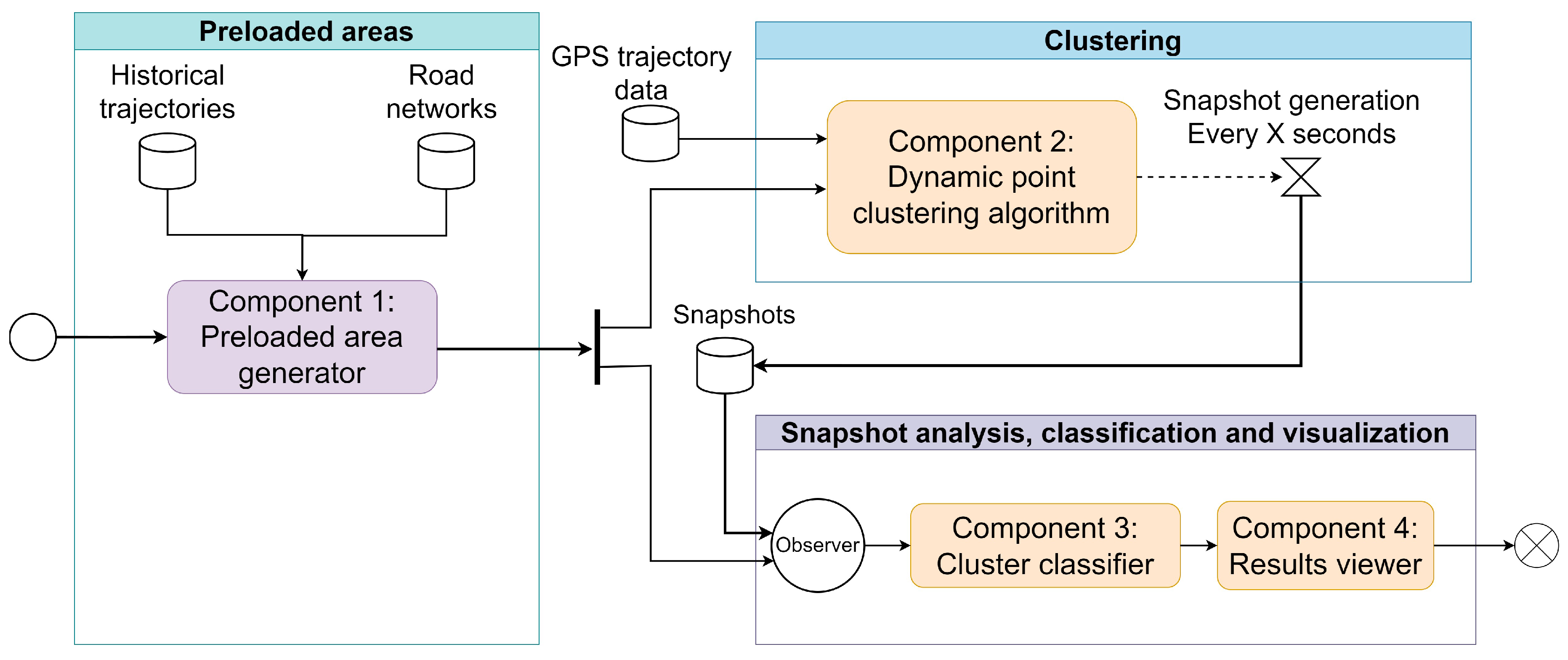
Figure 2.
Elements that compose a cluster.
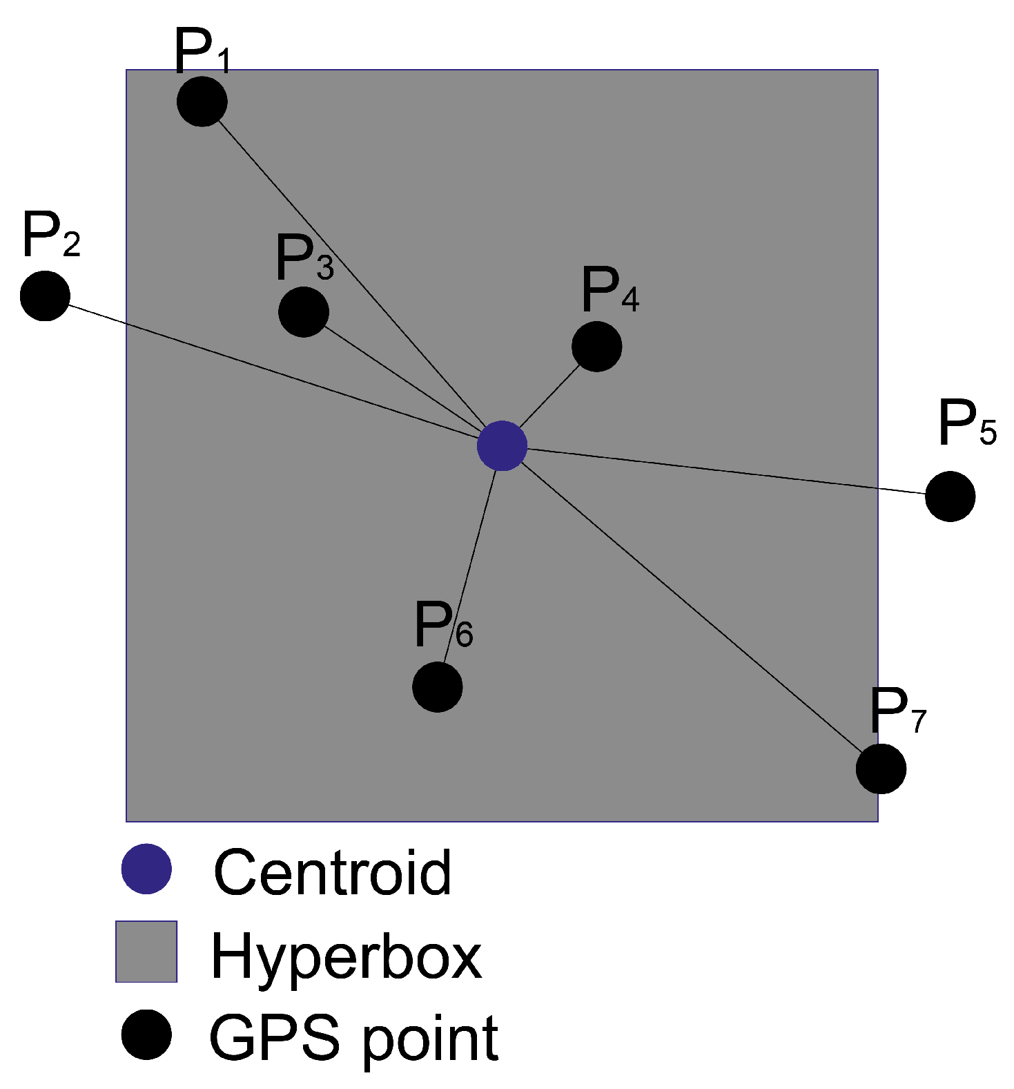
Figure 3.
Cluster-related information.
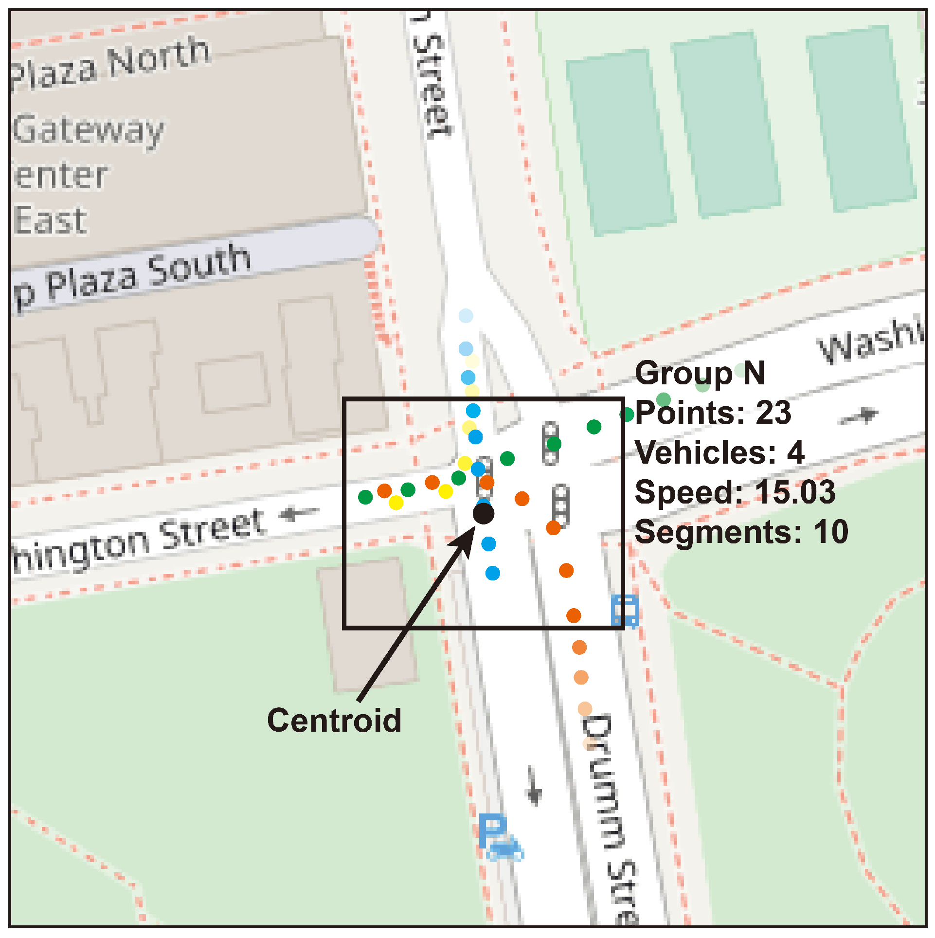
Figure 4.
Percentage of forgetting and relevance of data per unit of elapsed time for a lambda value set at 0.05.
Figure 4.
Percentage of forgetting and relevance of data per unit of elapsed time for a lambda value set at 0.05.
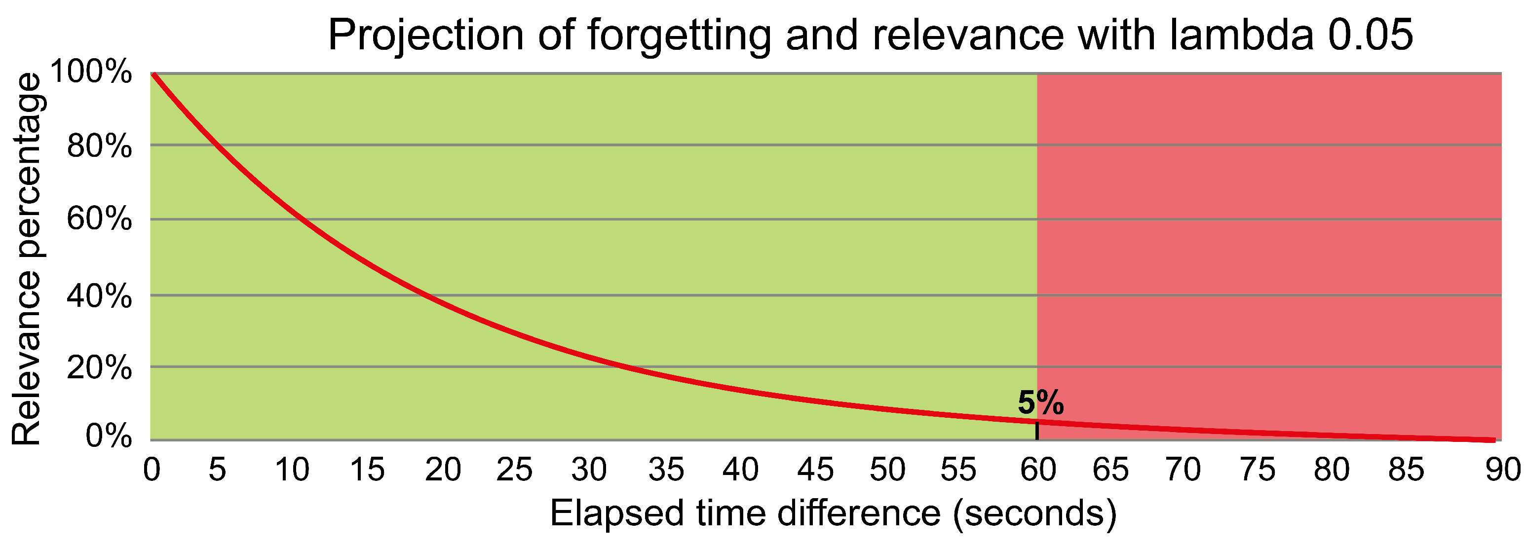
Figure 5.
Clusters projected on the map.
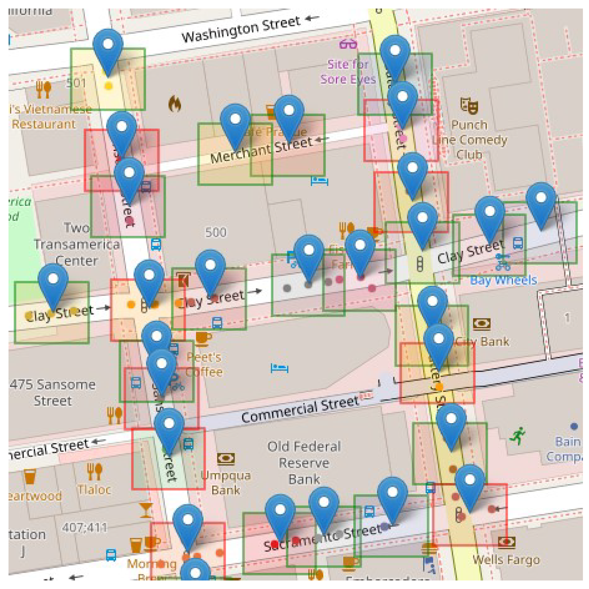
Figure 6.
Cluster projected on the grid.
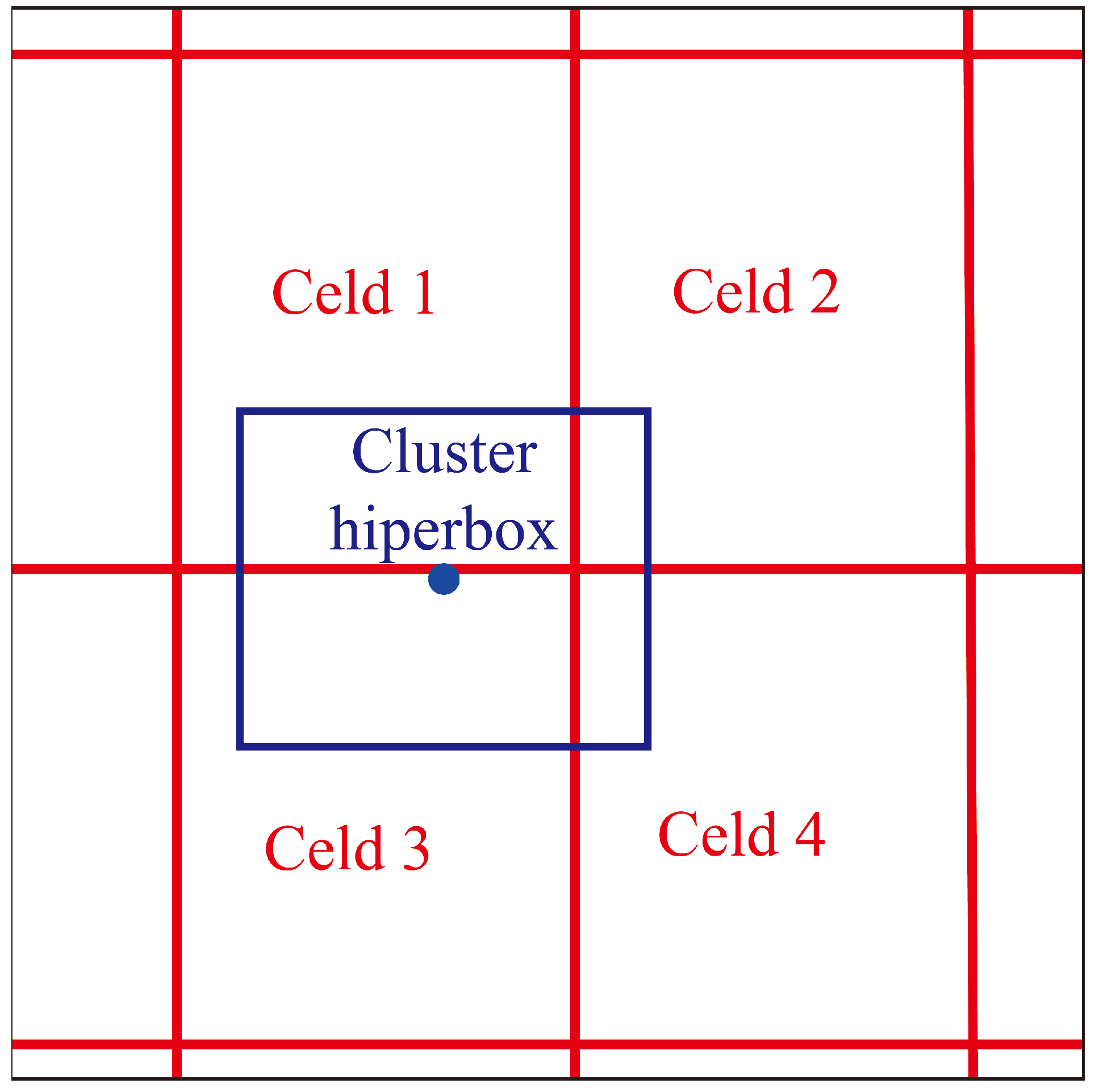
Figure 7.
Dynamism of a cluster as a function of elapsed time.
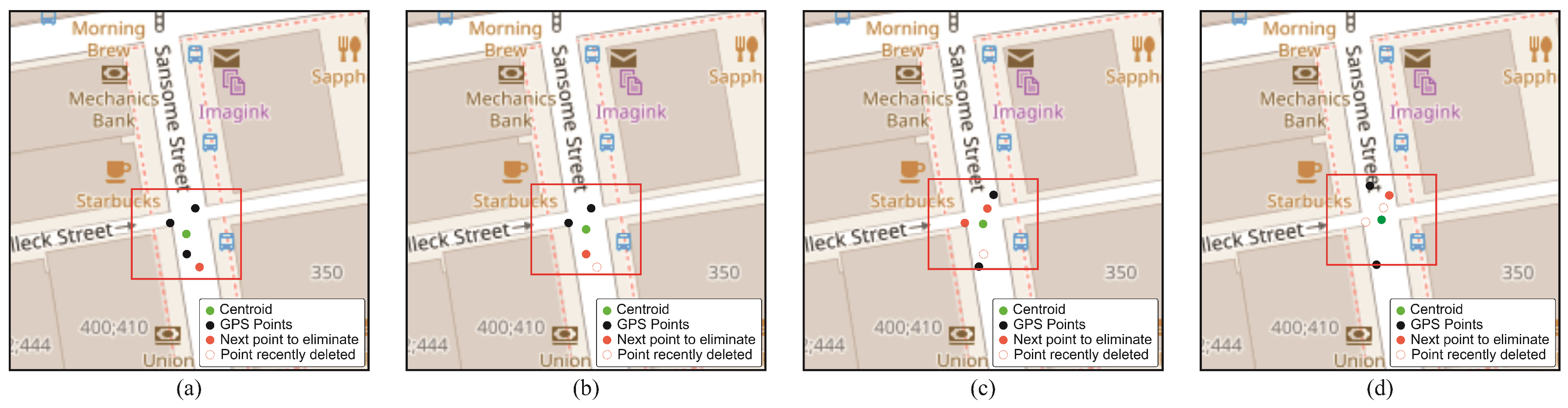
Figure 8.
Processed data flow in function of time.
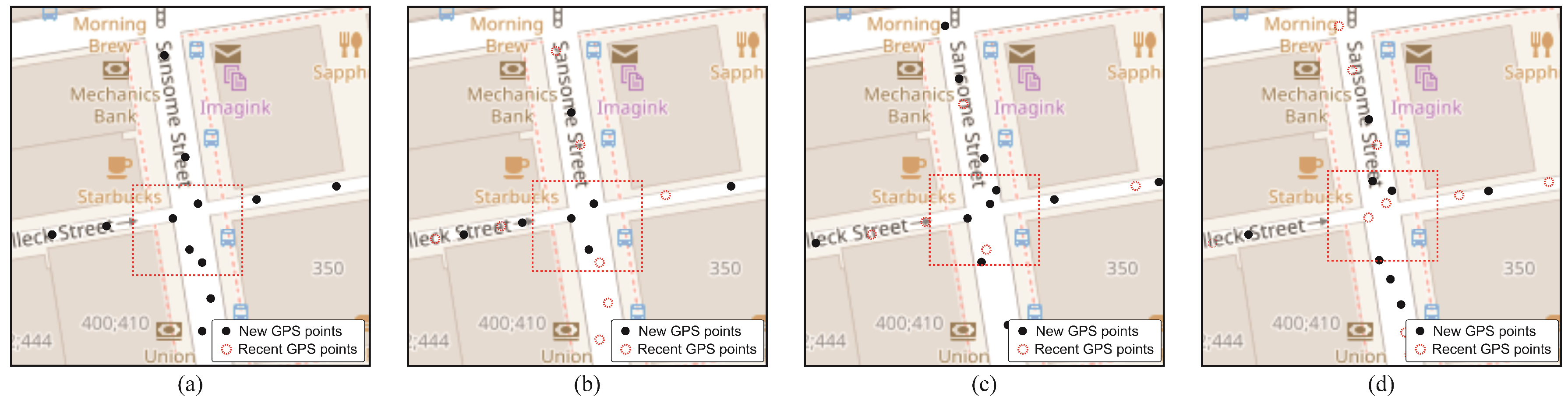
Figure 9.
Static grid showing the distribution of the cells that make it up.
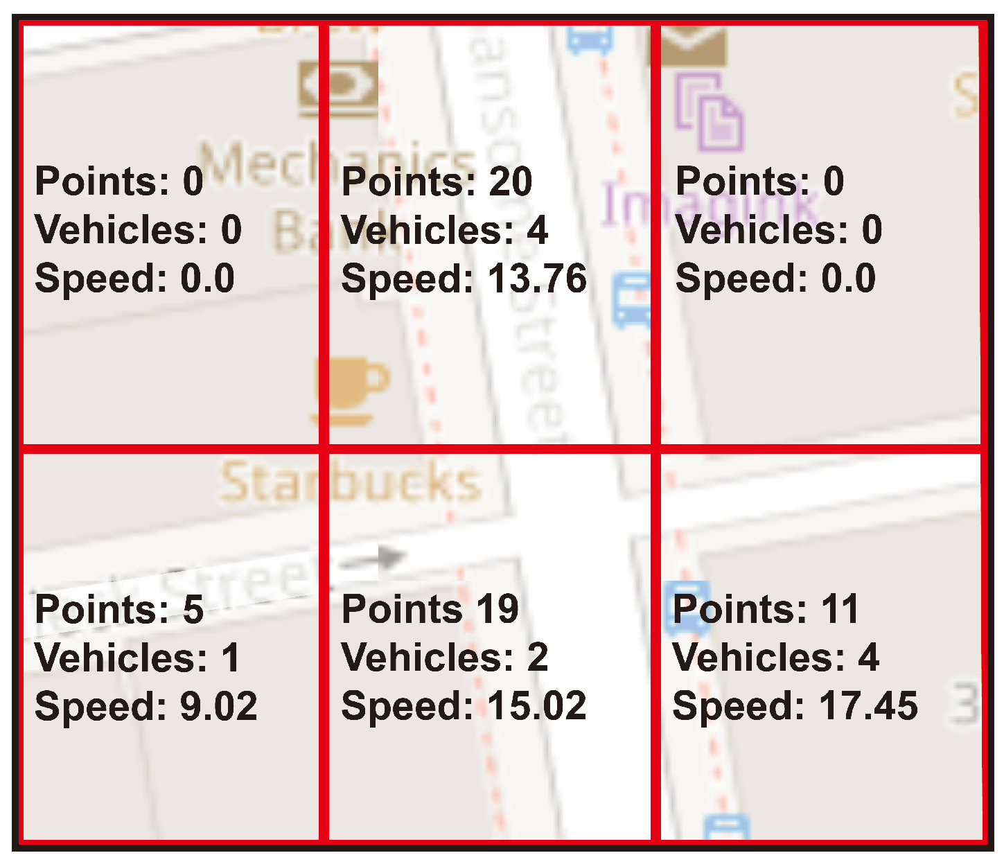
Figure 10.
Selection of dynamic road segments at the snapshots of minutes 1 (a), 3 (b) and 5 (c).
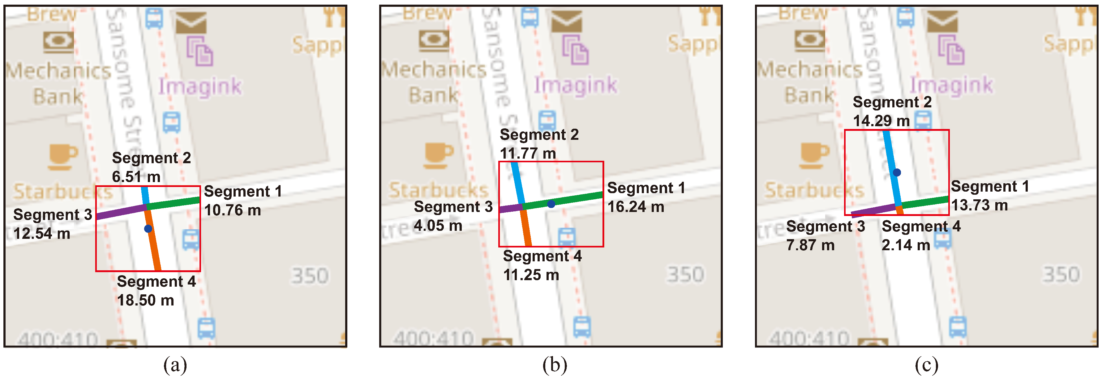
Figure 11.
Choosing road segments to establish fixed cells.
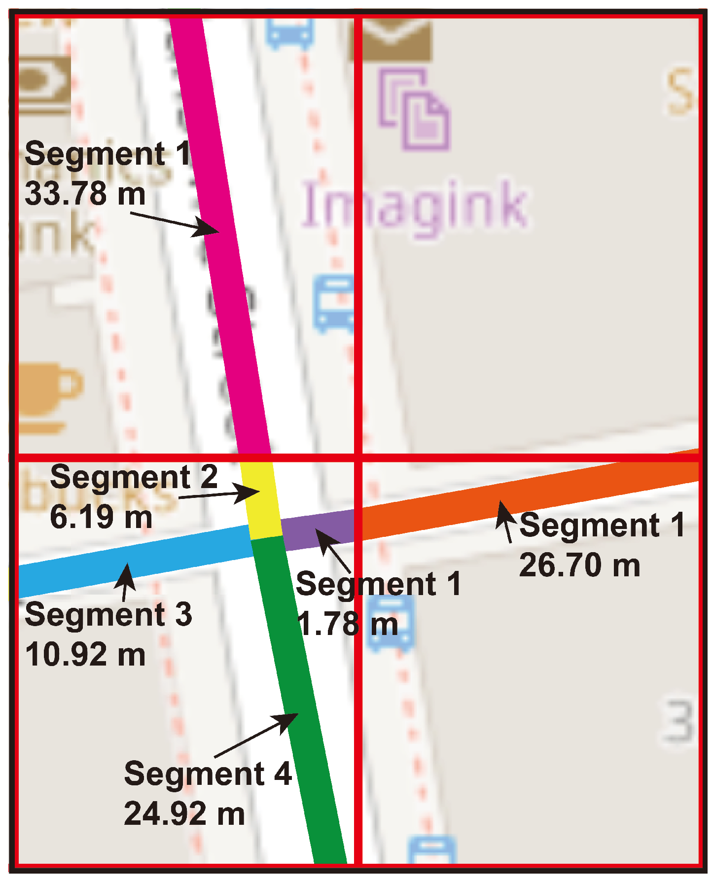
Figure 12.
Example of different network complexities: (a) A single road; (b) four roads; and (c) eleven roads.
Figure 12.
Example of different network complexities: (a) A single road; (b) four roads; and (c) eleven roads.
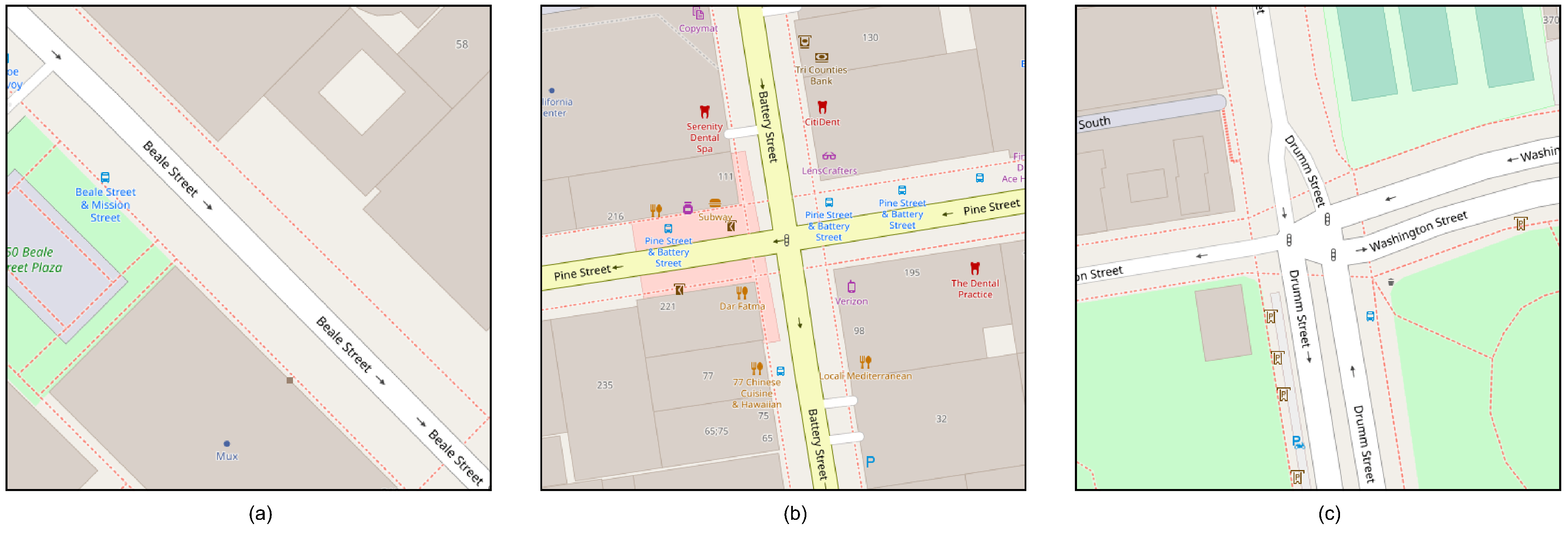

Table 1.
Execution times (minutes) of the proposed method for snapshots of 60 seconds.
| Component | San Francisco | Rome | Guayaquil |
|---|---|---|---|
| Clustering | 28:23 | 10:46 | 18:32 |
| Classification | 19:11 | 8:30 | 7:40 |
| Maximum time | 28:23 | 10:46 | 18:32 |
Table 2.
Execution times (minutes) of the proposed method for 30-second snapshots.
| Component | San Francisco | Rome | Guayaquil |
|---|---|---|---|
| Clustering | 27:34 | 11:02 | 18:37 |
| Classification | 39:01 | 15:13 | 31:41 |
| Maximum time | 39:01 | 15:13 | 31:41 |
Table 3.
Consolidated results using 60-second snapshots with the San Francisco data set.
| Tolerance | Cluster classification | Congested TCC | Non-congested TCC |
|---|---|---|---|
| 0.2 | Congested cluster | 11237 | 1748 |
| Non-congested cluster | 166 | 2503 | |
| 0.1 | Congested cluster | 10614 | 2371 |
| Non-congested cluster | 176 | 2492 | |
| 0 | Congested cluster | 10029 | 2956 |
| Non-congested cluster | 211 | 2457 |
Table 4.
Consolidated results using 30-second snapshots with the San Francisco data set.
| Tolerance | Cluster classification | Congested TCC | Non-congested TCC |
|---|---|---|---|
| 0.2 | Congested cluster | 14184 | 7062 |
| Non-congested cluster | 1227 | 3294 | |
| 0.1 | Congested cluster | 13335 | 7911 |
| Non-congested cluster | 1263 | 3258 | |
| 0 | Congested cluster | 12471 | 8775 |
| Non-congested cluster | 1287 | 3234 |
Table 5.
Consolidated results using 60-second snapshots with the Rome data set.
| Tolerance | Cluster classification | Congested TCC | Non-congested TCC |
|---|---|---|---|
| 0.2 | Congested cluster | 3195 | 309 |
| Non-congested cluster | 30 | 412 | |
| 0.1 | Congested cluster | 3089 | 415 |
| Non-congested cluster | 30 | 412 | |
| 0 | Congested cluster | 2994 | 510 |
| Non-congested cluster | 34 | 408 |
Table 6.
Consolidated results using 30-second snapshots with the Rome data set.
| Tolerance | Cluster classification | Congested TCC | Non-congested TCC |
|---|---|---|---|
| 0.2 | Congested cluster | 4689 | 2159 |
| Non-congested cluster | 390 | 509 | |
| 0.1 | Congested cluster | 4594 | 2254 |
| Non-congested cluster | 391 | 508 | |
| 0 | Congested cluster | 4497 | 2351 |
| Non-congested cluster | 399 | 500 |
Table 7.
Consolidated results using 60-second snapshots with the Guayaquil data set.
| Tolerance | Cluster classification | Congested TCC | Non-congested TCC |
|---|---|---|---|
| 0.2 | Congested cluster | 2576 | 276 |
| Non-congested cluster | 146 | 1912 | |
| 0.1 | Congested cluster | 2535 | 317 |
| Non-congested cluster | 167 | 1891 | |
| 0 | Congested cluster | 2459 | 393 |
| Non-congested cluster | 186 | 1872 |
Table 8.
Consolidated results using 30-second snapshots with the Guayaquil data set.
| Tolerance | Cluster classification | Congested TCC | Non-congested TCC |
|---|---|---|---|
| 0.2 | Congested cluster | 3364 | 1622 |
| Non-congested cluster | 1193 | 2328 | |
| 0.1 | Congested cluster | 3270 | 1716 |
| Non-congested cluster | 1209 | 2312 | |
| 0 | Congested cluster | 3155 | 1831 |
| Non-congested cluster | 1240 | 2281 |
Table 9.
Accuracy of the method.
| City | Tolerance | 60-second snapshots | 30-second snapshots |
|---|---|---|---|
| San Francisco | 0.2 | 87.77% | 67.83% |
| 0.1 | 83.73% | 64.40% | |
| 0 | 79.77% | 60.95% | |
| Rome | 0.2 | 91.41% | 67.10% |
| 0.1 | 88.72% | 65.86% | |
| 0 | 86.21% | 64.50% | |
| Guayaquil | 0.2 | 91.41% | 66.91% |
| 0.1 | 90.14% | 65.62% | |
| 0 | 88.21% | 63.90% |
Table 10.
Precision and recall of the congested category.
| City | Tolerance | 60-second snapshots | 30-second snapshots | ||
|---|---|---|---|---|---|
| Precision | Recall | Precision | Recall | ||
| San Francisco | 0.2 | 86.54% | 98.54% | 66.76% | 92.04% |
| 0.1 | 81.74% | 98.37% | 62.76% | 91.35% | |
| 0 | 77.24% | 97.94% | 58.70% | 90.65% | |
| Rome | 0.2 | 91.18% | 99.07% | 68.47% | 92.32% |
| 0.1 | 88.16% | 99.04% | 67.09% | 92.16% | |
| 0 | 85.45% | 98.88% | 65.67% | 91.85% | |
| Guayaquil | 0.2 | 90.32% | 94.64% | 67.47% | 73.82% |
| 0.1 | 88.88% | 93.82% | 65.58% | 73.01% | |
| 0 | 86.22% | 92.97% | 63.28% | 71.79% | |
Table 11.
Precision and precision of the non-congested category.
| City | Tolerance | 60-second snapshots | 30-second snapshots | ||
|---|---|---|---|---|---|
| Precision | Recall | Precision | Recall | ||
| San Francisco | 0.2 | 93.78% | 58.88% | 72.86% | 31.81% |
| 0.1 | 93.40% | 51.24% | 72.06% | 29.17% | |
| 0 | 92.09% | 45.39% | 71.53% | 26.93% | |
| Roma | 0.2 | 93.21% | 57.14% | 56.62% | 19.08% |
| 0.1 | 93.21% | 49.82% | 56.51% | 18.39% | |
| 0 | 92.31% | 44.44% | 55.62% | 17.54% | |
| Guayaquil | 0.2 | 92.91% | 87.39% | 66.12% | 58.94% |
| 0.1 | 91.89% | 85.64% | 65.66% | 57.40% | |
| 0 | 90.96% | 82.65% | 64.78% | 55.47% | |
Disclaimer/Publisher’s Note: The statements, opinions and data contained in all publications are solely those of the individual author(s) and contributor(s) and not of MDPI and/or the editor(s). MDPI and/or the editor(s) disclaim responsibility for any injury to people or property resulting from any ideas, methods, instructions or products referred to in the content. |
© 2024 by the authors. Licensee MDPI, Basel, Switzerland. This article is an open access article distributed under the terms and conditions of the Creative Commons Attribution (CC BY) license (http://creativecommons.org/licenses/by/4.0/).
Copyright: This open access article is published under a Creative Commons CC BY 4.0 license, which permit the free download, distribution, and reuse, provided that the author and preprint are cited in any reuse.


