

Submitted:
15 January 2024
Posted:
16 January 2024
Read the latest preprint version here
Abstract
We show that metallic ratios for real k are defined by an argument of a normalized complex number, while for rational k ≠ {0, ±2}, they are defined by Pythagorean triples. We further extend the concept of metallic ratios to metallic angles.
Keywords:
metallic ratios
; Pythagorean triples
; emergent dimensionality
; mathematical physics
1. Introduction
Each rectangle contains at least one square with an edge h equal to the shorter edge of the rectangle. If a rectangle contains k such squares and its edges and h satisfy
they satisfy a metallic ratio; the golden ratio for , the silver ratio for , shown in Figure 1, the bronze ratio for , etc.
Because the edge lengths of a metallic rectangle are assumed to be nonnegative, usually only the positive principal square root of (2) is considered. However, distance nonnegativity (corresponding to the ontological principle of identity of indiscernibles) does not hold for the Ł–K metric [1], for example; such an axiomatization is misleading [2].
Metallic ratios (3) have interesting properties, such as
Furthermore, as k goes to ifinity, the factor in the square root becomes negligible, and for large k.
It was shown [3] that for positive metallic ratios (3) can be expressed by primitive Pythagorean triples, as
and for
where is the angle between a longer cathetus b and hypotenuse c of a right triangle defined by a Pythagorean triple, as shown in Figure 3, whereas for it is the angle between a hypotenuse and a shorter cathetus a ( and are defined by the same Pythagorean triples, respectively, and ), and
For example the Pythagorean triple defines , the Pythagorean triple defines , the Pythagorean triple defines , and so on.
2. Results
Theorem 1.
The metallic ratio of is defined by an acute angle of a right triangle .
Proof.
We express the RHS of the Equation (5) using half-angle formulas and substituting
since (we exclude degenerated triangles), so .
We can extend the domain of Theorem 1 by analytic continuation to as in this range. However, extending it further to we note that in this range . Thus, the quadratic Equation (9) becomes
and its roots are
Theorem 2.
The metallic ratio of is defined by an angle .
Proof.
Equations (14) and (16) relate which defines a metallic ratio (3) to the normalized complex number . The angles and are shown in Figure 4. There are two axes of symmetry.
In summary, metallic ratios as functions of are
where the first ± defines the range of and the second ± corresponds to positive or negative form of the ratio. Therefore, the first and second properties (4) hold for and but the third property (4) holds as .
Proof.
Plugging rational into the relation (14) gives
and is a possible solution. It is easy to see that . implies and valid . implies and also valid . □
Table 1 shows the generalized Pythagorean triples that define the metallic ratios for .
3. Metallic Angles
We can extend the concept of metallic ratios (1) to angles as
where for well known golden angle , shown in Figure 6, is obtained.
In this case, their products and sums
are dependent on k, where and .
Acknowledgments
I thank my wife Magdalena Bartocha for her unwavering motivation and my friend, Renata Sobajda, for her prayers.
References
- Łukaszyk, S. A new concept of probability metric and its applications in approximation of scattered data sets. Computational Mechanics 2004, 33, 299–304. [Google Scholar] [CrossRef]
- Łukaszyk, S.; Tomski, A. Omnidimensional Convex Polytopes. Symmetry 2023, 15, 755. [Google Scholar] [CrossRef]
- Rajput, C. Metallic Ratios in Primitive Pythagorean Triples : Metallic Means embedded in Pythagorean Triangles and other Right Triangles. JOURNAL OF ADVANCES IN MATHEMATICS 2021, 20, 312–344. [Google Scholar] [CrossRef]
Figure 1.
Silver ratio .
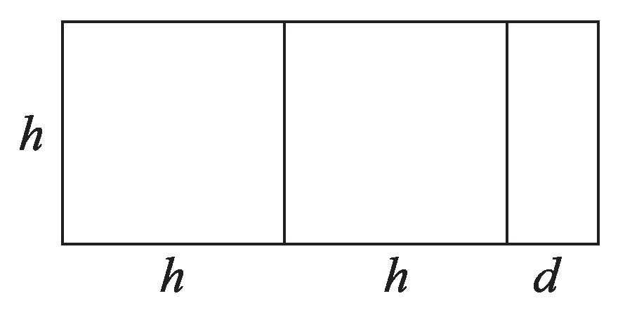
Figure 2.
Metallic ratios: positive (red), negative (green) as continuous functions of .
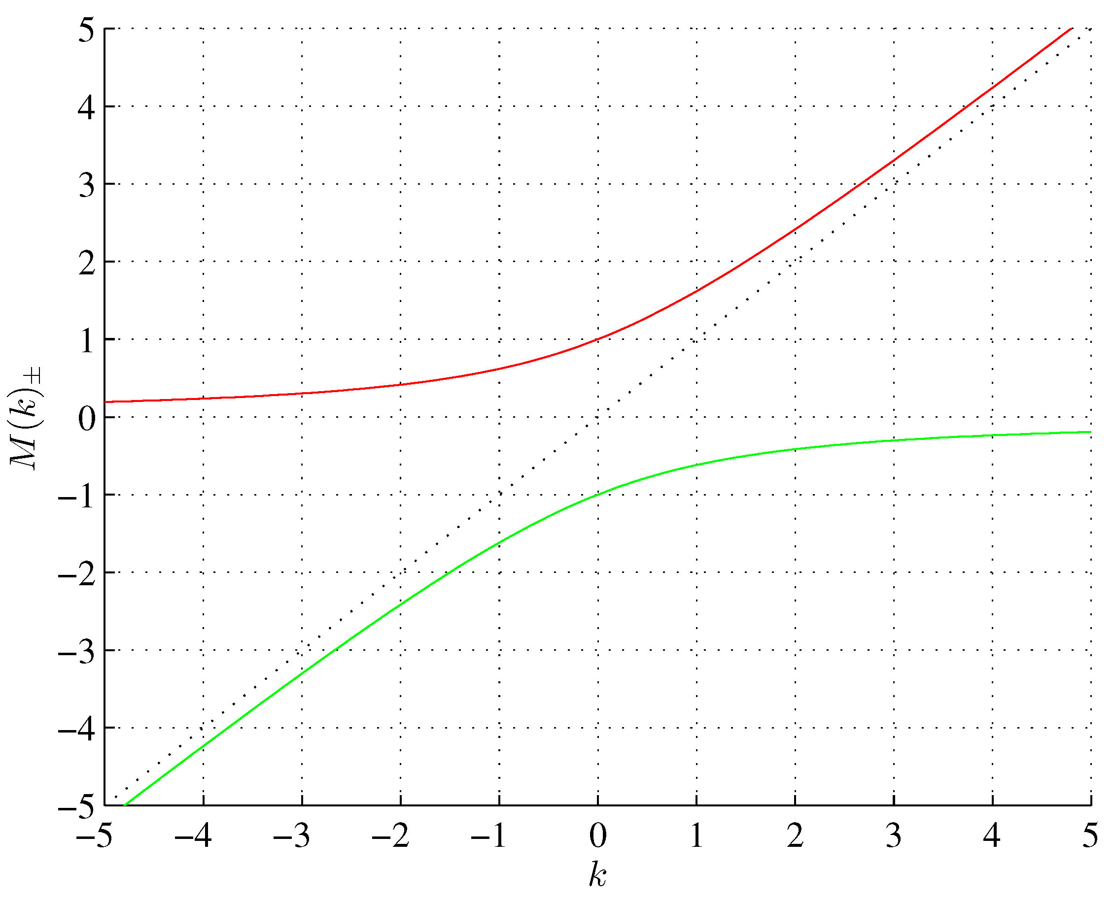
Figure 3.
Right triangle showing a longer (b), shorter (a) hypotenuse, catheti (c) and angles and .
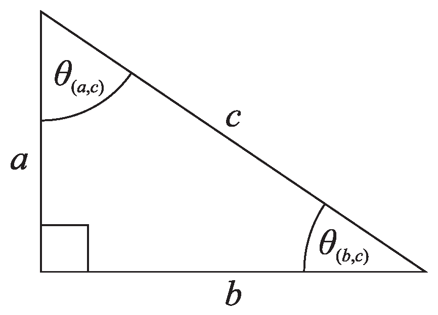
Figure 4.
Phases of the complex number (red, ) and its conjugate (green, ) for . , .
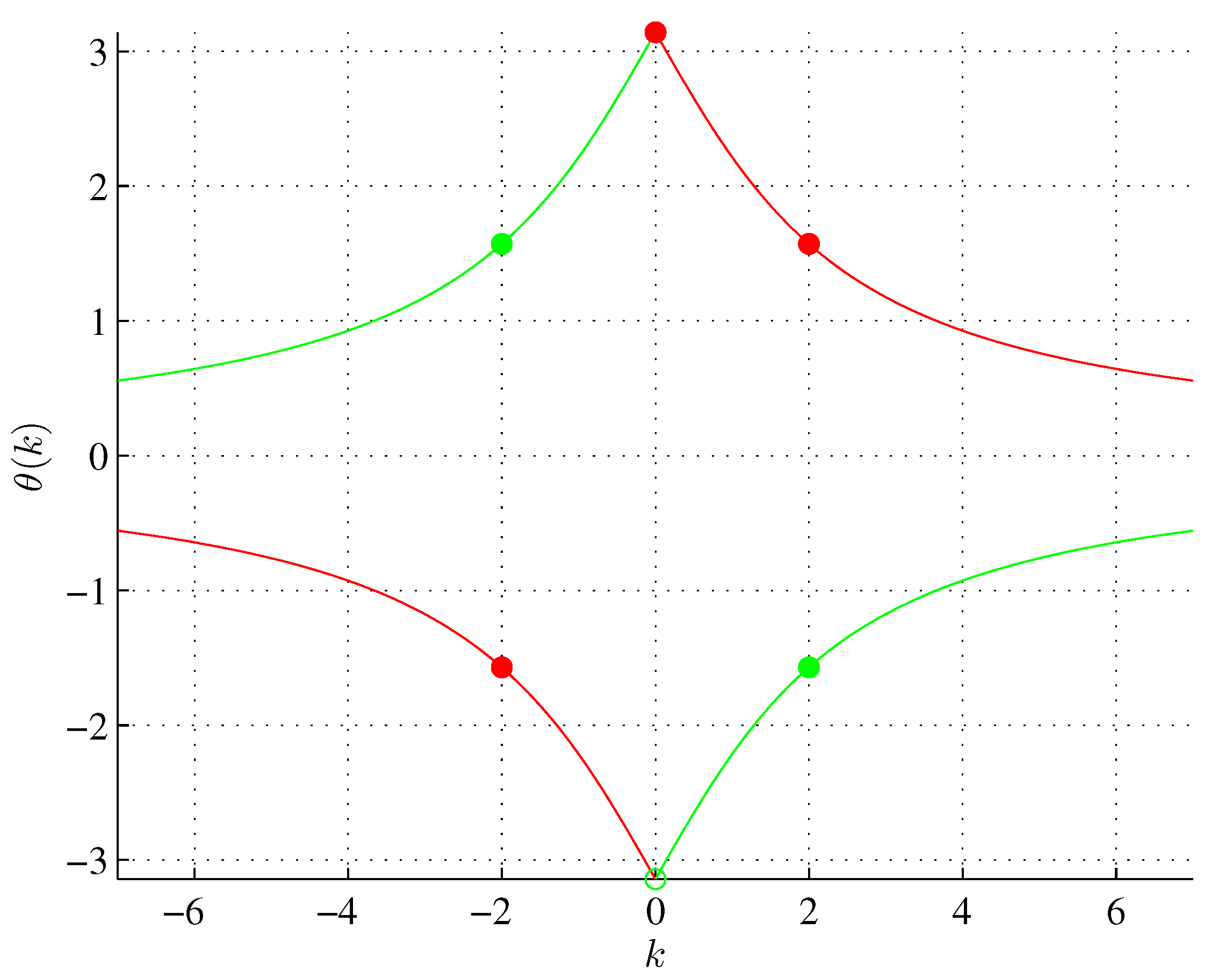
Figure 5.
Metallic ratios: positive (red), negative (green) as a function of (dotted), and (solid), and (positive: solid blue; negative: solid cyan) for .
Figure 5.
Metallic ratios: positive (red), negative (green) as a function of (dotted), and (solid), and (positive: solid blue; negative: solid cyan) for .
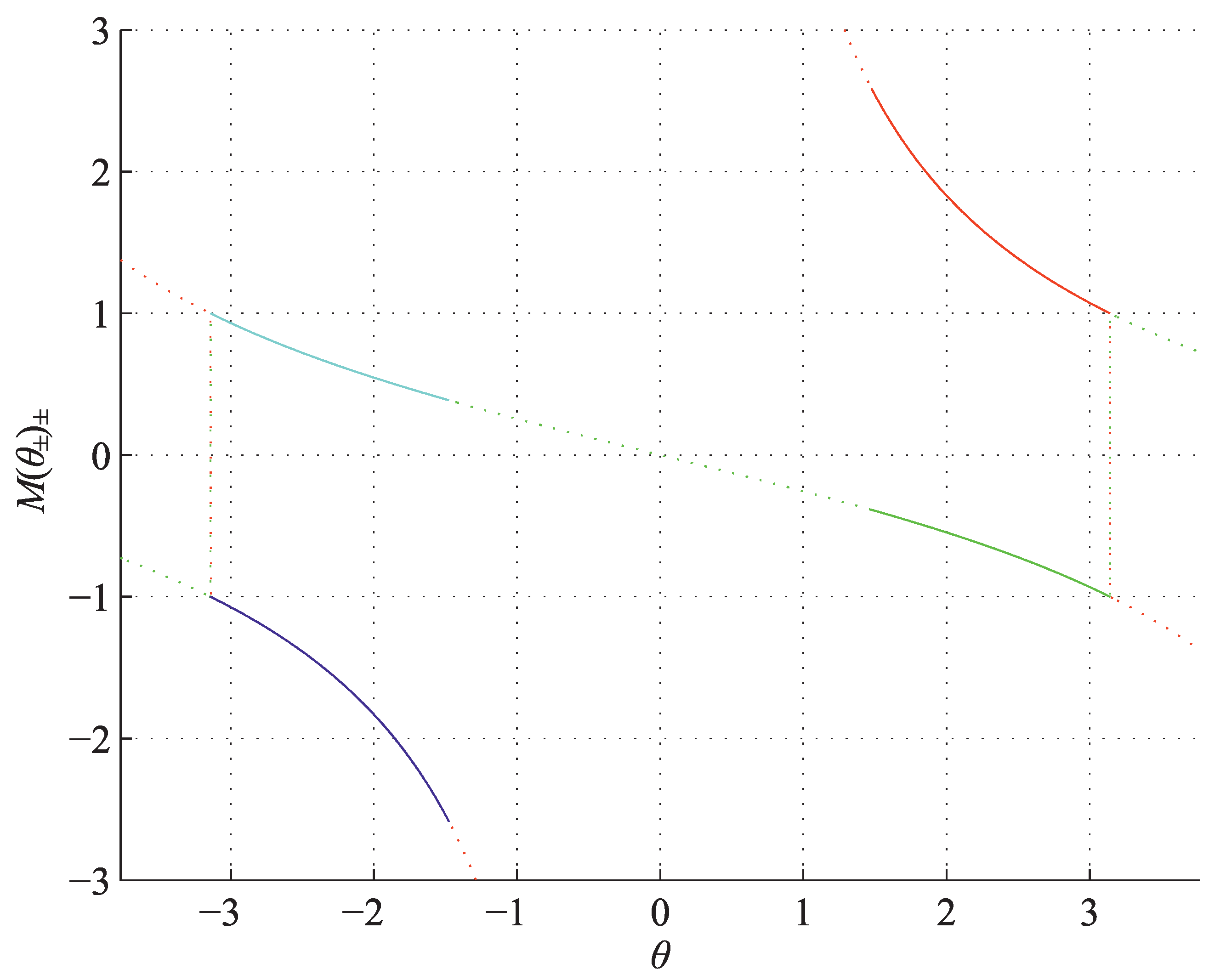
Figure 6.
Golden angle .
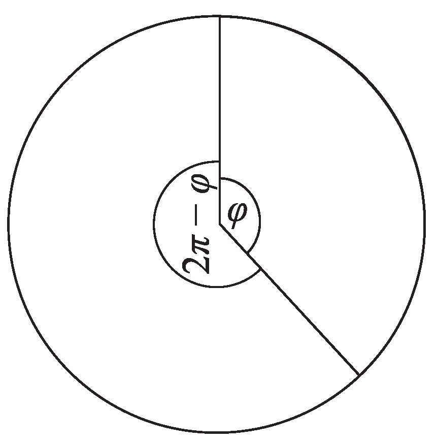
Figure 7.
Metallic angles (solid) and ratios (dotted), positive (red), negative (green), as continuous functions of .
Figure 7.
Metallic angles (solid) and ratios (dotted), positive (red), negative (green), as continuous functions of .
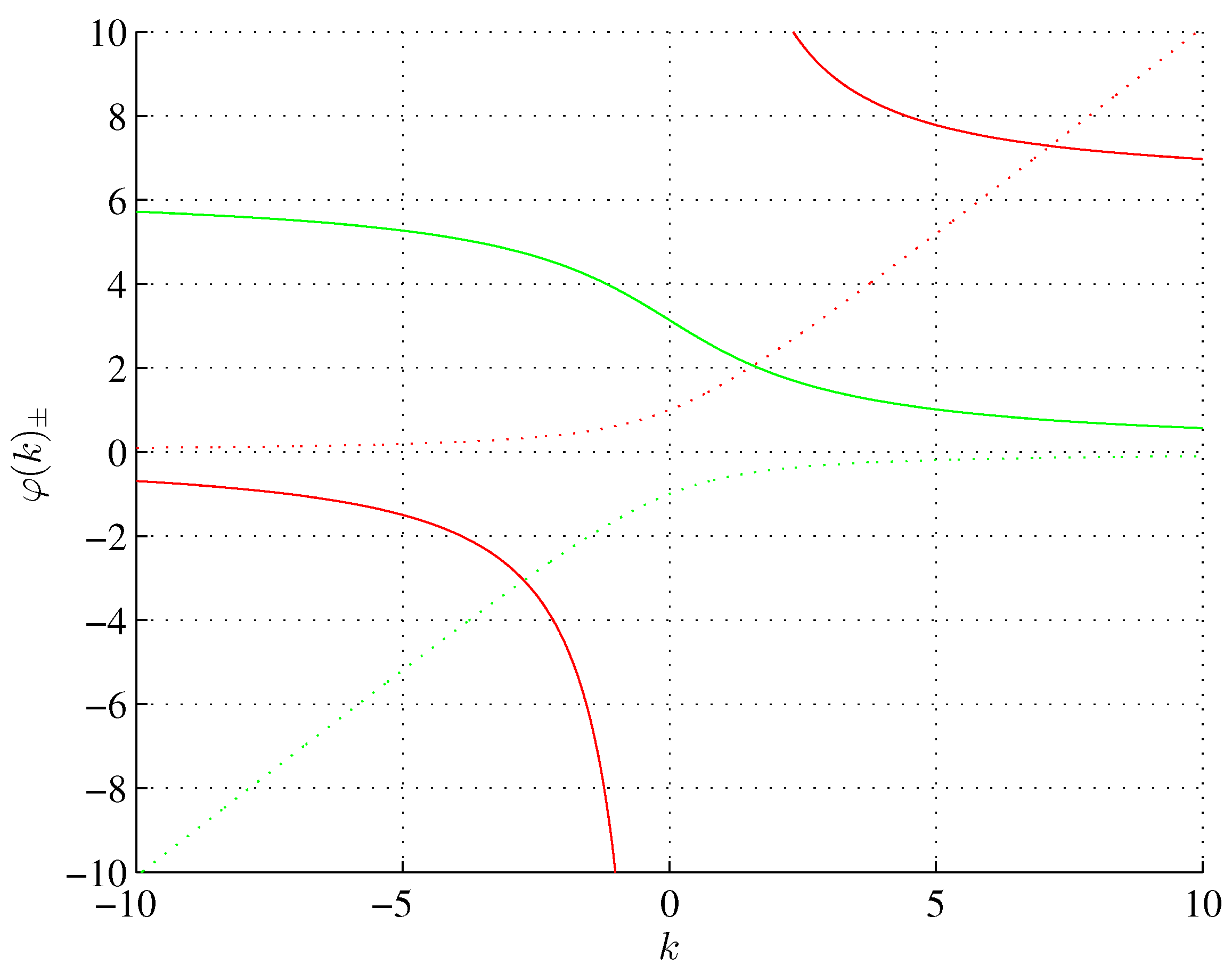

Table 1.
Pythagorean triples associated with metallic ratios for rational .
| k | a | b | c | k | a | b | c |
|---|---|---|---|---|---|---|---|
| 0.1 | −399 | 40 | 401 | 3.6 | 28 | 45 | 53 |
| 0.2 | −99 | 20 | 101 | 3.7 | 969 | 1480 | 1769 |
| 0.3 | −391 | 120 | 409 | 3.8 | 261 | 380 | 461 |
| 0.4 | −12 | 5 | 13 | 3.9 | 1121 | 1560 | 1921 |
| 0.5 | −15 | 8 | 17 | 4 | 3 | 4 | 5 |
| 0.6 | −91 | 60 | 109 | 4.1 | 1281 | 1640 | 2081 |
| 0.7 | −351 | 280 | 449 | 4.2 | 341 | 420 | 541 |
| 0.8 | −21 | 20 | 29 | 4.3 | 1449 | 1720 | 2249 |
| 0.9 | −319 | 360 | 481 | 4.4 | 48 | 55 | 73 |
| 1 | −3 | 4 | 5 | 4.5 | 65 | 72 | 97 |
| 1.1 | −279 | 440 | 521 | 4.6 | 429 | 460 | 629 |
| 1.2 | −8 | 15 | 17 | 4.7 | 1809 | 1880 | 2609 |
| 1.3 | −231 | 520 | 569 | 4.8 | 119 | 120 | 169 |
| 1.4 | −51 | 140 | 149 | 4.9 | 2001 | 1960 | 2801 |
| 1.5 | −7 | 24 | 25 | 5 | 21 | 20 | 29 |
| 1.6 | −9 | 40 | 41 | 5.1 | 2201 | 2040 | 3001 |
| 1.7 | −111 | 680 | 689 | 5.2 | 72 | 65 | 97 |
| 1.8 | −19 | 180 | 181 | 5.3 | 2409 | 2120 | 3209 |
| 1.9 | −39 | 760 | 761 | 5.4 | 629 | 540 | 829 |
| 2 | 5.5 | 105 | 88 | 137 | |||
| 2.1 | 41 | 840 | 841 | 5.6 | 171 | 140 | 221 |
| 2.2 | 21 | 220 | 221 | 5.7 | 2849 | 2280 | 3649 |
| 2.3 | 129 | 920 | 929 | 5.8 | 741 | 580 | 941 |
| 2.4 | 11 | 60 | 61 | 5.9 | 3081 | 2360 | 3881 |
| 2.5 | 9 | 40 | 41 | 6 | 4 | 3 | 5 |
| 2.6 | 69 | 260 | 269 | 6.1 | 3321 | 2440 | 4121 |
| 2.7 | 329 | 1080 | 1129 | 6.2 | 861 | 620 | 1061 |
| 2.8 | 12 | 35 | 37 | 6.3 | 3569 | 2520 | 4369 |
| 2.9 | 441 | 1160 | 1241 | 6.4 | 231 | 160 | 281 |
| 3 | 5 | 12 | 13 | 6.5 | 153 | 104 | 185 |
| 3.1 | 561 | 1240 | 1361 | 6.6 | 989 | 660 | 1189 |
| 3.2 | 39 | 80 | 89 | 6.7 | 4089 | 2680 | 4889 |
| 3.3 | 689 | 1320 | 1489 | 6.8 | 132 | 85 | 157 |
| 3.4 | 189 | 340 | 389 | 6.9 | 4361 | 2760 | 5161 |
| 3.5 | 33 | 56 | 65 | 7 | 45 | 28 | 53 |
For set . E.g. for k = −7, {45, 28, 53} ↔ {45,−28, 53}.
Disclaimer/Publisher’s Note: The statements, opinions and data contained in all publications are solely those of the individual author(s) and contributor(s) and not of MDPI and/or the editor(s). MDPI and/or the editor(s) disclaim responsibility for any injury to people or property resulting from any ideas, methods, instructions or products referred to in the content. |
© 2024 by the authors. Licensee MDPI, Basel, Switzerland. This article is an open access article distributed under the terms and conditions of the Creative Commons Attribution (CC BY) license (http://creativecommons.org/licenses/by/4.0/).
Copyright: This open access article is published under a Creative Commons CC BY 4.0 license, which permit the free download, distribution, and reuse, provided that the author and preprint are cited in any reuse.