Submitted:
04 January 2024
Posted:
05 January 2024
You are already at the latest version
Abstract
The relativistic Doppler effect comes from the fact that observers in different inertial reference frames experience space and time differently, while the speed of light remains always the same. Consequently, a wave packet of light exhibits different frequencies, wavelengths, and amplitudes. In this paper, we present a local approach to the relativistic Doppler effect based on relativity, spatial and time translational symmetries, and energy conservation. Afterward, we investigate the implications of the relativistic Doppler effect for the quantum state transformations of wave packets of light and show that a local photon is a local photon at the same point in the spacetime diagram in all inertial frames.
Keywords:
relativistic quantum information
; quantum electrodynamics
; quantum photonics
1. Introduction
When a moving car beeps its horn, the driver and a bystander on the pavement hear the sound at different frequencies. The frequency shift resulting from the relative motion of the driver and the bystander is known as the Doppler effect [1,2] and is well understood in classical physics. For example, the frequency heard by the resting observer depends on the speed of the car relative to the pavement and the original frequency of the signal. Due to its simplicity, the Doppler effect has already found a wide range of applications, including the policing of speed limit violations by irresponsible drivers. The relativistic Doppler effect [3,4,5,6,7,8,9] also accounts for differences in how observers experience space and time. Observers in different inertial reference frames which move at a relative speed close to the speed of light receive signals which differ not only in frequency and wavelength but also in amplitude.
According to Einstein’s principle of relativity [10,11,12,13,14,15,16], there is no privileged frame of reference. The same physical laws apply in all reference frames if these move with respect to each other at constant velocity. For example, wave packets of light with a well-defined direction of propagation move at the speed of light, c, in any reference frame. Some authors might still debate whether this assumption is true or not [17] but many experiments already verified the constancy of the speed of light with high accuracy [18,19]. Moreover, any physical theory that involves space and time requires a way of measuring both using clocks and meters. In the following, we assume that all clocks and meters are calibrated such that light travels at the same speed in all reference frames. We then have a fresh look at the relativistic Doppler effect [5] with only a minimum of assumptions.
Instead of considering frequency space, in this paper we study the relativistic Doppler effect [3,5,6,7,8] in position space [20,21,22,23]. As we shall see below, this space can accommodate spatial and time translational symmetries in a straightforward way. Although our results are consistent with the existing literature [24,25,26,27,28,29,30,31,32], our approach paves the way for systematic studies of more complex scenarios, like the Unruh effect [33,34] and quantum electrodynamics in reference frames with time-varying accelerations without the need for approximations, such as the usual assumption of a flat spacetime [35]. Moreover, the insights obtained here might have applications in relativistic quantum information [36,37,38,39,40,41]. In the following, we review the relativistic Doppler effect before studying its implications for the quantised electromagnetic (EM) field in different inertial reference frames.
Suppose an observer—let us call her Alice (A)—is watching a wave packet of light with a well-defined direction of propagation s and a well-defined polarisation traveling along the x axis. Then the electric field amplitudes seen by Alice at positions at times equal
if the initial electric field amplitudes of the wave packet are given by . Here and correspond to wave packets propagating in the direction of decreasing and increasing respectively. Hence, if the physical properties of a wave packet seen by Alice are known at one instant in time, they are known at all times. The same applies to the electric field amplitudes seen at by a second observer—who we call Bob (B)—and
in analogy to Equation (1). The electric field observables perceived by both Alice and Bob at any position and time are only characterised by the value of the parameters with . In the remainder of this paper, we shall use a shorthand notation and replace by .
The principle of relativity also suggests that the electric and magnetic field transformations from observer A to observer B and vice versa need to be formally the same. The only difference is that the relative speed of their reference frames changes from to . This suggests a linear dependence between electric field amplitudes and at the same point in the spacetime diagram since this transformation is the only transformation which remains formally the same when reversed. We therefore assume in the following that
where the coordinates and specify the same spacetime trajectory and denotes a transformation constant. Analogously, we also know that
The principle of relativity also tells us that the transformation constants and relate to each other such that
since the direction of propagation s of the wave packet is the same in both reference frames, but the relative speed of the frames changes sign. When combining Equations (3)–(5) we therefore find that
In the following, this is taken into account when we determine and .
Next we notice that the spatial and time translational symmetries of the EM field tell us that the above relations must hold for all spacetime coordinates. Hence the transformation factors and can only depend on the direction of propagation s of the wave packet and on the relative speed of Bob’s reference frame with respect to Alice’s reference frame and not on where and when electric and magnetic field amplitudes are measured. The above arguments thus reduce the question, how do local electric and magnetic field observables transform from one inertial frame to another, to the simpler question, namely, how do the field observables transform at a single point in the spacetime diagram? Unfortunately, the above equations are not enough to determine the transformation factor in Equation (3). An additional assumption is needed.
Our final assumption in the derivation of the relativistic Doppler effect is based on energy conservation. To implement this we consider a “box” that moves at the speed of light along the x axis in the reference frame of observer B. By integrating over the volume inside the “box” at a fixed time we can calculate the amount of energy it contains. As the “box” propagates at the speed of light, any light initially caught inside or outside of that “box” will remain here for all time, and the total energy that it encloses will be conserved. Nevertheless, as Alice and Bob experience space and time differently, the “box” observed by Bob will appear deformed to Alice and the energy of the field will be measured differently. For example, parts of the wave packet that occur simultaneously in the frame of observer A appear at different times in the reference frame of observer B. Taking this into account, we can finally identify the dependence of and on s and on . When applying Fourier transforms to local electric field amplitudes, we obtain the usual momentum changes of the relativistic Doppler effect.
As mentioned already above, the main purpose of this paper is to obtain a simple quantum picture of the relativistic Doppler effect. In the following we use a local photon approach and proceed as described in Refs. [20,21,22] to quantise the EM field in different inertial reference frames. Given the principle of relativity, neither observer A nor observer B should be able to perform measurements on photonic wave packets which tell them about their relative speed. Taking this into account, we find that the local photon annihilation operators of Alice and Bob are the same when they refer to the same location in the spacetime diagram. However, the transformation of the annihilation operators of monochromatic photons is more complex. As we will see below, both observers Alice and Bob need to assign different quantum states and to wave packets of light, even when describing the same wave packet.
This paper is structured as follows. Section 2 reviews the relativistic Doppler effect in classical physics. We first study how the coordinates and of two inertial observers A and B relate to each other when they correspond to the same point in the spacetime diagram. Afterwards, we derive the electric field transformation rates and in Equations (1) and (2) by imposing the above described conditions. Section 3 reviews a local description of the quantised EM field [21,22] for light propagation in one dimension. Section 4 combines this description with the results of Section 2 to obtain a quantum picture of the relativistic Doppler effect and to identify the relationship between the quantum states and of a wave packet of light seen by observers A and B in different inertial frames. Finally, we summarise our findings in Section 5.
2. The Relativistic Doppler Effect
The motion of an observer affects both the time and distance separating two events in spacetime, as well as their electric and magnetic field observables. The change in duration and separation between events can be expressed as a transformation between the natural coordinates of the two observers involved; one taken as a reference observer. In this section, we provide a derivation of the coordinate transformations between an observer at rest and an observer moving with constant velocity. Afterwards, we use these coordinate transformations to determine the transformation constant in Equation (3).
2.1. Coordinate Transformations
In this paper we consider two observers, Alice and Bob, in a flat 1+1 dimensional spacetime (Minkowski space). In the following, we assume our first observer, Alice, who will provide a point of reference, to be at rest. Our second observer, Bob, is travelling at a constant velocity relative to Alice along the axis, as illustrated in Figure 1. The position and time at which an event takes place from Alice’s point of view are denoted and respectively. Analogously, from Bob’s point of view, events take place at a position at a time . For simplicity, we assume that both observers, who are stationary with respect to their own position coordinates, are located at the origin of these coordinates. This means that we choose Alice’s position to be for all times , while Bob’s position equals for all . Moreover, we assume in the following that Alice’s and Bob’s spacetime diagrams overlap at the origin. Hence Bob meets Alice only once at the initial time .
As mentioned already in the Introduction, in a stationary reference frame, Maxwell’s equations tell us that light propagates along the axis at the speed of light c. Therefore, if Alice sends a localised pulse of light to Bob, she will observe that its position at any time satisfies the relation
with . Physically, is the position of the light pulse at . The speed of light measured relative to the rest frame of an inertial observer is always constant and independent of the motion of the source. Hence, from Bob’s point of view, the position of the light pulse at any time satisfies the relation
with . Here may not be equal to , but the direction of propagation s of the light pulse must be the same in both reference frames. As both Equations (7) and (8) must be satisfied simultaneously for a single light pulse, it can be shown that
The relating constant may depend on s and provides a connection between the coordinates adopted by Alice and the ones adopted by Bob. The difference in the way position and time are perceived by Alice and Bob has a crucial influence on the way electric and magnetic fields are measured. The aim of this subsection, therefore, is to determine the factor in Equation (9).
Suppose Alice sends a short light pulse from her own position at at a time to Bob, as illustrated in Figure 1. From Bob’s point of view, the light is emitted from a position at a time and arrives at Bob’s position when his watch reads a time . As Alice’s and Bob’s positions are always zero in their respective reference frames, Equation (9) tells us that
This relation takes into account both the time it takes the light to propagate from Alice to Bob and any difference in the rate at which their clocks are running. To determine the relation between and and between and , respectively, we consider the spacetime diagrams for the experiment from both Alice’s and Bob’s points of view. As illustrated in Figure 2, according to Alice’s measurements, Bob receives the light pulse at a position at a time with . As Bob travels at a constant speed with respect to Alice, the position of Bob when the signal is received is . Putting these two relations together, we find that
with . Moreover, from Bob’s point of view, Alice travels to the left with a velocity . Hence , which leads to
Equations (11) and (12) specify the relationship between the times at which the light is emitted and received from the points of view of both observers.
In Bob’s reference frame, the time elapsed between two events may not be the same as the time elapsed between the same events in Alice’s frame [11,12,13,14]. In general, a moving clock will tick at a different rate than a stationary clock, and we must consider this. According to Alice, the position at which the signal is received varies with time, whereas for Bob it does not. If a moving clock ticks more slowly than a stationary one by a rate of , then it follows that [15,16]
As the position of the emitter is stationary with respect to Alice but moving at a constant velocity with respect to Bob, it must also be that
Since is always larger than 1, clocks run slower in a moving frame.
By putting together Equations (12) and (14) the factor can be determined. We find that for light propagating to the right where is defined in Equation (15). By carrying out a similar set of calculations for left-propagating light that is transmitted by Alice at some time we can determine the complete relation
The two equations (one for each value of s) given in Equation (16) relate the trajectory of a light pulse in Bob’s reference frame to a light pulse in Alice’s reference frame. What is more, by solving these equations we can derive the point-like coordinate transformations for and . The equations
establish a connection between spacetime coordinates and which refer to the same point in the spacetime diagram.
2.2. Field Amplitude Transformations
Since Alice and Bob perceive space and time differently (cf. Equation (17)), wave packets of light appear to have different shapes in each reference frame. What is more, the electric and magnetic field amplitudes of wave packets differ for Alice and Bob even at points which correspond to the same location in the spacetime diagram. This means that the same wave packet carries a different amount of energy from the point of view of Alice than it does from the point of view of Bob. Despite these changes, we know that light carries a conserved and invariant energy flux . Here is a vector which points along the trajectory of light in the spacetime diagram and whose amplitude quantifies the total amount of energy that is moving in this direction. Since the speed of light is the same in all reference frames, a component of this energy flux will always intersect the and position axes. It is these components that correspond to the energy of the EM field as measured by Alice and Bob and relate closely to their field amplitudes. Hence in this subsection, we use energy flux conservation to identify the field amplitude transformations between inertial frames, i.e., the factor in Equation (3).
Suppose that a short light pulse propagating through spacetime is confined to a “box” that propagates along the x-axis at the speed of light in the same direction as the wave packet. The light pulse remains confined to this “box” in all reference frames. Suppose that the edge of the “box” is parallel to the axis in Bob’s reference frame and that it has the length as illustrated in Figure 3(a). Figure 3(b) shows the same “box” from the point of view of Alice. Here the “box” also travels at the speed of light, but is deformed. Most importantly, any light initially in the “box” cannot exit and any light outside cannot enter. Hence the energy flux within the “box” must be the same in both reference frames.
To take advantage of the invariance of , we notice that the EM field energy seen by Alice and by Bob respectively can be written as
with . In the above equation, and are unit vectors oriented in the future directions of Alice and Bob, as illustrated in Figure 3. Using the coordinate transformations in Equation (17), it can be shown that
The vector is normalized under the Lorentzian inner product. Taking into account that, for a given direction of propagation,
where is a unit vector oriented in the direction of increasing and using Equation (19), we find that
where is the energy of the light with energy flux measured by Alice.
In Alice’s and Bob’s reference frames, the total energy of the EM field is obtained after integrating the energy density over the entire axes with respectively. These energy densities are given by [42]
where A denotes the area that the light occupies in the plane and denotes the free space permittivity. As we already know, however, we cannot yet compare the field densities in the two reference frames. To proceed we first take advantage of the fact that the s-propagating electric and magnetic fields are constant along the light cones. Consequently, the total energy at times can be expressed as an integral over the rather than the axes. Hence, the total energy of the fields experienced by Alice and Bob equals
at any time due to energy conservation. Now the coordinate transformation in Equation (16) can be used to transform the integration measures. Referring also to Equation (21), we determine the following transformation for the energy densities:
2.3. Frequency and Wavelength Transformations
Normally the Doppler effect is associated with frequency and wavelength shifts of monochromatic waves seen by two different inertial observers [43]. For completeness, we therefore now also have a look at the electric field amplitude transformations in momentum space. Since the electric field amplitudes and in momentum and in position space relate to each other via a Fourier transform, we have [22]
for . Here and are the frequencies of a monochromatic wave observed by Alice and Bob respectively. Whilst the previous subsection deals only with changes in the magnitude of the local energy, we now show that the above discussion of the relativistic Doppler effect automatically implies an accompanying change in the frequency and wavelength of monochromatic waves. This is not surprising, since the frequency of a monochromatic wave seen by Alice and by Bob is the number of complete wavelengths that pass their position per unit time. Frequency and wavelength are therefore strongly connected with the clock or meter being used as a measuring device [44].
Next we employ the above Fourier transform and the coordinate transformation in Equation (16). When combining Equations (3) and (25), we see that
Substituting Equation (28) into this relation yields
By taking the inverse transformation with respect to the coordinate , it can now be shown that
After substituting Equation (16) into this equation, the integration can be solved which yields a delta function in . One therefore finds that
This equality specifies the relationship between the Fourier components and of the electric field amplitudes measured by Alice and by Bob. If, for instance, is non-zero for a single frequency only, then Bob observes a monochromatic wave with frequency
This shift in frequency is consistent with previous derivations of the relativistic Doppler shift for light propagating in the s direction.
3. The Quantised EM Field in the Stationary Frame
For a long time, it has been believed that photons do not have a wave function and that light cannot be localised [45,46,47]. However, quantum physics should apply to all particles and photons should not be an exception. When a single-photon detector clicks, it measures the position of the arriving photon at that instant in time [48,49]. The origin of the problem was that many authors like to identify the wave function of the photon with its electric field amplitudes, but electric field amplitudes at different positions do not commute. The eigenstates of the electric field observable are therefore not local, although they can be made to appear local by altering the scalar product that is used to calculate the overlap of quantum state vectors [20,50].
An alternative way of establishing the wave function of a single photon is to separate its field from its carriers [21,22,23]. The carriers of the quantised EM field in momentum space are non-local monochromatic waves. However, their Fourier transforms, so-called blips (which stands for bosons localised in position) provide a complete orthonormal set of basis states for the quantised EM field in position space. Like a point mass is a carrier for a gravitational field, blips are carriers of non-local electric and magnetic field amplitudes. Using the blip annihilation operators, it is for example possible to design locally-acting mirror Hamiltonians [21] and to gain more insight into the Casimir effect [51]. In this section we express the free, quantised, and 1-dimensional electric and magnetic field observables in terms of blips. As we shall see below, the EM field observables usually depend on contributions from blips at all points along the position axis. By applying a constraint to the blip dynamics, a relativistically form-invariant representation is derived. Later these expressions are used to derive a transformation between blips in Alice’s and Bob’s reference frames.
3.1. Local Photons
Let us first have a closer look at the modeling of the quantised EM field in Alice’s resting reference frame. Here blips are characterised by their position at a given time as well as their direction of propagation s and their polarisation . For boosts and translations along the and axes, s and are invariant. The parameter denotes propagation in the direction of increasing and decreasing respectively. We shall assume that are two linear polarisations orthogonal to the axis [21,22]. The creation operator adds to the system a single blip located at a position at a time with direction of propagation s and polarisation . In the above † denotes complex conjugation and distinguishes from the corresponding annihilation operator which removes the same blip from the system.
For consistency with Maxwell’s equations, all blips must propagate at the speed of light. This constraint imposes the following condition on the blip operators: at some other time , the time-evolved operator must be equivalent to the blip creation operator at a position . Hence
where is the time evolution operator of the quantised EM field in Alice’s reference frame. As a consequence of this constraint, blips characterised by a single value of are identical. From this point onwards we shall therefore denote blip creation and annihilation operators in Alice’s frame and respectively. Blips that are characterised by non-identical values of , s or are distinguishable from one another, and therefore pairwise orthogonal. Hence, we can determine that
All creation operators commute with one another, as do the annihilation operators.
3.2. Field Observables in Position Representation
As shown in Refs. [21,22], an analogous description applies to vertically and to horizontally polarised photons. As in Section 2 and for simplicity, we therefore restrict ourselves in the following to only one polarisation . Let us say . In this case, we do not need to consider the direction of Alice’s electric and magnetic field vectors. In the following, and represent the observables of the electric and magnetic field amplitudes respectively at position at the initial time and everywhere along the trajectory. In the position representation, the field observables are expressed as an Hermitian, linear superposition of the blip creation and annihilation operators over Alice’s entire position axis and
In the expressions above, the contribution of each blip to Alice’s field observables are weighted by a non-local distribution , which we shall refer to as the regularisation function. By taking into account that a single monochromatic photon has the positive energy , the function can be determined explicitly and can be shown to be equal to [20,22,23]
As is non-zero for all values of , we view each blip as carrying non-local electric and magnetic fields. The energy observable in Alice’s frame is defined analogously to the classical energy. In particular, by substituting the real field observables into the energy density in Equation (22), Alice’s energy observable becomes
As is usual in the Schrödinger picture, this observable describes the energy of the EM field seen by Alice at a fixed time , e.g., , and is conserved.
3.3. Non-Local Contributions to a Relativistic Observer
For Alice, who is at rest, the above non-locality of the electric and magnetic field observables—even when generated by a local source—can be viewed as the simultaneous contribution of blips from all points along her position axis, as discussed in Ref. [22]. For a moving observer like Bob, however, events that take place along the axis at a fixed time are no longer simultaneous and do not occur at a single time . For this reason, the superposition of blips over the position axis is not a relativistically reliable means of defining the field observables. Fortunately, the above representation of the field observables which characterises them by their world-line coordinate and not by a single position avoids this problem. Above we defined the field observables at a point as non-local superpositions of blips along the axis. This change in representation is illustrated in Figure 4 for a field propagating to the right. In this diagram the field observable at the origin can be determined as a non-local superposition of blips along the axis at a fixed (marked in red). Alternatively they can be identically determined as a superposition of blips dispersed along the axis. The advantage of this representation is that points along Alice’s light cones are also points along the light cones for any other observer, including those who, like Bob, are not at rest in Alice’s reference frame. Consequently, the same blips that contribute to Alice’s field observables also contribute to Bob’s field observables. In the next section we will show that this description of the field allows a comparison between blips in Bob’s frame and those in Alice’s frame.
4. A Quantum Picture of the Relativistic Doppler Effect
Next we have a closer look at how Bob experiences the quantised EM field in his moving reference frame. Afterwards, we determine a relation between Alice’s and Bob’s field observables by using the classical field amplitude transformations derived in Section 2.2. By first taking into account that Bob can also express his field observables as a superposition of blips along the axis, a local transformation is determined between blips in Bob’s and those in Alice’s reference frame.
4.1. The Doppler Effect in Position Space
In the following, we denote the annihilation and creation operators for a blip at a position at an initial time in Bob’s frame and respectively with s and indicating again its direction of propagation and its polarisation. According to Bob, blips travel at the speed c along the relevant boundary of the light cone and
in analogy to Equation (32). Here denotes the time evolution operator of the EM field in Bob’s reference frame. As in the previous subsection, constraining the blips in this way allows us to introduce annihilation operators for blips at and where and with
in analogy to Equation (33). The blip operators in Bob’s reference frame satisfy an identical set of commutation relations to Alice’s operators, as one would expect from the principle of relativity.
Entirely analogous to the generalisation of Alice’s field observables, any non-local contributions of blips to Bob’s field observables can be expressed in terms of their separation from Bob along the axis. Hence, we define Bob’s field observables
with . Here and are the spacetime coordinates of the point where the field amplitude measurement is made. The distribution in the above equation is the same as in Equation (35) but with and replaced by and respectively.
Although the same regularisation function is used by both Alice and Bob, as Alice measures the separation of blips along the axis and Bob along the axis, the contribution of blips to their field observables is different. This is illustrated in Figure 5. In the diagram, Alice’s blips (solid red) are distributed at regular intervals along the axis. Bob’s blips (solid blue) are distributed at identical intervals along the axis. Since is used for both observers, the two outermost red blips have the same contribution to Alice’s field observables as the two outermost blue blips do to Bob’s field observables. By identifying the blips with their counterparts along the as in Figure 5, however, we can see that the blips defined by Bob appear closer to Alice than her own. As a result, the regularisation function used by Bob appears squeezed from Alice’s point of view. Conversely, for light propagating to the left the regularisation function appears stretched. As mentioned already above, events that occur simultaneously in Alice’s reference frame are not simultaneous in Bob’s and vice versa.
Now that the operators and have been defined by constructing field observables for the two observers (cf. Equations (34) and (39)), a relationship between these operators can be found by imposing the field relation in Equation (3). In order to compare the electric field observables and , we now express in terms of Alice’s coordinates . Combining Equations (3), (16) and (34), we see that
with . Substituting into this equation, using Equation (25) and taking into account the explicit form of the regularisation function in Equation (35) we find that
By comparing this equation with Equation (39), we see that both expressions are only the same if
where the coordinates and define the same light-like trajectory in Alice’s and Bob’s coordinate systems respectively.
The above transformation shows that a single blip in Alice’s reference frame is observed by Bob as a single blip at exactly the same position in the spacetime diagram. The additional factor in Equation (42) is the result of Alice and Bob using different coordinates to describe the same point. One can easily check that the annihilation operators on both sides of Equation (42) obey bosonic commutation relations. Hence, the annihilation operators and are identical and completely interchangeable. Consequently, the relativistic Doppler effect is simply an immediate consequence of the fact that Alice and Bob experience time and space differently. A single local photon in Alice’s reference frame also appears a single local photon in Bob’s. For example, if both perform a linear optics experiment, like the Hong-Ou Mandel effect [52,53] in which two identical photons approach a beam splitter from opposite sides, both see both photons leaving the setup through the same output port. The dynamics of the quantised EM field is essentially the same in all inertial reference frames, as stated by Einstein’s principle of relativity [10].
4.2. The Doppler Effect in the Momentum Representation
For completeness and since the relativistic Doppler effect is usually studied in momentum space [9], we finally have a closer look at the implications of the above equations on the momentum representation of the quantised EM field. In this representation, the electric and magnetic field observables are expressed in a basis of bosonic excitations with a definite frequency, polarisation and direction of propagation. These excitations are an alternative representation and are introduced by Fourier transforming the blip annihilation operators that have been used so far [21,22]. In Alice’s and Bob’s reference frames, we define
These operators satisfy the bosonic commutation relations
where and are wave numbers seen by Alice and Bob with respect to and respectively.
In the position representation, the blip operators and defined in Alice’s and Bob’s frames respectively satisfy the transformation (42) which is consistent with the classical field transformations for the field observables. Substituting Equation (42) into (43), we can now determine an analogous relationship between the momentum space annihilation operators. Taking into account that (cf. Equation (16)), we find that
Substituting for the inverse of Equation (43) yields
After performing first the and then the integrations, we therefore see that
with . Hence a single monochromatic photon of frequency observed by Bob corresponds to a single monochromatic photon of frequency observed by Alice. This transformation is in complete agreement with the classical Doppler shift derived in Section 2.3 and found in the literature. Whilst this transformation is very simple, a change in the frequency of the excitation is not the same in all reference frames. Whilst working in the position representation, however, a local photon is viewed as a local photon by all inertial observers at the same point in the spacetime diagram. The only difference is that different observers use different coordinates to characterise this point.
5. Conclusions
This paper offers an alternative perspective on the relativistic Doppler effect which is usually referred to only in momentum space and discussed in terms of frequency, wavelength and amplitude changes of wave packets of light when measured in different inertial reference frames. In this paper, we study the relativistic Doppler effect in position space using the spacetime coordinates and of two inertial observers: Alice in the stationary frame and Bob in the frame moving with constant velocity with respect to Alice. This alternative approach allows us to accommodate time and spatial translational symmetries in a relatively straightforward way. In addition, we identify an invariant energy flux and take advantage of the principle of relativity.
For example, symmetry arguments and the principle of relativity are used to show that local electric field amplitudes seen by Alice and Bob only differ by a constant factor which we denote and respectively. Energy flux conservation can be used to calculate these factors as a function of the propagation direction s and the velocity of Bob’s reference frame with respect to Alice’s frame. For simplicity, we assume here that both observers are stationary in their respective coordinate systems and place them at the origin. When transforming our local description of the relativistic Doppler effect into momentum space, we recover the usual predictions which shows that our approach is consistent with the findings of other Authors.
In Section 3 and Section 4, we concentrate on the local description of the quantized EM field for light propagation in one dimension of Minkowski spacetime to obtain a quantum picture of the relativistic Doppler effect. Our aim here is to identify the relationship between the quantum states of a wave packet of light seen by Alice and Bob in different inertial frames. Our main result is the straightforward relationship between the annihilation operators and used by Alice and Bob for the description of local excitations—so-called blips—of the quantised EM field. When considering the same point in the spacetime diagram, i.e., when and depend on each other as stated in Equation (16), both observers measure the same number of field excitations and the operators and . The relativistic Doppler effect is simply the result of Alice and Bob using different spacetime coordinates and experiencing space and time differently, while the speed of light is the same in all inertial reference frames [4]. For example, electric field amplitudes which are simultaneous in Alice’s reference frame appear at different times in Bob’s reference frame and vice versa.
The results of this paper might have applications in different areas of physics, including quantum communication [36] and relativistic quantum information [37,38,39,40,41]. In the current study, the concentration was on a well-expected result as a transformation between the stationary frame and moving with constant velocity frame in a classical and relativistic representation in order to explore it for blips as well. In the future, our approach can be used to study more complicated situations and systems like an accelerating frame.
Acknowledgments
D. H. acknowledges financial support from the UK Engineering and Physical Sciences Research Council EPSRC [grant number EP/W524372/1].
References
- Spees, A.H. Acoustic doppler effect and phase invariance. Am. J. Phys. 1956, 24, 7–10. [Google Scholar] [CrossRef]
- Klinaku, S. The Doppler effect is the same for both optics and acoustics. Optik 2021, 244, 167565. [Google Scholar] [CrossRef]
- Jones, R. On the Relativistic Doppler Effect. J. Opt. Soc. Am. 1939, 29, 337. [Google Scholar] [CrossRef]
- Otting, G. Der quadratische Dopplereffekt. Phys. Zeits. 1939, 40, 681. [Google Scholar]
- Krizan, J.E. Relativistic Doppler-Shift effects. Phys. Rev. D 1985, 31, 12. [Google Scholar] [CrossRef] [PubMed]
- Kaivola, M.; Poulsen, O.; Riis, E.; Lee, S.A. Measurement of the Relativistic Doppler Shift in Neon. Phys. Rev. Lett. 1985, 54, 255. [Google Scholar] [CrossRef]
- Mandelberg, H.I.; Witten, L. , Experimental Verification of the Relativistic Doppler Effect. J. Opt. Soc. Am. 1962, 52, 529. [Google Scholar] [CrossRef]
- Olin, A.; Alexander, T.K.; Hausser, O.; McDonald, A.B.; Ewan, G.T. Measurement of the Relativistic Doppler Effect Using 8.6MeV Capture γ Rays. Phys. Rev. D 1973, 8, 1633. [CrossRef]
- Schachinger, E.; Carbotte, J.P. Doppler shift on local density of states and local impurity scattering in the vortex state. Phys. Rev. B 2000, 62, 592. [Google Scholar] [CrossRef]
- Stachel, J.J. Einstein from B′′ to Z′′—Volume 9 of Einstein Studies; Springer: Berlin/Heidelberg, Germany, 2002; p. 226. ISBN 978-0-8176-4143-6. [Google Scholar]
- Padmanabhan, H.; Padmanabhan, T. Nonrelativistic limit of quantum field theory in inertial and noninertial frames and the principle of equivalence. Phys. Rev. D 2011, 84, 085018. [Google Scholar] [CrossRef]
- Crouse, D.; Skufca, J. On the Nature of Discrete spacetime: Part 1: The distance formula, relativistic time dilation and length contraction in discrete spacetime. arXiv 2018, arXiv:1803.03126. [Google Scholar]
- Gwinner, G. Experimental Tests of Time Dilation in Special Relativity. Mod. Phys. Lett. A 2005, 20, 791. [Google Scholar] [CrossRef]
- Saathoff, G.; Karpuk, S.; Eisenbarth, U.; Huber, G.; Krohn, S.; Muñoz, Horta, R. ; Reinhardt, S.; Schwalm, D.; Wolf, A.; Gwinner, G. Improved Test of Time Dilation in Special Relativity. Phys. Rev. Lett. 2003, 91, 190403. [Google Scholar] [CrossRef] [PubMed]
- Hafele, J.C. Relativistic Behaviour of Moving Terrestrial Clocks. Nature 1970, 227, 270. [Google Scholar] [CrossRef] [PubMed]
- Unnikrishnan, C.S. Cosmic relativity: The Fundamental theory of relativity, its implications, and experimental tests. arXiv 2004. [Google Scholar] [CrossRef]
- Cruz, C.N.; da Silva, F.A. Variation of the speed of light and a minimum speed in the scenario of an inflationary universe with accelerated expansion. Phys. Dark Universe 2018, 22, 127. [Google Scholar] [CrossRef]
- Braun, D.; Schneiter, F.; Fischer, U.R. Intrinsic measurement errors for the speed of light in vacuum. Class. Quant. Grav. 2017, 34, 175009. [Google Scholar] [CrossRef]
- Michelson, A.A. Experimental Determination of the Velocity of Light. https://www.gutenberg.org/files/11753/11753-h/11753-h.htm.
- Babaei, H.; Mostafazadeh, A. Quantum mechanics of a photon. J. Math. Phys. 2017, 58, 082302. [Google Scholar] [CrossRef]
- Southall, J.; Hodgson, D.; Purdy, R.; Beige, A. Locally-acting mirror Hamiltonians. J. Mod. Opt. 2021, 68, 647. [Google Scholar] [CrossRef]
- Hodgson, D.; Southall, J.; Purdy, R.; Beige, A. Local photons. Front. Photon. 2022, 3, 978855. [Google Scholar] [CrossRef]
- Hodgson, D. A Schrödinger Equation for Light. arXiv 2023, arXiv:2310.07366. [Google Scholar]
- Fang, L.; Wan, Z.; Forbes, A.; Wang, J. Vectorial Doppler metrology. Nat Commun 2021, 12, 4186. [Google Scholar] [CrossRef] [PubMed]
- Ran, J.; Zhang, Y.; Chen, X.; Fang, K.; Zhao, J.; Chen, H. Observation of the Zero Doppler Effect. Sci. Rep. 2016, 6, 23973. [Google Scholar] [CrossRef] [PubMed]
- Li, G.; Zentgraf, T.; Zhang, S. Rotational Doppler effect in nonlinear optics. Nature Phys 2016, 12, 736–740. [Google Scholar] [CrossRef]
- Klacka, J.; Saniga, M. Doppler effect and nature of light. Earth Moon Planet 1992, 59, 219–227. [Google Scholar] [CrossRef]
- Giuliani, G. On the Doppler effect for photons in rotating systems. Eur. J. Phys. 2014, 35, 025015. [Google Scholar] [CrossRef]
- Navia, C.E.; Augusto, C.R.A. Amplified Doppler shift observed in diffraction images as function of the COBE ether drift direction. arXiv 2006. [Google Scholar] [CrossRef]
- Jiang, Q.; Chen, J.; Cao, L.; Zhuang, S.; Jin, G. Dual Doppler Effect in Wedge-Type Photonic Crystals. Sci. Rep. 2018, 8, 6527. [Google Scholar] [CrossRef]
- Guo, H.; Qiu, X.; Qiu, S.; Hong, L.; Lin, F.; Ren, Y.; Chen, L. Frequency upconversion detection of rotational Doppler effect. Photon. Res. 2022, 10, 183–188. [Google Scholar] [CrossRef]
- Dasannacharya, B.; Das, G. Doppler Effect in Positive Rays of Hydrogen. Nature 1944, 154, 21. [Google Scholar] [CrossRef]
- Unruh, W.G. Note on black hole evaporation. Phys. Rev. D 1976, 14, 870. [Google Scholar] [CrossRef]
- Unruh, W.G.; Weiss, N. Acceleration radiation in interacting field theories. Phys. Rev. D 1984, 29, 1656. [Google Scholar] [CrossRef]
- Maybee, B.; Hodgson, D.; Beige, A.; Purdy, R. A Physically-Motivated Quantisation of the Electromagnetic Field on Curved Spacetimes. Entropy 2019, 21, 844. [Google Scholar] [CrossRef]
- Armengol, J.M.P.; Furch, B.; de Matos, C.J.; Minster, O.; Cacciapuoti, L.; Pfennigbauer, M.; Aspelmeyer, M.; Jennewein, T.; Ursin, R.; Schmitt-M, erbach, T. ; Baister, G. Quantum communications at ESA: Towards a space experiment on the ISS. Acta Astronaut. 2008, 63, 165. [Google Scholar] [CrossRef]
- Ralph, T.C.; Downes, T.G. Relativistic quantum information and time machines. Contemp. Phys. 2012, 53, 1. [Google Scholar] [CrossRef]
- Friis, N.; Lee, A.R.; Truong, K.; Sabin, C.; Solano, E.; Johansson, G.; Fuentes, I. Relativistic Quantum Teleportation with superconducting circuits. Phys. Rev. Lett. 2013, 110, 113602. [Google Scholar] [CrossRef] [PubMed]
- Ursin, R.; Jennewein, T.; Kofler, J.; Perdigues, J.M.; Cacciapuoti, L.; de Matos, C.J.; Aspelmeyer, M.; Valencia, A.; Scheidl, T.; Acin, A.; Barbieri, C. Space-quest, experiments with quantum entanglement in space. Europhysics News 2009, 40, 26. [Google Scholar] [CrossRef]
- Alsing, P. M.; Fuentes, I. Observer dependent entanglement. Class. Quant. Grav. 2012, 29, 224001. [Google Scholar] [CrossRef]
- Rideout, D.; Jennewein, T.; Amelino-Camelia, G.; Demarie, T.F.; Higgins, B.L. A. Kempf, Kent, A., Laflamme, R., Ma, X., Mann, R. B., et al. Fundamental quantum optics experiments conceivable with satellites: Reaching relativistic distances and velocities. Class. Quant. Grav. 2012, 29, 224011. [Google Scholar] [CrossRef]
- Bennett, R.; MBarlow, T.; Beige, A. A physically motivated quantization of the electromagnetic field. Eur. J. Phys. A 2016, 37, 791–805. [Google Scholar] [CrossRef]
- Michel, D., “Doppler effects of light and sound," (2014), ffhal-01097004v11f.
- Wilmshurst, T., “Designing Embedded Systems with PIC Microcontrollers (Second Edition): CHAPTER 9 - Taking timing further," Newnes (2010), 257.
- Bialynicki-Birula, I.; Bialynicka-Birula, Z. Why photons cannot be sharply localized. Phys. Rev. A 2009, 79, 032112. [Google Scholar] [CrossRef]
- Sipe, J.E. Photon wave functions. Phys. Rev. A 1995, 52, 1875–1883. [Google Scholar] [CrossRef] [PubMed]
- Fleming, G.N. Reeh-Schlieder meets Newton-Wigner. Philos. Sci. 2000, 67, 495. [Google Scholar] [CrossRef]
- Dilley, J.; Nisbet-Jones, P.; Shore, B.W.; Kuhn, A. Single-photon absorption in coupled atom-cavity systems. Phys. Rev. A 2012, 85, 023834. [Google Scholar] [CrossRef]
- Kuhn, A.; Hennrich, M.; Rempe, G. Deterministic Single-Photon Source for Distributed Quantum Networking. Phys. Rev. Lett. 2002, 89, 067901. [Google Scholar] [CrossRef]
- Hawton, M. Photon quantum mechanics in real Hilbert space. Phys. Rev. A 2021, 104, 052211. [Google Scholar] [CrossRef]
- Hodgson, D.; Burgess, C.; Altaie, M.B.; Beige, A.; Purdy, R. An intuitive picture of the Casimir effect. arXiv 2022, arXiv:2203.14385. [Google Scholar]
- Hong, C.K.; Ou, Z.Y.; Mandel, L. Measurement of subpicosecond time intervals between two photons by interference. Phys. Rev. Lett. 1987, 59, 2044. [Google Scholar] [CrossRef]
- Kok, P.; Munro, W.J.; Nemoto, K.; Ralph, T.C.; Dowling, J.P.; Milburn, G.J. Linear optical quantum computing with photonic qubits. Rev. Mod. Phys. 2007, 79, 135. [Google Scholar] [CrossRef]
Figure 1.
Schematic view of two observers, Alice (a) and Bob (b), in different inertial reference frames which move with respect to each other at constant speed. For simplicity, we assume here that both observers are based at the origin of their respective coordinate system and share the same position at an initial time . Suppose Alice emits a short light pulse from her position to Bob at a time when her clock reads , which Bob receives when his clock reads . By comparing these two times, the ratio of their spacetime coordinates, i.e., , can be determined.
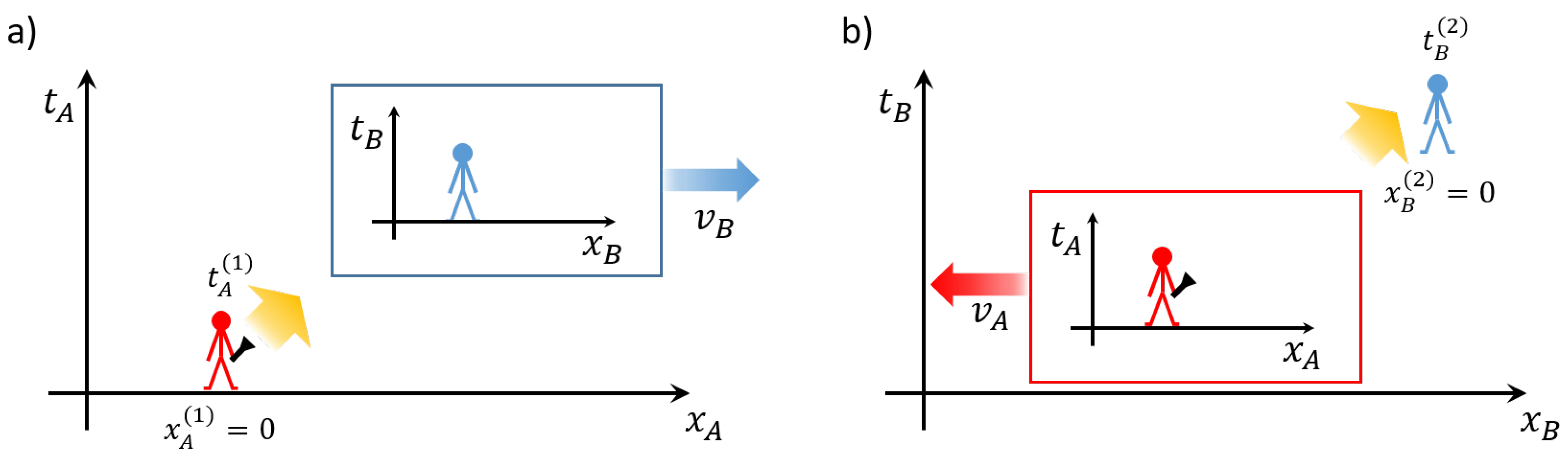
Figure 2.
The spacetime diagram for the propagation of a short light pulse transmitted from Alice to Bob from Alice’s (left) and from Bob’s (right) points of view. Alice’s world line is coloured red and Bob’s is coloured blue. The light pulse (shown in yellow) is transmitted by Alice from point (1) and received by Bob at point (2).
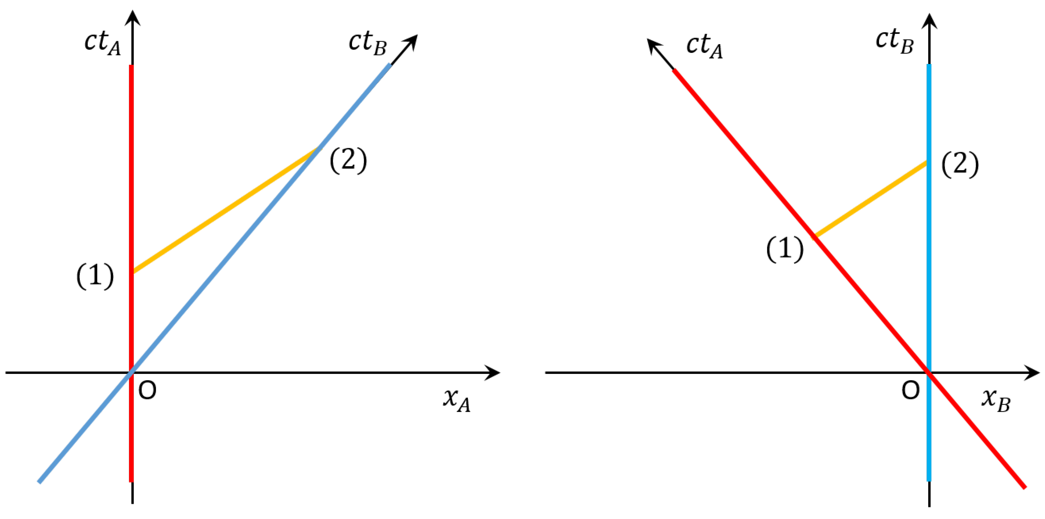
Figure 3.
Both figures show the same thin “box” (or volume) in the spacetime diagram of Bob (a) and of Alice (b). In Bob’s reference frame, the edge of the “box” is parallel to the axis and its length is given by . From Alice’s point of view, the “box” appears deformed to ensure that any spacetime point in Bob’s volume is also in Alice’s volume. The figures moreover show the propagation of light through both spacetime volumes. The light carries a conserved and invariant energy flux . Due to the relativistic deformation of the volume in Alice’s case, the total energy flux crossing the edge of the volume is different from the energy flux crossing the edge. Consequently, Alice and Bob measure different energies at fixed times even when observing the same wave packet of light.
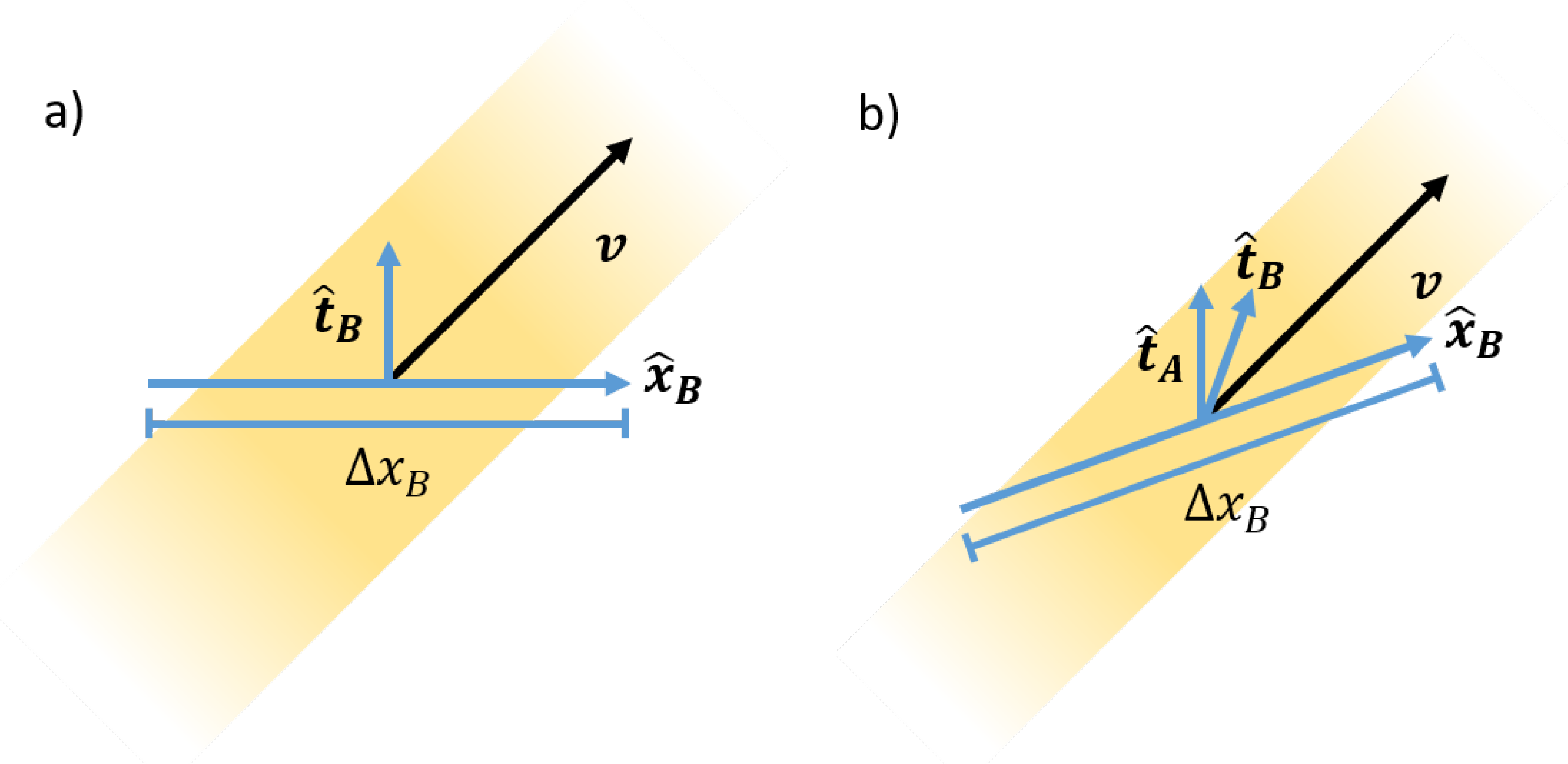
Figure 4.
The diagram shows the contribution of right-propagating blips to the field observables measured by Alice at the origin. From one point of view, blips distributed along the axis (solid red) contribute non-locally to the field observable. As blips at one point in spacetime can be identified with blips at all points along their world-lines (marked in yellow), blips distributed along axis (hollow red) provide an equivalent contribution to the field observables as blips along the axis on the same world-line.
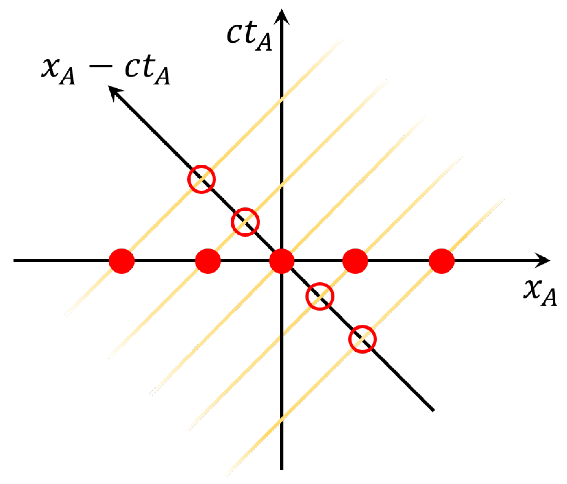
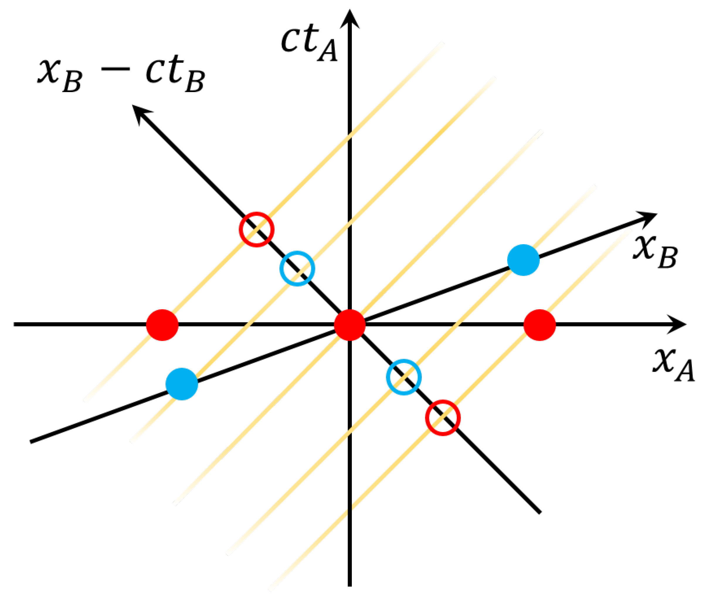
Figure 5.
The diagram shows the contribution of right-propagating blips to Alice’s and Bob’s field observables at the origin. Blips distributed along the axis (solid red) and along the axis (solid blue) contribute equally to Alice’s and Bob’s field observables respectively. As blips at one point in spacetime can be identified with blips at all points along their world-lines (marked in yellow), blips distributed for example along the axis (hollows in red and blue) provide an equivalent contribution to Alice’s and Bob’s field observables as blips along the axis and axis on the same world-line.
Disclaimer/Publisher’s Note: The statements, opinions and data contained in all publications are solely those of the individual author(s) and contributor(s) and not of MDPI and/or the editor(s). MDPI and/or the editor(s) disclaim responsibility for any injury to people or property resulting from any ideas, methods, instructions or products referred to in the content. |
© 2024 by the authors. Licensee MDPI, Basel, Switzerland. This article is an open access article distributed under the terms and conditions of the Creative Commons Attribution (CC BY) license (http://creativecommons.org/licenses/by/4.0/).
Copyright: This open access article is published under a Creative Commons CC BY 4.0 license, which permit the free download, distribution, and reuse, provided that the author and preprint are cited in any reuse.


