

Submitted:
01 January 2024
Posted:
03 January 2024
You are already at the latest version
Abstract
In this paper, we present a three-step sixth-order iterative schemes to estimate the solutions of a nonlinear systems of equations, for predicting the shear strength of a reinforced concrete beam. This procedure is designed by means of a weight function technique. The values for the parameters of this system were randomly selected inside the prescribed ranges by technical standards for structural concrete; moreover, some of this parameters were fixed taking into consideration the solvability region of the adopted steel constitutive model. The efficiency of the new class is compared with other current schemes, with very good results.
Keywords:
Nonlinear systems
; iterative methods
; reinforced concrete
; shear behaviour
; stability
; convergence order
; efficiency
1. Introduction
Reinforced and prestressed concrete beams represent a structural type that resists internal stresses in a relatively complex manner due to their constitutive nature. Prior to cracking of the concrete, the shear loads are carried by a set of diagonal compressive stresses complemented by another set of diagonal tensile stresses acting perpendicular to the first ones. Once the concrete tensile strength is reached, cracks form in the direction normal to the diagonal tensile stresses while preexisting cracks spread and change inclination. Then the ability of concrete to transmit diagonal tensile stresses is significantly reduced and the appropriate reinforcement is necessary to create a new system of internal stresses that carry the shear acting on the beam after cracking. Shear design procedures for reinforced concrete that determine the inclination of such cracks by considering the strains in the diagonally stressed concrete, as well as in the longitudinal and transverse reinforcement, are known as Compression Field Theories (CFT) [1,2].
As justified at Section 2, CFT mechanical models involve several types of nonlinearities, among other reasons, due to the constitutive relationships of the reinforced concrete. The implementation of these models usually requires the application of numerical methods for solving the corresponding nonlinear equations, such as, for example, Newton-type methods [3]. In fact, the correct solver for solving a nonlinear problem is often a choice between computational cost and accuracy [4,5,6,7]. Moreover, in this work the previous determination of a solvability region using algebraic procedures is also necessary in order to improve the efficiency of the numerical solver, as indicated at Section 2.
Solving systems of nonlinear equations is an important problem in science and engineering. The objective is to find the roots of the nonlinear system , being F a multidimensional function, , on D convex set , of size , , being , , the functional coordinates of F.
One of the most commonly used methods, is the classical Newton method, which has a quadratic order of convergence and iterative expression
where is a Jacobian matrix of F at k-th iteration.
Several Newton type procedures, by using different techniques, have been published in the last years. Their main aim is accelerating the convergence or increasing their efficiency. In the last section we are going to recall some of them, for comparison purposes.
All the schemes we are going to mention use, in their iterative expression, the Jacobian matrix of function F and have, under the usual conditions, convergence order 6. We will compare these methods, from the point of view of results, convergence order and computational efficiency, with the methods proposed in this paper that also have order 6 and use in their expressions.
In [8], by using the weight function procedure, the authors designed a Jarratt-type method for solving nonlinear systems, denoted by , whose iterative expression is:
where I denotes the identity matrix of size . This method needs to evaluate the Jacobian matrix in two points and uses two inverse operators. These elements increase the number of operations per iteration.
In order to reduce the number of inverse operators, Narang et al. in [9] from a Chebyshev-Halley-type family, constructed a class of iterative schemes of sixth-order, one of its members denoted by has the following iterative expression:
where and .
Behl et al. in [10], using the indeterminate parameter procedure, designed a family of iterative sixth-order methods for solving systems of nonlinear equations, one of whose members, denoted by PM1, has the iterative expression
Finally, Yaseen and Zafar presented in [11] a Jarratt-type scheme of three-steps for solving nonlinear systems, denoted by , with sixth-order convergence and iterative expression
where and .
2. Problem Statement
In [1], the authors proposed this stress-strain relationship for concrete cracked in tension:
where represents the contribution of tensile stresses in the concrete between the cracks or tension stiffening effect, is the principal tensile strain, being the modulus of elasticity of the concrete, the strain related to the strength of the tensile, . Coefficient is equal to 1.0 in case of fast and non-cyclic loads and for deformed bars.
Regarding to the concrete behaviour in compression, Vecchio and Collins formulated in [12], inside the Modified Compression Field Theory (MCFT), the following relationship between diagonal compressive strain, and the diagonal (or principal) compressive stress, :
where is the compressive strain related to the compressive strength of concrete in a cylinder test , is the coexisting principal tensile strain, and is the maximum compressive stress in a diagonally cracked web.
In CFT procedures, perfect bond between concrete and steel is assumed; in consequence, any deformation developed by the reinforcement is identical to the one experienced by the surrounding concrete in the same direction; thus, a single average strain tensor of the composite material is adopted. The following relationship is considered by compatibility of the strains in the reinforcement and the diagonally stressed concrete:
where is the mean longitudinal strain and is the mean transversal strain on the web of a beam oriented according to the orthogonal directions (see Figure 1). The strain is aligned in the direction of the compressive struts, at angle to the longitudinal axis (x) of the beam. Moreover, due to strain tensor, the main tensile strain is
On the other hand, in CFT models the equilibrium between the external loads and the internal forces is governed by the following equations:
where is the angle of the main tensile stress, z is the flexural lever arm, s is the stirrup spacing, is the internal shear force, and is the web width; , and are the cross-section surfaces for the longitudinal bars, the stirrup legs and the prestressed reinforcement, respectively, and , and are the related mean tensile stresses. The angles of inclination of principal strains coincide with the angles of inclination of principal stresses; this is known as EPA assumption or as Wagner’s hypothesis [2,13].
The main difference among CFT methods lies in the treatment of the steel behavior [12,14,15]. In this work one of the most recent approaches to the steel behaviour is adopted, the so-called Refined Compression Field Theory (RCFT) [15,16], which is based on the concept of an embedded bar model that takes into account the concrete tension stiffening effect between cracks. This last theory allows us to implement, in the most general case, the following average stress-strain model for each kind of steel reinforcement in the beam (that is, the transverse stirrups and the longitudinal reinforcement):
where the subscripts x and t refer to the longitudinal and the transverse reinforcement, respectively (then, expression (13) actually involves two equations); is the steel yield stress, is the elastic modulus of the steel, is the average tensile stress in the steel, is the average strain in the reinforcing bar, is the apparent yield strain (cf. [15]), is the cross-section of the longitudinal or transverse steel bars, M is the bond parameter and is the area of concrete bonded to the bar playing in the tension stiffening effect (that usually is considered equal to the rectangular surface around the bar and on a distance not exceeding 7.5 from its center, where is the diameter of the bar).
In case of prestressed concrete elements, the following two more equations are needed:
where Equation (14) represents the strain compatibility, being and the strain by imposition of the prestressing system and the strain of the prestressing strand, respectively, and Equation (15) represents the stress-strain relation for the prestressing steel, being and its yield stress and elastic modulus, respectively.
In summary, for a given value of tensile principal strain in concrete, , where such strain works as an input parameter, the shear model for the prediction of the load-deformation behavior of a prestressed concrete beam is based on the nonlinear system of Equations (3-11), with to 10 equations (notice that Equation (13) is actually two equations in turn) in the 10 unknowns (, , , , , , , , and ).
Equation (13) is based on the concept of forces balance between a general section (or non-cracked section, where both steel and the surrounding concrete contribute) and a cracked section (where only the reinforcement resist the internal forces; see Figure 2). The greatest value of the area in order to preserve the solvability of the embedded steel constitutive model proposed by the RCFT (i.e., to preserve the internal equilibrium of forces, so that as the concrete participation increases, the steel tension decreases) is obtained by applying the following coefficient [17]:
where the coefficient represents the boundary of the solvability region for the embedded steel constitutive model and is the strain corresponding to the steel yield stress (i.e. ). For certain design cases, the previous boundary may lay within the design range prescribed by technical codes for the tension stiffening area, .
3. Development and Convergence of the Method
By using the weight matrix function procedure we present a class a three-step iterative methods with the following iterative expression:
where is the variable of the weight function G, and b, i, and h free parameters.
On the other hand, since F is a sufficiently differentiable Fréchet function, we can regard in a neighbourhood of . Using Taylor developments and being nonsingular,
where , for . Also, , as and . Therefore,
being . For more details of this notation we can see [18].
Indeed, following the terms introduced by Artidiello et al. in [19], a matrix function can be defined in such a way that its Fréchet derivatives holds
- (a)
- being ,
- (b)
- being ,
when is the Banach space of real matrices.
In the next result, we present the convergence of family (17).
Theorem 1.
Let us be a sufficiently Fréchet differentiable function defined on an open neighborhood D of , a zero of F. Let also be a sufficiently differentiable matrix function. Suppose that is nonsingular, and that is a seed sufficiently close to ξ. Therefore, the sequence from (17) converges to ξ with order of convergence six if , , , , and , being and I the identity matrix of size . In this case, the error equation is
where and ,
Proof.
By means of the Taylor expansion of and about , we get
and
We can deduce that
where , , and
Then,
and
Moreover,
So,
and
For the weight function G,
that is
We denote . So its Taylor development can be expressed as:
So,
and
Now, we denoted . So its Taylor expansion is:
If , then
Therefore, the error equation is:
Fixing , , , and , the error equation becomes
With this the proof is finished. □
4. Efficiency Indices
To compare the iterative methods used, we will use the efficiency index , introduced by Ostrowski [20], being the convergence order and d is the amount of functional evaluations, per iteration. Let us also remark that it is necessary to evaluate n scalar functions for each F and for each .
Another index for comparing different iterative schemes was introduced in [21]
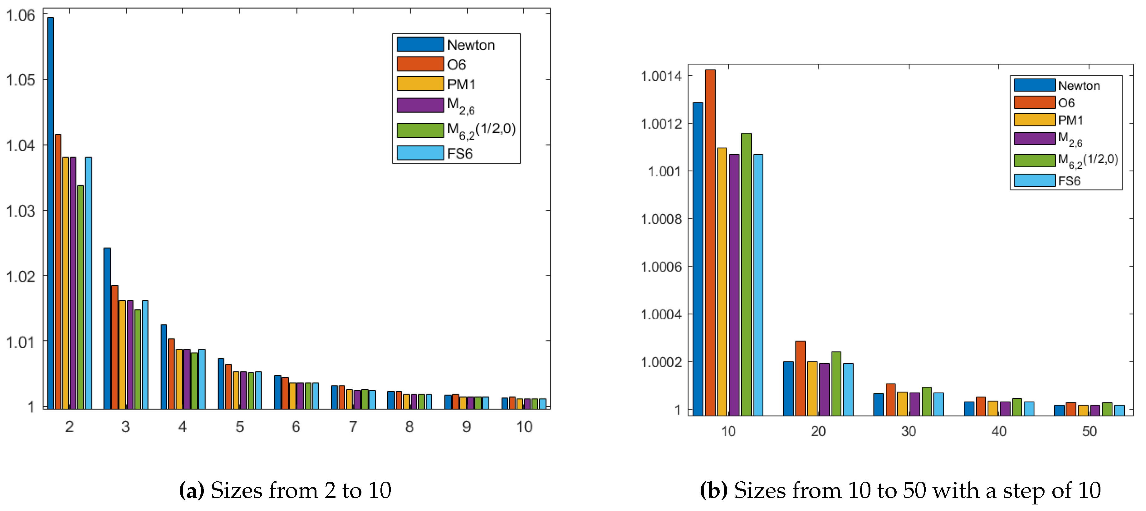
In the Figure 3 we compare the computational efficiency index, , of several methods with Newton’s method.
where is the number of products/quotients per iteration.
In each iteration five linear systems are solved with the same coefficient matrix, there are two matrix-vector products and, with respect to functional evaluations, we have two evaluations of Jacobian matrices and three of functions. The computational cost of method O6 is

Table 1.
Comparisons of CE.
| Method | CE |
|---|---|
| Newton | |
| O6 | |
| PM1 | |
| FS6 |
The results are represented in semi-logarithmic scale, see Figure 3, for a better visualization of the differences between the indices (CI), for the methods used and several sizes of the systems.
5. Numerical Performance
We analyse the performance of the methods described above, to check their efficiency and compare it with other known methods The results from Table 2 to Table 5 correspond to the calculations made with Matlab , by using variable precision arithmetics with 1200 digits of mantissa, on a PC equipped with a Core™ i5-5200U CPU 2.20GHz. In all the tables we show the residuals and of the last iteration satisfying the stopping criterium or being lower than . Moreover, a computational estimation of the order of convergence is obtained by means of ACOC introduced in [22] as
5.1. Example
We consider the nonlinear system [23]:
with seed , being in this case, .
In Table 2, it can be observed that the number of iterations of all the sixth-order schemes are equal and the time is very similar in all of the methods; however, the best residual is obtained by the proposed scheme O6. The ACOC estimates the theoretical order of convergence accurately, in all cases.
Table 2.
Numerical results for Example 5.1.
| Method | Iteration | e-Time | |||
|---|---|---|---|---|---|
| Newton | 8 | 2.0 | 0.98 | ||
| O6 | 4 | 0.0 | 6.0 | 0.99 | |
| FS6 | 4 | 6.0 | 1.02 | ||
| PM1 | 4 | 6.0 | 0.99 | ||
| 4 | 5.0 | 1.00 | |||
| 4 | 6.0 | 1.02 |
5.2. Example
The second example is given by [24]
with seed and .
Table 3.
Numerical results for Example 5.2.
| Method | Iterations | e-Time (sec) | |||
|---|---|---|---|---|---|
| Newton | 11 | 2.0 | 9.99 | ||
| O6 | 5 | 6.0 | 10.24 | ||
| FS6 | 5 | 6.0 | 11.00 | ||
| PM1 | 6 | 6.0 | 10.58 | ||
| 6 | 6.0 | 11.07 | |||
| 6 | 6.0 | 10.79 |
5.3. Example
Let us define now the nonlinear system [24],
with seed , and .
Table 4.
Numerical results for Example 5.3.
| Method | Iterations | e-Time (sec) | |||
|---|---|---|---|---|---|
| Newton | 10 | 2.0 | 1.22 | ||
| O6 | 5 | 6.0 | 1.24 | ||
| FS6 | 4 | 6.0 | 1.20 | ||
| PM1 | 5 | 6.0 | 1.27 | ||
| 5 | 5.0 | 1.39 | |||
| 5 | 6.0 | 1.39 |
Let us notice in Table 4 that O6 and FS6 provide a solution satisfying the stopping criterium in less iterations as the rest of schemes. This is the reason why their residuals are not as close to zero as those of other schemes. The e-time of O6 is the second best-one.
Regarding the applied problem described in Section 2, the nonlinear shear model of a reinforced concrete beam, as its underlying data are provided by random values with few digits inside the prescribed ranges by technical standards for structural concrete; moreover, some of this parameters were fixed taking into consideration the solvability region of the adopted steel constitutive model. The stopping criterium is or being lower than . The results provided by the new and existing schemes appear in Table 5. The ACOC does not appear in this table, as it yields to unstable data in all cases.
Table 5.
Problem statement Section 2.
Table 5.
Problem statement Section 2.
| Method | Iterations | e-Time (sec) | ||
|---|---|---|---|---|
| Newton | 5 | 0.0342 | 18.3242 | |
| O6 | 3 | 9.0862 | 21.6703 | |
| FS6 | 3 | 218.18 | 22.1258 | |
| PM1 | 4 | 3.8554 | 21.9594 | |
| 4 | 7.3926 | 28.0727 | ||
| 3 | 0.0423 | 22.4797 |
However, the best methods in terms of number of iteration are O6, FS6 and , all with 3 iterations. Among them, the lowest e-time corresponds to our proposed scheme O6. This good performance allows us to assure the reliance and robustness of our proposed procedure.
6. Conclusions
In this article, we have developed a vectorial parametric family of numerical methods of order six, to solve a constitutive equation of reinforced concrete (6). The new class (O6) is compared to other existing methods with the same order of convergence and also with Newton’s scheme. All the comparison procedures need the same or more, iterations and achieve lower precision results in the same or lower execution time, to achieve the required tolerance. This proves the accuracy, robustness and applicability of the proposed scheme.
Author Contributions
Conceptualization, , J.J.P. ; methodology, F.I.C..; software, A.C. and F.I.C.; formal analysis, J.R.T.; investigation, A.C. ; writing—original draft preparation, J.J.P. and A.M.H.; writing—review and editing, A.C. and J.R.T. All authors have read and agreed to the published version of the manuscript.
Funding
No funding.
Institutional Review Board Statement
Not applicable.
Informed Consent Statement
Not applicable.
Data Availability Statement
Not applicable.
Conflicts of Interest
The authors declare no conflict of interest.
References
- Collins, M.P.; Mitchell, D. Prestressed concrete structures; Vol. 9, Prentice Hall Englewood Cliffs, NJ, 1991.
- on Shear, A.A.C..; Torsion. Recent approaches to shear design of structural concrete. Journal of structural engineering 1998, 124, 1375–1417.
- Galántai, A. The theory of Newton’s method. Journal of Computational and Applied Mathematics 2000, 124, 25–44. [Google Scholar] [CrossRef]
- Hernández-Díaz, A.M.; Bueno-Crespo, A.; Pérez-Aracil, J.; Cecilia, J.M. Multi-objective optimal design of submerged arches using extreme learning machine and evolutionary algorithms. Applied Soft Computing 2018, 71, 826–834. [Google Scholar] [CrossRef]
- A.M. Hernández-Díaz, A. Muñoz, J.J.A.; Sáez, A. Buckling design of submerged arches via shape parameterization. Computational and Mathematical Methods 2019, 1, e1057.
- J.F. Jiménez-Alonso, J. Pérez-Aracil, A.H.D.; Sáez, A. Effect of Vinyl flooring on the modal properties of a steel footbridge. Applied Sciences 2019, 9, 1374. [CrossRef]
- J. Pérez-Aracil, C. Camacho-Gómez, A.H.D.; E. Pereira, D.C.; Salcedo-Sanz, S. Memetic coral reefs optimization algorithms for optimal geometrical design of submerged arches. Swarm and Evolutionary Computation 2021, 67, 100958. [CrossRef]
- Hueso, J.L.; Martínez, E.; Teruel, C. Convergence, efficiency and dynamics of new fourth and sixth order families of iterative methods for nonlinear systems. Journal of Computational and Applied Mathematics 2015, 275, 412–420. [Google Scholar] [CrossRef]
- Narang, M.; Bhatia, S.; Kanwar, V. New two-parameter Chebyshev–Halley-like family of fourth and sixth-order methods for systems of nonlinear equations. Applied Mathematics and Computation 2016, 275, 394–403. [Google Scholar] [CrossRef]
- Behl, R.; Maroju, P.; Motsa, S. Efficient family of sixth-order methods for nonlinear models with its dynamics. International Journal of Computational Methods 2019, 16, 1840008. [Google Scholar] [CrossRef]
- Yaseen, S.; Zafar, F. A new sixth-order Jarratt-type iterative method for systems of nonlinear equations. Arabian Journal of Mathematics 2022, 11, 585–599. [Google Scholar] [CrossRef]
- Vecchio, F.J.; Collins, M.P. The modified compression-field theory for reinforced concrete elements subjected to shear. ACI J. 1986, 83, 219–231. [Google Scholar]
- Hernández-Dı, A.; Gil-Martı, L.; others. Analysis of the equal principal angles assumption in the shear design of reinforced concrete members. Engineering structures 2012, 42, 95–105. [Google Scholar] [CrossRef]
- Belarbi, A.; Hsu, T. Constitutive laws of concrete in tension and reinforcing bars stiffened by concrete. Structural Journal 1994, 91, 465–474. [Google Scholar]
- L. M. Gil-Martín, L. María, E.H.M.; Aschheim, M.; Pantazopoulou, S. Refinements to compression field theory, with application to wall-type structures. American Concrete Institute Special Publication 2009, 265, 123–142. [Google Scholar]
- M. Palermo, L.M. Gil-Martin, E.H.M.; Aschheim, M. Refined compression field theory for plastered straw bale walls. Construction and Building Materials 2014, 58, 101–110. [CrossRef]
- A. M.Hernández-Díaz.; García-Román, M. Computing the refined compression field theory. International Journal of Concrete Structures and Materials 2016, 10, 143–147. [CrossRef]
- Cordero, A.; Hueso, J.L.; Martínez, E.; Torregrosa, J.R. A modified Newton-Jarratt’s composition. Numer. Algor. 2010, 55, 87–99. [Google Scholar] [CrossRef]
- Artidiello, S.; Cordero, A.; Torregrosa, J.R.; Vassileva, M.P. Multidimensional generalization of iterative methods for solving nonlinear problems by means of weight-function procedure. Applied Mathematics and Computation 2015, 268, 1064–1071. [Google Scholar] [CrossRef]
- A.M., O. Solutions of equations and systems of equations; Academic Press: New York, 1966. [Google Scholar]
- Cordero, A.; Torregrosa, J.R. On interpolation variants of Newton’s method for functions of several variables. Journal of Computational and Applied Mathematics 2010, 234, 34–43. [Google Scholar] [CrossRef]
- Cordero, A.; Torregrosa, J. Variants of Newton’s method using fifth-order quadrature formulas. Applied Mathematics and Computation 2007, 190, 686–698. [Google Scholar] [CrossRef]
- Artidiello, S.; Cordero, A.; Torregrosa, J.R.; Vassileva, M.P. Design and multidimensional extension of iterative methods for solving nonlinear problems. Applied Mathematics and Computation 2017, 293, 194–203. [Google Scholar] [CrossRef]
- Cordero, A.; Jordán, C.; Sanabria, E.; Torregrosa, J.R. A new class of iterative processes for solving nonlinear systems by using one divided differences operator. Mathematics 2019, 7, 776. [Google Scholar] [CrossRef]
Figure 1.
Strain compatibility between diagonally stressed concrete and the reinforcement in the cracked web of a reinforced concrete beam.
Figure 1.
Strain compatibility between diagonally stressed concrete and the reinforcement in the cracked web of a reinforced concrete beam.
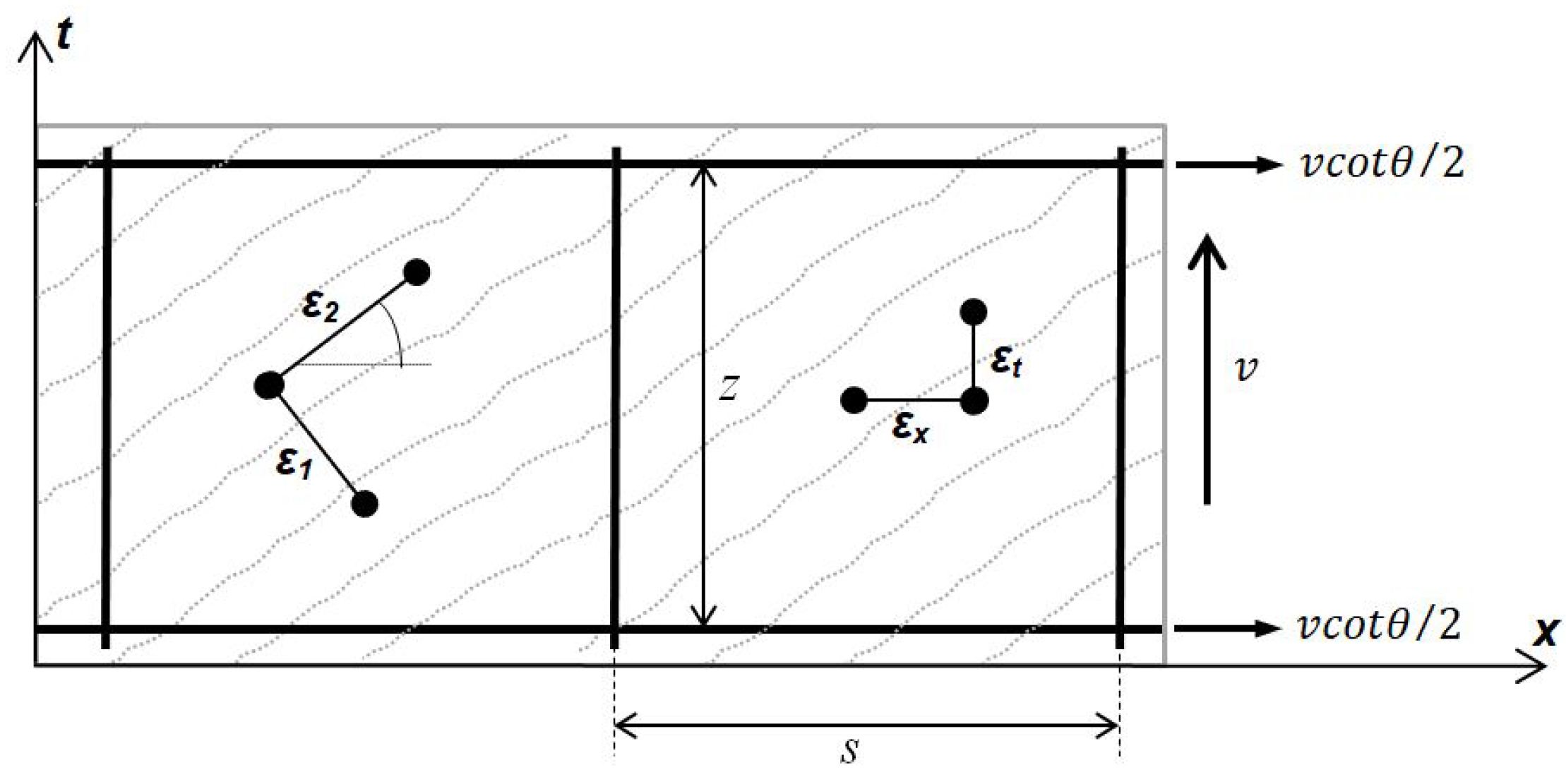
Figure 2.
Average stresses profiles ( and ) for an embedded reinforcement constitutive model including several cracks.
Figure 2.
Average stresses profiles ( and ) for an embedded reinforcement constitutive model including several cracks.
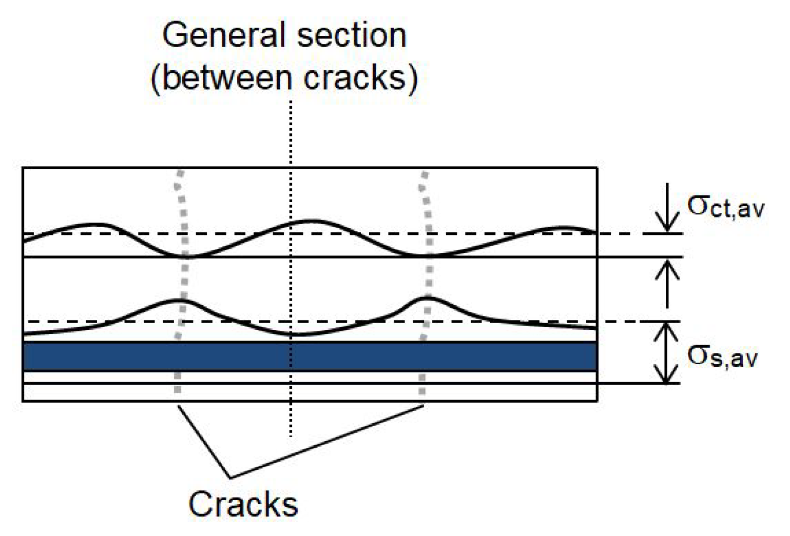
Figure 3.
Computational Efficiency Indices.
Disclaimer/Publisher’s Note: The statements, opinions and data contained in all publications are solely those of the individual author(s) and contributor(s) and not of MDPI and/or the editor(s). MDPI and/or the editor(s) disclaim responsibility for any injury to people or property resulting from any ideas, methods, instructions or products referred to in the content. |
© 2024 by the authors. Licensee MDPI, Basel, Switzerland. This article is an open access article distributed under the terms and conditions of the Creative Commons Attribution (CC BY) license (http://creativecommons.org/licenses/by/4.0/).
Copyright: This open access article is published under a Creative Commons CC BY 4.0 license, which permit the free download, distribution, and reuse, provided that the author and preprint are cited in any reuse.