
Submitted:
31 December 2023
Posted:
03 January 2024
You are already at the latest version
Abstract
There is a growing concern about climate change being a serious threat to insurance business sustainability. Knowing if climate warming is a cause for claims and losses increase, and how this cause-effect relationship will develop in the future are two open major questions. In this article, we answer both questions by particularizing the geographical area of Spain, and a precise risk, hailstorm in crop insurance in the line of business of wine grapes. We measure climate change thanks to the Spanish Actuarial Climate Index (SACI). We use a database containing all the claims caused by hail risk in Spain from 1990 to 2022. With homogenized data, we consider as dependent variables the monthly number of claims, monthly number of loss costs equal to one, and monthly total losses. The independent variable is the monthly Spanish Actuarial Climate Index (SACI). We try to explain the former through the latter using regression and quantile regression models. Our main finding is that climate change as measured by SACI explains these three dependent variables. We also give an estimation of the increase of the monthly total losses Value at Risk, corresponding to a future increase in climate change measured in units of SACI. Spanish crop insurance managers should carefully incorporate these conclusions into their decision-making process to keep this line of business sustainable in the future.
Keywords:
Climate change
; Crop insurance
; Hail risk
; Quantile regression
; Regression (List three to ten pertinent keywords specific to the article
; yet reasonably common within the subject discipline.)
1. Introduction
According to the United Nations Climate Action Forum, Climate change refers to long-term shifts in temperatures and weather patterns. Such shifts can be natural, due to changes in the sun’s activity or large volcanic eruptions. But since the 1800s, human activities have been the main driver of climate change, primarily due to the burning of fossil fuels like coal, oil and gas. Burning fossil fuels generates greenhouse gas emissions that act like a blanket wrapped around the Earth, trapping the sun’s heat and raising temperatures [1]. This process is a long-term one, affecting human beings in many instances as their lives, properties, transportation infrastructures, etc (see for instance [2,3,4]). As the insurance business spreads through all aspects of economic and individual human life giving protection against all sorts of claims, substituting random losses by sure indemnities, the question of how climate change is affecting the insurance business has arisen as a critical one for its present management and future sustainability.
During the last years, many extremal events like fires, floods, droughts, storms, and pandemics have negatively affected the balance sheet of insurance companies to the point of motivating their retreat from some lines of business in some geographical areas where the losses have increased to unaffordable bounds (see for instance [5]). In the scientific world, the concern about insurance business sustainability has mobilized lots of efforts to try to understand how insurance companies should include climate change effects in their medium and long terms management (see [6,7,8,9,10]). The efforts to technically cope with the new situation, imply advanced Statistical and Data Science methodologies (see for instance [11,12,13,14]). General insurance principles like risk insurability, pooling, and diversification in a new context of climate shift are also under discussion ([15]). Insurance areas analyzed from the point of view of climate change are those related to mortality and property losses (see for instance [11,13,14]). Also, an important field of research is that of agricultural insurance ([16,17]) where our paper is located. In crop insurance, all the weather-related extreme events are relevant and may be influenced by climate change.
This paper focuses on hailstorm risk in the line of business of Spanish wine grapes. This is a daunting risk for insurance managers because of its variability in time and space and also because its events are rather local and ubiquitous. Hail risk in agricultural insurance is analyzed for instance in [18,19,20]. Hailstorms are very harmful for crops yet their evolution under global warming has rarely been a subject of study. The paper [21] studies its influence in the conditions (moisture, convective instability) under which the hailstones get generated, giving a geographical sketch of hailstorm future frequency evolution. One particular conclusion is that it may rise in Europe as anthropomorphic warming grows. The work [22] applies Tobit regressions to conclude that a strong positive relation exists between hailstorm activity and hailstorm damage, as predicted by minimum temperatures using simple correlations. This relation suggests that hailstorm damage may increase in the future if global warming leads to a further temperature increase. Finally, [23] finds a strong influence of climate change, as measured by Convective Available Potential Energy (CAPE) and also by totals–totals index (TT index), on the frequency and intensity of hail events in several locations around southeastern Australia. They use reanalysis data (a data set comprising a blend of observations and model simulations) and direct data obtained from the Australian National Climate Centre.
We aim to investigate if climate change has any influence on hailstorm risk in Spanish wine grapes, a rather important line of business in agricultural insurance given that Spain has the largest wine grapes cultivated area among European countries ([24]). According to our model results, we conclude that climate change explains the increase in the monthly number of claims, monthly number of loss costs equal to one, and monthly total losses observed from 1990 to 2022.
2. Materials and Methods
2.1. The Database on Hail Risk in Spanish Wine Grapes
The database on wine grape hailstorm claims is sourced from Agroseguro, the Spanish coinsurance pool of agricultural insurance grouping seventeen insurance companies. Agroseguro manages the risks and policies on behalf of those companies and participates in the Spanish system of agricultural insurance together with the Spanish State, and professional agricultural associations and cooperatives. During the year 2022, its wine grapes line of business has insured 46.44% of the total of cultivated surface, and the total value of the production (total insured sum) has been €(see [25]).
The database has records from 1990 to 2022. It contains information on 49 provinces and 240 regions with 893,144 yearly policies. There have been 692,733 claims during the 33 years and some relevant yearly figures are given in Table 1. Figure 1 visually depicts the evolution of both the number of plots and hailstorm claims over the specified period. Therefore, this database provides a thorough view of hailstorm risk in the Spanish wine grapes line of business from 1990 to 2022. The column Crop Yield in Table 1 is calculated from the individual plots information contained in the database, and it refers to the expected potential production that could be obtained in each insured plot based on its normal edaphic, climatic, planting, sowing, and cultivation conditions.
Claim data have also been monthly aggregated and months free of claims have been filled with zeros, see the blank spaces in Table 2. This allows for a nuanced understanding of seasonal patterns and trends over the years. This is important for studying the impact of climate change because one key element is to know the relevant season for hailstorms, which will be later defined as a sequence of months.
2.1.1. The Normalized Number of Claims, N.
We normalize the number (yearly or monthly) of claims by dividing it by the number of plots of that year. In other words, we calculate the proportion of policies on which claims occurred compared to the total number of plots of that year (see Table 2 for monthly figures).
The plot of normalized yearly claims is depicted in Figure 2. It illustrates the true yearly trend in the number of hailstorm claims in the Spanish wine grape line of business from 1990 to 2022, taking into account the growth in the number of plots. We observe quite a jagged shape showing significant variation in the yearly number of claims, reflecting the high uncertainty and variability of hailstorm risk. Anyway, its upward trend indicates an increase in the frequency of the normalized number of hailstorm events that we wish to explain through climate warming.
Figure 3 shows the trend in the number of monthly hailstorm claims from January 1990 to December 2022. The data are normalized to more accurately show the relative changes in the number of claims from month to month.
In addition, in Table 2 and Figure 3 we observe an important and clear seasonal pattern, that is, the vast majority of hail claims happen from April to September, which is related either to the weather conditions that produce hailstorms and the growth cycle of wine grapes. This is indeed an important conclusion that allows us to choose the period going from April to September as the hailstorm season that will be later used in our models aiming to explain the insurance claims and losses by climate change.
2.1.2. The normalized Number of Loss Costs Equal to One, .
The loss cost is the ratio of severity over insured capital and is a simple and direct way of assessing the degree of damage caused by a claim. From now on, let us note for the monthly number of loss costs equal to one (if monthly or yearly will be clear from the context). means that this number of losses equals the insured capitals, thus indicating the maximum degree of burden for the insurance company in those claims. In Figure 4 we plot the yearly normalized as a percentage of the yearly number of claims. Although the rate is low in most years, there are still several spikes, indicating that hailstorms caused serious economic losses in specific years. Overall, the least squares line is increasing, indicating an increasing tendency of the maximum damages over time. We aim to explain this long-term increase through climate change.
2.1.3. The Homogenized Losses, L.
Over time, factors such as inflation increases in the number of policies and/or cultivated surfaces, and rising productivity levels may influence insurance losses. As a result, claims of similar intensity at different dates may result in larger losses than in previous years. Therefore, implementing a homogenization process becomes crucial when analyzing insurance losses over time. This homogenization allows more accurate and fair comparisons across time, thereby facilitating a thorough understanding of the changing impacts of insurance claims and their economic consequences(see [22,26,27]).
In our research, we use a specific normalization formula to analyze hailstorm losses. This formula allows us to effectively compare loss data across different years, even in changing market conditions and agricultural productivity. The formula for normalized insurance loss is:
where represents the total insurance losses ,where , and . The is a specially designed index that accounts for annual changes in insurance capital and crop yields since 1990. The calculation method for the insurance value index is as follows:
This index is an annual time series that comprehensively accounts for changes in total insurance capital and crop yields since 1990. Specifically, the index reflects the relative changes in annual insurance capital compared to the baseline level in 1990. It also incorporates the yearly variations in crop yield to reflect fluctuations in agricultural production and market conditions. Through this approach, our insurance value index effectively homogenizes hailstorm loss data across different years, allowing fair and consistent comparisons among different dates. Thus, even amidst changes in market conditions and agricultural productivity, we can accurately measure and analyze the trends and impacts of hailstorm losses. From here after we will always work with homogenized losses, even when we shortly name them losses.
Considering the logarithm of the insurance losses is motivated by two key factors. Firstly, this transformation helps in moderating the impact of outliers on the model by reducing the data dispersion, contributing to a more robust model. Secondly, the logarithmic transformation stabilizes the variance structure of the data, thereby enhancing the accuracy of the regression (see [30]). From Figure 5, we can see that the logarithmic losses are more stable than the original ones. Note that we only take the logarithm of the data for months with claims, while we still record with zeroes the months with no claims.
We can further analyze the total loss variable by considering its yearly figures in Figure 6, where three of its yearly quantiles (90th, 95th, and 99th) are plotted, showing increasing trends over time in all three cases. This growth seems to support the idea that climate change influence might still be significant for higher probability levels, not only for means. We aim to test this hypothesis later. Let us finally comment that, if the frequency and severity of hailstorm extreme events continued to increase over time, this could finally affect the business sustainability, to what extent though? Would it be possible to quantify this effect? We try to answer this question later.
2.2. The Spanish Actuarial Climate Index (SACI)
Until now we have presented and explained the data referred to the dependent variables: the normalized monthly number of claims N, the normalized number of loss costs equal to one , and the homogenized monthly total losses L. We now turn to the other side where we aim to use as the independent variable an index of climate change.
To help insurance companies measure and manage climate risk, actuaries in North America have defined the Actuaries Climate Index™ (ACI), which combines information from several important weather variables from the historical records of the United States and Canada. The ACI divides the main geographical area (USA and Canada) into a grid of cells corresponding to a resolution and then collects in each cell data from the relevant historical meteorological variables to calculate the six ACI components: days of warm temperature (), days of cool temperature (), precipitation (P ), drought (D ), wind speed (W ) and sea level (S). For each cell, ACI uses the reference period from 1961 to 1990 where mean and standard deviations are calculated for all the components, and these are posteriorly normalized by these figures, so their variations are measured in units of the corresponding reference period standard deviation. Then it calculates the mean of the six normalized components to obtain a cell-wise index, although the T10 component is subtracted to obtain a meaningful magnitude:
Finally, the ACI relative to any geographical area contained in the main one is the average of the cell-wise indexes, through the cells covering the area of interest. The ACI can also be particularized to any given season by collecting the data relative to that season and following the same process. In summary, any ACI increase posterior to 1990 will denounce a warming in that area as approximately measured in standard deviation units (see [28]).
The Iberian Actuarial Climate Index (IACI) is the actuarial climate index specific to the Iberian Peninsula, built using the ACI method (see [29]) though with data relative to the Iberian Peninsula taken from the ERA5 Re-Analysis. The ERA5-Land reanalysis data is a high-resolution dataset with a horizontal resolution of 0.1° x 0.1° for each grid cell. It was generated by replaying the land component of the ECMWF ERA5 climate reanalysis. Reanalysis combines model data with observations from various sources, including satellites, weather stations, and ocean buoys (see [29]). For our analysis, we will utilize the Spanish regional monthly index derived from the Iberian Actuarial Climatic Index, SACI, providing a comprehensive understanding of climatic changes in Spain.
Figure 7 depicts the variation in the SACI from April to September for each year between 1961 and 2022. From these subplots, it can be observed that certain months, such as July and August, exhibit a significant upward trend, particularly in recent years. In contrast, other months, like April and May, show relatively stable fluctuations. The graph reveals changes in climatic conditions during the peak season of hail disasters yearly. Notably, the rising trend from April to September may reflect changes in meteorological conditions within these months, possibly in connection with some broader trend of global climate change.
2.3. Methods: Linear and Quantile Regressions
This paper aims to explore the relationship between the Spanish Actuarial Climate Index (SACI) and its components and hailstorm damages to the Spanish wine grapes insurance line of business. We employ both linear regression models ([31]) and quantile regression ([32]) methods to analyze the data. Linear regression is a commonly used technique for estimating the linear association between a dependent variable and one or more independent variables. Its general formula is expressed as follows:
In this formula, Y represents the dependent variable, are the independent variables, is the intercept, are the coefficients, and is the error term.
For quantile regression, the general form is:
Here, denotes the quantile of the conditional distribution of the response variable Y given the design matrix X, and the vector represents the quantile regression coefficients. Linear regression provides insights into the relationship between the SACI and the means of hailstorm claims variables, while quantile regression provides the same for their quantiles.
As told earlier, hailstorm claims for Spanish wine grapes are predominantly reported from April to September, as this period corresponds to the primary occurrence of hail claims. In the subsequent analysis, three independent variables regarding hail claims will be used:
- Monthly normalized number of claims, N.
- Monthly number of loss costs equal to one, .
- Monthly homogenized total losses, L.
In linear regression, can be calculated as:
where is the sum of squares of residuals, and is the total sum of squares. In quantile regression, we will calculate a pseudo for the goodness of fit that is no longer based on Ordinary Least Squares (OLS) calculations but on absolute errors (see [33]), using the R function goodfit().
3. Results
3.1. Monthly Normalized Number of Claims,N
In Table 3 we present the results for three linear regression models designed to investigate if there is any relationship between climate variables like SACI and its components, and the mean of N.
- In model 1we investigate the influence of monthly SACI on the mean of N, finding that this is significant at a level. This indicates that it has a somewhat influence on the number of hail claims. However, its is deficient, indicating that the SACI by itself does not explain well the variations in the mean of N.
In model 2
we introduce the components of the SACI to discern their impact on the mean of N. Notably, the high-temperature days , and sea level are significant, suggesting a potential link between these two SACI components and the mean. However, despite their significance, the overall explanatory power of the model, as indicated by the , remains low. While extreme heat and sea level contribute to the predictive model, there is a need for further variables to enhance the accuracy of the analysis.
- In model 3 we give a try to the formulathat incorporates the months from April to September, encompassing the high-incidence season of hailstorms. Despite the statistical significance observed for precipitation () and wind , with coefficients of opposite signs, the overall explanatory power of the model, as indicated by the R-squared value = 0.5, remains relatively moderate, much better than in the precedent case though. It is noteworthy that the month variables attain statistical significance at the 1 percent level, apart from April whose one is at the 10 percent level. This confirms the seasonal pattern in the occurrence of hail events.
In summary, while the relationship between the mean of N and the SACI seems to be quite fragile (model 1, eq.(7)), we have found some evidence through models 2 (eq. (8)) and 3 (eq. (9)) that some of its components like high-temperature days (), Precipitation (), Wind (), sea level () explain the variation of the mean of N until a certain point. We take note that the wind component is significant in model 3 (eq. (9)) with a negative though, which seems to indicate an opposite effect into N from the other significant components. The season variables Apr. to Sep. are also significant, as expected.
Next, we move to the study of the influence of SACI and its components on the quantiles of N.
For this sake, we begin with model 4:
Results are reported in Table 4.
At the 90th percentile, SACI exhibits a statistically significant positive association with the number of claims ( coefficient = 0.018, p< 0.01). For the 95th percentile, although positive, the association is not significant (coefficient = 0.014, p>0.1); notice also that the confidence interval at 95% lies in both negative and positive halves of the real line. At the 99th percentile, the positive relationship is marginally significant (coefficient = 0.005, p<0.1), but the confidence interval is equally deficient. The 99th and 95th percentiles confidence intervals include both positive and negative values, suggesting a certain degree of uncertainty regarding the precise impact of SACI. The two marginally significant positive coefficients and confidence intervals spanning from slightly negative to positive values indicate that the relationships between SACI and N at those percentiles are not as conclusively positive as observed at the lower 90th percentile, as the inclusion of zero in the intervals suggests the possibility of a null effect or a very modest effect that is not statistically distinguishable from zero.
Also, in Table 4, we observed the pseudo R-squared decreases as the quantile increases in quantile regression. The decrease in pseudo R-squared at higher quantiles indicates that the model explanatory power diminishes for extreme observations, suggesting the presence of additional factors or complexities that contribute to the variability in the upper tail of the distribution.
The scatter plot in Figure 8 illustrates the SACI influence on the quantiles of N, with all the reserves motivated by the information contained in Table 4. The quantile lines correspond to model 4 (eq.10). With due caution, we can see that an increase in SACI causes an increase in all three levels of . It seems also that the higher the probability level the less steep the quantile line.
In model 5 we introduce the months relevant to hail risk
while in model 6 we introduce the SACI components together with the months as independent variables:
Table 5 gives the results for these two quantile regression models. We can check that both SACI and its components except the drought -- significantly impact the normalized number of claims across different quantiles. For the significant variables, confidence intervals lie at one or the other side of the origin. In the cases of they are on the positive side showing their increasing influence on . For this happens on the negative half though, denouncing that an increase of the wind component results in a decrease of the corresponding quantile of N (the same happened in the mean of N, see model 3, eq.(9)). These results indicate that SACI, as a comprehensive climate index, has a substantial impact on the extremes of the number of claims N. The months constituting the hailstorm season are all significant, as was expected. As explained in the previous section, pseudo-R-squared values are calculated following [33]. The values obtained for these six models all exceed 0.5, indicating a not negligible fitting score for all these models.
3.2. Monthly Normalized Number of Loss Costs Equal to One, .
Next, we investigate the relationship between as the dependent variable and SACI and its components as independent ones. Remember that a claim with a loss cost equal to 1 implies that the loss equals the value of the insured capital, indicating the full scale of damage for that claim.
In model 7, we investigate the linear regression with the SACI alone as an independent variable:
while model 8 includes also the months composing hailstorms season:
Results for both models are available in Table 5. Results for model 7 (eq. (13)) indicate that SACI is statistically significant at the 1% level, with a coefficient of 0.0003. However, the R-squared value is extremely low, , denoting that the model explanatory power is very weak.
In model 8 (eq. (14)), we introduce the months as independent variables (April to September). We observe that among the month variables, only May, July, and August are statistically significant. This is a notable difference compared to the case of the number of claims N, which might indicate that not any month in the hailstorm season is relevant to the loss costs being equal to one, only May, July, and August. Overall, the R-squared value of the model increases to 0.146, indicating that the introduction of the month variable has improved its ability to explain the mean of .
In summary, we have found through model 8 (eq. (14)) that the SACI influences to a certain extent the mean of , and that the effect of an increase in one unit of SACI would result in an extremely slight increase in this mean by a factor of 0.0003. We also found that through hailstorm season, only May, July, and August are significant for the mean .
In Figure 9 we find the increasing line given by model 7 (eq. 13) predicting the mean by the values of SACI. And we find also the quantile regression lines corresponding to probability levels . In the three cases, we have got an increasing line. The three lines correspond to the quantile regression defined by model 9:
In Table 7, the coefficient for the variable SACI attains statistical significance at 1% level for both the 90th and 95th percentiles. This signifies a discernible positive relationship between the SACI and at these percentiles. The significant positive association with SACI at the specified percentiles underscores its role in influencing . However, at the 99th percentile, there is no significance anymore and the confidence interval contains zero. This model is quite weak, as denounced by the very low values of the pseudo-.
Next, in model 10 we introduce the months in the quantile regression using
We have finally decomposed the index in its components adding also the months in the quantile regression model 11, for the same three -values:
In Table 8 we summarize the results corresponding to models 10 (eq. (16)) and 11 (eq. (17)). There we can see that the SACI variable in model 10 (eq. 16) has a significant impact on the 95th and 99th quantile levels. All months are significant except April in the 90th and 99th quantile.
Looking at model 11 (17), precipitation and drought are not significant at any of the three quantile levels, suggesting a weak association between extreme precipitation and drought with extremes. On the other hand, we find that high and low temperatures () are significant variables in the three quantiles, while wind (), and sea level () are only significant for quantiles . We notice again that wind coefficients are negative as was the case for the quantile regression model 6 (eq. (12)) in the quantiles , and also for the mean of N in the linear regression model 3 (eq.(15)) (see Table 4 and Table 5). All the months from April to September are significant across the three probability levels and their inclusion has enhanced the models, as shown by the increase in pseudo- from model 10 to 11 in Table 7 and Table 8. In this last case, the pseudo- coefficients are in all cases above 0.35, and also they increase across higher quantiles, suggesting a heightened ability of predictors to capture variability in the number of LC1 at extreme percentiles.
3.3. Monthly Homogenized Losses, L.
In the first stage, we will investigate the climate change effect on L by four linear regression models exploring the impact of the SACI and its components on hailstorm monthly total loss.
- Model 12:
Model 13:
Model 14:
model 15:
Results are shown in Table 9. In models 12 (eq. (18)) and 13 (eq. (19), SACI is significant at the 1% confidence level with a positive coefficient, indicating that the mean of L increases if SACI increases. The for model 12 is not negligible (0.159), and we have to stress that in the case of model 13, we get which is a good enough value. This is probably due to the inclusion of the months in this model. In models 14 (eq. (20)) and 15(eq. (21)) we study the significance of SACI components, and see how they show different levels of significance. So in model 14 (without months) hot and cool temperatures, precipitation, and sea level () are significant, while drought and wind ( and ) are not. Let us observe that the significance of indicates a negative correlation with L. In model 15 (including the months), cool temperatures, wind, and sea level () are significant, while the rest is not. Let us outline the fact that again, when wind is significant it is negatively correlated, in this case relative to L. Regarding the scores, it is not negligible for model 14, and even in model 15, it gets a remarkably high value of 0.814.
Considering the complexity of the models, model 13 offers a more succinct way of explaining hailstorm mean monthly total loss than model 15. This is because model 13 unifies all the climate change effects in one magnitude, the SACI, making the interpretation and understanding more direct and simple.
Regarding the interpretation of the SACI coefficient in model 13 (), we now know that an increase in c units of SACI results in an increase in the mean of L by . For instance, taking of monthly SACI, we get approximately , that is, an increase in the mean total loss of approximately 9.1%. Let us apply this to calculate the cost of a future Climate change as measured by SACI.
We have calculated by model 13 (eq.(19)) the predicted for different SACI values. Among all the months April to September 2022, let us choose the two ones with maximum and minimum SACI values, specifically July 2022 (SACI = 1.764) and May 2022 (SACI = 1.050). The model 13 (eq.(19)) predictions were approximately 3,327,700€ for July and 2,433,643€ for May. These two cases are going to be used to give upper and lower bounds for the increase of corresponding to a future hypothetical increase of SACI in 0.1 units. We only have to multiply them by 0.091:
The change in losses from May to July is not simply attributable to the change in SACI values, as might suggest. Instead, it resulted from a combination of SACI’s effect and specific monthly effect encoded by each one of the month’s coefficients, underscoring the model’s complexity. The percentage change in losses due to the month shift, calculated as
which is approximately 36.74%, demonstrating the significant influence of monthly coefficients on predictions.
Therefore, this interpretation is a key factor for sustainability management because it provides a concrete way to quantify the impact of an increment in SACI into . In summary, this direct percentage relationship makes SACI an effective tool for assessing future increases in the mean monthly total loss due to a growing climate change scenario.
Finally, we remember that models 13 and 15 (eq. (19) and (21)) that include the months, demonstrate stronger explanatory power compared to the other two models, as seen from their R-squared values of about 0.81.
Next, we begin with the quantile regression models with as the independent variable. It is relevant to outline here the well-known quantile property consisting of (see[32] p.48):
for any monotone transformation . In our case, .
- Model 16 only includes the SACI as independent variable:
Figure 10 illustrates the relationship between monthly and SACI. It contains four fitted lines. The upward red line representing the linear regression indicates that as SACI increases, tends to rise also, supporting the conclusion that there is a positive correlation between SACI and hailstorm losses. In addition, three colored lines correspond to quantile regressions for the 90th, 95th, and 99th percentiles. These lines demonstrate the variation in higher losses associated with SACI values, illustrating the behavior of the tail of the monthly total loss distribution concerning SACI variations.
Table 10 presents the results of quantile regression for model 16 (eq. 24), with the dependent variable being and the independent one being the monthly SACI.
For the 90th and 95th quantiles, the SACI coefficients are significant at the 1% level. On practical grounds, this implies that a one percentage point of 0.01 increase in SACI is associated with a 1.141% increase in hail L at the 90th quantile. A similar calculation could be done in the 95th quantile. Unfortunately, this is not extensible to the 99th quantile because the coefficient is no longer credible (see its confidence interval and p-value).
Regarding pseudo R-squared, the values are very low, indicating that the model explains a small proportion of the variability in hail loss. These values suggest that the SACI independent variable contributes modestly to explaining the variability in hail loss at these quantiles.
In model 17 we include the months April to September as independent binary variables:
Finally in model 18 we decompose the monthly SACI in its components still including the months:
Table 11 presents the results of an analysis using quantile regression to investigate the relationship between hailstorm total losses even SACI or its components. The analysis is conducted separately for the 90th, 95th, and 99th percentiles, taking into account monthly variables from April to September.
Concerning model 17 (eq. (25)), SACI exhibits statistical significance at the three percentiles, even though the confidence interval in the first case contains negative and positive values a fact that devaluates the quality of this estimate. This indicates (with due caution for the 90th case) a significant positive correlation between SACI and hailstorm losses across these percentiles. SACI’s influence becomes more pronounced with increasing percentiles, highlighting its heightened importance in extreme loss events. The observed trend in SACI coefficient values, rising from 0.541 to 0.619, emphasizes its non-uniform impact across quantiles of the monthly total loss distribution. This underscores SACI’s important role in assessing the severity and potential risk of the most damaging hailstorm events represented in the upper quantiles of the distribution. Note that all the months are significant.
In model 18 (eq.(26)), (days of extremely hot temperature) is statistically significant at the 95th and 99th percentiles, indicating a positive correlation with losses at higher levels. (days of extremely cold temperature) is only significant at the 95th percentile. (days of heavy rainfall) is significant at the 95th and 99th percentiles. Conversely, (wind speed) has a negative and statistically significant coefficient across all three percentiles, suggesting that higher wind speeds are associated with loss decrease. Remember that a similar behavior was observed for models related to the variables N and .
The variable representing sea level () is significant at the 90th and 95th quantiles but not at the 99th one. On the other hand, drought days () are only significant at the 99th quantile. Note that all the months are significant at all the percentiles.
Let us consider model 17 in the case (eq. 25). Let us also consider again the maximum and minimum SACI monthly values for 2022, which are 1.764 (July) and 1.050 (May). We aim to build two bounds (relatives to the year 2022) for the L- 99th quantile variation corresponding to a SACI variation of 0.1, as was done for its mean in (22). Model 17 predictions for the L-99th quantiles corresponding to those SACI values are respectively:
Then the two 2022-bounds for L-99th quantile variation corresponding to a 0.1 increase in SACI are:
Observe that, when increasing a SACI by 0.1, the adjustment in the 99th quantile of L can be computed by simply multiplying the loss by , which is approximately 1.0639.
Again like in (22), this interpretation is a key factor for sustainability management because it potentially provides a concrete way to quantify the impact of an increment in SACI into any -quantile of the monthly total loss L. This direct percentage relationship makes SACI an effective tool for assessing future increases in any quantile of L caused by an increasing climate change scenario.
4. Discussion
In this paper, we explore the relationship between the Spanish Actuarial Climate Index (SACI) and its components and hailstorm insurance claims in Spanish agricultural insurance, in the line of business of wine grapes. Insurance claims are represented by the monthly number of claims, monthly number of loss costs equal to one, and monthly total losses observed from 1990 to 2022, and the methodologies we use are linear and quantile regression models.
Our results indicate a significant positive correlation between the SACI and the three dependent variables. Its explanatory power is relatively high for some models relative to the monthly total losses L (models 13 to 18, Table 9, Table 10 and Table 11), the monthly number of loss costs equal to one (models 10 and 11, Table 8), and the monthly normalized number of claims (models 11 and 12, Table 5).
Importantly, we show that these two methodologies can be key factors in the assessment and management of hailstorm risk because they provide estimations of the growth of expectations and quantiles of the claims and loss variables corresponding to future shifts in climate change as measured by the Spanish Actuarial Climate Index (SACI) (see equations (22), (27), and (28)).
Many of the results of our calculations may be directly translated to premium and solvency capital calculations, providing an efficient tool for guaranteeing the sustainability of the insurance business against climate change. Future lines of research will try to extend this strategy to other insurance markets and also to risk measures different than the expectation and the quantiles (VaR).
Author Contributions
The authors equally contributed to this research. funding acquisition, José L. Vilar-Zanón. All authors have read and agreed to the published version of the manuscript.
Funding
This research was funded by the Spanish Government’s Ministry of Science and Innovation grants numbers PID2020-115700RB-I00 and PID2021-125133NB-I00.
Data Availability Statement
Data sharing not applicable. The database is property of AGROSEGURO S.A.
Conflicts of Interest
The authors declare no conflict of interest. The funders had no role in the design of the study; in the collection, analyses, or interpretation of data; in the writing of the manuscript; or in the decision to publish the results.
Abbreviations
The following abbreviations are used in this manuscript:
| ACI | Actuaries Climate Index™ |
| IACI | Iberian Actuarial Climate Index |
| SACI | Spanish Actuarial Climate Index |
References
- What is climate change? Available online: https://www.un.org/en/climatechange/what-is-climate-change (accessed on 18/12/2023).
- Pryor, L. The impacts of climate change on health. A paper presented to the Institute & the Faculty of Actuaries in London, 2017.
- Warren-Myers, G. , Aschwanden, G., Fuerst, F., & Krause, A. Estimating the potential risks of sea level rise for public and private property ownership occupation and management. Risks 2018, 6(2), 37–58. [Google Scholar]
- Dundon, L. A. , Nelson, K. S., Camp, J., Abkowitz, M., & Jones, A. Using climate and weather data to support regional vulnerability screening assessments of transportation infrastructure. Risks 20016, 4, 28. [Google Scholar]
- California insurance market rattled by withdrawal of major companies. Available online: https://apnews.com/article/california-wildfire-insurance-e31bef0ed7eeddcde096a5b8f2c1768f (accessed on 18/12/2023).
- Wagner, K. R. Designing insurance for climate change. Nature Climate Change 2022, 12, 1070–1072. [Google Scholar] [CrossRef]
- Rao, S.; Li, X. China’s Experiences in Climate Risk Insurance and Suggestions for Its Future Development. Annual Report on Actions to Address Climate Change (2019) Climate Risk Prevention 2023, 157–171. [Google Scholar]
- Courbage, C.; Golnaraghi, M. Extreme events, climate risks and insurance. The Geneva Papers on Risk and Insurance-Issues and Practice 2022, 47, 1–4. [Google Scholar] [CrossRef]
- Thistlethwaite, J.; Wood, M. O. Insurance and climate change risk management: rescaling to look beyond the horizon. British Journal of Management 2018, 29, 279–298. [Google Scholar] [CrossRef]
- Savitz, R.; Dan Gavriletea, M. CLIMATE CHANGE AND INSURANCE. Transformations in Business & Economics 2019, 18. [Google Scholar]
- Li, H.; Tang, Q. Joint extremes in temperature and mortality: A bivariate POT approach. North American Actuarial Journal 2022, 26, 43–63. [Google Scholar] [CrossRef]
- Lyubchich, V.; Newlands, N. K.; Ghahari, A.; Mahdi, T.; Gel, Y. R. Insurance risk assessment in the face of climate change: Integrating data science and statistics. Wiley Interdisciplinary Reviews: Computational Statistics 2019, 11, e1462. [Google Scholar] [CrossRef]
- Miljkovic, T.; Miljkovic, D.; Maurer, K. Examining the impact on mortality arising from climate change: important findings for the insurance industry. European Actuarial Journal 2018, 8, 363–381. [Google Scholar] [CrossRef]
- Heranval, A.; Lopez, O.; Thomas, M. Application of machine learning methods to predict drought cost in France. European Actuarial Journal 2022, 1–23. [Google Scholar] [CrossRef]
- Charpentier, A. Insurability of climate risks. The Geneva Papers on Risk and Insurance-Issues and Practice 2008, 33, 91–109. [Google Scholar] [CrossRef]
- Al-Maruf, A.; Mira, S. A.; Rida, T. N.; Rahman, M. S.; Sarker, P. K.; Jenkins, J. C. Piloting a weather-index-based crop insurance system in Bangladesh: Understanding the challenges of financial instruments for tackling climate risks. Sustainability 2021, 13, 8616. [Google Scholar] [CrossRef]
- Jørgensen, S. L.; Termansen, M.; Pascual, U. Natural insurance as condition for market insurance: Climate change adaptation in agriculture. Ecological Economics 2020, 169, 106489. [Google Scholar] [CrossRef]
- Portmann, R.; Schmid, T.; Villiger, L.; Bresch, D. N.; Calanca, P. Modelling crop hail damage footprints with single-polarization radar: The roles of spatial resolution, hail intensity, and cropland density. EGUsphere 2023, 1–9. [Google Scholar]
- Simbürger, M.; Dreisiebner-Lanz, S.; Kernitzkyi, M.; Prettenthaler, Climate risk management with insurance or tax-exempted provisions? An empirical case study of hail and frost risk for wine and apple production in Styria. International Journal of Disaster Risk Reduction 2022, 80, 103216. [CrossRef]
- Reyes, J. , Elias, E., Haacker, E., Kremen, A., Parker, L., Rottler, C. Assessing agricultural risk management using historic crop insurance loss data over the Ogallala aquifer. Agricultural Water Management 2020, 232, 106000. [Google Scholar] [CrossRef]
- Raupach, T. H.; Martius, O.; Allen, J. T.; Kunz, M.; Lasher-Trapp, S.; Mohr, S.; Zhang, Q. The effects of climate change on hailstorms. Nature reviews earth & environment 2021, 2, 213–226. [Google Scholar]
- Botzen, W. J. W.; Bouwer, L. M.; Van den Bergh, J. C. J. M. Climate change and hailstorm damage: Empirical evidence and implications for agriculture and insurance. Resource and Energy Economics 2010, 32, 341–362. [Google Scholar] [CrossRef]
- Niall, S.; Walsh, K. The impact of climate change on hailstorms in southeastern Australia. International Journal of Climatology: A Journal of the Royal Meteorological Society 2005, 25, 1933–1952. [Google Scholar] [CrossRef]
- Vineyard surface area in European countries in 2022. Available online: https://www.statista.com/statistics/1247482/vineyard-surface-area-europe/ (accessed on 20/12/2023).
- Agroseguro. Available online: https://agroseguro.es/en/ (accessed on 22/12/2023).
- Pielke, R.A. , Landsea, C.W. Normalized Hurricane Damages in the United States: 1925–95. Weather and Forecasting 1998, 13, 621–631. [Google Scholar] [CrossRef]
- Barthel, F. , Neumayer, E. A trend analysis of normalized insured damage from natural disasters. Climatic Change 2012, 2012 113, 215–237. [Google Scholar] [CrossRef]
- ACI. Actuaries Climate Index: Development and Design. 2018.
- Zhou, N.; Vilar-Zanón, J.L.; Garrido, J.; Heras Martínez, A.-J. On the definition of an actuarial climate index for the Iberian peninsula. Anales del Instituto de Actuarios Españoles 2023, 37–59. [Google Scholar] [CrossRef] [PubMed]
- Benoit, K. Linear regression models with logarithmic transformations. London School of Economics, London 2011, 22, 23–36. [Google Scholar]
- Weisberg, S. Applied linear regression; John Wiley & Sons: 2005; Volume 528.
- Koenker, R. Quantile regression; Cambridge university press, 2005.
- Koenker, R. , Machado, J.A.F. Goodness of fit and related inference processes for quantile regression. Journal of the American Statistical Association 1999, 94, 1296–1310. [Google Scholar] [CrossRef]
Figure 1.
Yearly numbers of plots (blue) and claims (pink) over the time period
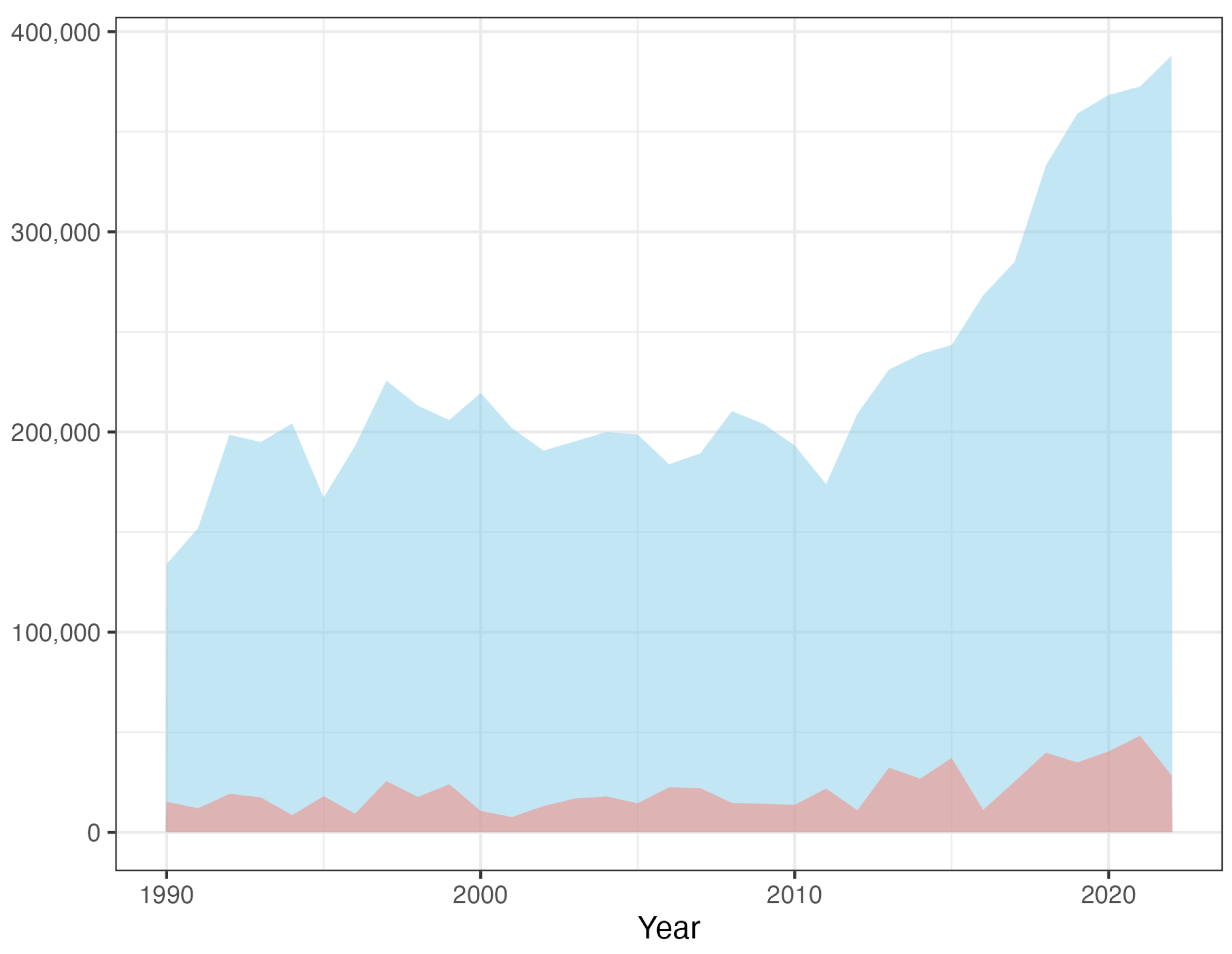
Figure 2.
Yearly normalized number of hailstorm claims and its linear trend.
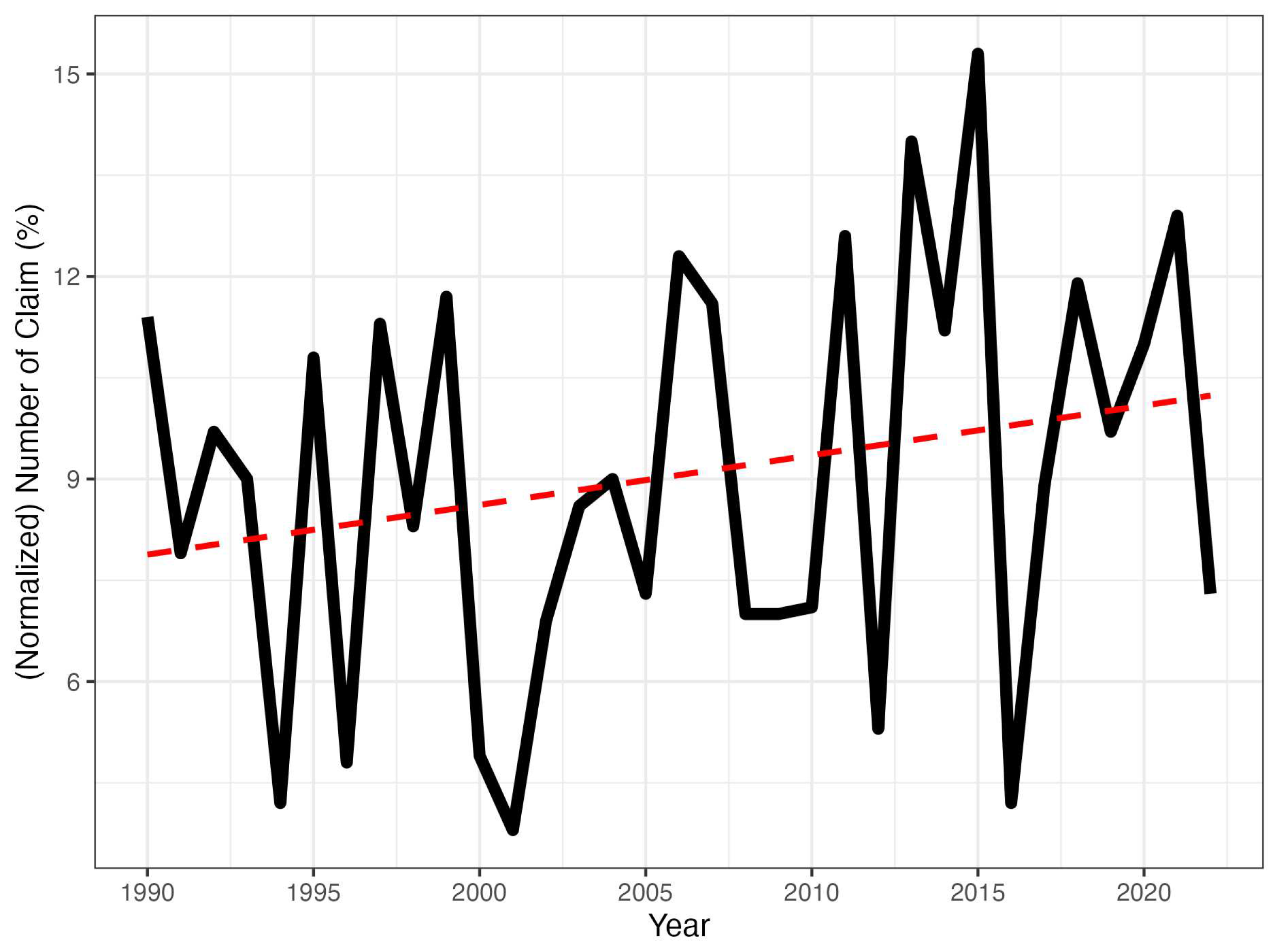
Figure 3.
Monthly number of claims (normalized) from January 1990 to December. 2022.
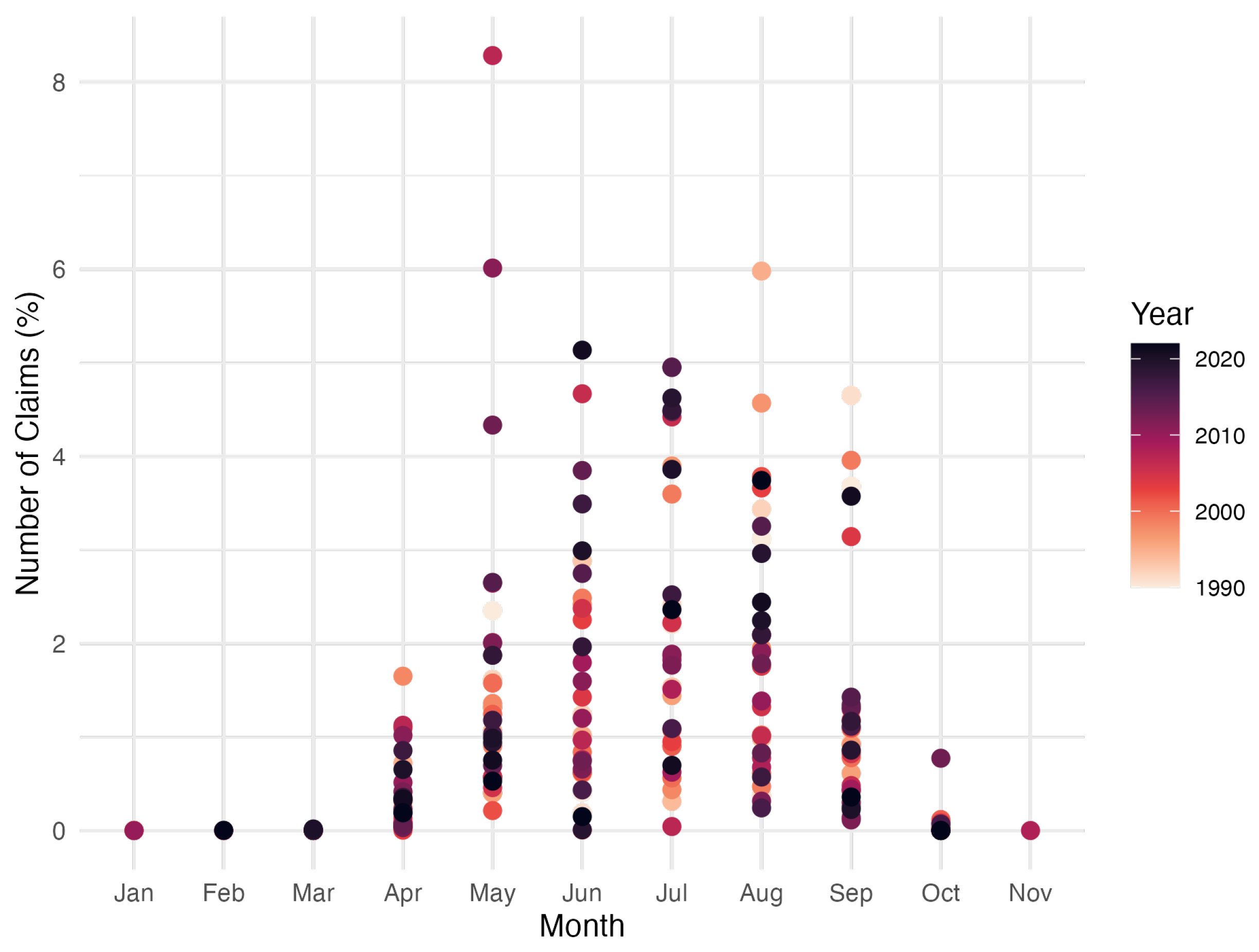
Figure 4.
Yearly Normalized .
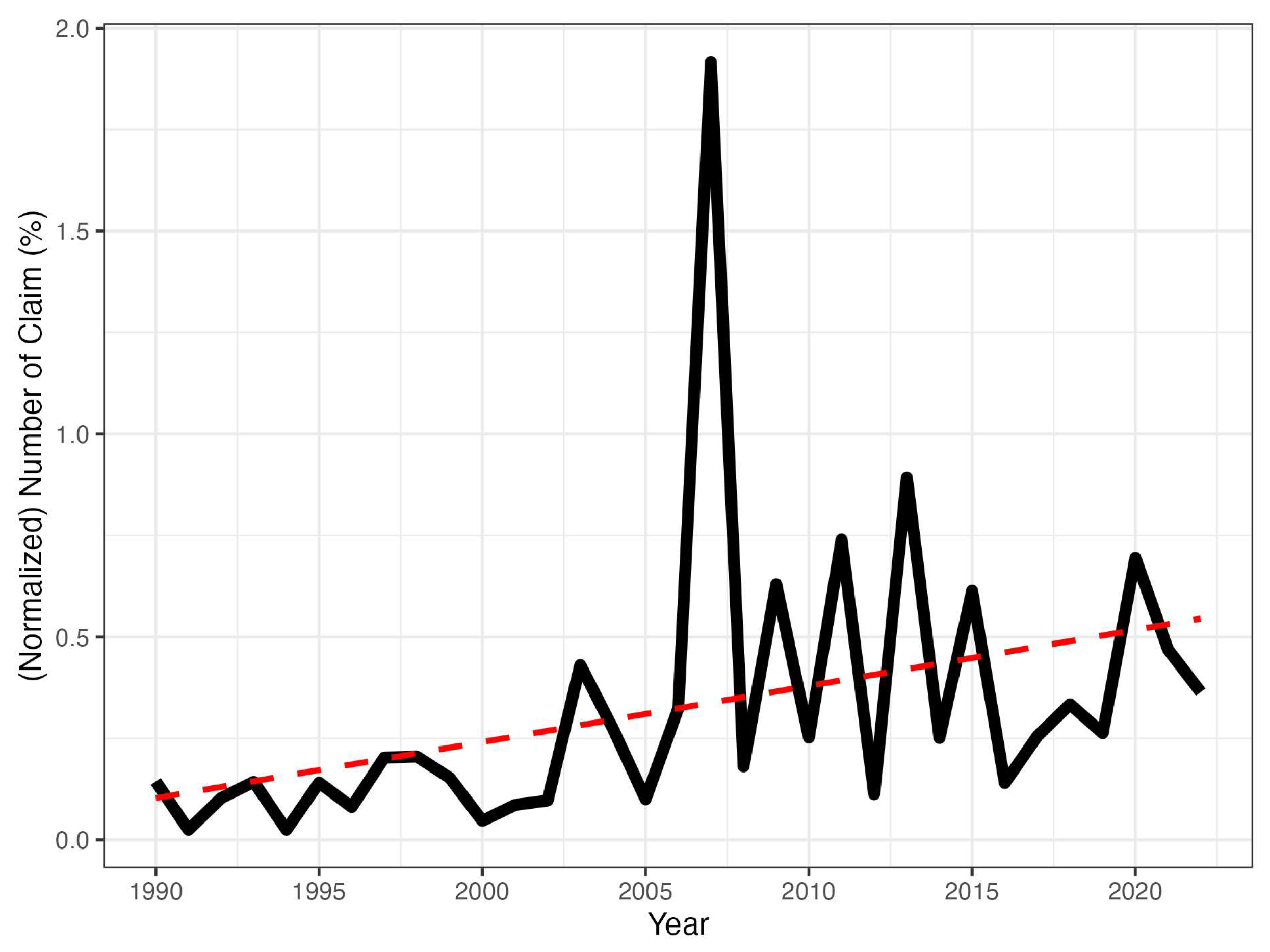
Figure 5.
Monthly total losses for the period January 1990-December 2022. The light blue points are the homogeneous losses, and the dark blue points are their logarithms.
Figure 5.
Monthly total losses for the period January 1990-December 2022. The light blue points are the homogeneous losses, and the dark blue points are their logarithms.
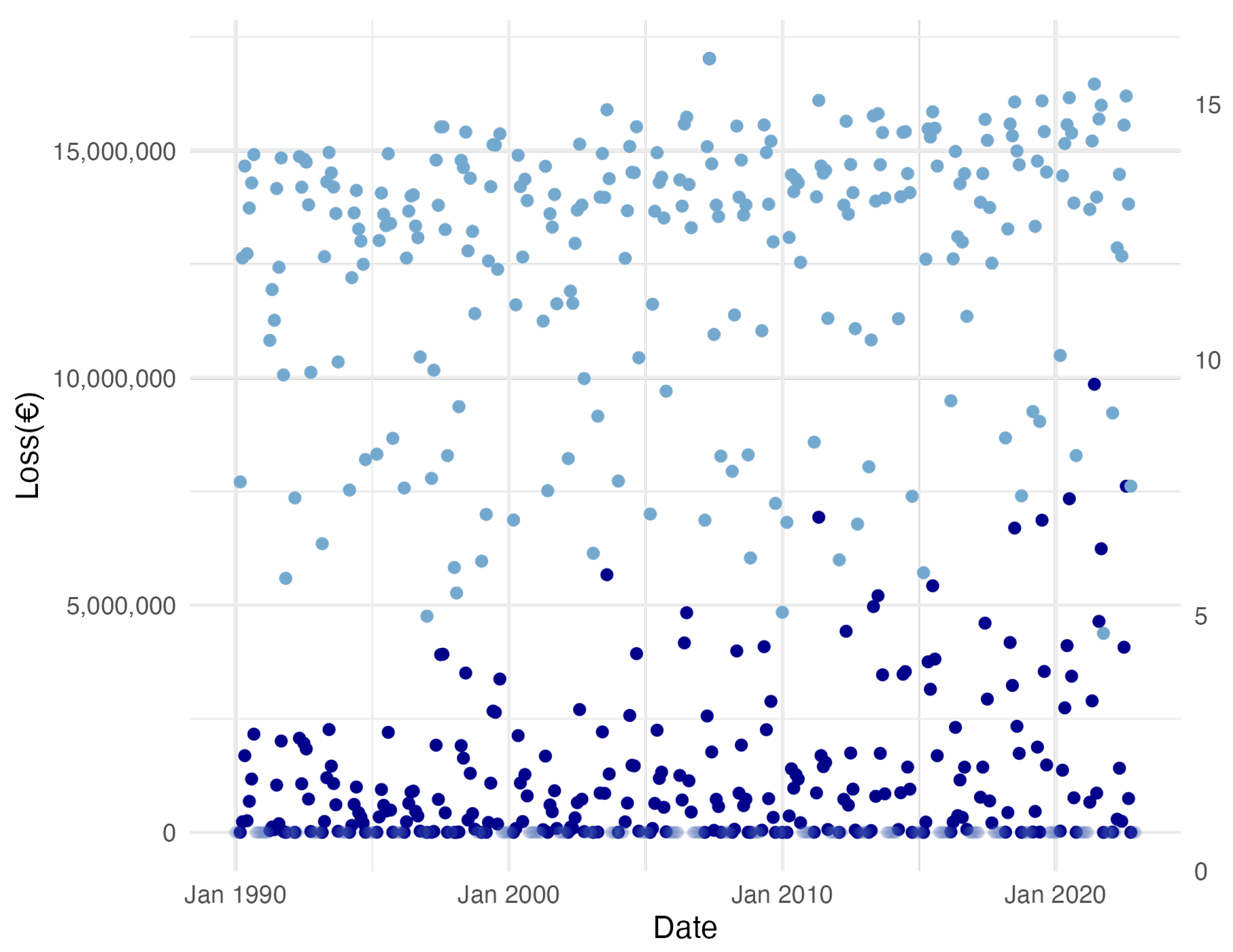
Figure 6.
Yearly total loss quantiles

Figure 7.
Annual SACI Variation from April to September (1961-2022) as an indicator of climate change during the hailstorm season.
Figure 7.
Annual SACI Variation from April to September (1961-2022) as an indicator of climate change during the hailstorm season.
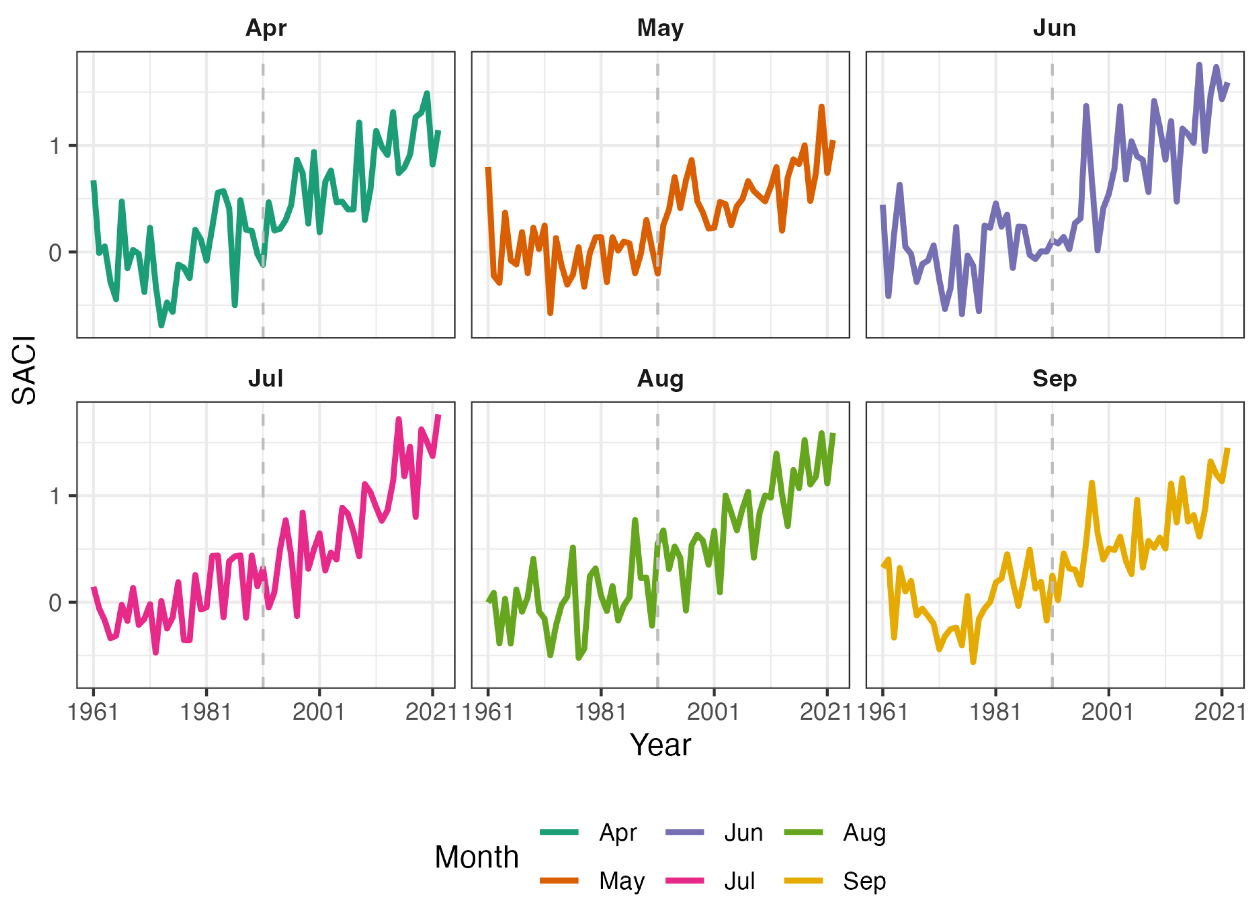
Figure 8.
Scatter plot of the monthly normalized number of claims N versus the SACI. Regression and quantile regression (probabilities ) lines corresponding to models 1 (eq.(7), Table 3) and model 4 (eq.(10), Table 4).
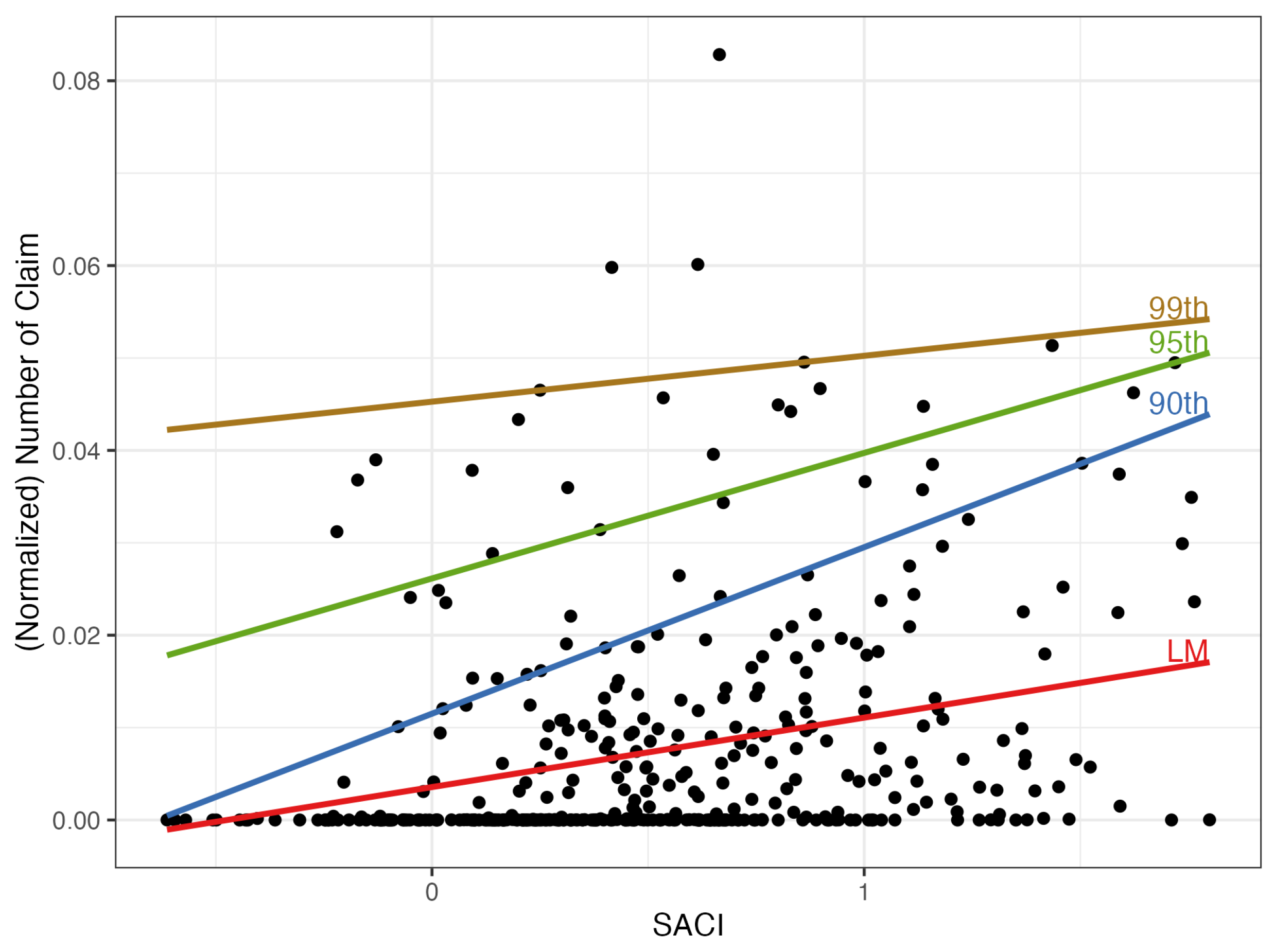
Figure 9.
Scatter plot of versus SACI. The lines represent linear regression and quantile regressions for three different quantiles (0.9, 0.95, and 0.99) corresponding to models 6 and 8.
Figure 9.
Scatter plot of versus SACI. The lines represent linear regression and quantile regressions for three different quantiles (0.9, 0.95, and 0.99) corresponding to models 6 and 8.
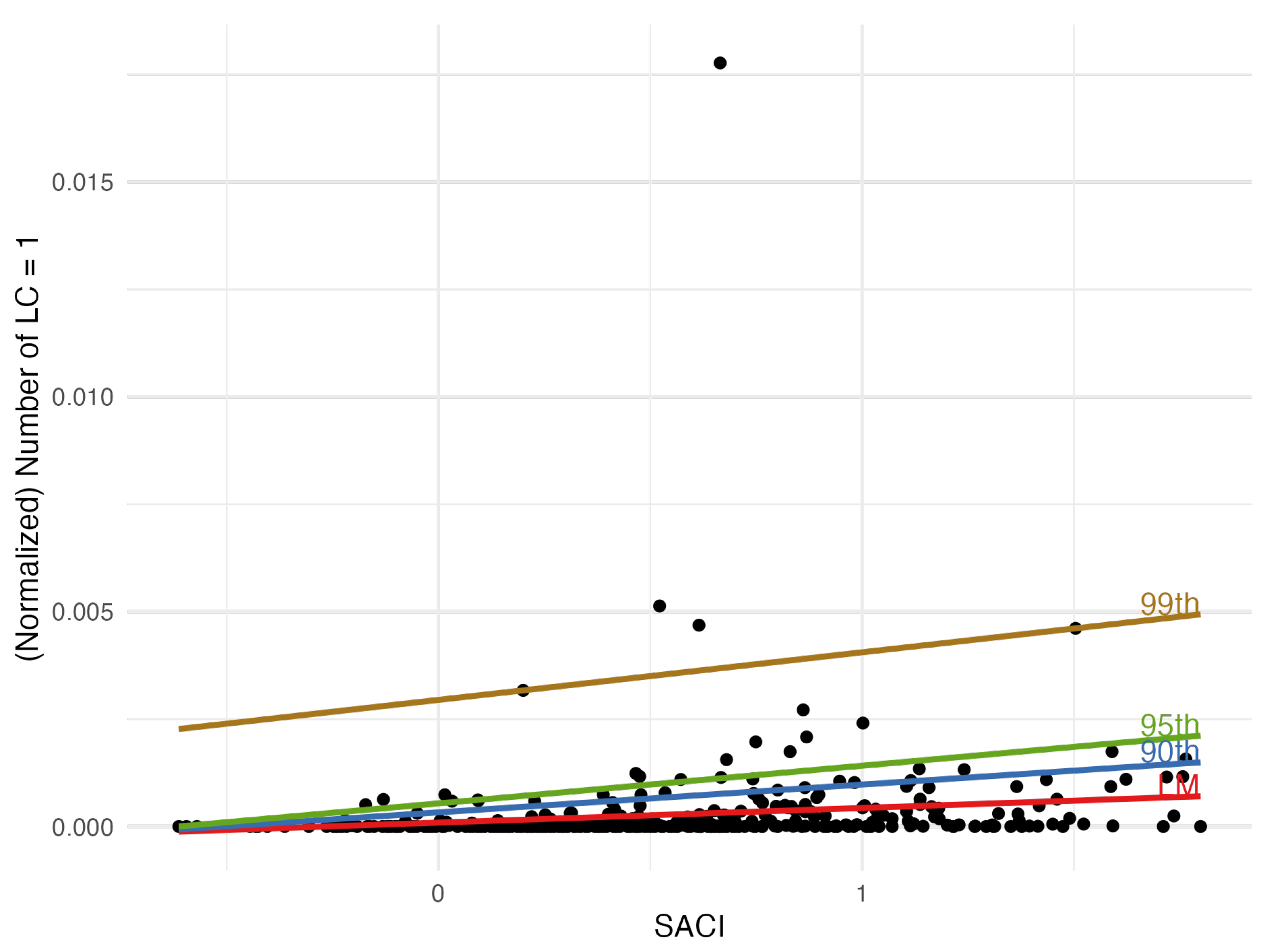
Figure 10.
Scatter plot of monthly versus SACI. Note: The straight lines are linear regression (see Table 9) and quantile regression ()(see Table 10).
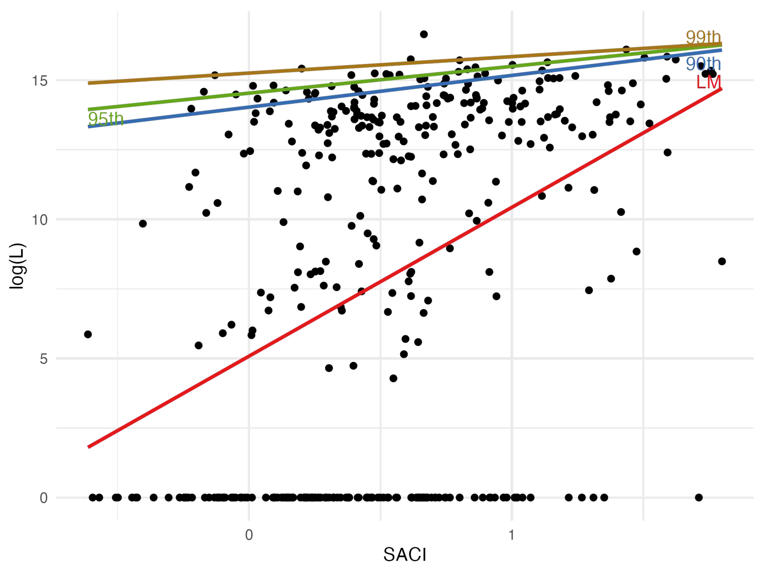

Table 1.
Spanish Wine Grape Insurance Data, yearly figures.
| Year | Total Insured sum (€) | Total Loss (€) | Crop Yield () | Number Of Policies | Number Of Plots | Number Of Claims |
|---|---|---|---|---|---|---|
| 1990 | 217,652,835 | 6,200,518 | 1,388,430,463 | 28,100 | 134,050 | 15,291 |
| 1991 | 248,557,853 | 3,560,276 | 1,550,473,335 | 31,621 | 152,005 | 12,000 |
| 1992 | 307,714,572 | 7,904,540 | 1,912,566,029 | 39,929 | 198,611 | 19,235 |
| 1993 | 284,919,972 | 6,826,730 | 1,829,365,370 | 37,832 | 195,007 | 17,456 |
| 1994 | 297,271,994 | 2,738,423 | 1,901,295,250 | 38,984 | 204,313 | 8,619 |
| 1995 | 242,077,610 | 5,569,047 | 1,400,284,025 | 29,129 | 167,305 | 18,063 |
| 1996 | 327,901,655 | 4,593,910 | 1,605,894,257 | 32,859 | 193,004 | 9,282 |
| 1997 | 395,633,563 | 14,096,834 | 1,957,379,446 | 37,049 | 225,642 | 25,611 |
| 1998 | 441,049,489 | 13,007,045 | 1,971,311,184 | 34,288 | 213,158 | 17,656 |
| 1999 | 437,265,055 | 14,794,992 | 1,917,674,498 | 32,706 | 206,014 | 24,029 |
| 2000 | 568,328,639 | 9,741,835 | 2,090,534,475 | 34,000 | 219,489 | 10,682 |
| 2001 | 560,603,175 | 6,759,693 | 2,011,166,692 | 30,996 | 201,894 | 7,641 |
| 2002 | 522,149,823 | 7,945,331 | 1,943,561,894 | 28,876 | 190,731 | 13,152 |
| 2003 | 562,951,706 | 18,847,196 | 2,076,438,149 | 29,037 | 195,308 | 16,855 |
| 2004 | 598,344,779 | 18,271,523 | 2,163,019,536 | 28,823 | 199,977 | 17,954 |
| 2005 | 595,592,273 | 10,960,930 | 2,098,146,664 | 26,412 | 198,760 | 14,503 |
| 2006 | 551,669,449 | 23,246,532 | 1,899,984,824 | 23,194 | 183,900 | 22,537 |
| 2007 | 577,020,427 | 42,553,289 | 1,964,259,110 | 22,665 | 189,357 | 22,043 |
| 2008 | 653,256,796 | 15,265,573 | 2,230,822,485 | 24,461 | 210,449 | 14,725 |
| 2009 | 628,159,377 | 19,773,933 | 2,097,168,866 | 21,950 | 204,072 | 14,280 |
| 2010 | 597,317,970 | 10,530,360 | 1,951,036,257 | 19,993 | 193,284 | 13,732 |
| 2011 | 516,300,441 | 23,659,028 | 1,746,476,820 | 17,927 | 174,013 | 21,883 |
| 2012 | 644,892,414 | 15,259,638 | 2,292,548,909 | 21,480 | 209,162 | 11,043 |
| 2013 | 630,157,964 | 30,235,918 | 2,268,987,633 | 21,075 | 231,153 | 32,294 |
| 2014 | 687,759,537 | 18,986,141 | 2,389,698,870 | 20,650 | 238,865 | 26,823 |
| 2015 | 704,818,295 | 33,449,574 | 2,426,866,357 | 20,139 | 243,458 | 37,138 |
| 2016 | 772,792,789 | 11,049,778 | 2,633,586,202 | 20,947 | 268,232 | 11,205 |
| 2017 | 821,585,396 | 20,152,939 | 2,768,418,806 | 21,023 | 284,922 | 25,283 |
| 2018 | 939,523,058 | 37,068,415 | 3,010,843,844 | 22,839 | 333,156 | 39,809 |
| 2019 | 1,028,808,795 | 29,643,282 | 3,154,082,113 | 23,467 | 359,053 | 34,916 |
| 2020 | 1,038,651,982 | 41,498,451 | 3,159,232,107 | 23,636 | 368,346 | 40,465 |
| 2021 | 1,056,633,225 | 53,137,810 | 3,192,077,192 | 23,537 | 372,611 | 48,217 |
| 2022 | 1,091,289,076 | 30,551,509 | 3,279,107,478 | 23,520 | 387,991 | 28,479 |
Table 2.
The normalized monthly number of claims.
| Jan | Feb | Mar | Apr | May | Jun | Jul | Aug | Sep | Oct | Nov | Dec | |
|---|---|---|---|---|---|---|---|---|---|---|---|---|
| 1990 | 0.0015 | 0.3081 | 2.3514 | 0.4118 | 1.5308 | 3.1197 | 3.6792 | |||||
| 1991 | 0.0408 | 0.4092 | 0.1895 | 2.2058 | 0.3756 | 4.6512 | 0.0164 | 0.0007 | ||||
| 1992 | 0.0030 | 1.6162 | 1.2416 | 2.4082 | 3.4349 | 0.9415 | 0.0227 | |||||
| 1993 | 0.0021 | 0.3123 | 1.3200 | 2.8835 | 1.5353 | 1.9061 | 0.9230 | 0.0692 | ||||
| 1994 | 0.0015 | 0.4033 | 1.0053 | 1.2045 | 0.3132 | 0.9862 | 0.2966 | 0.0078 | ||||
| 1995 | 0.0048 | 0.7208 | 1.0663 | 1.0185 | 0.9091 | 5.9801 | 1.0831 | 0.0030 | ||||
| 1996 | 0.0047 | 0.3280 | 0.4000 | 0.9746 | 1.4430 | 1.0098 | 0.6124 | 0.0326 | ||||
| 1997 | 0.0004 | 0.0049 | 0.0315 | 1.3145 | 0.6107 | 3.8978 | 4.5687 | 0.9161 | 0.0031 | |||
| 1998 | 0.0033 | 0.0009 | 0.0033 | 1.6504 | 1.3586 | 2.4189 | 0.4372 | 1.9502 | 0.4199 | 0.0403 | ||
| 1999 | 0.0005 | 0.0010 | 0.2451 | 0.9053 | 2.4848 | 3.5968 | 0.4713 | 3.9575 | ||||
| 2000 | 0.0023 | 0.0838 | 1.5768 | 0.8388 | 0.5627 | 1.0215 | 0.7795 | |||||
| 2001 | 0.0490 | 1.2437 | 0.0064 | 0.9000 | 0.6142 | 0.8524 | 0.1184 | |||||
| 2002 | 0.0005 | 0.0661 | 0.2144 | 0.6218 | 1.0785 | 3.7844 | 1.0963 | 0.0131 | ||||
| 2003 | 0.0005 | 0.0046 | 0.5765 | 2.2529 | 0.9503 | 3.6619 | 1.1833 | |||||
| 2004 | 0.0020 | 0.1340 | 0.5636 | 1.4272 | 1.8632 | 1.7572 | 3.1424 | 0.0835 | ||||
| 2005 | 0.0010 | 0.0795 | 0.4593 | 2.3747 | 2.2228 | 1.3232 | 0.8226 | 0.0136 | ||||
| 2006 | 1.0962 | 0.5753 | 4.6688 | 4.4209 | 1.0120 | 0.4818 | ||||||
| 2007 | 0.0037 | 1.1259 | 8.2833 | 0.9670 | 0.0438 | 0.7763 | 0.4309 | 0.0048 | ||||
| 2008 | 0.0048 | 0.0889 | 2.6448 | 0.7579 | 1.5101 | 0.6781 | 1.2972 | 0.0048 | 0.0010 | |||
| 2009 | 0.0304 | 2.0101 | 1.7969 | 0.6243 | 2.0924 | 0.4425 | 0.0010 | |||||
| 2010 | 0.0005 | 0.0021 | 0.5143 | 1.8755 | 1.2003 | 1.8227 | 1.3855 | 0.3032 | ||||
| 2011 | 0.0086 | 1.0183 | 6.0122 | 1.5964 | 1.8861 | 1.9119 | 0.1419 | |||||
| 2012 | 0.0010 | 0.4174 | 2.0032 | 0.6574 | 1.7685 | 0.3151 | 0.1143 | 0.0029 | ||||
| 2013 | 0.0017 | 0.0346 | 4.3339 | 0.7419 | 4.9547 | 1.7841 | 1.3454 | 0.7735 | ||||
| 2014 | 0.0599 | 0.6962 | 3.8486 | 4.4770 | 0.8302 | 1.3162 | 0.0013 | |||||
| 2015 | 0.0008 | 0.2234 | 2.6530 | 2.7483 | 4.9491 | 3.2531 | 1.4265 | |||||
| 2016 | 0.0112 | 0.1831 | 1.0293 | 0.4351 | 1.0908 | 0.2427 | 1.1151 | 0.0701 | ||||
| 2017 | 0.8560 | 1.1796 | 3.4915 | 2.5200 | 0.5728 | 0.2538 | ||||||
| 2018 | 0.0018 | 0.3554 | 1.8739 | 1.9648 | 4.4922 | 2.0924 | 1.1679 | 0.0006 | ||||
| 2019 | 0.0042 | 0.3228 | 0.9428 | 0.0089 | 4.6236 | 2.9622 | 0.8600 | |||||
| 2020 | 0.0176 | 0.6532 | 0.9893 | 2.9904 | 3.8605 | 2.2446 | 0.2259 | 0.0041 | ||||
| 2021 | 0.3387 | 0.7536 | 5.1348 | 0.6975 | 2.4414 | 3.5740 | 0.0003 | |||||
| 2022 | 0.0034 | 0.1925 | 0.5289 | 0.1497 | 2.3617 | 3.7429 | 0.3593 | 0.0018 |
Table 3.
Linear Regression Results for N, Models 1, 2, and 3, (see equations (7), (8), and (9)). For each independent variable, we show the value, the p-value( *, **, ***), and the standard deviation in parenthesis.
| Dependent variable: | |||
| Number of Claim | |||
| Model 1 | Model 2 | Model 3 | |
| SACI | 0.008*** | ||
| (0.001) | |||
| T90std | 0.002*** | 0.001 | |
| (0.001) | (0.001) | ||
| T10std | 0.002 | 0.0005 | |
| (0.001) | (0.001) | ||
| Pstd | -0.002 | 0.003*** | |
| (0.001) | (0.001) | ||
| Dstd | -0.001 | -0.0001 | |
| (0.001) | (0.001) | ||
| Wstd | -0.001 | -0.003*** | |
| (0.001) | (0.001) | ||
| Sstd | 0.002*** | 0.0004 | |
| (0.0004) | (0.0004) | ||
| April | 0.003* | ||
| (0.002) | |||
| May | 0.017*** | ||
| (0.002) | |||
| June | 0.017*** | ||
| (0.002) | |||
| July | 0.023*** | ||
| (0.002) | |||
| August | 0.020*** | ||
| (0.002) | |||
| September | 0.013*** | ||
| (0.002) | |||
| Constant | 0.004*** | 0.003*** | -0.0002 |
| (0.001) | (0.001) | (0.001) | |
| Observations | 396 | 396 | 396 |
| R2 | 0.081 | 0.138 | 0.502 |
| Adjusted R2 | 0.079 | 0.125 | 0.487 |
| Residual Std. Error | 0.012 (df = 394) | 0.012 (df = 389) | 0.009 (df = 383) |
| F Statistic | 34.868*** (df = 1; 394) | 10.398*** (df = 6; 389) | 32.197*** (df = 12; 383) |
Note:*
Table 4.
Quantile Regression Results for model 4 (eq. 10)
Table 4.
Quantile Regression Results for model 4 (eq. 10)
| Dependent variable: | |||
| Number of Claim ( Normalized) | |||
| = 0.9 | = 0.95 | = 0.99 | |
| SACI | 0.018*** | 0.014 | 0.005* |
| (0.013,0.023) | (-0.004,0.031) | (-0.001,0.011) | |
| Constant | 0.012*** | 0.026*** | 0.045*** |
| (0.008,0.015) | (0.014,0.038) | (0.041,0.049) | |
| Observations | 396 | 396 | 396 |
| Pseudo | 0.0928 | 0.0420 | 0.0173 |
Note: *
Table 5.
Results for quantile regression for the normalized number of claims, N.
| Dependent variable: | ||||||
| Number of Claim ( Normalized) | ||||||
| Model 50.9 | Model 50.95 | Model 50.99 | Model 60.9 | Model 60.95 | Model 60.99 | |
| SACI | 0.0001*** | 0.0001*** | 0.0008*** | |||
| (0.00003,0.0001) | (0.0001,0.0002) | (0.0007,0.0010) | ||||
| T90std | 0.00003*** | 0.0002*** | 0.0017*** | |||
| (0.00002,0.00005) | (0.0001,0.0002) | (0.0015,0.0019) | ||||
| T10std | 0.0001*** | 0.0001** | 0.0009*** | |||
| (0.00003,0.0001) | (0.000003,0.0002) | (0.0006,0.0013) | ||||
| Pstd | 0.0001*** | 0.0003*** | 0.0019*** | |||
| (0.00005,0.0001) | (0.0002,0.0004) | (0.0015,0.0022) | ||||
| Dstd | -0.00002 | 0.0001 | 0.0003 | |||
| (-0.0001,0.00001) | (-0.00002,0.0002) | (-0.0001,0.0007) | ||||
| Wstd | -0.00005*** | -0.0001*** | -0.0017*** | |||
| (-0.0001,-0.00003) | (-0.0002,-0.0001) | (-0.0020,-0.0015) | ||||
| Sstd | 0.00002*** | 0.0001*** | 0.0008*** | |||
| (0.00002,0.00003) | (0.00002,0.0001) | (0.0007,0.0010) | ||||
| April | 0.0101*** | 0.0111*** | 0.0153*** | 0.0099*** | 0.0105*** | 0.0163*** |
| (0.0100,0.0101) | (0.0110,0.0112) | (0.0150,0.0156) | (0.0099,0.0100) | (0.0104,0.0107) | (0.0157,0.0169) | |
| May | 0.0264*** | 0.0600*** | 0.0817*** | 0.0265*** | 0.0596*** | 0.0798*** |
| (0.0264,0.0265) | (0.0599,0.0601) | (0.0814,0.0819) | (0.0264,0.0265) | (0.0594,0.0598) | (0.0792,0.0804) | |
| June | 0.0348*** | 0.0465*** | 0.0495*** | 0.0347*** | 0.0461*** | 0.0422*** |
| (0.0347,0.0348) | (0.0464,0.0466) | (0.0493,0.0498) | (0.0346,0.0347) | (0.0459,0.0463) | (0.0415,0.0428) | |
| July | 0.0448*** | 0.0492*** | 0.0482*** | 0.0448*** | 0.0483*** | 0.0432*** |
| (0.0448,0.0449) | (0.0491,0.0493) | (0.0480,0.0485) | (0.0447,0.0448) | (0.0481,0.0484) | (0.0426,0.0439) | |
| August | 0.0373*** | 0.0455*** | 0.0589*** | 0.0372*** | 0.0449*** | 0.0572*** |
| (0.0373,0.0374) | (0.0454,0.0456) | (0.0586,0.0591) | (0.0371,0.0372) | (0.0448,0.0451) | (0.0566,0.0579) | |
| September | 0.0356*** | 0.0394*** | 0.0457*** | 0.0355*** | 0.0392*** | 0.0423*** |
| (0.0356,0.0357) | (0.0393,0.0395) | (0.0454,0.0460) | (0.0355,0.0356) | (0.0390,0.0394) | (0.0416,0.0429) | |
| Constant | 0.00003*** | 0.0001*** | 0.0006*** | 0.0001*** | 0.0003*** | 0.0020*** |
| (0.00001,0.0001) | (0.00004,0.0001) | (0.0005,0.0007) | (0.0001,0.0001) | (0.0002,0.0004) | (0.0017,0.0023) | |
| Observations | 396 | 396 | 396 | 396 | 396 | 396 |
| Pseudo | 0.5607 | 0.5771 | 0.5780 | 0.5609 | 0.5780 | 0.6475 |
Note: *p<0.1; **p <0.05; ***p<0.01
Table 6.
Linear Regression for Number of Loss Cost = 1
| Dependent variable: | ||
| Number of Cliam (Loss Cost = 1) | ||
| Model 7 | Model 8 | |
| SACI | 0.0003*** | 0.0002* |
| (0.0001) | (0.0001) | |
| April | -0.00001 | |
| (0.0002) | ||
| May | 0.001*** | |
| (0.0002) | ||
| June | 0.0003 | |
| (0.0002) | ||
| July | 0.001*** | |
| (0.0002) | ||
| August | 0.0004** | |
| (0.0002) | ||
| September | 0.0002 | |
| (0.0002) | ||
| Constant | 0.0001 | -0.0001 |
| (0.0001) | (0.0001) | |
| Observations | 396 | 396 |
| R2 | 0.024 | 0.146 |
| Adjusted R2 | 0.021 | 0.131 |
| Residual Std. Error | 0.001 (df = 394) | 0.001 (df = 388) |
| F Statistic | 9.608*** (df = 1; 394) | 9.475*** (df = 7; 388) |
Note: *p<0.1; **p<0.05; ***p<0.01
Table 7.
Quantile Regression Results for model 9 (eq. 15).
Table 7.
Quantile Regression Results for model 9 (eq. 15).
| Dependent variable: | |||
| 90th | 95th | 99th | |
| SACI | 0.001*** | 0.001*** | 0.001 |
| (0.0004,0.001) | (0.001,0.001) | (-0.008,0.010) | |
| Constant | 0.0003*** | 0.001*** | 0.003 |
| (0.0001,0.001) | (0.0003,0.001) | (-0.003,0.009) | |
| Observations | 396 | 396 | 396 |
| Pseudo | 0.0967 | 0.0742 | 0.0411 |
Note:*p<0.1; **p<0.05; ***p<0.01
Table 8.
Quantile Regression Results for
| Dependent variable: | ||||||
| Number of ( Normalized) | ||||||
| Mod 10 | Mod 10 | Mod 10 | Mod 11 | Mod 11 | Mod 11 | |
| SACI | 0.000 | 0.00000*** | 0.0003*** | |||
| (-0.0003,0.0003) | (0.00000,0.00001) | (0.0002,0.0003) | ||||
| T90std | 0.004*** | 0.010*** | 0.016*** | |||
| (0.003,0.004) | (0.009,0.011) | (0.016,0.017) | ||||
| T10std | 0.001** | 0.004*** | 0.003*** | |||
| (0.0001,0.002) | (0.002,0.006) | (0.001,0.004) | ||||
| Pstd | 0.0001 | 0.0001 | 0.0001 | |||
| (-0.001,0.001) | (-0.002,0.002) | (-0.001,0.001) | ||||
| Dstd | -0.0004 | 0.0002 | -0.001 | |||
| (-0.002,0.001) | (-0.002,0.002) | (-0.002,0.001) | ||||
| Wstd | -0.002*** | -0.003*** | -0.001 | |||
| (-0.003,-0.001) | (-0.004,-0.001) | (-0.002,0.0002) | ||||
| Sstd | 0.001*** | 0.002*** | -0.0001 | |||
| (0.001,0.001) | (0.001,0.003) | (-0.001,0.0003) | ||||
| April | 0.0002 | 0.0002*** | 0.0001 | 0.013*** | 0.008*** | 0.005*** |
| (-0.0002,0.001) | (0.0002,0.0002) | (-0.0001,0.0002) | (0.011,0.015) | (0.005,0.011) | (0.003,0.007) | |
| May | 0.003*** | 0.005*** | 0.017*** | 0.314*** | 0.493*** | 1.760*** |
| (0.003,0.004) | (0.005,0.005) | (0.017,0.018) | (0.313,0.316) | (0.490,0.497) | (1.758,1.762) | |
| June | 0.001*** | 0.001*** | 0.001*** | 0.096*** | 0.102*** | 0.106*** |
| (0.001,0.002) | (0.001,0.001) | (0.001,0.001) | (0.094,0.098) | (0.098,0.105) | (0.104,0.109) | |
| July | 0.002*** | 0.003*** | 0.004*** | 0.134*** | 0.248*** | 0.403*** |
| (0.001,0.002) | (0.003,0.003) | (0.004,0.004) | (0.131,0.136) | (0.245,0.251) | (0.401,0.405) | |
| August | 0.001*** | 0.002*** | 0.002*** | 0.095*** | 0.123*** | 0.168*** |
| (0.001,0.002) | (0.002,0.002) | (0.002,0.002) | (0.092,0.097) | (0.119,0.126) | (0.166,0.170) | |
| September | 0.001*** | 0.001*** | 0.002*** | 0.061*** | 0.122*** | 0.183*** |
| (0.0002,0.001) | (0.001,0.001) | (0.002,0.002) | (0.059,0.063) | (0.119,0.126) | (0.181,0.186) | |
| Constant | 0.000 | 0.00000** | 0.0002*** | 0.002*** | 0.005*** | 0.012*** |
| (-0.0002,0.0002) | (0.00000,0.00000) | (0.0001,0.0002) | (0.001,0.003) | (0.004,0.007) | (0.011,0.013) | |
| Observations | 396 | 396 | 396 | 396 | 396 | 396 |
| Pseudo | 0.3559 | 0.4101 | 0.7156 | 0.3585 | 0.4150 | 0.7275 |
Note: *p<0.1; **p<0.05; ***p<0.01
Table 9.
Results of linear regression models for .
| Dependent variable: | ||||
| model 12 | model 13 | model 14 | model 15 | |
| SACI | 5.350∗∗∗ | 0.878∗∗∗ | ||
| (0.620) | (0.327) | |||
| T90std | 0.737∗∗∗ | 0.226 | ||
| (0.331) | (0.180) | |||
| T10std | 1.204∗ | 0.621∗ | ||
| (0.640) | (0.328) | |||
| Pstd | −2.350∗∗∗ | 0.023 | ||
| (0.532) | (0.289) | |||
| Dstd | −0.312 | 0.414 | ||
| (0.692) | (0.352) | |||
| Wstd | 0.723 | −0.388∗ | ||
| (0.442) | (0.229) | |||
| Sstd | 1.759∗∗∗ | 0.344∗∗∗ | ||
| (0.195) | (0.112) | |||
| April | 9.371∗∗∗ | 9.214∗∗∗ | ||
| (0.541) | (0.542) | |||
| May | 11.861∗∗∗ | 11.863∗∗∗ | ||
| (0.533) | (0.533) | |||
| June | 11.066∗∗∗ | 10.852∗∗∗ | ||
| (0.553) | (0.595) | |||
| July | 11.547∗∗∗ | 11.360∗∗∗ | ||
| (0.547) | (0.580) | |||
| August | 11.482∗∗∗ | 11.385∗∗∗ | ||
| (0.549) | (0.562) | |||
| September | 11.028∗∗∗ | 10.853∗∗∗ | ||
| (0.538) | (0.575) | |||
| Constant | 5.083∗∗∗ | 1.922∗∗∗ | 4.444∗∗∗ | 1.925∗∗∗ |
| (0.441) | (0.230) | (0.454) | (0.243) | |
| Observations | 396 | 396 | 396 | 396 |
| R2 | 0.159 | 0.809 | 0.266 | 0.814 |
| Adjusted R2 | 0.157 | 0.805 | 0.255 | 0.808 |
| Residual Std. Error | 5.859 (df = 394) | 2.815 (df = 388) | 5.509 (df = 389) | 2.794 (df = 383) |
| F Statistic | 74.511∗∗∗ (df = 1; 394) | 234.536∗∗∗ (df = 7; 388) | 23.497∗∗∗ (df = 6; 389) | 139.809∗∗∗ (df = 12; 383) |
Table 10.
Results of quantile regression for model 16 (eq. 24)
Table 10.
Results of quantile regression for model 16 (eq. 24)
| Dependent variable: | |||
| 90th | 95th | 99th | |
| SACI | 1.141*** | 0.963*** | 0.591 |
| (0.480,1.802) | (0.467,1.458) | (-0.274,1.455) | |
| Constant | 14.031*** | 14.536*** | 15.256*** |
| (13.561,14.501) | (14.183,14.888) | (14.641,15.871) | |
| Observations | 396 | 396 | 396 |
| Pseudo | 0.0319 | 0.0304 | 0.0292 |
Note: *p<0.1; **p <0.05; ***p<0.01
Table 11.
Results of quantile regression for
| Dependent variable: | ||||||
| Model | Model | Model | Model | Model | Model | |
| SACI | 0.541* | 0.578** | 0.619*** | |||
| (-0.059,1.141) | (0.002,1.153) | (0.257,0.981) | ||||
| T90std | 0.085 | 0.218** | 0.332*** | |||
| (-0.128,0.299) | (0.032,0.404) | (0.183,0.481) | ||||
| T10std | 0.121 | 0.422** | 0.143 | |||
| (-0.268,0.510) | (0.083,0.760) | (-0.128,0.415) | ||||
| Pstd | 0.277 | 0.528*** | 1.101*** | |||
| (-0.065,0.619) | (0.231,0.826) | (0.863,1.340) | ||||
| Dstd | 0.169 | 0.066 | 0.876*** | |||
| (-0.248,0.587) | (-0.297,0.429) | (0.585,1.167) | ||||
| Wstd | -0.338** | -0.268** | -0.484*** | |||
| (-0.609,-0.067) | (-0.504,-0.032) | (-0.673,-0.295) | ||||
| Sstd | 0.168** | 0.148** | 0.020 | |||
| (0.036,0.300) | (0.033,0.264) | (-0.073,0.112) | ||||
| April | 5.331*** | 4.495*** | 3.203*** | 5.165*** | 4.703*** | 3.826*** |
| (4.338,6.324) | (3.543,5.447) | (2.604,3.802) | (4.522,5.808) | (4.144,5.263) | (3.378,4.275) | |
| May | 6.994*** | 5.857*** | 4.934*** | 7.084*** | 6.077*** | 5.233*** |
| (6.015,7.974) | (4.917,6.796) | (4.343,5.525) | (6.453,7.716) | (5.528,6.627) | (4.792,5.673) | |
| June | 6.717*** | 5.249*** | 3.911*** | 6.594*** | 5.672*** | 4.694*** |
| (5.702,7.732) | (4.275,6.222) | (3.299,4.523) | (5.889,7.299) | (5.059,6.285) | (4.202,5.185) | |
| July | 7.003*** | 5.715*** | 3.955*** | 6.657*** | 5.707*** | 4.560*** |
| (5.998,8.008) | (4.750,6.679) | (3.348,4.561) | (5.970,7.344) | (5.109,6.305) | (4.081,5.039) | |
| August | 6.767*** | 5.388*** | 3.625*** | 6.387*** | 5.317*** | 3.719*** |
| (5.759,7.776) | (4.420,6.355) | (3.017,4.234) | (5.720,7.054) | (4.737,5.897) | (3.253,4.184) | |
| September | 6.687*** | 5.420*** | 3.639*** | 6.622*** | 5.624*** | 4.528*** |
| (5.700,7.675) | (4.473,6.367) | (3.043,4.235) | (5.940,7.303) | (5.032,6.217) | (4.052,5.003) | |
| Constant | 7.992*** | 9.540*** | 11.305*** | 8.142*** | 9.439*** | 11.018*** |
| (7.570,8.414) | (9.135,9.945) | (11.050,11.560) | (7.854,8.430) | (9.189,9.690) | (10.817,11.219) | |
| Observations | 396 | 396 | 396 | 396 | 396 | 396 |
| Pseudo | 0.3711 | 0.3192 | 0.2531 | 0.38 | 0.3354 | 0.2857 |
Note: *p<0.1; **p <0.05; ***p<0.01
Disclaimer/Publisher’s Note: The statements, opinions and data contained in all publications are solely those of the individual author(s) and contributor(s) and not of MDPI and/or the editor(s). MDPI and/or the editor(s) disclaim responsibility for any injury to people or property resulting from any ideas, methods, instructions or products referred to in the content. |
© 2024 by the authors. Licensee MDPI, Basel, Switzerland. This article is an open access article distributed under the terms and conditions of the Creative Commons Attribution (CC BY) license (http://creativecommons.org/licenses/by/4.0/).
Copyright: This open access article is published under a Creative Commons CC BY 4.0 license, which permit the free download, distribution, and reuse, provided that the author and preprint are cited in any reuse.


