Submitted:
28 December 2023
Posted:
30 December 2023
You are already at the latest version
Abstract
Active flow control is a promising technology for reducing noise, emissions, and power consumption in various applications. To better understand the performance of synthetic jet actuators, a computational model that couples structural mechanics with electrostatics, pressure acoustics, and fluid dynamics has been needed. The model presented here has been validated against experimental data and then used to investigate the fluid behavior inside and outside the synthetic jet actuator cavity, impacts of thermoviscous losses on capturing the acoustic response of the actuator, and viability of different modeling methods of diaphragms in computational simulations. The results capture the feedback from the fluid onto the diaphragm and highlight the need for careful acoustic modeling.
Keywords:
Synthetic Jets
; Flow Control
; Multiphysics Modeling
1. Introduction
Global efforts to reduce noise, emissions, and power consumption have led to rapid developments in the realm of active flow control - the addition of energy to a flow to change its aerodynamic characteristics. Passive flow control efforts, such as flaps on airplanes or slots on wind turbine blades [1] have been effective at improving efficiency, but active methods are required to achieve significant further improvements [2]. This will only become more important as technology such as aviation and wind power generation continue to grow in importance and popularity.
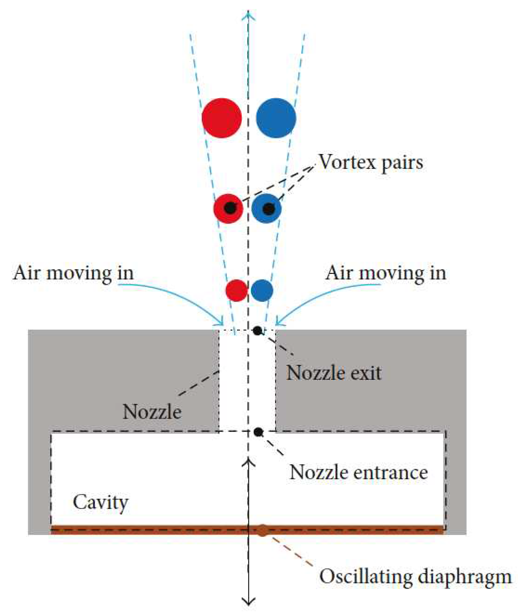
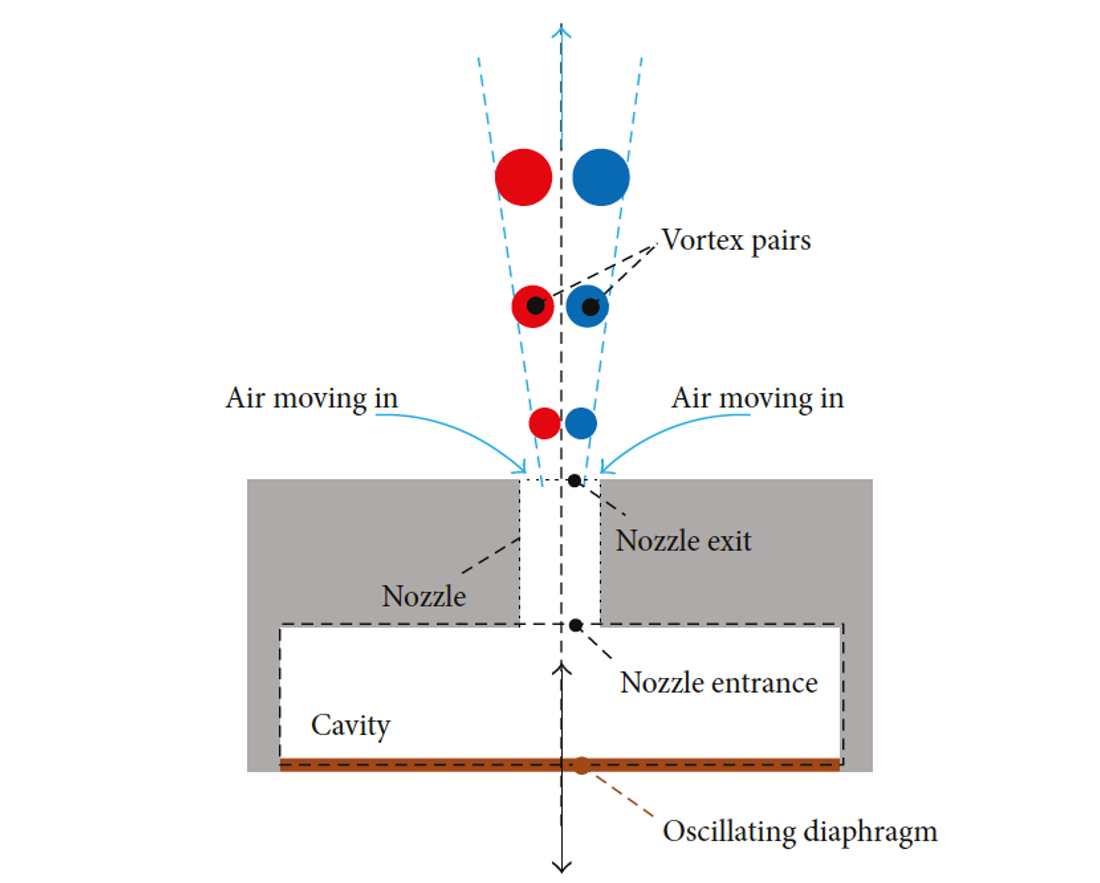
Figure 1.
Cross-section schematic of an opposite-facing piezoelectric synthetic jet actuator [3].
Synthetic jet actuators (SJAs) are simple active flow control devices with sizes generally on the order of millimeters. They are typically comprised of a cavity with one or more diaphragms mounted inside, and an orifice or nozzle which leads to the surface where energy addition is desired. By applying a time-varying sinusoidal electric potential, the piezoelectric disk - clamped around its edges - flexes inward and outward, effectively shrinking and enlarging the cavity of the SJA. The movement of the diaphragm creates an alternate ingestion and expulsion of fluid from the cavity.
These devices are advantageous because they can be implemented flush to a surface, introducing no parasitic drag. They are also compact, inexpensive, simple and require no external fluid supply. Their performance can also be manipulated by altering the voltage signal, meaning they can be tailored to different applications without requiring significant redesign. All of these advantages make synthetic jet actuators appealing devices for a wide range of fields.
A downside that SJAs present is their noise generation. Due to the vibration of the diaphragm, and resonance of the cavity, some designs generate significant noise [4–6]. Excessive noise generation can be a critical design drawback, especially in applications such as transportation, where noise reduction is a focus. Arafa et al. [7] found that when designing SJA arrays, an excitation frequency away from the cavity acoustic modes should be used to ensure uniform mean jet velocity across the array. They achieved this target by dividing the SJA cavity into isolated sections. Arafa et al. [8] revealed that it is possible to reduce the SJA noise by 8-10 dB by operating it at 60-80 % of its Helmholtz frequency and still achieve penetration of comparably high jet momentum into the fluid outside the SJA. Furthermore, they showed that jet momentum injected through a rectangular slot may be high at the slot exit but does not travel as far into the fluid outside the SJA as the momentum injected through an array of circular orifices with comparable open area. Jabbal and Jeyalingam [6] aimed to reduce the noise output of a piezoelectric SJA by using a double-chamber actuator. The design successfully reduced noise by while reducing peak jet velocity by just . Wang et al. [4] studied the fundamental sound generation mechanisms of SJAs at frequencies from . They used four separate experimental configurations to isolate the two monopole sound sources: the pulsating jet (fluid-borne noise) and the motion of the diaphragm (structure-borne noise). They found that at low frequencies there exists cancellation between the two monopoles.
The time- and spatially-averaged jet velocity () at the exit of the SJA is
where is half the period of oscillation (expulsion stroke), is the cross-sectional area of the orifice, and is the fluid velocity at a given point [9].
SJAs are often described by their jet Reynolds number and Stokes number (Equations 2 and 3, respectively), where d is the orifice diameter, is the circular frequency () and is the fluid’s kinematic viscosity. The Stokes number describes oscillatory flow mechanisms.
Another important parameter which indicates a performance characteristic of an SJA is its Helmholtz frequency (the natural resonance frequency of its cavity with the neck). Equation 4 gives the Helmholtz frequency for an SJA with an axisymmetric orifice, where is the orifice cross sectional area, c is the speed of sound, is the nozzle length, and is the cavity volume [10].
Rampunggoon [11] proposed a jet formation criterion based on an order of magnitude analysis, which was validated computationally and experimentally [12,13]. Holman et al. [14] defined that jet formation occurs when for the axisymmetric jet.
Early computational work by Kral et al. [15] simulated an SJA as an inlet velocity profile boundary condition (omitting the cavity and nozzle) using a 2-D Reynolds-Averaged Navier-Stokes (RANS) approach in quiescent flow. They found that the laminar synthetic jet case was not in agreement with experimental results, but the turbulent case showed good agreement. Donovan et al. [16] performed 2-D unsteady RANS simulations of a synthetic jet on NACA airfoils in the presence of a cross flow. They also used a suction/blowing boundary condition, with an oscillatory velocity profile modelled with an equation. Their simulations showed good agreement with experiments which gave confidence that RANS could be used to estimate the effectiveness of synthetic jets with forcing frequencies near the vortex shedding frequency, and confirmed the finding that SJAs could be used to increase lift. Tang and Zhong [17] performed laminar and turbulent 2-D axisymmetric simulations using FLUENT and compared their results to experiments. The diaphragm was modelled with an equation as an oscillating velocity profile from the theory of plates and shells [18]. They found that FLUENT was capable of matching experimental results from their laminar simulations very well, and that the RNG and Standard turbulence models performed best for the turbulent cases. Mane et al. [19] used the same diaphragm boundary condition to simulate two types of composite diaphragms, including THUNDER™(commercially available piezoelectric actuators and sensors). They found that the diaphragm displacement profile from Timoshenko [18] did not accurately represent the THUNDER actuator profile, and therefore used a parabolic profile instead. Similarly, Jain et al. [20] reported poor agreement with experiments when simulating SJAs with a sinusoidally moving piston and an oscillating velocity profile with top hat shape. Instead, they found that a moving wall with a parabolic shape yielded more favourable results. They also performed extensive smulations to determine the effect of altering cavity and orifice parameters. Rizzetta et al. [21], Ziade et al. [22], and Sharma [23] also performed computational studies where the diaphragm was modeled as a piston. Ho et al. [24] performed three-dimensional unsteady RANS computational studies of an SJA operating in a turbulent cross flow. They showed how jet momentum affects the turbulent boundary layer and studied the turbulent structures that emanated downstream. Finally, Qayoum and Malik [25], Gungordu [26] and Gungordu et al. [27,28] have performed simulations which incorporate multiphysics using COMSOL. These studies incorporate the exact solution of the diaphragm deflection in response to an electric potential, but only [26] includes acoustic effects. The benefit of multiphysics modeling is that they allow for the creation of a realistic computational model that factors in physics from multiple domains. This allows the diaphragm to be accurately modeled, instead of approximated by an equation or velocity boundary condition.
The motivation for the work is to develop a computational model which couples all the relevant physics for piezoelectrically driven SJAs in one model. Modelling a group of physical parameters simultaneously in one model improves understanding of SJA operation and optimization, but also presents a more accurate representation of SJAs in general. This work demonstrates how diaphragm motion impacts the fluid flow as well as the impacts of flow in the motion of the diaphragm. By including pressure acoustics allows for the extraction of detailed acoustics information, such as sound pressure level and resonant peaks.
2. Materials and Methods
This work models the same SJA as Feero et al. [29]. The chosen SJA geometry in this work is a cylindrical configuration with a single circular diaphragm positioned opposite the nozzle. The cavity and nozzle were both cylindrical, with diameters of and , respectively, and heights of each.
The diaphragm used in the experiments was a Thunder TH-5C piezoelectric transducer clamped around its edge by two plates. Similar to the experiments conducted by Feero et al., a time-varying voltage signal was applied to the transducer to induce diaphragm deflection. A cross-sectional depiction of the axisymmetric cylindrical SJA and its boundary conditions can be seen in Figure 2.
In the experimental setup, sinusoidal voltage signals with excitation frequencies ranging from 100 to were tested. The voltage amplitude was adjusted to achieve specific cavity pressures, allowing for testing the SJAs under different operating conditions. To assess the performance of the SJAs, the experiments were conducted in quiescent conditions, and flow velocities were measured using hot-wire anemometry. Additionally, the cavity pressure was measured using a microphone. These conditions are matched in the enclosed computational studies.
2.1. Diaphragm and Electrostatics
The THUNDER TH-5C piezoelectric actuator diaphragm (manufactured by Face International Corporation) was modeled in this study. It is a composite unimorph ferroelectric actuator, consisting of a stainless-steel substrate, a piezoelectric wafer, and an aluminum superstrate [9,30]. These layers are bonded together using an adhesive. The geometry and mechanical specifications of the diaphragm are summarized in Table 1, providing relevant details about its dimensions and characteristics where b, D, E and are the layer thickness, diameter, Young’s modulus, and Poisson’s ratio, respectively [9,30–34]. The actuator has an overall thickness of 0.48 ± 0.015 mm. The stiffness and thickness of the adhesive layers are small relative to the others, and were therefore excluded from the model.
The disk was rigidly attached to its neighboring layers (substrate and superstrate) and clamped around its edge, resulting in transverse bending of the entire structure when the piezoceramic disk displaced. The application of an electric potential to the piezoceramic disk elicited a change in shape due to the inverse piezoelectric effect, enabling the SJA to function. Equation 5 is the constitutive relationship for the inverse piezoelectric effect, which relates stress (), strain (), and an applied electric field () in stress-charge form. It can be seen that stress is a function of an applied strain and electric field. This equation is coupled to the classical elasticity equations (6-8) which approximate the deformation of an elastic material under load below its yield stress [25,35]. In these equations, is the elasticity matrix in the presence of a constant electric field, is the piezoelectric constant in the absence of mechanical strain, is the strain displacement of the piezoelectric patch, and u is the displacement. Table 2 and Table 3 show the relevant material properties for the piezoelectric disk in matrix form [35,36].
When a voltage of 424 V (the maximum allowable for this model) was applied to the simply supported actuator in experiments, a maximum center displacement of 0.13 mm occured [29,32]. To verify the modelling of the Thunder actuator, a COMSOL Multiphysics simulation was performed, coupling solid mechanics and the inverse piezoelectric effect. The substrate, piezoelectric (PZT) layer, and superstrate were modelled with material and geometric properties according to Table 1, with a simply supported boundary condition around the actuator’s edge. An electric potential of 424 V was applied to the surface of the piezoelectric layer, and the displacement profile observed.
From the simulation, the diaphragm maximum deflection was determined to be . This maximum displacement represents a deviation from the specifications and was therefore acceptable for future modelling. A mesh sensitivity study was done to ensure the displacement profile was independent of mesh size (Table 4). While a relatively coarse mesh is suitable to achieve a converged result, 2150 cells was used for subsequent analyses. It should also be noted that 3-D and 2-D axisymmetric models yielded nearly identical results for diaphragm displacement, so 2-D simulations were deemed acceptable.
In the SJA experiment studied by Feero et al. [29], the THUNDER actuator was clamped around its edges. Consequently, in the fully coupled structural-fluidic-acoustic simulation, the boundary condition was adjusted to a clamped configuration, resulting in a significant reduction in the achieved displacement. When clamped, the maximum diaphragm displacement in response to a 424 V input was reduced to 0.0464 mm. The model and relevant boundary conditions are seen in Figure 3, providing an overview of the setup for the diaphragm.
Figure 4 illustrates the radial deformation profile of the top surface of the diaphragm along its radius. The displacement profile exhibits bidirectional behavior, indicating that the same maximum displacement is attained when the diaphragm bends both upward and downward.
The THUNDER TH-5C actuator has a resonance frequency of 532 Hz when simply supported [32]. An eigenfrequency study was performed using COMSOL to obtain its predicted mechanical resonance frequency. A resonance frequency of was found which is within of the measured value. When perfectly clamped, the predicted mechanical resonance frequency was , which is higher than the experimentally obtained value of [29]. This result is in agreement with Gomes [37] who reported that perfect clamping theory tends to over-predict the resonant frequency of piezoelectric diaphragms by 20 %, due to clamping relaxation (imperfect clamping in experiments) and damping. To account for these factors, the diaphragm was scaled to obtain a resonant frequency that agreed more closely with the experimental results.
To initiate the vibratory behaviour of the diaphragm, a time-varying sinusoidal electric potential (V) is applied to the diaphragm, where is the maximum voltage amplitude (half of the peak-to-peak voltage), f is the excitation frequency, and t is time.
The diaphragm excitation frequency was quite large, resulting in the rapid application of the electric potential. This quick voltage application imposed a large gradient, leading to undesirable transient high-frequency oscillatory behavior. These oscillations were caused by the diaphragm vibrating at its mechanical resonance frequency in response to the impulse-like application of stress. Over time, these high-frequency oscillations dampened, but they had a negative impact on the initial cycles and the obtained results.
To resolve this issue, a smoothed step function was applied to the electric potential signal. This smoothed step function reduced the initial voltage gradient applied to the diaphragm, eliminating the impulse-like impact of the voltage application. As a result, the diaphragm exhibited a much cleaner displacement profile in response to the voltage application. Moreover, this modification allowed the SJA to reach a steady-state condition in fewer cycles, reducing both computation time and storage requirements. Figure 5 and Figure 6 show how the modified electric potential signal affects the displacement profile of the diaphragm by dampening the impulse-like voltage application.
2.2. Pressure Acoustics
Acoustics modelling of the region outside the cavity and nozzle was performed with the Pressure Acoustics 1 module along with the Atmospheric Attenuation fluid model. This module enabled COMSOL to compute the pressure variations in the fluid to model the propagation of acoustic waves in quiescent conditions. The Atmospheric Attenuation fluid model was important, as it is best optimized to describe attenuation due to thermal and viscous effects over long distances and for high frequency processes. COMSOL computed the acoustic field by solving the governing equations for compressible losses without thermal conduction or viscosity. These equations are the mass, momentum, and energy conservation equations (equations 10, 11, and 12, respectively), where is the density of the medium, is the velocity field, M and are possible source terms, and s is entropy [38].
These equations were reduced to an inhomogenous Helmholtz equation (Equation 13), where is the monopole domain source, is the dipole domain source, c is the speed of sound (), is the wave number, and the c subscript indicates that the variable may be complex-valued [38]. This was achieved by maintaining only the linear terms, assuming that all thermodynamic processes were isentropic, the fluid was stationary, and the pressure field and source terms varied with time in a harmonic manner. Nonlinear effects were ignored because the maximum magnitude of the total acoustic pressure was several orders of magnitude below the threshold of , after which nonlinear effects became relevant [38].
2.3. Thermoviscous Acoustics
Due to the high-frequency oscillation of the pressure field, the viscous and thermal penetration depths (equations 14 and 15, respectively) had length scales comparable to those of the small geometric features of the nozzle and cavity. Therefore, when modelling the acoustics of the internal regions, the Thermoviscous Acoustics module was used. This module computes the acoustic variation of velocity, pressure and temperature and was required to accurately model acoustics in geometries of small dimensions. For example, when operated at 280 Hz, the viscous and thermal penetration depths near the walls of the SJA in this work were approximately and , respectively. When these penetration depths are comparable to the geometry of the model, the viscous and thermal losses that occur near walls are significant, and must be included explicitly in the equations [38].
COMSOL simultaneously solved for acoustic velocity variation, acoustic pressure, and acoustic temperature variations using the linearized compressible flow equations (equations 16-21). Equations 16 and 17 are the Navier-Stokes continuity and momentum equations, respectively, and Equation 18 is the energy equation, where is the viscous dissipation function, and Q is a heat source. Equation 19 relates the total stress tensor () and the viscous stress tensor () through Stokes expression, where is the bulk viscosity. Equations 20 and 21 are the Fourier heat conduction law and the equation of state, respectively [38]
The boundary between the nozzle exit and the exterior region was the Acoustic-Thermoviscous Acoustic Boundary ensuring there were no discontinuities at the interface between the regions which were modelled with different physics. A Thermoviscous Acoustic-Structure Boundary was used at the interface between the diaphragm and the cavity. This allowed for the two-way coupling of the effect of the diaphragm’s solid vibrations on the fluid and the effect of the acoustic pressure waves on the diaphragm.
2.4. Implementation in the Model
A frequency domain study was first done to investigate the frequencies at which the sound pressure level of the SJA was maximized (indicating optimal performance). This was done by creating a model which included all physics except fluid mechanics, and solving for the acoustic field in a stationary domain by exciting the diaphragm over a large range of frequencies. This study was akin to exciting the cavity with a microphone experimentally and measuring the acoustic pressure response to different frequencies. As shown by Figure 7, the results from this study displayed a bimodal peak in the sound pressure level, which is typical of many quantities of interest pertaining to SJAs [23,27–29]. The first peak is associated with the Helmholtz frequency while the second is associated with the mechanical resonance frequency of the diaphragm. For the purposes of this work, and computation of the full model with fluids included, frequencies at or near Helmholtz were considered, while frequencies near the mechanical resonance were ignored, as jet velocity was maximized near the Helmholtz frequency in [29].
Notably, the Helmholtz frequency predicted by the frequency domain study was , which is from the theoretical value () (calculated using Equation 4), and from the experimentally obtained value of from Feero et al. [29]. The difference between the current results and those from the experiments can likely be attributed to small geometric discrepancies, boundary condition idealization within COMSOL (such as sound-hard walls) and measurement techniques. For example, in the experiments, the microphone which measured pressure fluctuations in the cavity was situated behind a pinhole, whereas the computational results measured sound pressure level in the cavity and at the exit of the nozzle.
The model developed for the purpose of this work was transient in nature. Therefore, the transient form of the pressure acoustics and thermoviscous acoustics equations were used. Equation 22 is the scalar wave equation which was used to determine how acoustic waves travel through a fluid in time.
The outer edge of the exterior region of the computational domain was set as a perfectly matched layer. This domain applies complex coordinate scaling to a layer of virtual domains surrounding the physical region of interest. When appropriately tuned, this layer absorbs all outgoing wave energy in frequency-domain problems, without any impedance mismatch causing spurious reflections at the boundary [38].
2.5. Fluids
The flow field studied in the present work features relatively low fluid velocities and small length scales. Consequently, the jet Reynolds number is well within the laminar range. Feero et al. [29], who studied an SJA with the same characteristics, reported jet Reynolds numbers no higher than 700, and suggested that the jet is laminar in all cases. Therefore, the laminar flow interface was employed within COMSOL.
Gallas [10] showed numerically and experimentally that for excitation frequencies there is a phase difference between the diaphragm velocity and the nozzle exit velocity, indicating that the flow is compressible. Furthermore, Sharma [23] showed that air in the SJA cavity exhibited compressibility for excitation frequencies above the Helmholtz frequency. Therefore, despite low fluid velocities, compressibility was also captured within the model, as SJAs are typically operated near or above the Helmholtz frequency.
To determine the velocity and pressure of the fluid at each point in the computational domain, the laminar compressible Navier-Stokes equations was used. Equation 23 describes continuity and Equation 24 describes momentum, where is the fluid density, is the fluid velocity vector, is the fluid dynamic viscosity, is the identity matrix, and shows the body forces on the fluid [39].
The boundary conditions for the fluid mechanics of the model in this work can be seen in Figure 2. All walls were no–slip boundaries. The region outside the SJA was taken as a quiescent flow in atmospheric conditions. Therefore, Open Boundary was used to simulate the limit between the computational domain and the rest of the same fluid not represented in the geometry. It was characterized by a normal stress of zero [39],
The fluidic-structural relationship was fully coupled with COMSOL’s Fluid-Structure Interaction module, meaning the interaction of the structure on the fluid, as well as the fluid on the structure were modelled. Though the diaphragm deflects minimally, its variations in time were rapid, causing pressure waves to radiate in the fluid, meaning this interaction was important to capture properly. The motion of the fluid also imparted its inertia on the diaphragm surface. Coupling this interaction also ensured the fluid in the cavity dampened the motion of the diaphragm. Small-scale oscillations present in the diaphragm’s transient response were quickly dampened by the inertia of the fluid it displaced. The fluid pressure also impacted the diaphragm motion by reducing the expected maximum inward displacement and increasing the outward deflection (away from the cavity), meaning the transient behaviour of the diaphragm when operated in the SJA was not bi-directional, as it is when freely vibrating. The diaphragm deflected approximately 10% further away from the cavity than toward it due to this phenomenon. The total force exerted on the solid boundary from the fluid (the negative of the reaction force on the fluid) is described by Equation 26, where p denotes fluid pressure, and Equation 27 describes the motion of the diaphragm, which acts as a moving wall for the fluid domain, where n is the outward normal to the diaphragm boundary [40].
Both 2-D axisymmetric and 3-D simulations were performed, and their results were compared. The primary performance variable for SJAs (nozzle exit centreline velocity) was taken as the comparison metric. Maximum nozzle exit velocities for four different excitation frequencies were compared, and are shown in Table 5. It can be seen that the predicted maximum nozzle exit velocities were comparable to within 2.0% , indicating that a 2-D simulation was adequate for the purposes of this study. Therefore, the majority of the results in this work were done in 2-D axisymmetry, where the vertical centreline is given an axisymmetry boundary condition.
2.6. Computational Domain and Meshing
To ensure that the mesh refinement had negligible influence on the results of the simulations, a mesh sensitivity study was performed following the methods outlined by Celik et al. [41] based on the nozzle exit velocity [20,22,25]. It was found that the chosen mesh (with 40577 elements) was adequate.
The computational domain for the simulations was comprised of three subdomains. The first subdomain was the cavity and nozzle. This region was meshed with a fine triangular mesh, a boundary layer on the walls, and extra refinement at the entrance and exit of the nozzle to accommodate the high gradients near the corners. Notably, Jain et al. [20] reported that grid refinement at the nozzle exit was most crucial as the results are most sensitive in that region, and stated that a resolution of was sufficient for an orifice diameter of . Taking this into account, the selected mesh for the current research had 14 elements across its radius, which results in an average resolution of at the exit.
Given the dependence of thermal and viscous penetration depths on frequency, the boundary layers were given a thickness according to Equation 15, which varied based on the actuation frequency of the diaphragm. For example, the boundary layers were thick when the actuation frequency was . All boundary layers were comprised of 8 layers. A region was also implemented near the diaphragm for moving mesh, to accommodate the motion of the diaphragm. Yeoh smoothing was used for mesh smoothing [42].
The exterior region of the computational domain was comprised of fine triangular elements near the nozzle exit which became coarser as the distance from the nozzle grew. The maximum element size in the near-orifice region was set as the radius of the nozzle, as recommended by Jensen [43] when modelling thermoviscous acoustics. This was also sufficient to capture the vortex roll-up and high velocity gradients. The mesh was coarsened beyond 12 orifice diameters from the nozzle exit. The radius of the exterior region was set as 20 times that of the orifice radius, because Qayoum and Malik [25] showed that was sufficient to ensure the boundary had negligible effect on results.
The final region of the computational domain was the perfectly matched layer which surrounded the exterior region. This region was meshed with quadrilateral elements, and was 8 layers thick [38]. The entire mesh consisted of 40577 elements with an average quality of 0.87. The mesh used by Qayoum and Malik [25], who also studied SJAs from a multiphysics perspective and at comparable Reynolds numbers, was used as a reference. The number of elements in the nozzle and cavity was based loosely on the findings of their mesh sensitivity study.
The region outside the cavity and nozzle was modelled as a hemisphere because the sound emanates from the nozzle exit, which can be approximated as a sound point source. This is favourable for the setup of the perfectly matched layer. Figure 8 shows the mesh that was selected for the simulations. Figure 9 and Figure 10 show the mesh refinement at the nozzle exit and entrance, respectively.
2.7. Time and Solver Settings
Synthetic jet actuators have flow fields that are transient in nature. Therefore, an unsteady study was performed. The first cycles of the transient study establish a steady–state operation condition of the SJA, after which each cycle of operation performs virtually the same as the last. To ensure that the results were independent of the total discretization time of the simulation, each trial was performed for a minimum of 15 cycles. Figure 11 shows the centerline velocity at the nozzle exit of the SJA for the first 15 cycles. After the 10th cycle, the maximum velocity in each cycle varies by no more than .
Adaptive time stepping was used to allow the solver to use the largest possible time step for each iteration while maintaining accuracy. An upper bound for time step size of was implemented to ensure there were enough data points at the peaks. This was inspired by Jain et al. [20] and Qayoum and Malik [25], who found this time step size to capture both positive and negative peaks adequately. However, Qayoum and Malik [25] also claimed that velocity is insensitive to time step. Simulations were considered converged when relative residuals of all relevant variables reached and the peak centerline exit velocity varied by less than from the previous cycle. Figure 12 shows a section of the convergence plot generated by COMSOL during computation. A folder has been created to store all the simulation information and results so that future work can use it as a starting point.
3. Results
3.1. Fluids
The synthetic jet actuator frequency response was established by determining the maximum exit velocity of the jet at its centerline, for frequencies from . To do this, a frequency sweep with increments near the Helmholtz frequency and away from it, was performed. Figure 13 shows the frequency response of the SJA used in the current work. Frequencies near the mechanical resonance frequency of the diaphragm () were not investigated as the hotwire experiments found no significant peak in that range. This is likely due to the geometry of the SJA. Many studies utilize SJA cavities with "pancake" shapes, meaning they are short with an aspect ratio on the order of 10 or higher [19,25–28]. These configurations yield significant peaks in jet velocity near the mechanical resonance frequency of the diaphragm because the volume of fluid displaced by the diaphragm is significant compared to the volume of the cavity. The current study considers an SJA with an aspect ratio of .
Figure 13 also includes the normalized hotwire velocity measurements from Feero et al. [29]. It can be seen that the current work captures the location of the velocity peak associated with the Helmholtz frequency closely. The current (multiphysics) work predicts that the SJA performance (center line velocity) is maximized when the actuation frequency is . This peak, associated with the Helmholtz frequency, is from the theoretical Helmholtz frequency (), a deviation from the experimentally determined Helmholtz frequency (), and from the velocity peak in the hotwire experiments () [29]. The magnitude of the maximum centerline velocity predicted by the multiphysics model showed reasonable agreement with the experimental results. The multiphysics model predicted a highest centerline velocity of , which was an over-prediction of . The centerline velocity hot wire measurements were taken downstream of the orifice, whereas the computational results were taken at the exit plane of the orifice. Furthermore, hot wire measurements cannot capture flow direction, and the computational model assumes perfect electrostatic conditions (no power loss). All of these factors may play a role in the over-prediction of the maximum jet velocity. These results are summarized in Table 6.
Another parameter of interest when analyzing synthetic jet actuators is the radial profile of axial jet velocity. During expulsion, a "top-hat" velocity profile is the optimal case. This profile indicates that velocity is constant across the width of the orifice [9]. Feero et al. [29] performed hot wire measurements across the diameter (from to ) to measure this radial profile for diferent phases of operation of the SJA. Ziade et al. [22] performed a numerical study with the same geometry using a second-order scheme and also plotted their radial profiles of axial jet velocity. The results of Feero et al., Ziade et al., and the current work can be seen in Figure 14. The diaphragm actuation frequency was . The velocities are normalized by their respective maximum centerline jet velocity. It should be noted that there is significant uncertainty in the hot wire measurements near the orifice edges. Again, some minor discrepancies exist due to measurement techniques. The hot wire measurements were taken downstream of the orifice, but the current work used the orifice exit plane to record the velocity profiles.
The overall agreement between the current model and the experiments is excellent. The multiphysics model was able to capture the shape of all profiles accurately despite the velocity profile during expulsion, () 2, deviating significantly from the ideal "top-hat" shape. The velocity profile during the first half of expulsion is representative of fully developed flow in a circular duct which is driven by an oscillating pressure gradient [29,44]. Fully developed flow is expected in this case, as the nozzle length to diameter ratio is relatively large. This type of flow is characterized by the Stokes number (S), which is approximately 22 for this case. White [44] also states that as S reaches about 20, the average velocity reaches of the centerline velocity and approaches as S approaches infinity [29]. The ingestion portion of the cycle also shows excellent agreement with the hot wire measurements and other computational work. The flow during ingestion is a more typical "top-hat" shape, as expected.
Figure 15 and Figure 16 show the velocity and vorticity magnitude contours, respectively, of the SJA at 6 different phase angles in one cycle. The contours are from the cycle in a simulation of the SJA operating at an actuation frequency of .
The beginning of expulsion () shows the early stage of the formation of a vortex ring at the orifice exit. The fluid is just exiting the orifice and has begun to curl over the edges, creating an area of circulation, as shown by the vorticity contours (Figure 16a). During this time, vortices inside the cavity from the previous cycle have detached from the nozzle entrance and are travelling back toward the diaphragm, and vortices outside the cavity permeate downstream. The vortex from two cycles prior has impacted the diaphragm and has begun to dissipate along its surface. The development of the vortex ring is depicted nicely during the next phases of expulsion (Figure 16b and 16c). These contours show a clear picture of "vortex roll-up." The velocity in the nozzle also begins to decrease, as the ingestion phase is set to begin shortly. As ingestion beigns (), the vortex ring outside the orifice forms fully, as fluid rushes into the orifice behind it. The vorticity contour (Figure 16d) shows that a coherent structure has formed, proving that the vortex detaches and is not ingested back into the cavity. Simultaneously, the formation of a vortex ring begins inside the cavity. At the nozzle exit, where fluid travels around the orifice edge, zones of recirculation are noted. The rest of the ingestion cycle () sees the completion of the vortex ring inside the cavity and the arrival of the previous vortex ring at the diaphragm. Figure 15e and 15f show the velocity contours of fluid which was ejected from the cavity during this cycle and now travels downstream. This summary explains qualitatively how a synthetic jet actuator works, with imagery to illustrate its inner workings.
Van Buren et al. [45] found that a phase shift between the diaphragm displacement and jet velocity existed, indicating that the flow was compressible within the cavity and/or nozzle. This phenomenon occurs as a product of solving the Navier-Stokes equations for channel flow with an oscillating pressure gradient. Despite low fluid velocities relative to supersonic flows, several studies have reported that compressibility should be considered when modelling synthetic jet actuators. As indicated earlier, Gallas [10] stated that compressibility effects must be considered when the actuation frequency is . Sharma [23] reported that a phase shift (and thus flow compressiblity), began to form near the Helmholtz frequency, and grew until the diaphragm displacement and orifice velocity were completely out of phase. As the current work focuses on actuation frequencies near the Helmholtz frequency, compressible flow was used. Figure 17 shows the oscillations of the diaphragm velocity and displacement at its center, and jet velocity at the exit of the nozzle in response to a actuation frequency. Clearly, a phase shift exists between the variables, indicating that compressibility must be accounted for to accurately model SJAs. At an actuation frequency of , a phase shift between the diaphragm displacement and jet velocity is approximately .
When compressibility is introduced, temperature effects become relevant as well. Van Buren et al. [45] discussed this briefly in their work on high-speed and momentum SJAs where they found that an increase in temperature was observed in the nozzle due to fluid compressibility. Temperature variation inside the nozzle was seen in the current work, but is negligible because fluid velocities are relatively low.
3.2. Acoustics
As with fluid behaviour, the noise generated by synthetic jet actuators is highly frequency dependent. As is the case with most performance variables, the noise generated by SJAs is maximized when the actuation frequency matches the Helmholtz frequency, or the mechanical resonance of the diaphragm. Arafa et al. [7] showed that at higher harmonics, noise generation can be lower, at minimal cost to the jet’s performance. For the purposes of the current work, however, only frequencies near the Helmholtz frequency are considered. Figure 18 shows the maximum centerline acoustic pressure at the orifice exit, and at the center of the diaphragm’s surface. The noise generation for both locations is maximized at the Helmholtz frequency, as expected. Interestingly, the position of the peak acoustic pressure is at , which is only from the theoretical value of . This was the expected behaviour of the jet velocity, which peaked at an actuation frequency of .
The form of the acoustic signal is also important to understand. Mallionson et al. [46] reported that the mechanical resonance of the diaphragm and the acoustic resonance of the cavity influence the jet plume formed by SJAs. Further, numerical work by Wang et al. [4] found that the sound generated by SJAs can be broken down into two monopole components. These monopoles are structure-borne noise (caused by the flexing of the diaphragm and its interaction with the fluid), and fluid-borne noise (related to the resonant frequency of the cavity). They found that cancellation exists between these monopoles at low frequencies when their signals are out of phase.
When modelling pressure acoustics without thermoviscous effects, the viscous- and thermal-related losses are not accounted for. Initial trials for the current work modelled the acoustics of SJAs with linear elastic behaviour (lossless). While this is not physically realistic, it does present an interesting discussion. When the viscous and thermal losses are ignored, the transient acoustic response develops a beat frequency - a consequence of the cancellation of the structure-borne and fluid-borne sound monopoles. Figure 19 and Figure 20 show the transient acoustic response from exciting the synthetic jet actuator at and , respectively, in the absence of thermoviscous losses. This is a beat frequency and a result of alternate addition and cancellation of sources which are out of phase. In this case, is approximately from the Helmholtz frequency of the cavity. Therefore, the two sound sources (diaphragm and cavity) interfere and partially cancel each other approximately every . Similarly, is approximately from the Helmholtz frequency, meaning the signals cancel each other approximately every . This is illustrated further by Figure 21 and Figure 22, which are discrete Fourier transforms of the transient acoustic signals. Figure 21 has two large distinct peaks, corresponding to the actuation frequency () and the Helmholtz frequency (). Conversely, Figure 22 has only one distinct peak. This is because the figure’s sensitivity is too low to display the actuation and Helmholtz frequencies separately. Furthermore, because these peaks are much closer together, they superimpose to generate more noise. The proceeding peaks shown in the Fourier transforms correspond to twice the actuation frequency () and the mechanical resonance frequency of the diaphragm.
These findings, while interesting ignore thermoviscous losses which take place in the nozzle and cavity. When thermoviscous losses were accounted for, the acoustic behaviour did not display the same beat frequency. Figure 23 and Figure 24 show the transient response, and discrete Fourier transform of the response when the diaphragm is excited at and thermoviscous losses are incorporated. In the transient response it is evident that the beat frequency behaviour has disappeared. The transient response reaches a steady state condition after about 12 cycles. The Fourier transform supports this, as the Helmholtz frequency peak has been almost entirely damped out. The only prominent peak is associated with the actuation frequency.
The same conclusions can be drawn regarding the SJA driven with an actuation frequency of (Figure 25 and Figure 26). The only prominent peak that remains when thermoviscous losses are incorporated is associated with the actuation frequency. The peak associated with the Helmholtz frequency is almost entirely dampened out.
The current work is also capable of calculating the acoustic pressure in the farfield. The setup of the perfectly matched layer and exterior boundary condition make it possible to extrapolate to a point in space outside the computational domain to determine noise levels anywhere. The ability to study noise generation is an invaluable addition to the literature concerning SJAs. For designs to be viable in the real world, noise generation must be minimized. This work shows the importance of considering thermal and viscous losses when modeling and performing experiments. When performing experiments, extra care should be taken to standardize fluid properties and environmental conditions to prevent external viscous and thermal effects from impacting acoustic behavior. Furthermore, because the thermal and viscous boundary layers depend on frequency, these effects can help explain the acoustic response across a broad frequency range. For example, this explains the difference in dampening at the Helmholtz and mechanical resonant peaks.
3.3. Diaphragm
Many studies use an oscillating uniform velocity boundary condition in lieu of a moving wall for simplicity and computational efficiency [3,15,16,46]. Others, wishing to improve accuracy have modelled the diaphragm with an equation to describe the oscillating velocity profile [17,20]. Modelling the diaphragm as a moving wall with a profile defined by an equation has also been done with some success [19]. Some researchers choose to omit the cavity and/or nozzle altogether to simplify computations and focus on the exterior flow [47–49]. Some researchers been employing a more realistic multiphysics approach which incorporates piezoelectricity and structural mechanics [25–28]. Figure 27 shows a comparison between the modelling methods that have been used, including the displacement profile determined through the current multiphysics modelling. All of these profiles assume that the deflection is static, not operating in an active SJA. Apart from the clamped boundary condition, the second-order polynomial captures the deflection well [19], but does not account for the flexing the diaphragm undergoes while the SJA is in operation. The theoretical solution from [18] does not perform well for plates which have multiple layers of different diameters.
When a static voltage is applied to a THUNDER TH-5C actuator, it deflects the same amount in each direction. However, when operating in an SJA in the presence of a flow field, the pressure in the SJA cavity varies sinusoidally and causes the diaphragm to flex. The force that this fluid pressure puts on the diaphragm as the vortex rings within the cavity impact its surface causes the diaphragm to deflect further downward (away from the cavity) than upward (toward the cavity). The impact that the fluid has on the diaphragm deflection is not insignificant. When operating near the Helmholtz frequency, the difference between the upper maximum deflection and lower maximum deflection is about . Figure 28 shows the deflection of the SJA when operating at , normalized by maximum upward deflection. This shows that approximating a diaphragm with an equation ignores the compliance of the diaphragm. This also indicates that the cavity compliance cannot be assumed to be zero, as some research suggests. The total volume of fluid displaced during an expulsion cycle when capturing the diaphragm shape using multiphysics and accounting for cavity compliance can be determined and compared against the approximations used by [17,19]. When normalized by peak diaphragm center displacement, the current work predicts the fluid volume displaced to be and % more than found by [17,19]. For these reasons, modelling the diaphragm with multiphysics provides a more realistic representation of the boundary condition than a velocity profile or a moving wall.
4. Conclusions
A multiphysics approach was taken to model piezoelectric synthetic jet actuators. The model coupled physics from structural mechanics to provide insight into the combined flow, electrostatics, pressure acoustics, and fluid mechanics. The model was validated using hot wire measurements, then was used to study the fluid behaviour, acoustic properties, and the impact of modelling a physical diaphragm. The model demonstrated good agreement with experimental work by capturing the Helmholtz frequency within , and the maximum jet velocity within . Linear acoustics do not properly model the acoustic effects with the current geometry and it is required to use thermoviscous acoustics to capture the viscous and thermal losses that occur in small geometries. It was shown that these losses dampen the fluid-borne noise associated with the resonance frequency of the cavity, leaving the structure-borne noise, associated with the actuation frequency to be the dominant sound source.
References
- Shehata, A.S.; Xiao, Q.; Saqr, K.M.; Naguib, A.; Alexander, D. Passive flow control for aerodynamic performance enhancement of airfoil with its application in Wells turbine – Under oscillating flow condition. Ocean Engineering 2017, 136, 31–53. https://doi.org/10.1016/j.oceaneng.2017.03.010. [CrossRef]
- King, R.; Mehrmann, V.; Nitsche, W. Active Flow Control - A Mathematical Challenge. Production Factor Mathematics 2010, pp. 73–80. https://doi.org/10.1007/978-3-642-11248-5. [CrossRef]
- Mu, H.; Yan, Q.; Wei, W.; Sullivan, P.E. Unsteady simulation of a synthetic jet actuator with cylindrical cavity using a 3-D lattice Boltzmann method. International Journal of Aerospace Engineering 2018, 2018. https://doi.org/10.1155/2018/9358132. [CrossRef]
- Wang, S.; Oubahou, R.A.; He, Z.; Mickalauskas, A.; Menicovich, D. Acoustical analysis of sound generated by synthetic jet actuators. Inter-Noise 2021.
- He, Z.; Mongeau, L.; Taduri, R.; Menicovich, D. Feedforward Harmonic Suppression for Noise Control of Piezoelectrically Driven Synthetic Jet Actuators. In Proceedings of the Noise and Vibration Conference & Exhibition, 2023.
- Jabbal, M.; Jeyalingam, J. Towards the noise reduction of piezoelectrical-driven synthetic jet actuators. Sensors and Actuators, A: Physical 2017, 266, 273–284. https://doi.org/10.1016/j.sna.2017.09.036. [CrossRef]
- Arafa, N.; Sullivan, P.E.; Ekmekci, A. Jet Velocity and Acoustic Excitation Characteristics of a Synthetic Jet Actuator. Fluids 2022, 7. https://doi.org/10.3390/fluids7120387. [CrossRef]
- Arafa, N.; Sullivan, P.E.; Ekmekci, A. Noise and Jet Momentum of Synthetic Jet Actuators with Different Orifice Configurations. AIAA Journal 0, 0, 1–9, [https://doi.org/10.2514/1.J062920]. https://doi.org/10.2514/1.J062920. [CrossRef]
- Feero, M. Active Control of Separation on a Low Reynolds Number Airfoil Using Synthetic Jet Actuation. Master’s thesis, University of Toronto, 2014.
- Gallas, Q. On the Modeling and Design of Zero-Net Mass Flux Actuators. PhD thesis, University of Florida, 2005.
- Rampunggoon, P. Interaction of a Synthetic Jet with a Flat Plate Boundary Layer. PhD thesis, University of Florida, 2001.
- Utturkar, Y. Numerical Investigation of Synthetic Jet Flow Fields. PhD thesis, University of Florida, 2002.
- Utturkar, Y.; Holman, R.; Mittal, R.; Carroll, B.; Sheplak, M.; Cattafesta, L. A jet formation criterion for synthetic jet actuators. In Proceedings of the 41st aerospace sciences meeting and exhibit, 2003, p. 636.
- Holman, R.; Utturkar, Y.; Mittal, R.; Smith, B.L.; Cattafesta, L. Formation criterion for synthetic jets. AIAA Journal 2005, 43, 2110–2116. https://doi.org/10.2514/1.12033. [CrossRef]
- Kral, L.D.; Donovan, J.F.; Cain, A.B.; Cary, A.W. Numerical Simulation of Synthetic Jet Actuators. American Institute of Aeronautics and Astronautics 1997.
- Donovan, J.F.; Kral, L.D.; Gary, A.W. Active flow control applied to an airfoil. American Institute of Aeronautics and Astronautics Inc, AIAA, 1998. https://doi.org/10.2514/6.1998-210. [CrossRef]
- Tang, H.; Zhong, S. 2D numerical study of circular synthetic jets in quiescent flows. Aeronautical Journal 2005, 109, 89–97. https://doi.org/10.1017/S0001924000000592. [CrossRef]
- Timoshenko, S.; Woinowsky-Krieger, S. Theory of Plates and Shells, 2nd ed.; McGraw-Hill Book Company, 1959.
- Mane, P.; Mossi, K.; Rostami, A.; Bryant, R.; Castro, N. Piezoelectric actuators as synthetic jets: Cavity dimension effects. Journal of Intelligent Material Systems and Structures 2007, 18, 1175–1190. https://doi.org/10.1177/1045389X06075658. [CrossRef]
- Jain, M.; Puranik, B.; Agrawal, A. A numerical investigation of effects of cavity and orifice parameters on the characteristics of a synthetic jet flow. Sensors and Actuators, A: Physical 2011, 165, 351–366. https://doi.org/10.1016/j.sna.2010.11.001. [CrossRef]
- Rizzetta, D.P.; Visbal, M.R.; Stanek, M.J. Numerical investigation of synthetic-jet flowfields. AIAA journal 1999, 37, 919–927. https://doi.org/10.2514/2.811. [CrossRef]
- Ziadé, P.; Feero, M.A.; Sullivan, P.E. A numerical study on the influence of cavity shape on synthetic jet performance. International Journal of Heat and Fluid Flow 2018, 74, 187–197. https://doi.org/10.1016/j.ijheatfluidflow.2018.10.001. [CrossRef]
- Sharma, R.N. Fluid-dynamics-based analytical model for synthetic jet actuation. AIAA Journal 2007, 45, 1841–1847. https://doi.org/10.2514/1.25427. [CrossRef]
- Ho, H.H.; Essel, E.E.; Sullivan, P.E. The interactions of a circular synthetic jet with a turbulent crossflow. Physics of Fluids 2022, 34. https://doi.org/10.1063/5.0099533. [CrossRef]
- Qayoum, A.; Malik, A. Influence of the Excitation Frequency and Orifice Geometry on the Fluid Flow and Heat Transfer Characteristics of Synthetic Jet Actuators. Fluid Dynamics 2019, 54, 575–589. https://doi.org/10.1134/S0015462819040086. [CrossRef]
- Gungordu, B. Structural and Fluidic Investigation of Piezoelectric Synthetic Jet Actuators for Performance Enhancements. PhD thesis, University of Nottingham, 2021.
- Gungordu, B.; Jabbal, M.; Popov, A. Experimental and Computational Analysis of Single Crystal Piezoelectrical Driven Synthetic Jet Actuator. 2019. https://doi.org/10.13009/EUCASS2019-380. [CrossRef]
- Gungordu, B.; Jabbal, M.; Popov, A. Modelling of piezoelectrical driven synthetic jet actuators. In Proceedings of the AIAA Scitech 2021 Forum. American Institute of Aeronautics and Astronautics Inc, AIAA, 2021, pp. 1–9. https://doi.org/10.2514/6.2021-1306. [CrossRef]
- Feero, M.A.; Lavoie, P.; Sullivan, P.E. Influence of cavity shape on synthetic jet performance. Sensors and Actuators, A: Physical 2015, 223, 1–10. https://doi.org/10.1016/j.sna.2014.12.004. [CrossRef]
- Kim, Y.; Cai, L.; Usher, T.; Jiang, Q. Fabrication and characterization of THUNDER actuators - Pre-stress-induced nonlinearity in the actuation response. Smart Materials and Structures 2009, 18. https://doi.org/10.1088/0964-1726/18/9/095033. [CrossRef]
- Mossi, K.M.; Bishop, R.P. Characterization of Different types of High Performance THUNDER™ Actuators. SPIE, 1999, pp. 43–52. https://doi.org/10.1117/12.352812. [CrossRef]
- Carazo, A.V. Revolutionary Innovations in Piezoelectric Actuators and Transformers at FACE. Department of R&D Engineering, Face Electronics, 6 2003.
- Bryant, R.G. LaRC-SI: A Soluble Aromatic Polyimide. High Performance Polymers 1996, 8, 607 – 615. https://doi.org/10.1088/0954-0083/8/4/009. [CrossRef]
- Whitley, K.S.; Gates, T.S.; Hinkley, J.A.; Nicholson, L.M. Mechanical Properties of LaRC TM SI Polymer for a Range of Molecular Weights. National Aeronautics and Space Administration, Langley Research Center. 2000.
- Durán, D.C.; López, O.D. Computational Modeling of Synthetic Jets. In Proceedings of the COMSOL Conference, 2010.
- Zhang, Q.M.; Zhao, J. Electromechanical properties of lead zirconate titanate piezoceramics under the influence of mechanical stresses. IEEE Transactions on Ultrasonics, Ferroelectrics, and Frequency Control 1999, 46, 1518–1526. https://doi.org/10.1109/58.808876. [CrossRef]
- Gomes, L.T. Effect of damping and relaxed clamping on a new vibration theory of piezoelectric diaphragms. Sensors and Actuators, A: Physical 2011, 169, 12–17. https://doi.org/10.1016/j.sna.2011.04.005. [CrossRef]
- COMSOL AB. Acoustics Module User’s Guide, 2018.
- COMSOL AB. COMSOL CFD Module User’s Guide, 2018.
- COMSOL AB. Structural Mechanics Module User’s Guide, 2017.
- Celik, I.B.; Ghia, U.; Roache, P.J.; Freitas, C.J.; Coleman, H.; Raad, P.E. Procedure for estimation and reporting of uncertainty due to discretization in CFD applications. Journal of Fluids Engineering, Transactions of the ASME 2008, 130, 0780011–0780014. https://doi.org/10.1115/1.2960953. [CrossRef]
- COMSOL AB. COMSOL Multiphysics Reference Manual, 2019.
- Jensen, M.H. How to Model Thermoviscous Acoustics in COMSOL Multiphysics, 2014.
- White, F.M. Viscous Fluid Flow; McGraw-Hill Book Company, 1979.
- Buren, T.V.; Whalen, E.; Amitay, M. Achieving a High-Speed and Momentum Synthetic Jet Actuator. Journal of Aerospace Engineering 2016, 29. https://doi.org/10.1061/(asce)as.1943-5525.0000530. [CrossRef]
- Mallinson, S.G.; Hong, G.; Reizes, J.A. Some characteristics of synthetic jets. American Institute of Aeronautics and Astronautics Inc, AIAA, 1999. https://doi.org/10.2514/6.1999-3651. [CrossRef]
- Palumbo, A.; Chiatto, M.; de Luca, L. Measurements versus numerical simulations for slotted synthetic jet actuator. Actuators 2018, 7. https://doi.org/10.3390/act7030059. [CrossRef]
- de M Mello, H.C.; Catalano, F.M.; de Souza, L.F. Numerical Study of Synthetic Jet Actuator Effects in Boundary Layers. Journal of the Brazilian Society of Mechanical Sciences and Engineering 2007, XXIX.
- Lesbros, S.; Ozawa, T.; Hong, G. Numerical modeling of synthetic jets with cross flow in a boundary layer at an adverse pressure gradient. In Proceedings of the 3rd AIAA Flow Control Conference, 2006, p. 3690.
| 1 | COMSOL libraries and modules mentioned in the current work are italiczed for emphasis. |
| 2 | Phase angle, . indicates at what point in a cycle (one period) a measurement or computation was made. An angle of corresponds to the maximum expulsion velocity. |
Figure 2.
Cross-section of cylindrical SJA
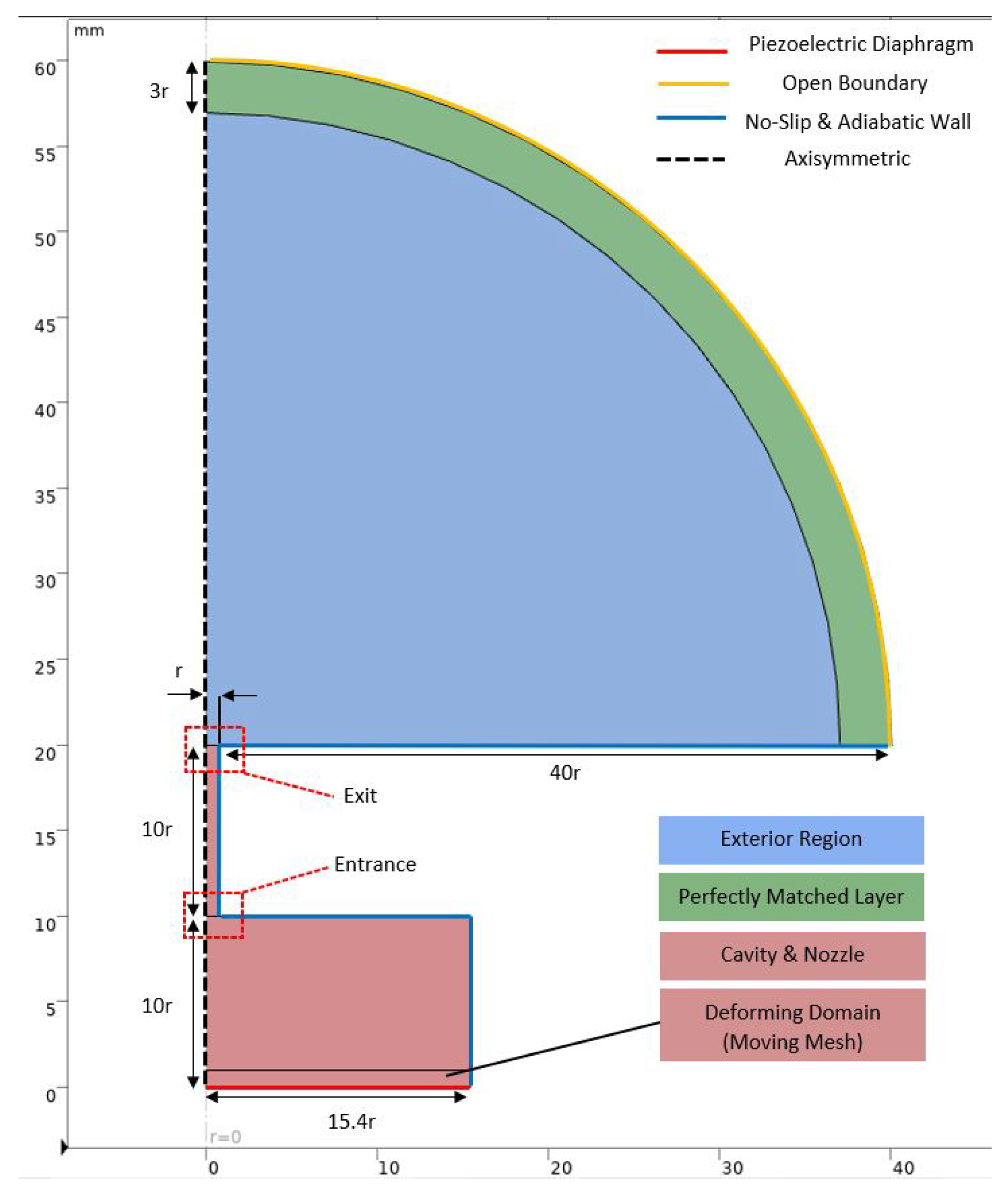
Figure 3.
Diaphragm Boundary Conditions.
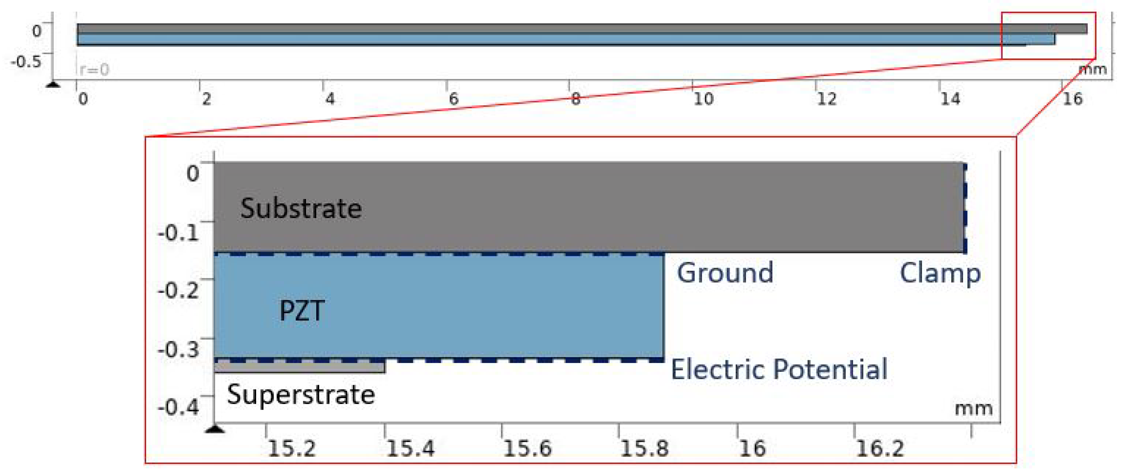
Figure 4.
Normalized displacement profiles of clamped diaphragm at its extreme positions.
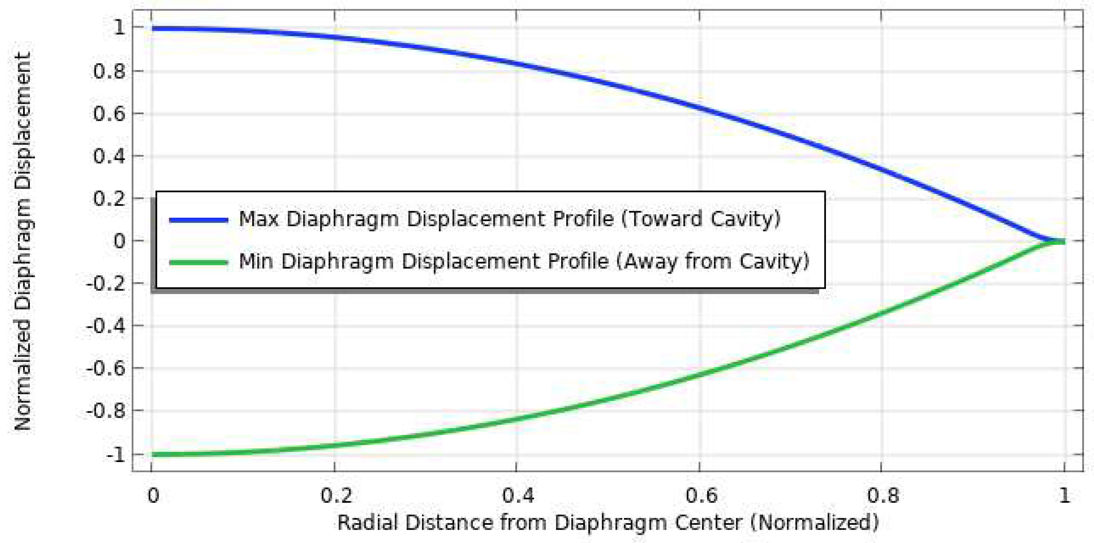
Figure 5.
Normalized diaphragm center displacement without voltage signal modification.
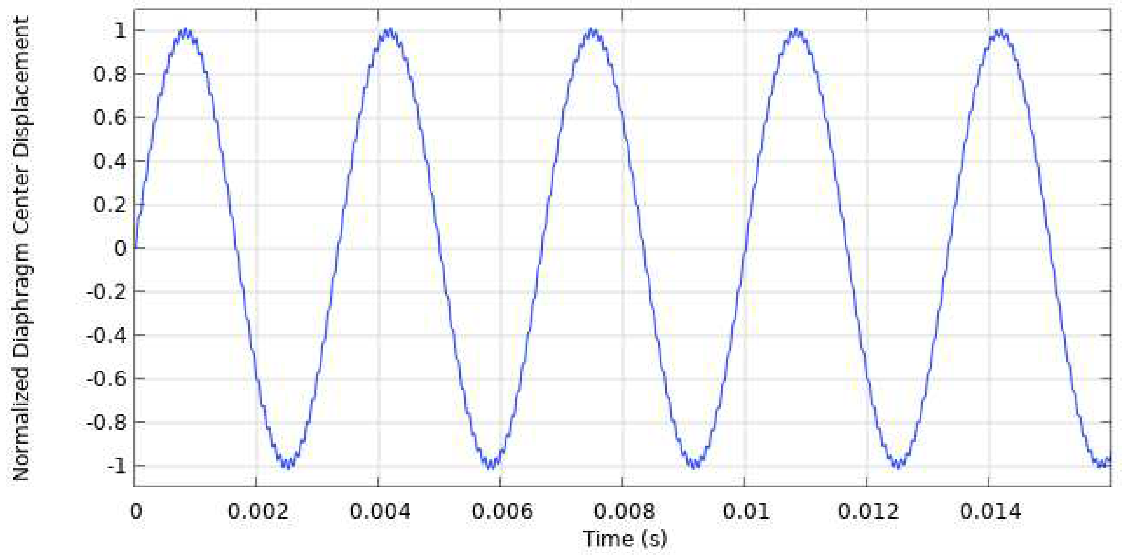
Figure 6.
Normalized diaphragm center displacement with voltage signal modification.
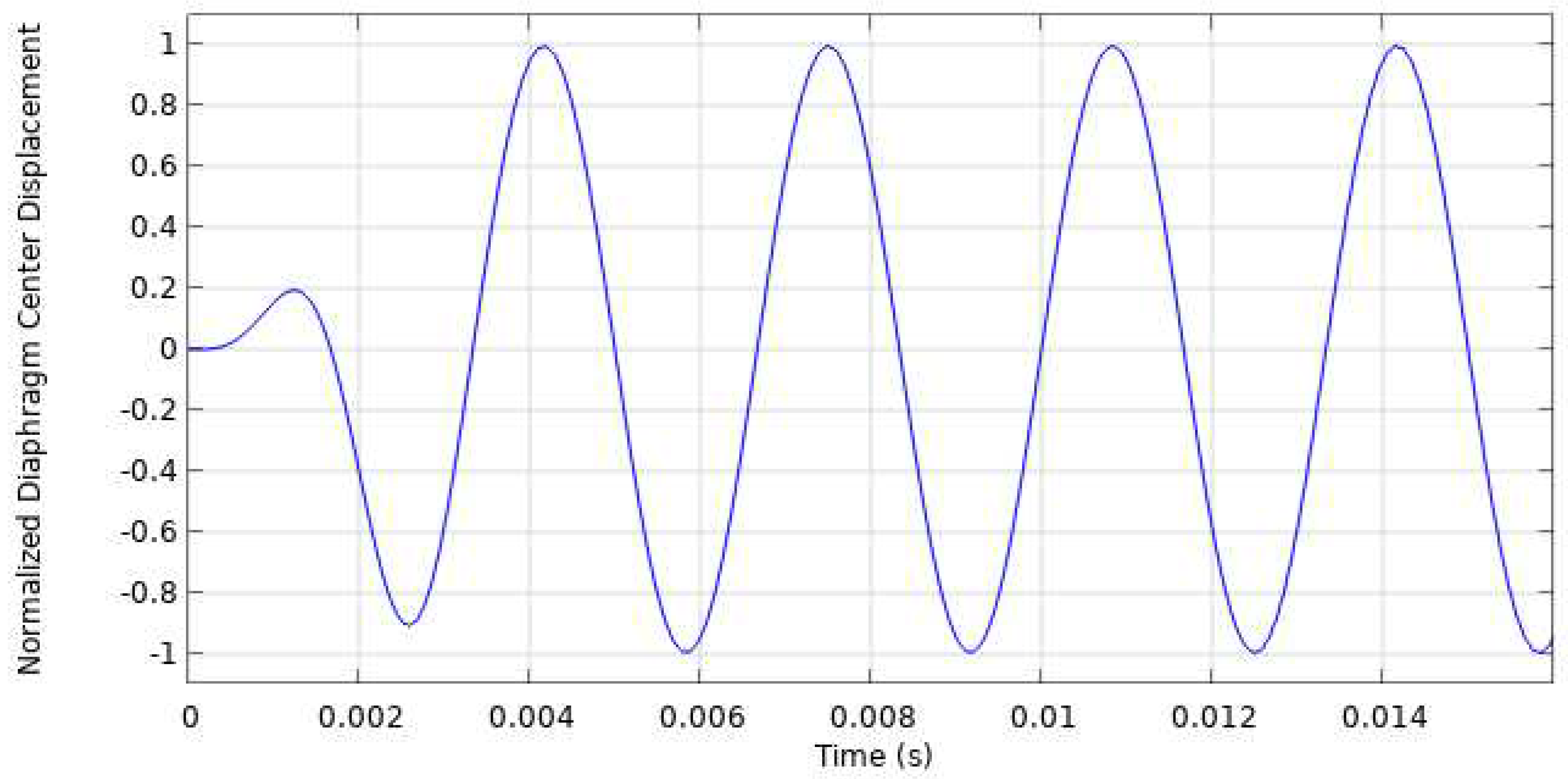
Figure 7.
Sound pressure level as a function of frequency at the nozzle exit and diaphragm surface.
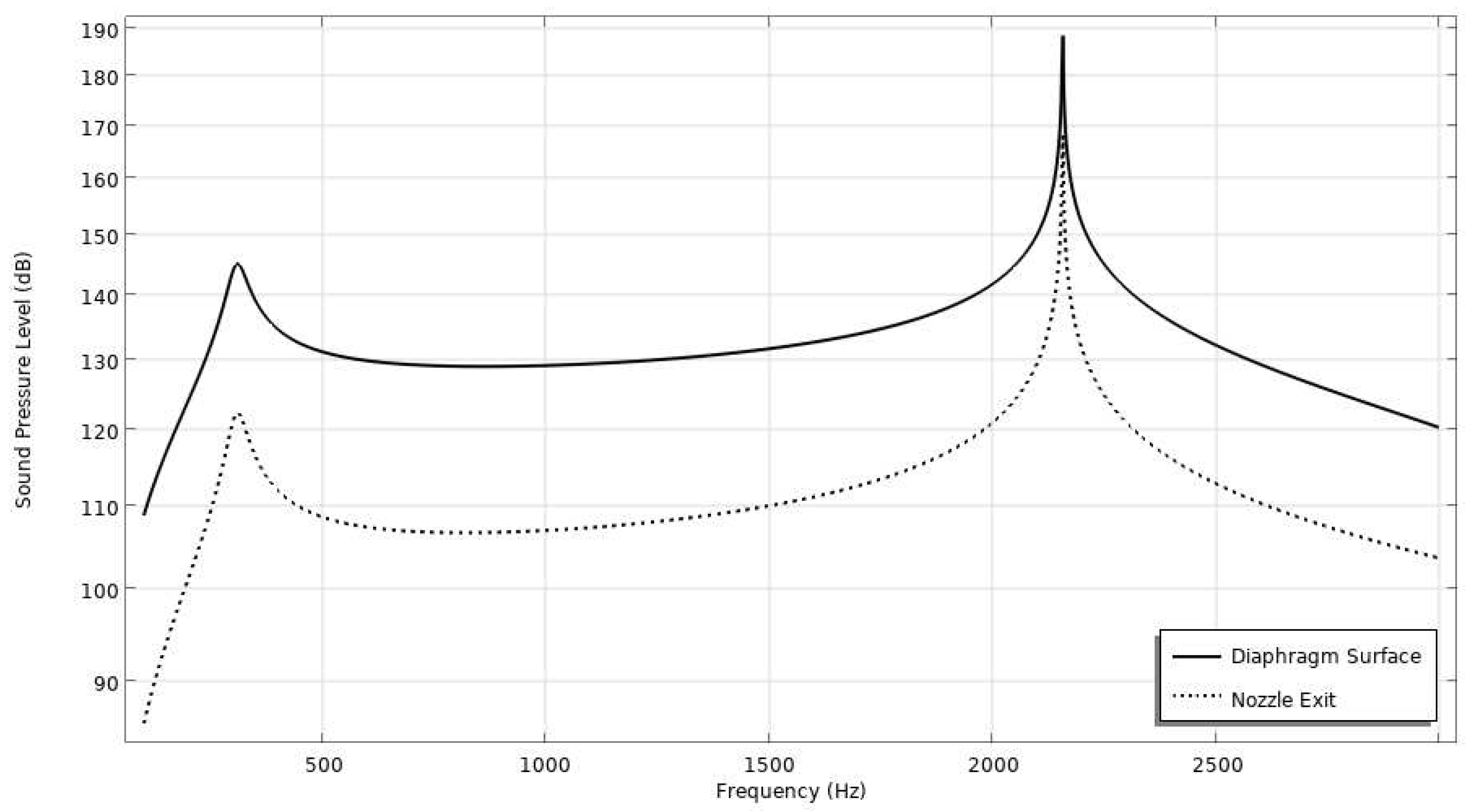
Figure 8.
2-D axisymmetric mesh with important regions highlighted.
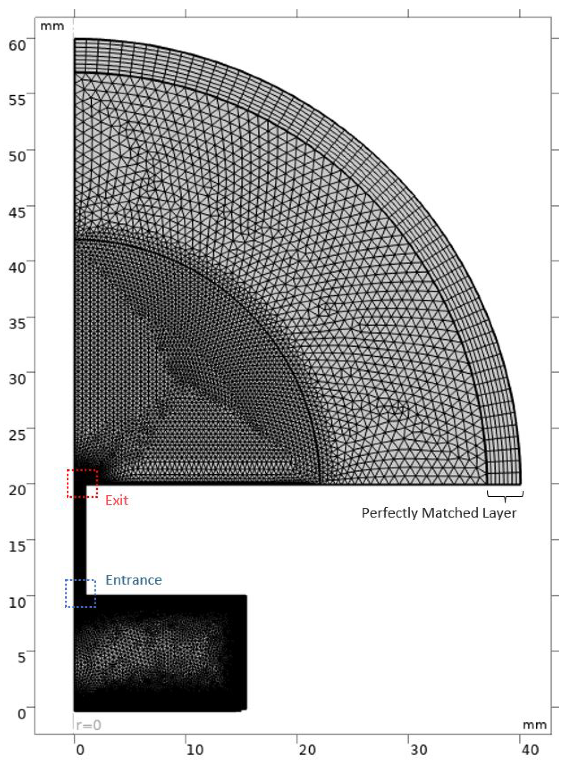
Figure 9.
Mesh at nozzle exit.
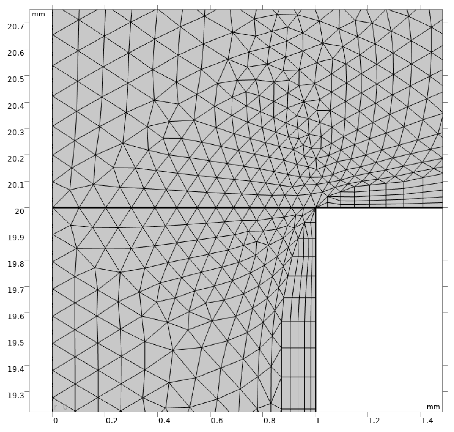
Figure 10.
Mesh at nozzle entrance.

Figure 11.
SJA nozzle exit centerline reaching steady state after a transient start-up condition.
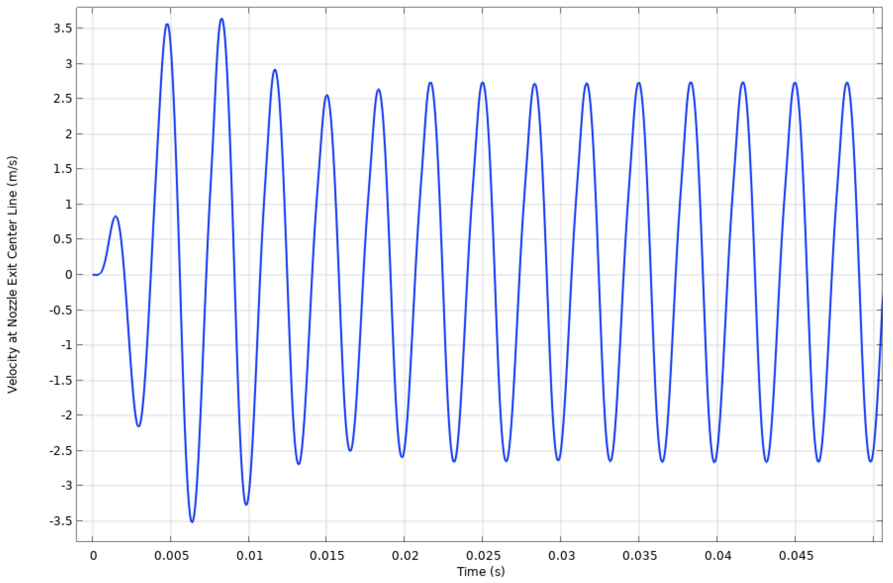
Figure 12.
Section of convergence plot during computation.
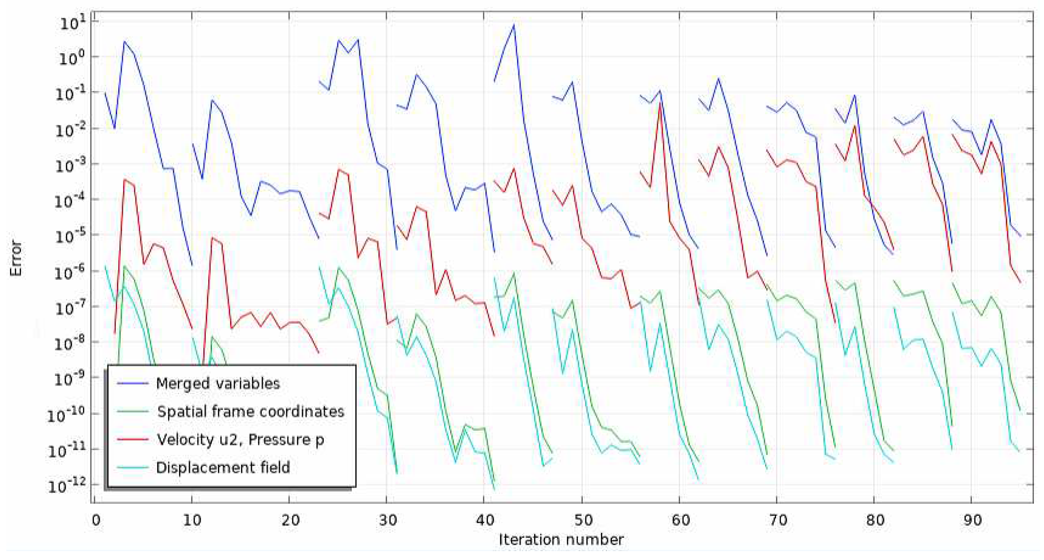
Figure 13.
Synthetic jet actuator centerline exit velocity response. Markers indicate experimental hot wire measurements [29] (blue ⋄) and the current multiphysics model (black □).
Figure 13.
Synthetic jet actuator centerline exit velocity response. Markers indicate experimental hot wire measurements [29] (blue ⋄) and the current multiphysics model (black □).
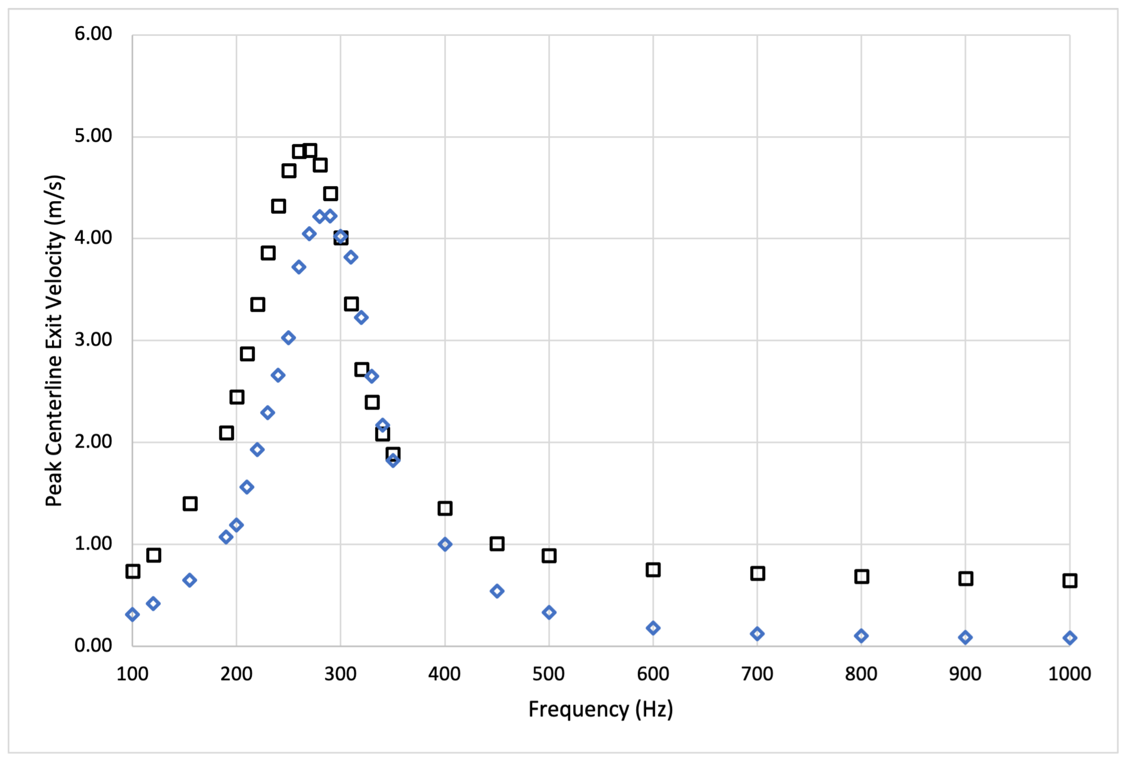
Figure 14.
Radial jet velocity profiles at SJA nozzle exit, normalized by maximum centerline velocity. Markers indicate hot wire [29] (red ∘), numerical [22] (blue ⋄), multiphysics (black □).
Figure 14.
Radial jet velocity profiles at SJA nozzle exit, normalized by maximum centerline velocity. Markers indicate hot wire [29] (red ∘), numerical [22] (blue ⋄), multiphysics (black □).

Figure 15.
Velocity magnitude contours for one cycle .
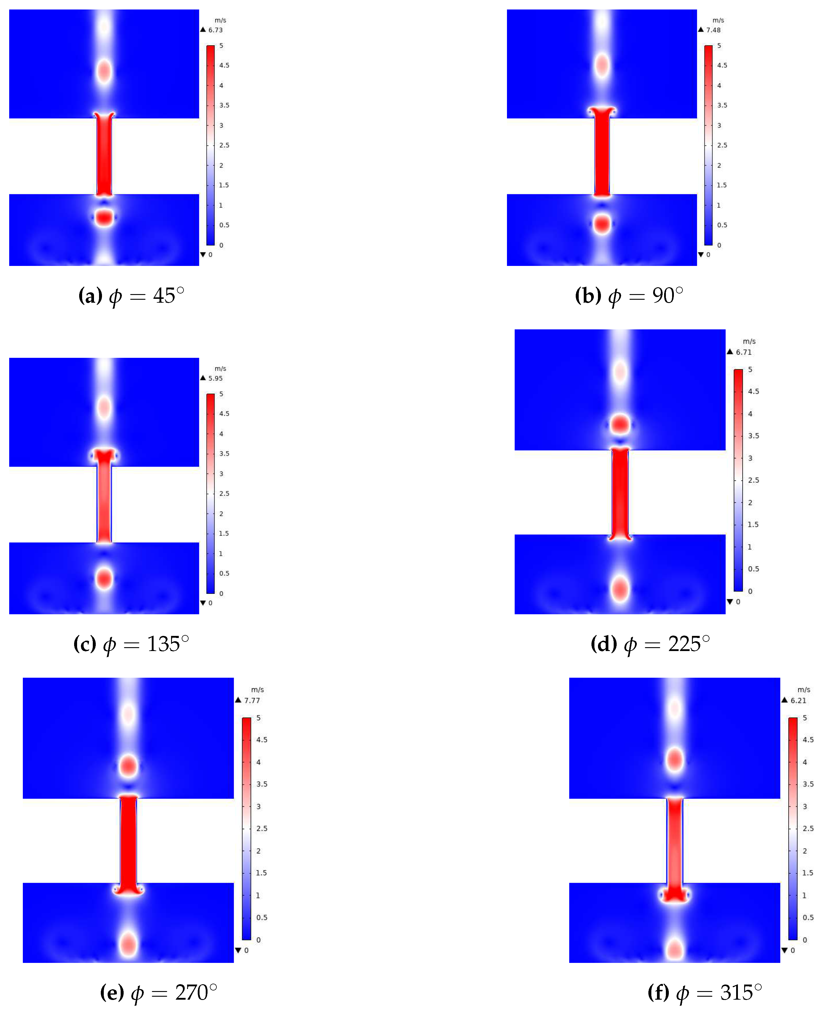
Figure 16.
Vorticity magnitude contours for one cycle of the multiphysics model.

Figure 17.
Normalized diaphragm and flow variables in response to a actuation frequency.
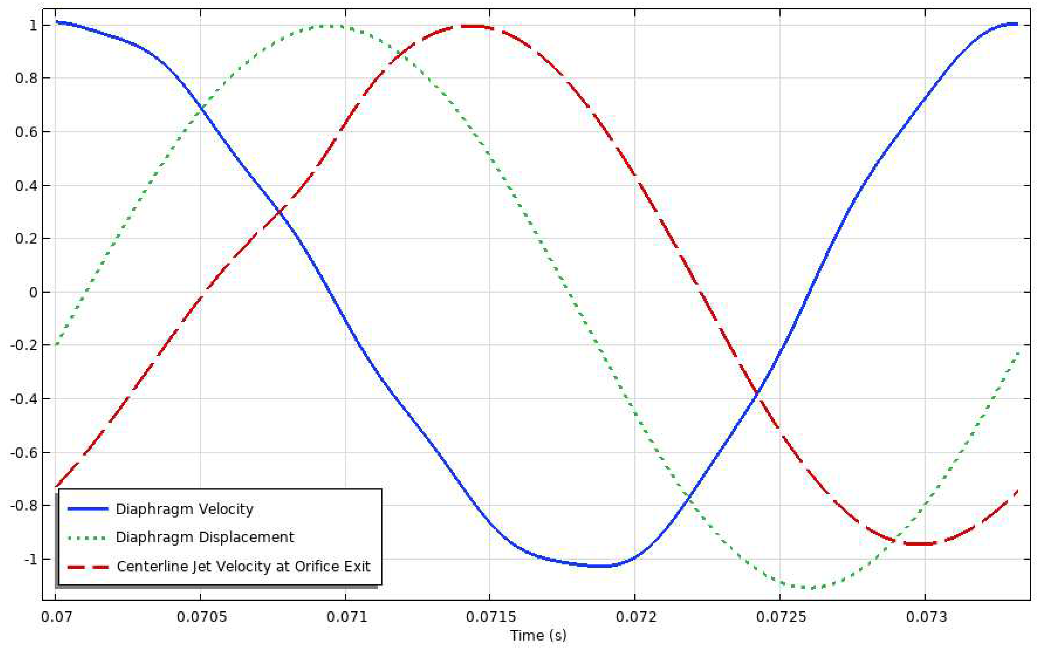
Figure 18.
Maximum acoustic pressure at the orifice exit as a function of actuation frequency. Markers indicate orifice exit centerline (blue ⋄) and diaphragm surface (black □).
Figure 18.
Maximum acoustic pressure at the orifice exit as a function of actuation frequency. Markers indicate orifice exit centerline (blue ⋄) and diaphragm surface (black □).
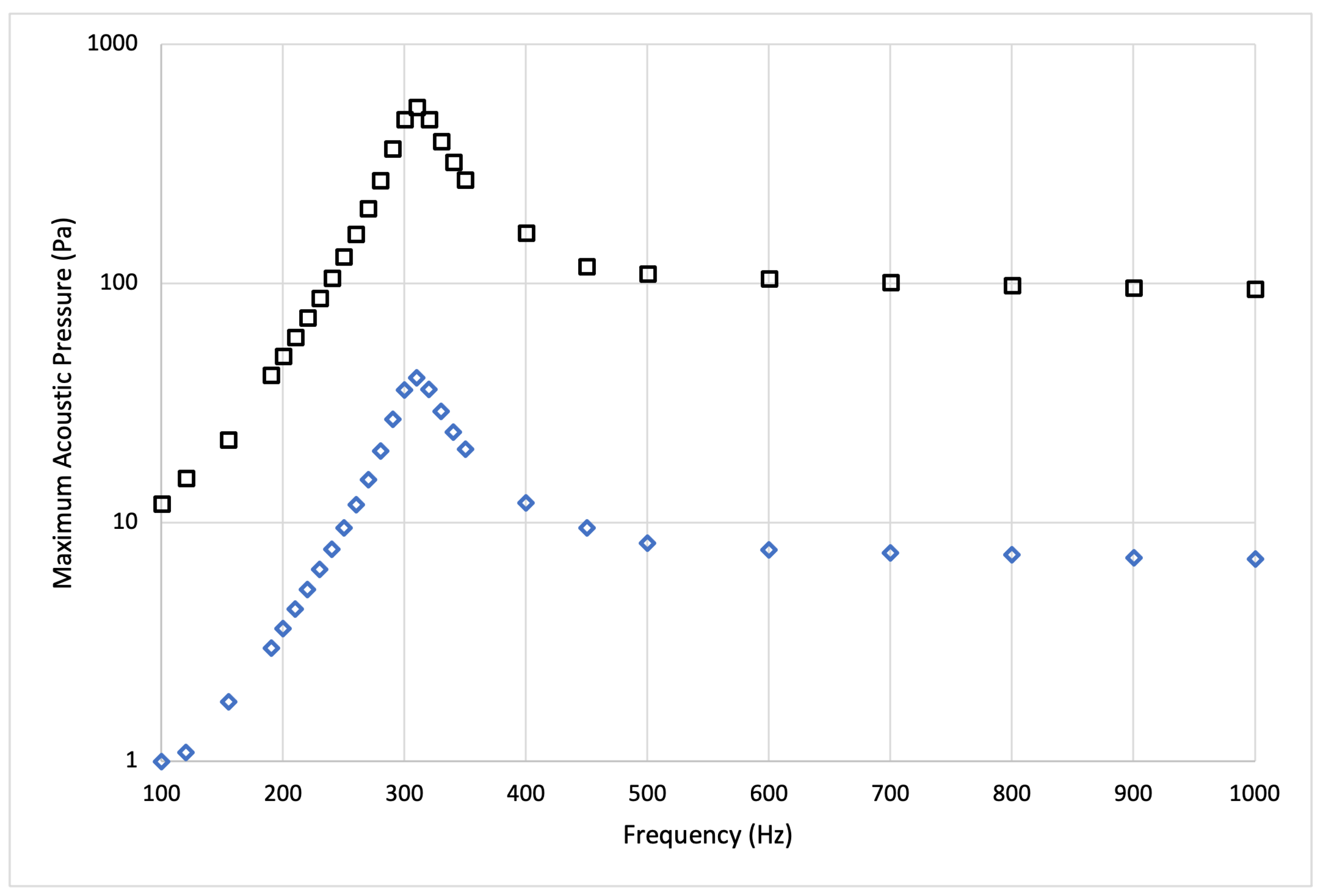
Figure 19.
Acoustic transient response of synthetic jet actuator at its orifice operating at without thermoviscous losses.
Figure 19.
Acoustic transient response of synthetic jet actuator at its orifice operating at without thermoviscous losses.

Figure 20.
Acoustic transient response of synthetic jet actuator at its orifice operating at without thermoviscous losses.
Figure 20.
Acoustic transient response of synthetic jet actuator at its orifice operating at without thermoviscous losses.
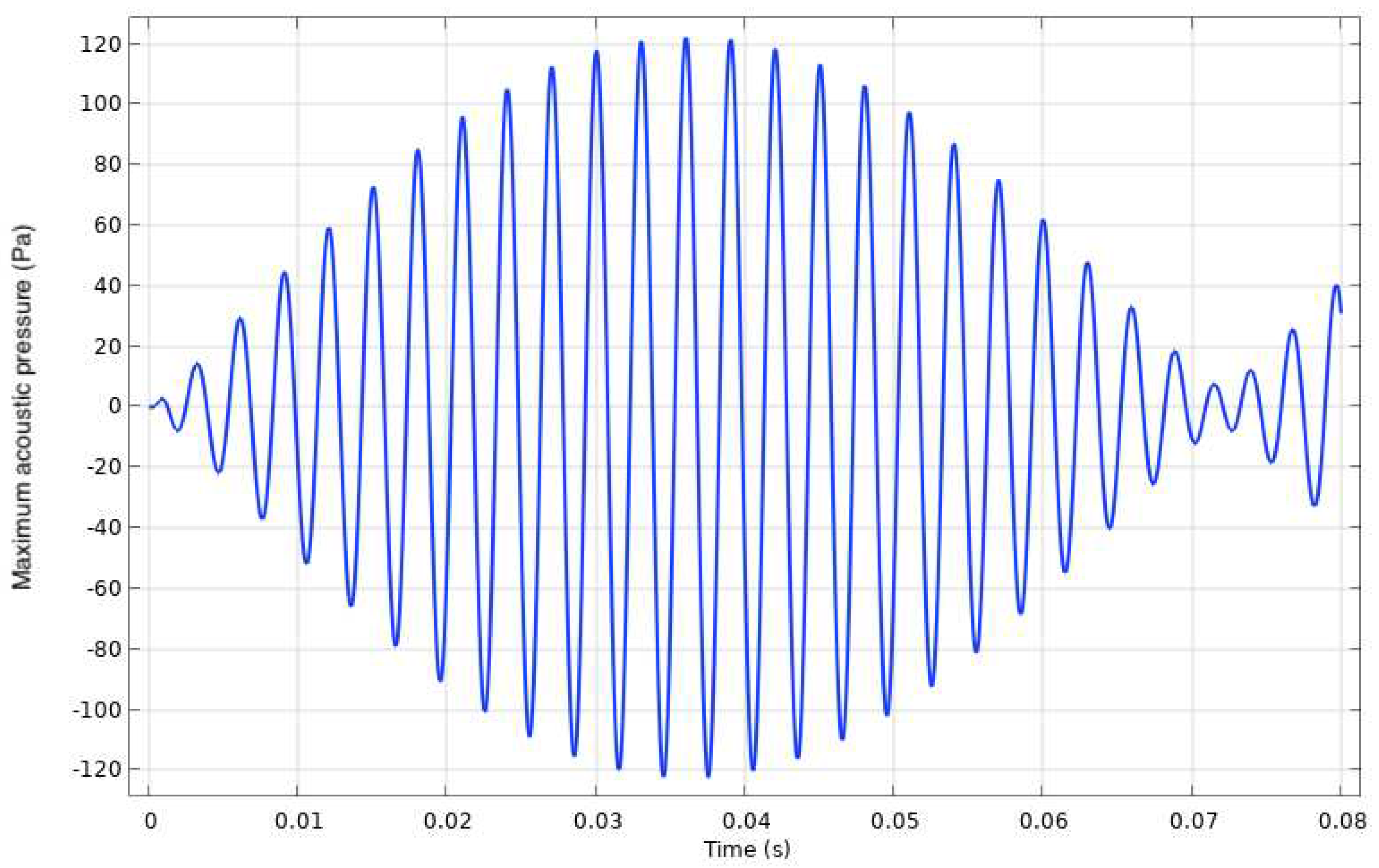
Figure 21.
Discrete Fourier transform of transient acoustic response of synthetic jet actuator operating at without thermoviscous losses.
Figure 21.
Discrete Fourier transform of transient acoustic response of synthetic jet actuator operating at without thermoviscous losses.
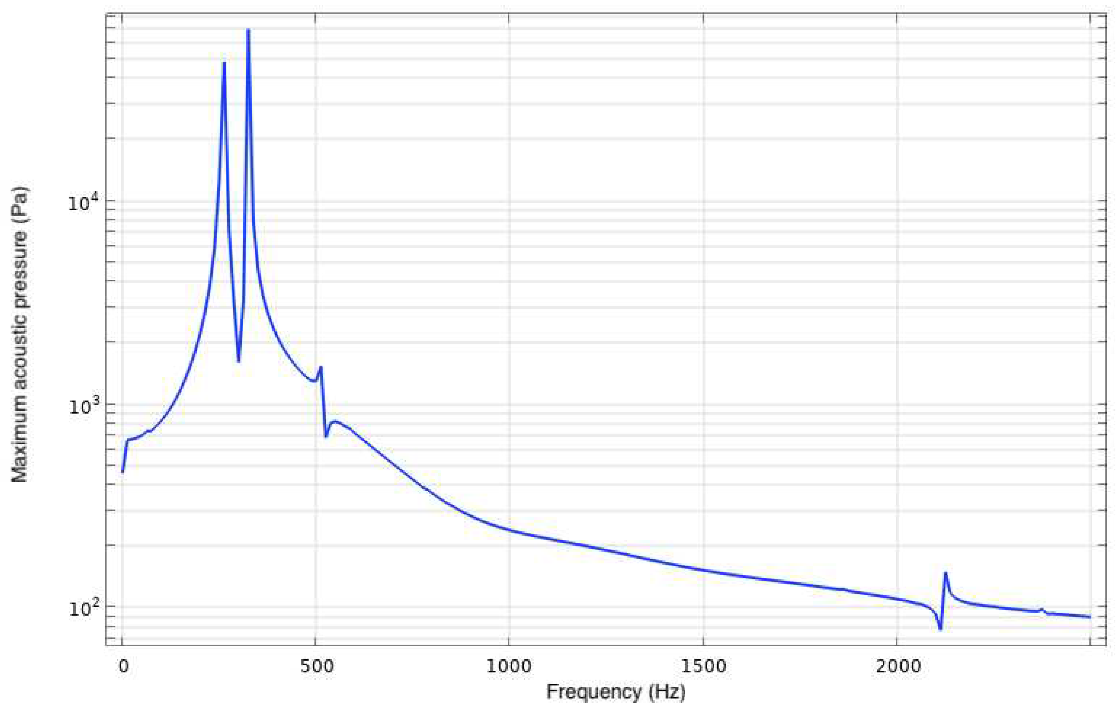
Figure 22.
Discrete Fourier transform of transient acoustic response of synthetic jet actuator operating at without thermoviscous losses.
Figure 22.
Discrete Fourier transform of transient acoustic response of synthetic jet actuator operating at without thermoviscous losses.
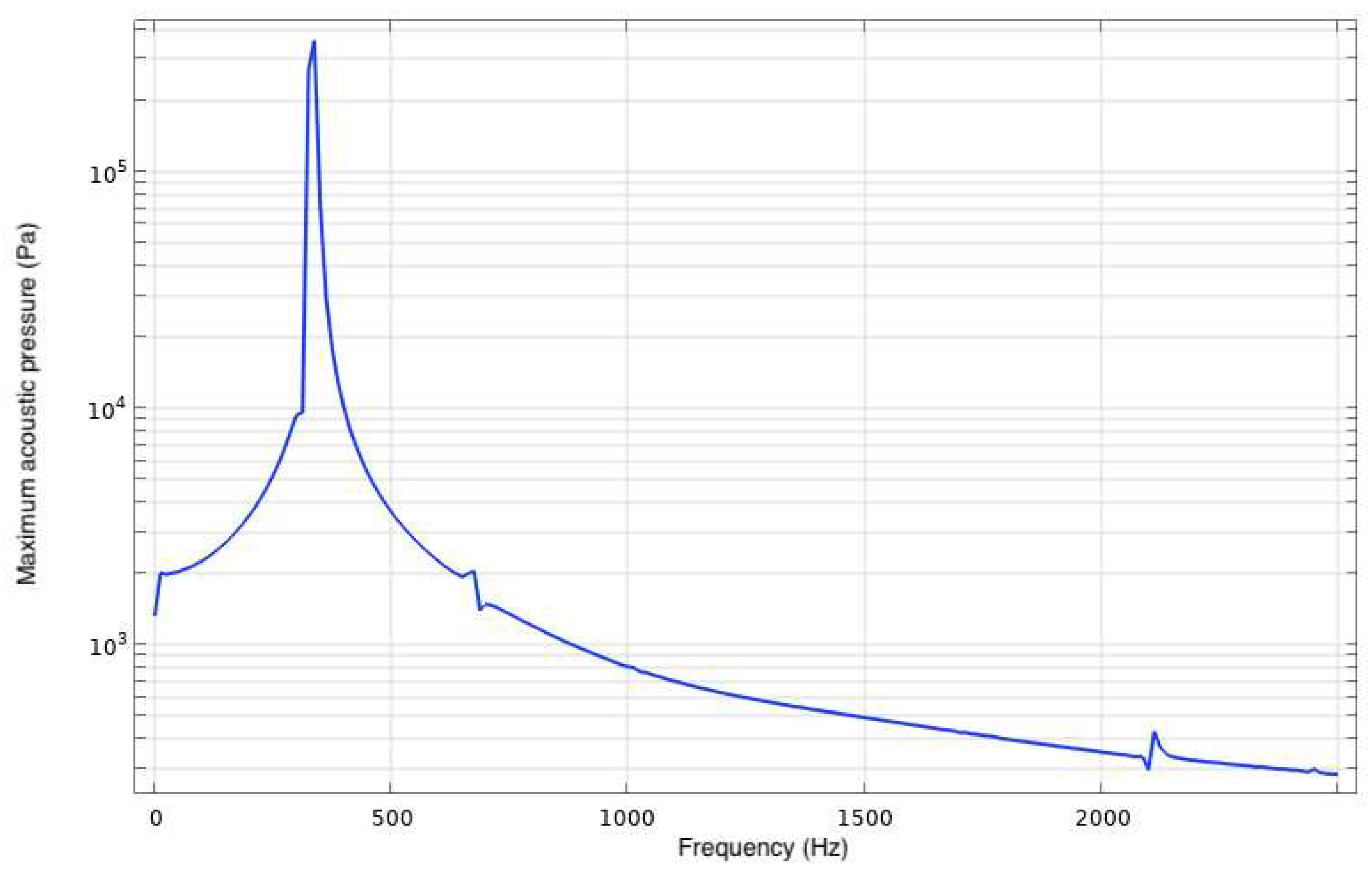
Figure 23.
Transient acoustic response of synthetic jet actuator operating at with thermoviscous losses.
Figure 23.
Transient acoustic response of synthetic jet actuator operating at with thermoviscous losses.
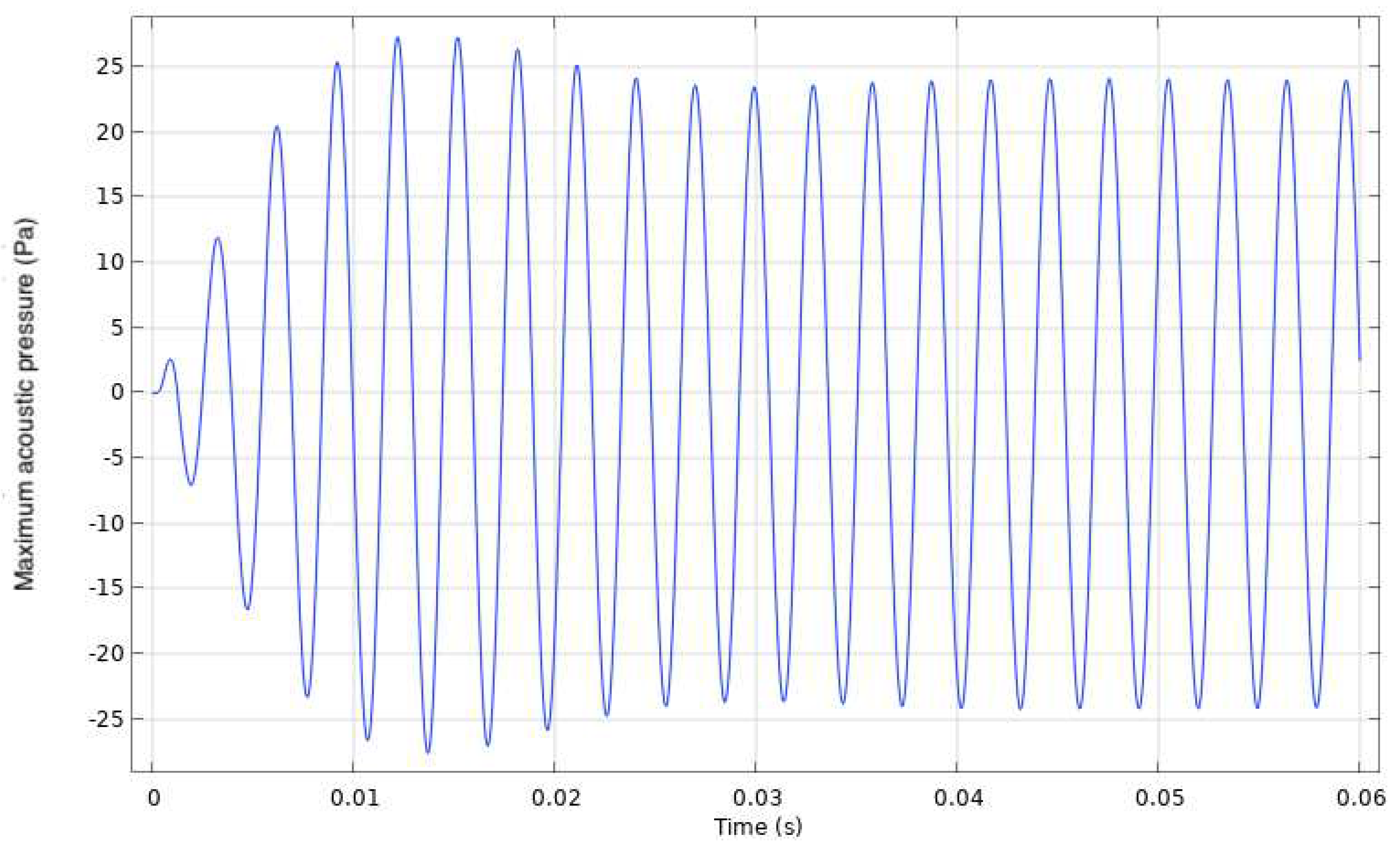
Figure 24.
Discrete Fourier transform of transient acoustic response of synthetic jet actuator operating at with thermoviscous losses.
Figure 24.
Discrete Fourier transform of transient acoustic response of synthetic jet actuator operating at with thermoviscous losses.
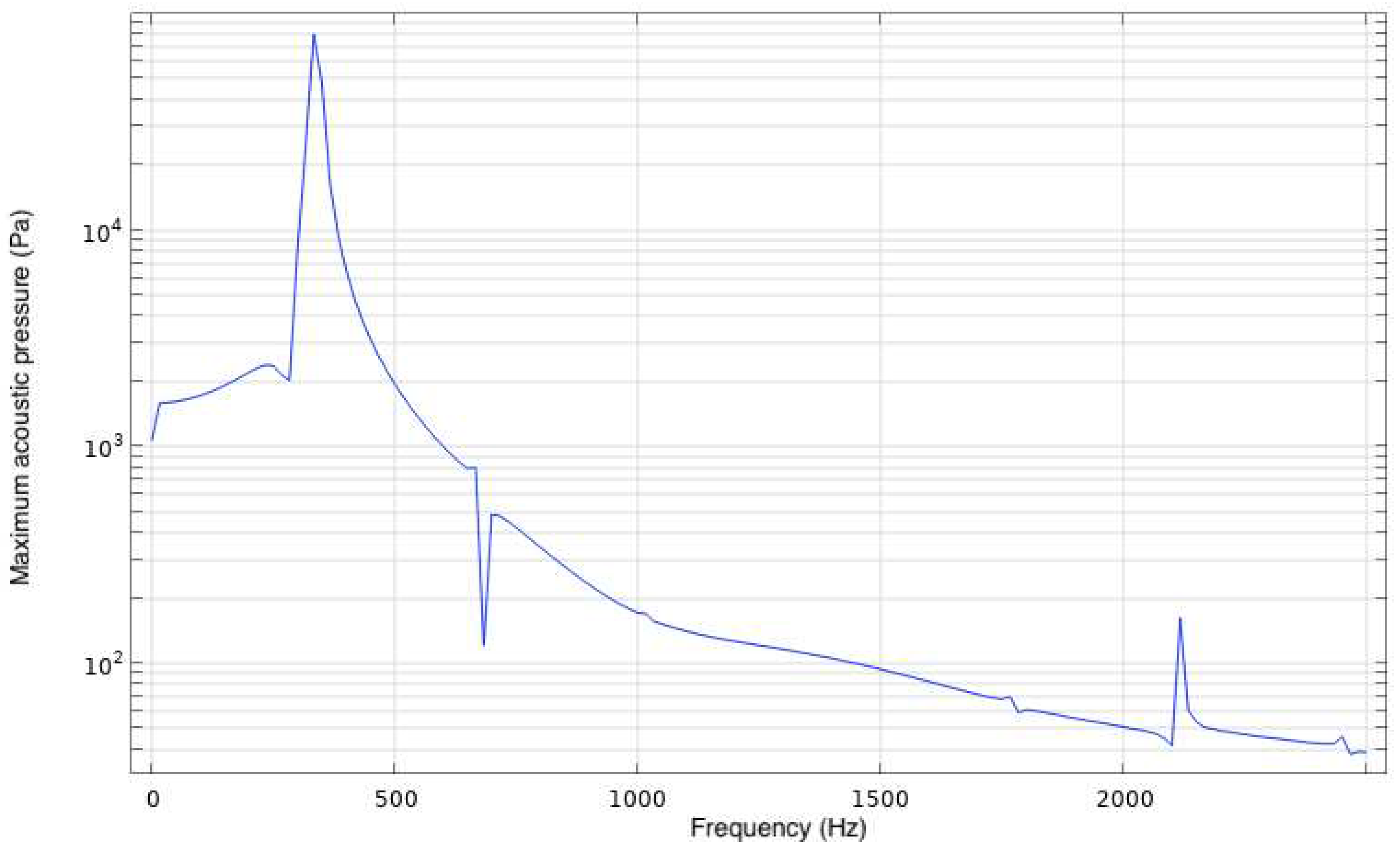
Figure 25.
Transient acoustic response of synthetic jet actuator operating at with thermoviscous losses.
Figure 25.
Transient acoustic response of synthetic jet actuator operating at with thermoviscous losses.
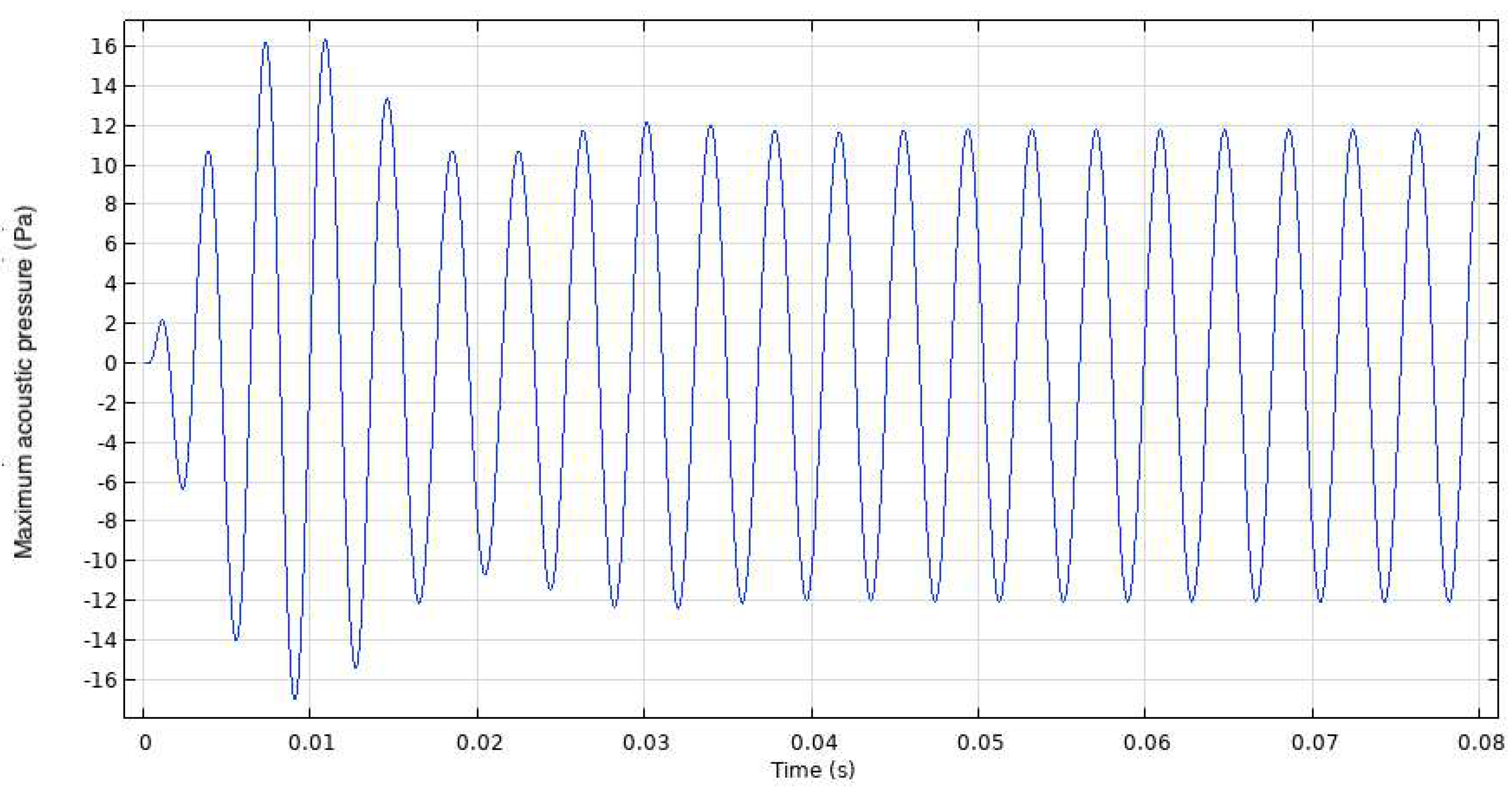
Figure 26.
Discrete Fourier transform of transient acoustic response of synthetic jet actuator operating at with thermoviscous losses.
Figure 26.
Discrete Fourier transform of transient acoustic response of synthetic jet actuator operating at with thermoviscous losses.
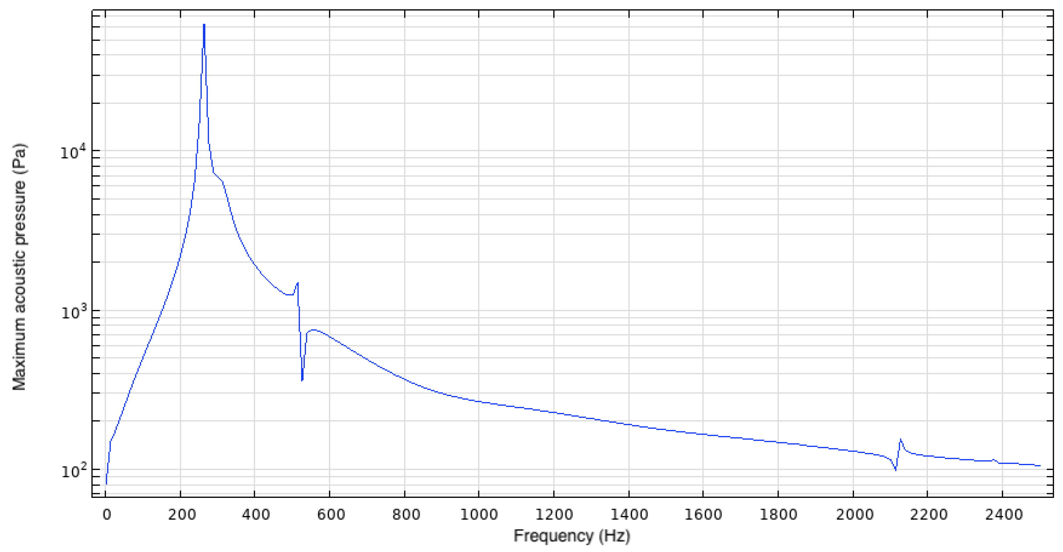
Figure 27.
A comparison of the many diaphragm treatments in the literature to the current multiphysics approach.
Figure 27.
A comparison of the many diaphragm treatments in the literature to the current multiphysics approach.
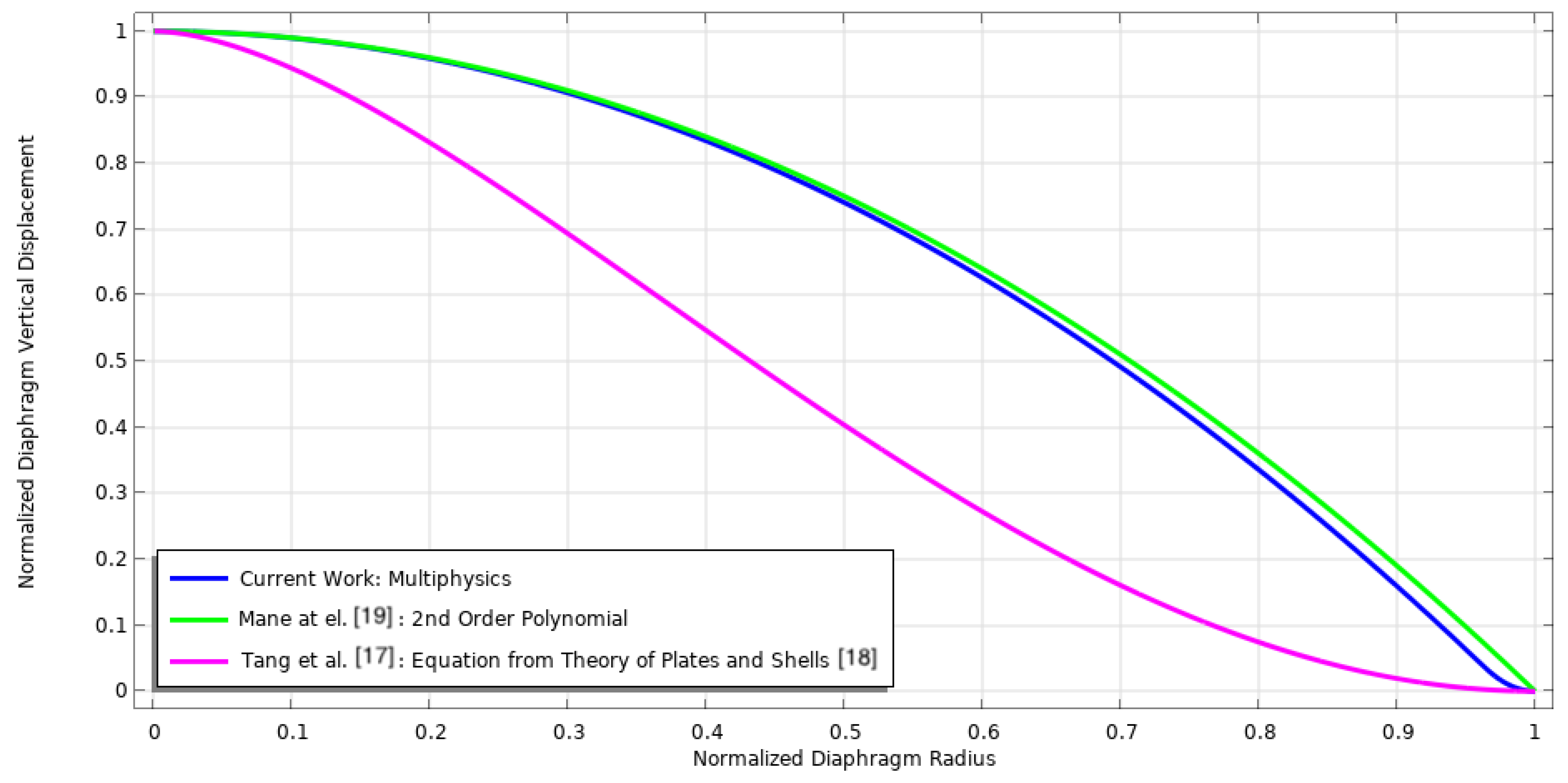
Figure 28.
The deflection profiles of the diaphragm at its highest and lowest point while operating at .
Figure 28.
The deflection profiles of the diaphragm at its highest and lowest point while operating at .


Table 1.
THUNDER TH-5C piezoelectric transducer material and geometric properties.
| Layer | Material | b (mm) | D (mm) | E (GPa) | ν |
| Substrate | Stainless Steel 302 | 0.1524 | 32.77 | 193 | 0.29 |
| Adhesive | LaRC-SI | 0.0381 | 31.75 | 3.8 | 0.4 |
| Piezoelectric | PZT-5A | 0.1905 | 31.75 | 63 | 0.31 |
| Adhesive | LaRC-SI | 0.0381 | 30.73 | 3.8 | 0.4 |
| Superstrate | Aluminum Alloy 2024 | 0.0254 | 30.73 | 69 | 0.33 |
Table 2.
PZT-5A elastic constants, (x).
| 12.03 | 7.52 | 7.51 | 0 | 0 | 0 |
| 7.52 | 12.03 | 7.51 | 0 | 0 | 0 |
| 7.51 | 7.51 | 11.09 | 0 | 0 | 0 |
| 0 | 0 | 0 | 2.11 | 0 | 0 |
| 0 | 0 | 0 | 0 | 2.11 | 0 |
| 0 | 0 | 0 | 0 | 0 | 2.26 |
Table 3.
PZT-5A piezoelectric constants, ().
| 0 | 0 | 0 | 0 | 12.29 | 0 |
| 0 | 0 | 0 | 12.29 | 0 | 0 |
| -5.35 | -5.35 | 15.78 | 0 | 0 | 0 |
Table 4.
Mesh sensitivity analysis of maximum displacement of THUNDER TH-5C actuator in response to 424 V load.
Table 4.
Mesh sensitivity analysis of maximum displacement of THUNDER TH-5C actuator in response to 424 V load.
| No. of Cells | 200 | 448 | 1070 | 2150 | 4565 | 9078 |
| Displacement (mm) | 0.1295 | 0.1297 | 0.1299 | 0.1301 | 0.1302 | 0.1302 |
Table 5.
Predicted Maximum Nozzle Centreline Exit Velocity for 2-D and 3-D Models.
| Excitation Frequency (Hz) | 270 | 285 | 300 | 310 |
| Max. Centreline Velocity: 2-D (m/s) | 3.98 | 4.33 | 4.42 | 3.80 |
| Max. Centreline Velocity: 3-D (m/s) | 4.02 | 4.39 | 4.49 | 3.85 |
Table 6.
Synthetic jet actuator characterization: location of centerline velocity peak associated with Helmholtz frequency.
Table 6.
Synthetic jet actuator characterization: location of centerline velocity peak associated with Helmholtz frequency.
| Theoretical | Model | Experiment | |
| Frequency (Hz) | 307.0 | 267.1 | 286.0 |
| Jet Velocity (m/s) | N/A | 5.05 | 4.25 |
Disclaimer/Publisher’s Note: The statements, opinions and data contained in all publications are solely those of the individual author(s) and contributor(s) and not of MDPI and/or the editor(s). MDPI and/or the editor(s) disclaim responsibility for any injury to people or property resulting from any ideas, methods, instructions or products referred to in the content. |
© 2023 by the authors. Licensee MDPI, Basel, Switzerland. This article is an open access article distributed under the terms and conditions of the Creative Commons Attribution (CC BY) license (http://creativecommons.org/licenses/by/4.0/).
Copyright: This open access article is published under a Creative Commons CC BY 4.0 license, which permit the free download, distribution, and reuse, provided that the author and preprint are cited in any reuse.


