Submitted:
29 December 2023
Posted:
29 December 2023
You are already at the latest version
Abstract
In this paper, we propose a method for assessing the effectiveness of entropy features using several chaotic mappings. We anlyze fuzzy entropy (FuzzyEn) and neural network entropy (NNetEn) on four discrete mappings: the logistic map, the sine map, the Planck map, and the two-memristor-based map, with a base length time series of 300 elements. FuzzyEn is shown to have improved global efficiency (GEFMCC) in the classification task compared to NNetEn. At the same time, there are local areas of the time series dynamics in which the classification efficiency NNetEn is higher than FuzzyEn. The results of using horizontal visibility graphs (HVG) instead of the raw time series are also shown. GEFMCC decreases after HVG time series transformation, but there are local areas of the time series dynamics in which the classification efficiency increases after including the HVG. The scientific community can use the results to explore the efficiency of entropy-based classification of time series.
Keywords:
chaotic maps
; NNetEn
; neural network entropy
; horizontal visibility graphs
; fuzzy entropy
; classification
; entropy global efficiency
; GEFMCC
MSC: 37M10; 54C70; 68T01
1. Introduction
Classification of time series based on entropy analysis and machine learning (ML) is a trending task in studying nonlinear signals. For example, EEG classification in diagnosing Alzheimer's disease [1,2] and Parkinson's disease [3,4,5,6]. There are many types of entropies, which in turn have several customizable parameters, for example, sample entropy (SampEn) [7], cosine similarity entropy (CoSiEn) [8], singular value decomposition entropy (SVDEn) [9], fuzzy entropy (FuzzyEn) [10], permutation entropy (PermEn) [11], etc. In this context, it is a problem of paramount importance to assess the effectiveness of the different entropies when used as features in ML classification. Recently, Velichko et al. proposed the use of a LogNNet neural network [12,13] for neural network entropy (NNetEn) calculation [1]. LogNNet neural network is a feedforward neural network that uses filters based on the logistic function and a reservoir inspired by recurrent neural networks, thus enabling the transformation of a signal into a high-dimensional space. Its efficiency was validated on the MNIST-10 data set [14]. They showed that the classification performance is proportional to the entropy of the time series and has a stronger correlation than the Lyapunov exponent of the time series used to feed the reservoir. The effectiveness of using NNetEn was shown on EEG signals in diagnosing Alzheimer's disease [1]. The effectiveness of fuzzy entropy was also demonstrated in the paper of Belyaev et al. [3] in diagnosing Parkinson's disease.
Natural visibility graph (NVG) graphs were introduced in [15] as a simple and computationally efficient method to represent a time series as a graph. Visibility graphs preserve the periodic and chaotic properties of the discrete map [15] , see also [16,17,18]. For example, periodic series result in regular graphs, random series in random graphs, and fractal series in scale-free graphs. Horizontal Visibility Graphs (HVG) were introduced in [19] to simplify the previously described NVG. Visibility graphs (VG) enable to reduce the complexity of calculations which depend on time series, while preserving the accuracy on the results, see for instance [20,21,22]
In [23], the authors describe the advantages of using the amplitude difference distribution instead of the degree distribution to collect information from the network formed by the horizontal visibility graph. Li and Shang introduce a combination of the amplitude difference distribution with discrete generalized past entropy to present a new method called Discrete Generalized Past Entropy based on the Amplitude Difference Distribution of the Horizontal Visibility Graph (AHVG-DGPE). The authors note its efficiency in systems evaluation and higher accuracy and sensitivity rate compared to the traditional method in characterizing dynamic systems, see also [24,25,26]
In this paper, we propose a method for assessing the effectiveness of entropies using chaotic mappings: We use it for analyzing the FuzzyEn and NNetEn entropies on four discrete mappings is given: the logistic map, the sine map, the Planck map, and the two-memristor based map. We use the corresponding HVG degrees representation of these time series, which implies that the resulting time series does not consist of real numbers but only of integer numbers. The results of using horizontal visibility graphs (HVG) to classify time series are also shown:
The major contributions of the paper are:
- A concept for comparing the efficiency of classifying chaotic time series using entropy features is presented.
- A new characteristic for assessing the global efficiency of entropy (GEFMCC) is presented.
- A comparison of the effectiveness of FuzzyEn and NNetEn was investigated. FuzzyEn is shown to have improved GEFMCC in the classification task compared to NNetEn. At the same time, there are local areas of the time series dynamics in which the classification efficiency NNetEn is higher than FuzzyEn. Matthews correlation coefficient was used to evaluate binary classification.
- The results of using HVG are shown. GEFMCC decreases after HVG time series transformation, but there are local areas of the time series dynamics in which the classification efficiency increases after HVG.
2. Materials and Methods
2.1. Generation of synthetic time series
To generate synthetic time series, we used several types of the discrete chaotic map. The control parameter rj (j = 1...Nr) varied discretely with step dr.

2. Sine map [29]:

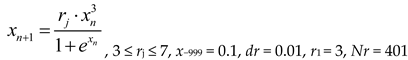
3. Planck map [30]:
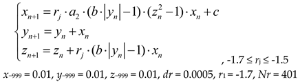
4. Two-memristor based map (TMBM) [31]:
The first 1,000 elements (x-999…x0) are ignored due to the transient period. If n > 0, then the time series is calculated for xn. To generate a class corresponding to one value of rj, 100-time series were generated with a length of N = 300 elements. Elements in each series were calculated sequentially, (x1, …, x300), (x301, ..., x600), etc. A set of 100 time series was generated at a given rj. The value rj ran through the entire range with a certain step dr, see equations (1-4).
2.2. Natural and Horizontal Visibility Graphs
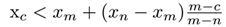
Given a time series {(n,xn)}n∈ℕ indexed on the set of natural numbers ℕ, such that at time n the time series takes the value xn, an association between each node and each pair (n, xn) in order to obtain the graph associated to the time series. A natural visibility graph (NVG) is constructed as follows: given two nodes (n,xn) and (m, xm), these two nodes have visibility and thus they are connected in the graph by an edge if any other pair (c, xc) with n < c < m satisfies
Horizontal Visibility Graphs (HVG) were introduced in [19,32] to simplify the requirements described for NVG.
When computing the HVG, each time series value is related a node in the resulting graph, as in the case of NVG. Two nodes (n, xn) and (m, xm) in this graph are connected if a horizontal line can be drawn connecting their corresponding visibility index without intersecting any intermediate value that is, if xn, xm > xc for all n < c < m, see the examples in Figure 1.
Python library ts2vg was used to calculate HVG (‘time series to visibility graphs’) [33], which implements algorithms for plotting graphs based on time series data. The package utilizes a highly effective C backend for its operations (using Cython) and seamlessly integrates with the Python environment. As a result, ts2vg can effortlessly process input data from various sources using established Python tools. Additionally, it enables the examination and interpretation of the generated visibility graphs using a wide range of graph analysis, data science, visualization packages and tools compatible with Python. The HorizontalVG method was used to construct the HVG.
2.3. Time series classification metrics
We describe the method for calculating the classification metric for the time series of a discrete map for neighboring sets corresponding to two neighboring partitions by r.
Figure 2a shows a section of the buffering diagram of the logistic mapping with two adjacent sets of series corresponding to rj-1 = 3.634 and rj = 3.636; the distance between them corresponds to dr. Each set contains 100 time series. Examples of the first time series (x1, …, x300) for each set are shown in Figure 2b,c. FuzzyEn values for 100 time series in each set are shown in Figure 2d. We denote the average entropy value in each set as Entropy_AV (FuzzyEn_AV or NNetEn_AV).
As a result, we compiled a database with two classes. Class 1 contains 100 entropy values of time series generated at rj = 3.636, and Class 2 contains 100 entropy values of time series generated at rj-1 = 3.634. To classify the two classes, we will use the threshold model.
The single feature threshold approach involves a simple ML model with a single threshold Vth separating the two classes. A formula can represent the separation algorithm.
The search for Vth was carried out by sequential search within the limits of changes in the entropy feature, with the determination of the maximum MCC (Matthews correlation coefficient [34]) value. We calculated MCC for the entire database without dividing it into test and training data, which is equivalent to calculating MCC on training data.
MCC is the correlation coefficient between observed and predicted classifications; it returns a value between -1 and +1. A coefficient of +1 represents a perfect prediction, 0 is a random prediction, and -1 indicates the opposite, inverted prediction. The higher the MCC module is, the more accurate the prediction is, too. A negative MCC value means that the classes must be swapped. The MCC is calculated using the values of the confusion matrix as [34].
where TP stands for (True Positive), TN for (True Negative), FP for (False Positive), and FN for (False Negative). The MCC metric is a popular metric in machine learning, including binary classification.
Figure 2d shows an example where the classes are well separable and MCC = 1. Figure 3 shows an example of entropy distribution for classes with rj-1 = 3.688 and rj = 3.69. It can be seen that the classes are poorly separable and MCC ~ 0.45.
The MCC(rj) dependence was calculated for all neighboring rj-1 and rj within the range of changes in r of each mapping j = 2…Nr. Let us introduce the concept of global efficiency (GEFMCC), which is calculated within the entire mapping under study using the formula
where j = 2…Nr is the index of partition by r, Nr is the maximum number of partitions, see equations (1-4). The GEFMCC characteristic is equivalent to the average value of the dependence modulus MCC(rj), and estimates the degree of entropy efficiency over the entire variety of time series of the chaotic mapping.
2.4. FuzzyEn calculation
FuzzyEn measures entropy based on fuzzily defined exponential functions for comparison of vectors similarity. It differs from approximate entropy and sample entropy, which use Heaviside function to calculate the irregularities in a time series data [35]. Fuzzy entropy can be calculated as follows. For a given time series with given embedding dimension , an as a form as:
These vectors represent consecutive values, starting with point, with the baseline removed. Then, the distance between vectors and , can be defined as the maximum absolute difference between their scalar components. Given and , the degree of similarity of the vectors and is calculated using fuzzy function.
The function is defined as:
Repeating the same procedure from equation (9-10) for the dimension to , vectors are formed and the function is obtained. Therefore, FuzzyEn can be estimated as:
In the computation of fuzzy entropy, the embedding dimension and tolerance r = 0.2 x std were used in the analysis, where std is a standard deviation of , argument exponent (pre-division) r2 = 3 and time delay .
2.5. NNetEn сalculation
Figure 4 shows the process for calculating NNetEn [1], it involves several key steps, which are detailed below:
Step 1: The initial step encompasses inputting the time series X = (x1…xN) of length N, into the reservoir.
Six main methods for filling the reservoir are researched in detail, as outlined in [36]. The methods M1 to M6 involve various techniques for filling the reservoir. M1—Row-wise filling with duplication; M2—Row-wise filling with an additional zero element; M3—Row-wise filling with time series stretching; M4—Column-wise filling with duplication; M5—Column-wise filling with an additional zero element; M6—Column-wise filling with time series stretching.
Step 2: Selection of embedded Datasets 1 and 2, upon which of the classification metric will be computed.
Step 3: Formation of the Y vector from the dataset, with the inclusion of a zero offset Y[0] = 1.
Step 4: Normalization of the Y vector.
Step 5: Multiplication of the Y vector with the reservoir matrix and the input vector Sh = W × Y to convert it into Sh vector.
Step 6: Feeding vector Sh into the input layer of the classifier, with a dimension of P_max = 25.
Step 7: Normalization of the vector Sh.
Step 8: Utilization of a single-layer output classifier.
Step 9 to 10: The neural network is trained according to backpropagation method with a variable number of epochs (Ep) and then tested. The parameter of the entropy function is referred as Ep.
Step 11: Transformation of the classification metric into the NNetEn entropy.
The parameters used in this work to calculate the entropy of NNetEn are: MNIST database data set (database = 'D1' and mu = 1), method for forming a reservoir from the M3 time series (method = 3), number of neural network training epochs (epoch) = 5 and the accuracy metric ('Acc').
3. Results
We present the results of calculating the dependencies between the FuzzyEn_AV(r) and NNetEn_AV(r) for various discrete mappings before and after the HVG transformation of the time series. In this way, we observe if visibility graphs retain enough information from the time series in order to calculate the entropies. The results of calculating the MCC(r) dependencies from which the characteristic of the global efficiency of GEFMCC from (8) is calculated are presented.
3.1 Results for logistic, sin and Planck maps
Figure 5a shows an example of a bifurcation diagram for a logistic map in the range of the control parameter 3.4 ≤ r ≤ 4, with a sampling step dr = 0.002. Figure 5b shows the FuzzyEn_AV(r) dependences before and after applying the HVG transformation. We can see that the HVG transformation leads to a significant increase in the entropy value, while some areas change their relative position. In regions A and B, we have reduced the entropies after having computed the HVGs, which is natural since they consist of ordered time series. The relative position of area C remains unchanged. The application of the HVG transformation has virtually no effect on the shape of the NNetEn_AV(r) graph, causing only a slight upward shift of entropies. The increase in FuzzyEn and NNetE values after HVG is due to the fact, in our opinion, that HVG has filtering properties and reduces the constant components of time series. However, FuzzyEn and NNetEn are sensitive to the constant component of the time series, which can be seen, for example, from the entropy values for r < 3.45.
Figure 6a shows the MCC(r) dependences for FuzzyEn before and after HVG transformation, as well as their difference ΔMCC, which is computed as follows:
Positive values of ΔMCC > 0 indicate that, for a given value of r, the degree of classification of time series for rj-1 and rj increases due to the HVG transformation. Conversely, negative ΔMCC values indicate a decrease in classification efficiency after HVG transformation. According to the lower figure, we see that the HVG transformation can lead to both an increase and a decrease in classification efficiency for different rj. We provide detailed calculations of the GEFMCC values in Table 1.
Figure 6b shows the MCC(r) dependences for NeNetEn before and after HVG transformation, and their difference ΔMCC. It can be seen that the amplitude of MCC for FuzzyEn is more significant than for NNetEn, which also affects the GEFMCC value in Table 1.
It is convenient to compare the local values of MCC(r) for FuzzyEn and NeNetEn using their difference ΔMCC (Figure 7).
Figure 7 shows local areas of the dynamics of time series in which the classification efficiency NNetEn is higher than FuzzyEn (ΔMCC > 0), but most of the graph has ΔMCC < 0.
Similar results were obtained for the sine and Planck maps. Figure A1a (Appendix A) shows an example of a bifurcation diagram for a sin map in the control parameter range 0.7 ≤ r ≤ 2, with a sampling step dr = 0.005. Figure A1b,c shows the FuzzyEn_AV(r) and NNetEn_AV(r) dependences before and after applying the HVG transformation. Figure A2 shows the MCC(r) dependences for FuzzyEn and NNetEn before and after HVG transformation, and their difference ΔMCC.
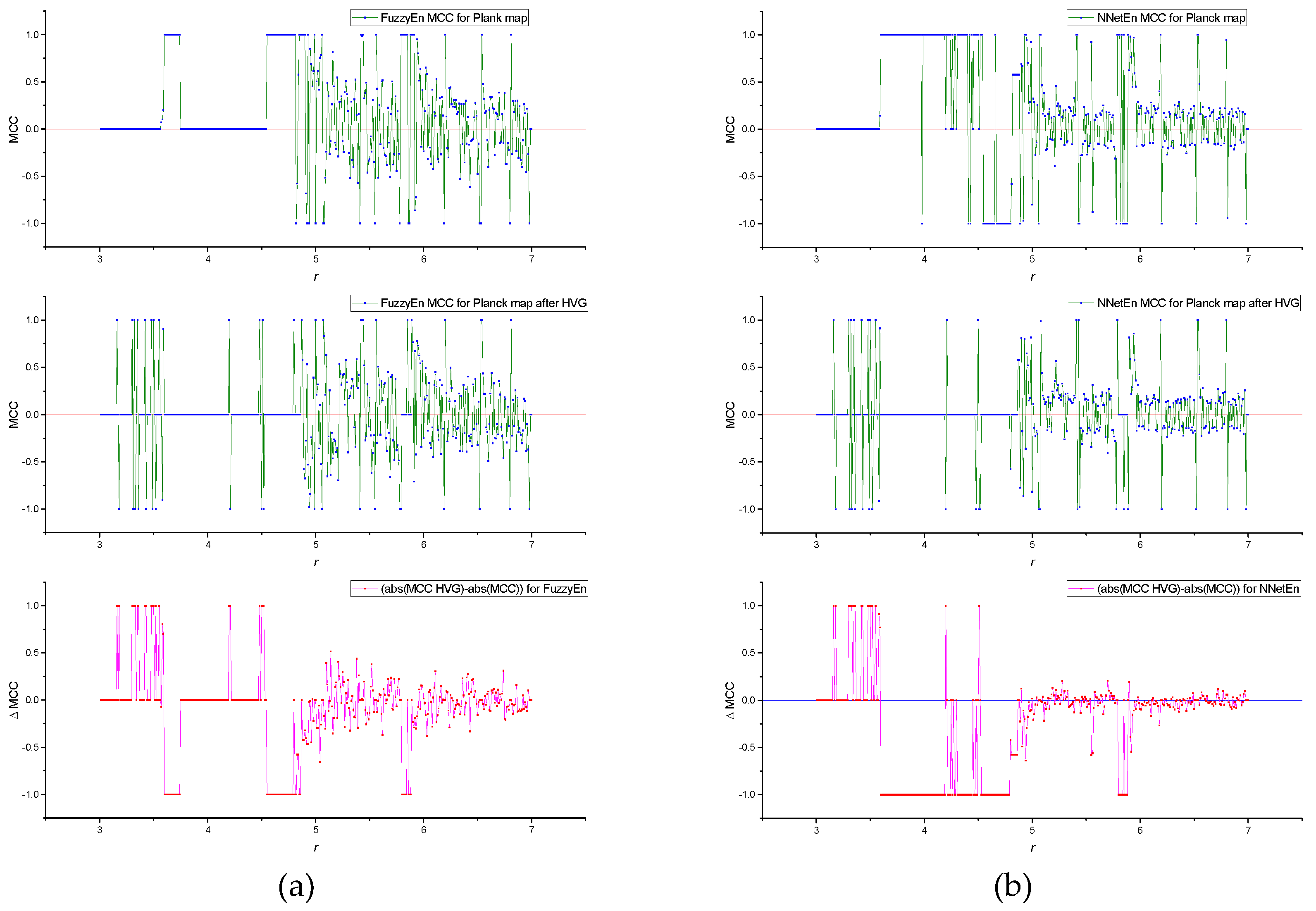
Figure A3a (Appendix A) shows an example of a bifurcation diagram for a Planck map in the control parameter range 3 ≤ r ≤ 7, with a sampling step dr = 0.01. Figure A3b,c shows the FuzzyEn_AV(r) and NNetEn_AV(r) dependences before and after applying the HVG transformation. Figure 4 shows the MCC(r) dependences for FuzzyEn and NNetEn before and after HVG transformation, and their difference ΔMCC.
3.2. Results for TMBM map
The TMBM map is a multi-parametric and more complex than the mappings from section 3.1. Figure 8a shows an example of a bifurcation diagram for a TMBM map in the control parameter range -1.7 ≤ r ≤ -1.5, with a sampling step dr = 0.0005.
After applying of the HVG transformation, there is a notable increase in the entropy values of FuzzyEn_AV, as depicted in Figure 8b. Additionally, Figure 8c illustrates a consistent decrease in NNetEn_AV across a wide range of r following the utilization of HVF. Figure 9 shows the dependencies of MCC(r) and the discernible differences, denoted as ΔMCC, before and after the HVG transformation for both FuzzyEn (refer to Figure 9a) and NNetEn (refer to Figure 9b).
Figure 10 shows that there are local areas of the time series dynamics in which the classification efficiency NNetEn is higher than FuzzyEn (ΔMCC > 0), but most of the graph has ΔMCC < 0.
4. Discussion and Conclusions
In this work, we have proposed a method for assessing the effectiveness of entropy features using chaotic mappings, that enables to explore the efficiency of entropy-based classification of time series.
From Table 1, we have seen that the FuzzyEn has a better GEFMCC performance without the use of HVG transformation. At the same time, there are local areas of the time series dynamics in which the classification efficiency of NNetEn is higher than using FuzzyEn (Figure 7 and Figure 10). Nevertheless, despite of reducing the amount of signal information after HVG transformations, we see that there are local areas of the time series dynamics in which the classification efficiency increases when an HVG transformation is applied to the time series (Figure 6, Figure 9, Figure A2 and Figure A4). As it has been already seen in other contexts, HVGT transformations preserve structural properties of the time series [15,18]
All chaotic mappings analyzed in this work, present a similar GEFMCC trend when applying HVGs, and when comparing FuzzyEn and NNetEn, which indicates the universality of this characteristic. It is necessary to consider the fact that the results are given for specific entropy settings; for other parameters, the results may differ radically, since the effectiveness of entropies very much depends on the entropy calculation parameters. For future research, differing types of entropies can be compared under different parameters on one of the maps, for example, on the sine map. In addition, it is interesting to identify the dependence of GEFMCC on the length of the time series. Also, further research should be conducted in exploring other dynamical systems, as it is the case of fractional dynamical systems based on the logistic and sine maps [37,38,39], where visibility graphs have been already considered [40].
The fact that FuzzyEn turned out to be more effective in classifying short (N = 300) time series than NNetEn confirmed the results of our work on the classification of EEG signals [1]. However, individual pairs of time series can be better classified by NnetEn; this was also confirmed in the EEG experiment, where one channel performed better when using NNetEn as a feature. In the same work on EEG signals, the idea was put forward that classification based on several features may be better and the use of FuzzyEn and NNetEn may lead to a synergistic effect.
Author Contributions
Conceptualization, J.A.C., A.V.; methodology, J.A.C., A.V., O.G.O., Y.I. and V.T.P.; software, A.V., O.G.O. and Y.I.; validation, J.A.C., A.V., O.G.O., Y.I. and V.T.P.; formal analysis, J.A.C., A.V., O.G.O., Y.I. and V.T.P.; investigation, J.A.C., A.V., O.G.O., Y.I. and V.T.P.; resources, J.A.C., A.V., O.G.O., Y.I. and V.T.P.; data curation, J.A.C., A.V., O.G.O., Y.I. and V.T.P.; writing—original draft preparation, J.A.C., A.V., O.G.O., Y.I. and V.T.P.; writing—review and editing, X.X.; visualization, J.A.C. and A.V.; supervision, J.A.C.; project administration, J.A.C.; funding acquisition, J.A.C. and A.V. All authors have read and agreed to the published version of the manuscript.
Funding
This research was supported by the Russian Science Foundation (grant no. 22-11-00055, https://rscf.ru/en/project/22-11-00055/, accessed on 30 March 2023).
Data Availability Statement
The data used in this study can be shared with the parties, provided that the article is cited.
Conflicts of Interest
The authors declare no conflict of interest.
Appendix A
Figure A1.
Bifurcation diagrams for sin map (a); the dependence of entropy on the parameter r for NNetEn_AV (b) and FuzzyEn_AV before and after HVG transformation (c).
Figure A1.
Bifurcation diagrams for sin map (a); the dependence of entropy on the parameter r for NNetEn_AV (b) and FuzzyEn_AV before and after HVG transformation (c).
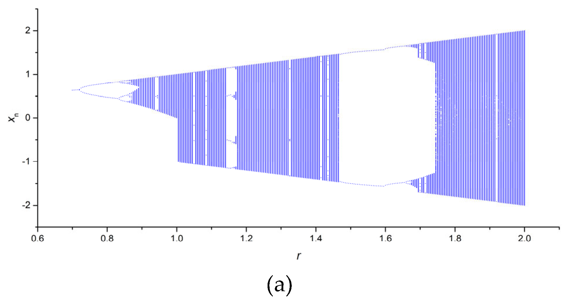
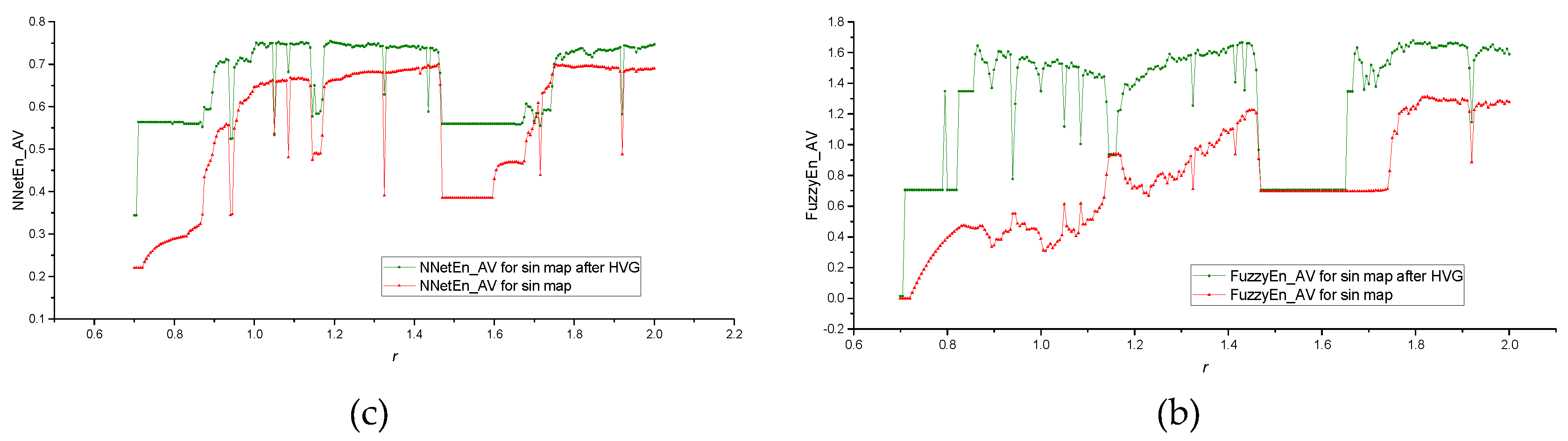
Figure A2.
MCC(r) dependences for FuzzyEn before and after HVG transformation, as well as their difference ΔMCC (a) MCC(r) dependences for NNetEn before and after HVG transformation, as well as their difference ΔMCC (b). Calculations were made for sin map.
Figure A2.
MCC(r) dependences for FuzzyEn before and after HVG transformation, as well as their difference ΔMCC (a) MCC(r) dependences for NNetEn before and after HVG transformation, as well as their difference ΔMCC (b). Calculations were made for sin map.
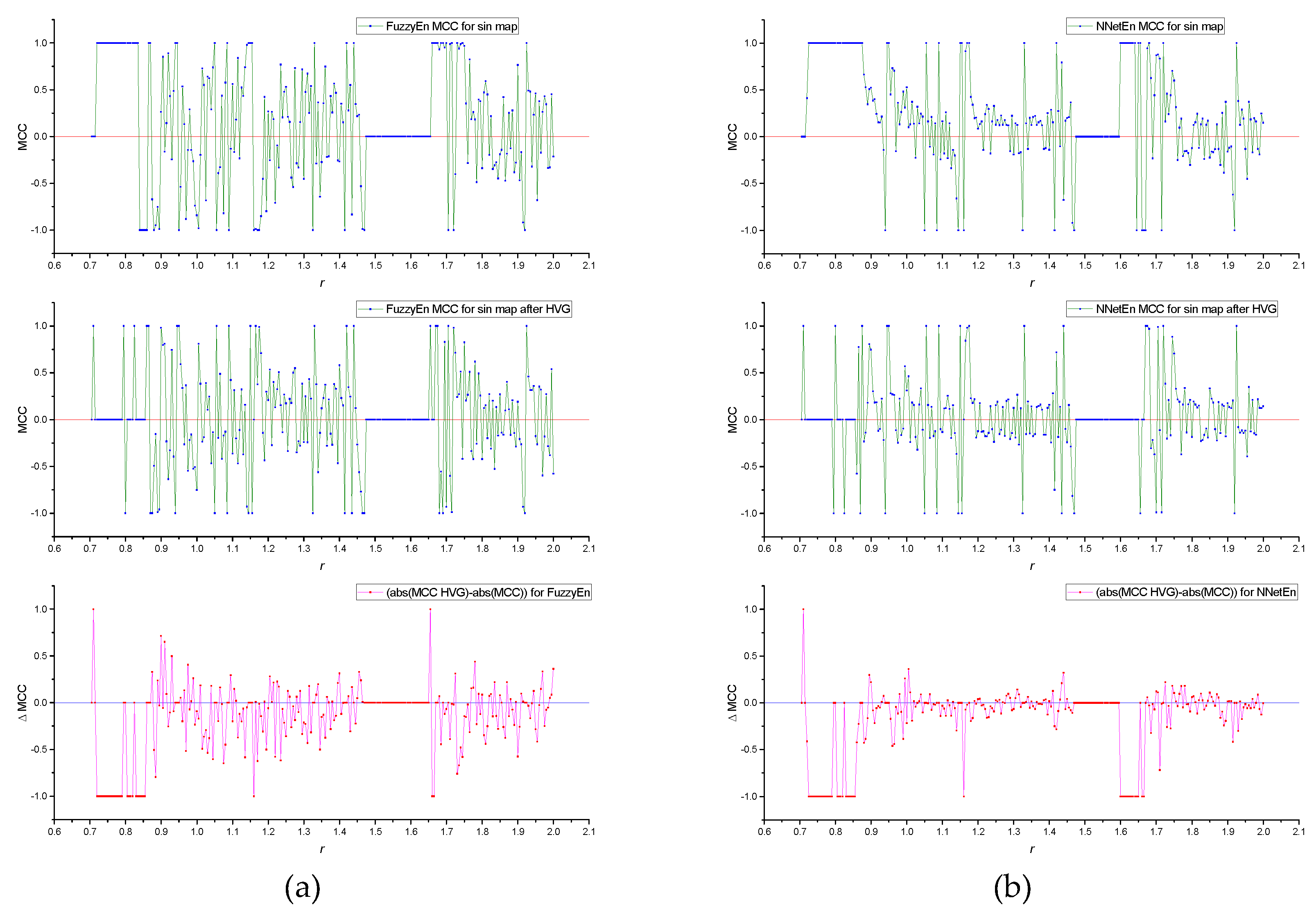
Figure A3.
Bifurcation diagrams for Planck map (a); the dependence of entropy on the parameter r for NNetEn_AV (b) and FuzzyEn_AV before and after HVG transformation (c).
Figure A3.
Bifurcation diagrams for Planck map (a); the dependence of entropy on the parameter r for NNetEn_AV (b) and FuzzyEn_AV before and after HVG transformation (c).
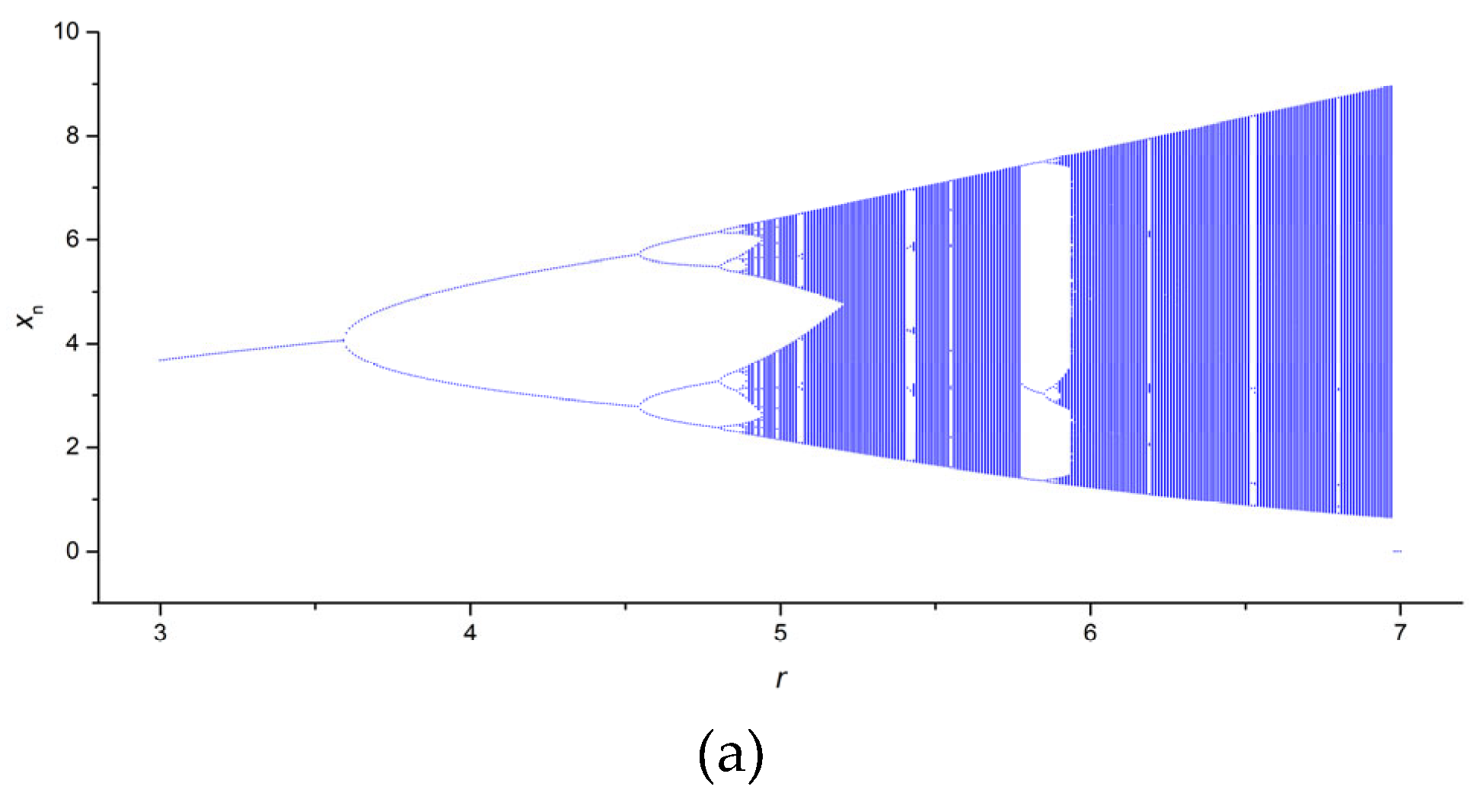
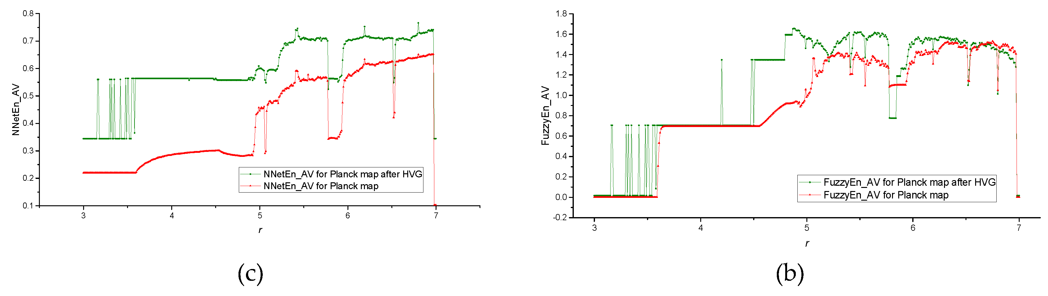
Figure A4.
MCC(r) dependences for FuzzyEn before and after HVG transformation, as well as their difference ΔMCC (a) MCC(r) dependences for NNetEn before and after HVG transformation, as well as their difference ΔMCC (b). Calculations were made for Planck map.
Figure A4.
MCC(r) dependences for FuzzyEn before and after HVG transformation, as well as their difference ΔMCC (a) MCC(r) dependences for NNetEn before and after HVG transformation, as well as their difference ΔMCC (b). Calculations were made for Planck map.
References
- Velichko, A.; Belyaev, M.; Izotov, Y.; Murugappan, M.; Heidari, H. Neural Network Entropy (NNetEn): Entropy-Based EEG Signal and Chaotic Time Series Classification, Python Package for NNetEn Calculation. Algorithms 2023, 16, 255. [Google Scholar] [CrossRef]
- Aoki, Y.; Takahashi, R.; Suzuki, Y.; Pascual-Marqui, R.D.; Kito, Y.; Hikida, S.; Maruyama, K.; Hata, M.; Ishii, R.; Iwase, M.; et al. EEG Resting-State Networks in Alzheimer’s Disease Associated with Clinical Symptoms. Sci Rep 2023, 13, 3964. [Google Scholar] [CrossRef] [PubMed]
- Belyaev, M.; Murugappan, M.; Velichko, A.; Korzun, D. Entropy-Based Machine Learning Model for Fast Diagnosis and Monitoring of Parkinson’s Disease. Sensors 2023, 23. [Google Scholar] [CrossRef]
- Yuvaraj, R.; Rajendra Acharya, U.; Hagiwara, Y. A Novel Parkinson’s Disease Diagnosis Index Using Higher-Order Spectra Features in EEG Signals. Neural Comput Appl 2018, 30, 1225–1235. [Google Scholar] [CrossRef]
- Aljalal, M.; Aldosari, S.A.; Molinas, M.; AlSharabi, K.; Alturki, F.A. Detection of Parkinson’s Disease from EEG Signals Using Discrete Wavelet Transform, Different Entropy Measures, and Machine Learning Techniques. Sci Rep 2022, 12, 22547. [Google Scholar] [CrossRef] [PubMed]
- Han, C.-X.; Wang, J.; Yi, G.-S.; Che, Y.-Q. Investigation of EEG Abnormalities in the Early Stage of Parkinson’s Disease. Cogn Neurodyn 2013, 7, 351–359. [Google Scholar] [CrossRef] [PubMed]
- Richman, J.S.; Moorman, J.R. Physiological Time-Series Analysis Using Approximate Entropy and Sample Entropy. American Journal of Physiology-Heart and Circulatory Physiology 2000, 278, H2039–H2049. [Google Scholar] [CrossRef]
- Chanwimalueang, T.; Mandic, D. Cosine Similarity Entropy: Self-Correlation-Based Complexity Analysis of Dynamical Systems. Entropy 2017, 19, 652. [Google Scholar] [CrossRef]
- Li, S.; Yang, M.; Li, C.; Cai, P. Analysis of Heart Rate Variability Based on Singular Value Decomposition Entropy. Journal of Shanghai University (English Edition) 2008, 12, 433–437. [Google Scholar] [CrossRef]
- Xie, H.-B.; Chen, W.-T.; He, W.-X.; Liu, H. Complexity Analysis of the Biomedical Signal Using Fuzzy Entropy Measurement. Appl Soft Comput 2011, 11, 2871–2879. [Google Scholar] [CrossRef]
- Bandt, C.; Pompe, B. Permutation Entropy: A Natural Complexity Measure for Time Series. Phys Rev Lett 2002, 88, 174102. [Google Scholar] [CrossRef] [PubMed]
- Velichko, A. Neural Network for Low-Memory IoT Devices and MNIST Image Recognition Using Kernels Based on Logistic Map. Electronics (Basel) 2020, 9, 1432. [Google Scholar] [CrossRef]
- Izotov, Y.A.; Velichko, A.A.; Ivshin, A.A.; Novitskiy, R.E. Recognition of Handwritten MNIST Digits on Low-Memory 2 Kb RAM Arduino Board Using LogNNet Reservoir Neural Network. IOP Conf Ser Mater Sci Eng 2021, 1155, 12056. [Google Scholar] [CrossRef]
- Lecun, Y.; Bottou, L.; Bengio, Y.; Haffner, P. Gradient-Based Learning Applied to Document Recognition. Proceedings of the IEEE 1998, 86, 2278–2324. [Google Scholar] [CrossRef]
- Lacasa, L.; Luque, B.; Ballesteros, F.; Luque, J.; Nuño, J.C. From Time Series to Complex Networks: The Visibility Graph. Proc Natl Acad Sci U S A 2008, 105, 4972–4975. [Google Scholar] [CrossRef]
- Lacasa, L.; Toral, R. Description of Stochastic and Chaotic Series Using Visibility Graphs. Phys Rev E Stat Nonlin Soft Matter Phys 2010, 82. [Google Scholar] [CrossRef] [PubMed]
- Luque, B.; Lacasa, L.; Ballesteros, F.J.; Robledo, A. Feigenbaum Graphs: A Complex Network Perspective of Chaos. PLoS One 2011, 6. [Google Scholar] [CrossRef] [PubMed]
- Flanagan, R.; Lacasa, L.; Nicosia, V. On the Spectral Properties of Feigenbaum Graphs. J Phys A Math Theor 2020, 53. [Google Scholar] [CrossRef]
- Luque, B.; Lacasa, L.; Ballesteros, F.; Luque, J. Horizontal Visibility Graphs: Exact Results for Random Time Series. Phys Rev E Stat Nonlin Soft Matter Phys 2009, 80. [Google Scholar] [CrossRef]
- Requena, B.; Cassani, G.; Tagliabue, J.; Greco, C.; Lacasa, L. Shopper Intent Prediction from Clickstream E-Commerce Data with Minimal Browsing Information. Sci Rep 2020, 10. [Google Scholar] [CrossRef]
- Iglesias Perez, S.; Criado, R. Increasing the Effectiveness of Network Intrusion Detection Systems (NIDSs) by Using Multiplex Networks and Visibility Graphs. Mathematics 2023, 11. [Google Scholar] [CrossRef]
- Akgüller, Ö.; Balcı, M.A.; Batrancea, L.M.; Gaban, L. Path-Based Visibility Graph Kernel and Application for the Borsa Istanbul Stock Network. Mathematics 2023, 11. [Google Scholar] [CrossRef]
- Li, S.; Shang, P. Analysis of Nonlinear Time Series Using Discrete Generalized Past Entropy Based on Amplitude Difference Distribution of Horizontal Visibility Graph. Chaos Solitons Fractals 2021, 144, 110687. [Google Scholar] [CrossRef]
- Hu, X.; Niu, M. Degree Distributions and Motif Profiles of Thue–Morse Complex Network. Chaos Solitons Fractals 2023, 176. [Google Scholar] [CrossRef]
- Gao, M.; Ge, R. Mapping Time Series into Signed Networks via Horizontal Visibility Graph. Physica A: Statistical Mechanics and its Applications 2024, 633. [Google Scholar] [CrossRef]
- Li, S.; Shang, P. A New Complexity Measure: Modified Discrete Generalized Past Entropy Based on Grain Exponent. Chaos Solitons Fractals 2022, 157. [Google Scholar] [CrossRef]
- May, R.M. Simple Mathematical Models with Very Complicated Dynamics. Nature 1976, 261, 459–467. [Google Scholar] [CrossRef]
- Sedik, A.; El-Latif, A.A.A.; Wani, M.A.; El-Samie, F.E.A.; Bauomy, N.A.; Hashad, F.G. Efficient Multi-Biometric Secure-Storage Scheme Based on Deep Learning and Crypto-Mapping Techniques. Mathematics 2023, 11. [Google Scholar] [CrossRef]
- Velichko, A.; Heidari, H. A Method for Estimating the Entropy of Time Series Using Artificial Neural Networks. Entropy 2021, 23. [Google Scholar] [CrossRef]
- Velichko, A.; Heidari, H. A Method for Estimating the Entropy of Time Series Using Artificial Neural Networks. Entropy 2021, 23. [Google Scholar] [CrossRef]
- Pham, V.-T.; Velichko, A.; Huynh, V. Van; Radogna, A.V.; Grassi, G.; Boulaaras, S.M.; Momani, S. Analysis of Memristive Maps with Asymmetry. Integration 2024, 94, 102110. [Google Scholar] [CrossRef]
- Lacasa, L.; Luque, B.; Ballesteros, F.; Luque, J.; Nuño, J.C. From Time Series to Complex Networks: The Visibility Graph. Proc Natl Acad Sci U S A 2008, 105, 4972–4975. [Google Scholar] [CrossRef] [PubMed]
- Carlos Bergillos Varela Ts2vg. Available online: https://pypi.org/project/ts2vg/.
- Chicco, D.; Warrens, M.J.; Jurman, G. The Matthews Correlation Coefficient (MCC) Is More Informative Than Cohen’s Kappa and Brier Score in Binary Classification Assessment. IEEE Access 2021, 9, 78368–78381. [Google Scholar] [CrossRef]
- Chen, W.; Wang, Z.; Xie, H.; Yu, W. Characterization of Surface EMG Signal Based on Fuzzy Entropy. IEEE Transactions on Neural Systems and Rehabilitation Engineering 2007, 15, 266–272. [Google Scholar] [CrossRef]
- Heidari, H.; Velichko, A.; Murugappan, M.; Chowdhury, M.E.H. Novel Techniques for Improving NNetEn Entropy Calculation for Short and Noisy Time Series. Nonlinear Dyn 2023. [Google Scholar] [CrossRef]
- Wu, G.-C.; Baleanu, D. Discrete Fractional Logistic Map and Its Chaos. Nonlinear Dyn 2014, 75, 283–287. [Google Scholar] [CrossRef]
- Wu, G.-C.; Niyazi Cankaya, M.; Banerjee, S. Fractional Q-Deformed Chaotic Maps: A Weight Function Approach. Chaos 2020, 30. [Google Scholar] [CrossRef] [PubMed]
- Wu, G.-C.; Baleanu, D.; Zeng, S.-D. Discrete Chaos in Fractional Sine and Standard Maps. Physics Letters, Section A: General, Atomic and Solid State Physics 2014, 378, 484–487. [Google Scholar] [CrossRef]
- Conejero, J.A.; Lizama, C.; Mira-Iglesias, A.; Rodero, C. Visibility Graphs of Fractional Wu–Baleanu Time Series. Journal of Difference Equations and Applications 2019, 25, 1321–1331. [Google Scholar] [CrossRef]
Figure 1.
Illustrative example of the NVG representation for a time series (left) and the HVG representation for the same time series (right).
Figure 1.
Illustrative example of the NVG representation for a time series (left) and the HVG representation for the same time series (right).
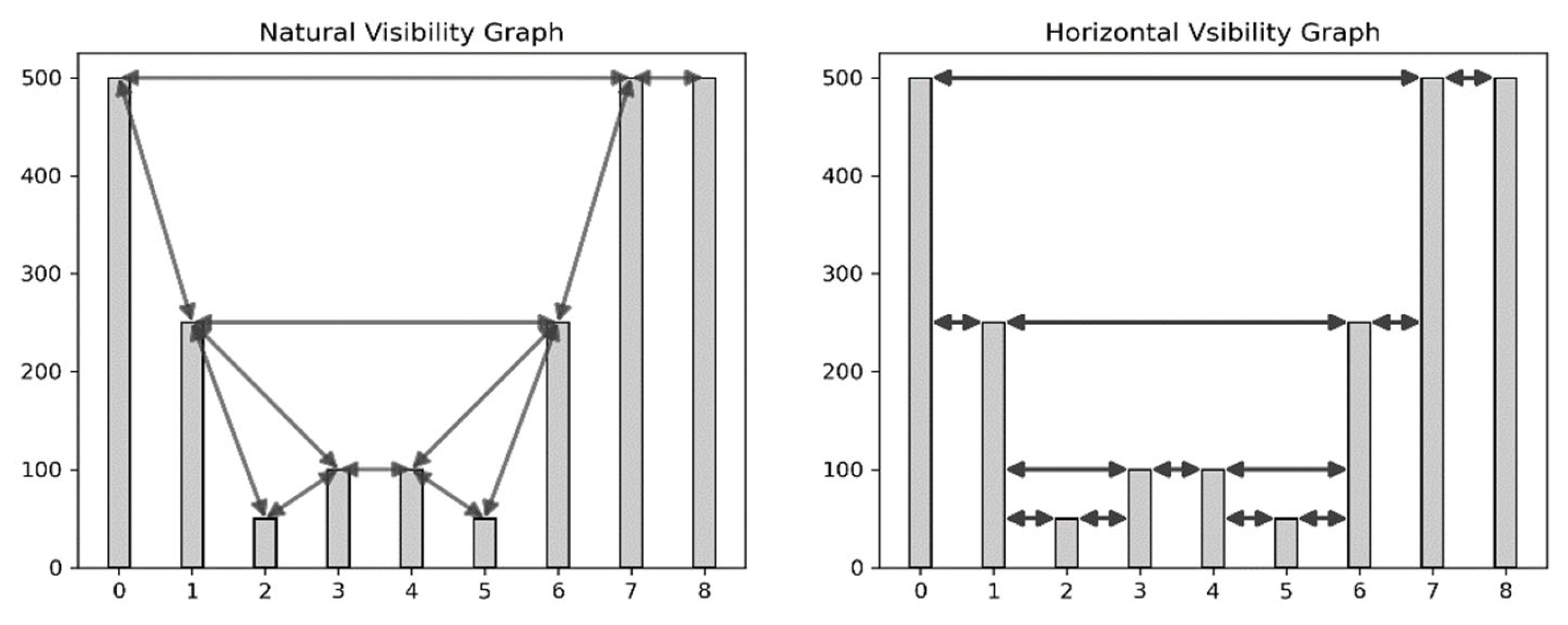
Figure 2.
Section of the buffering diagram of the logistic map, on which two adjacent sets of series are highlighted corresponding to rj-1 = 3.634 and rj = 3.636 (a), series (x1, …, x300) for rj-1 = 3.634 (b), series (x1, …, x300) for rj = 3.636 (c), FuzzyEn values for 100 time series for two classes (MCC = 1) (d).
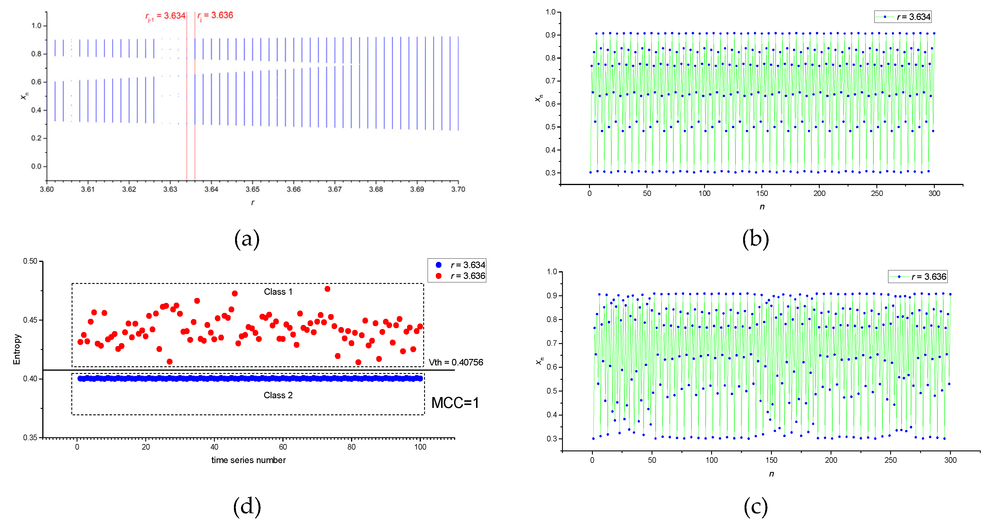
Figure 3.
Distribution of FuzzyEn in Classes 1 and 2 with rj-1 = 3.688 and rj = 3.69 (MCC~0.45).
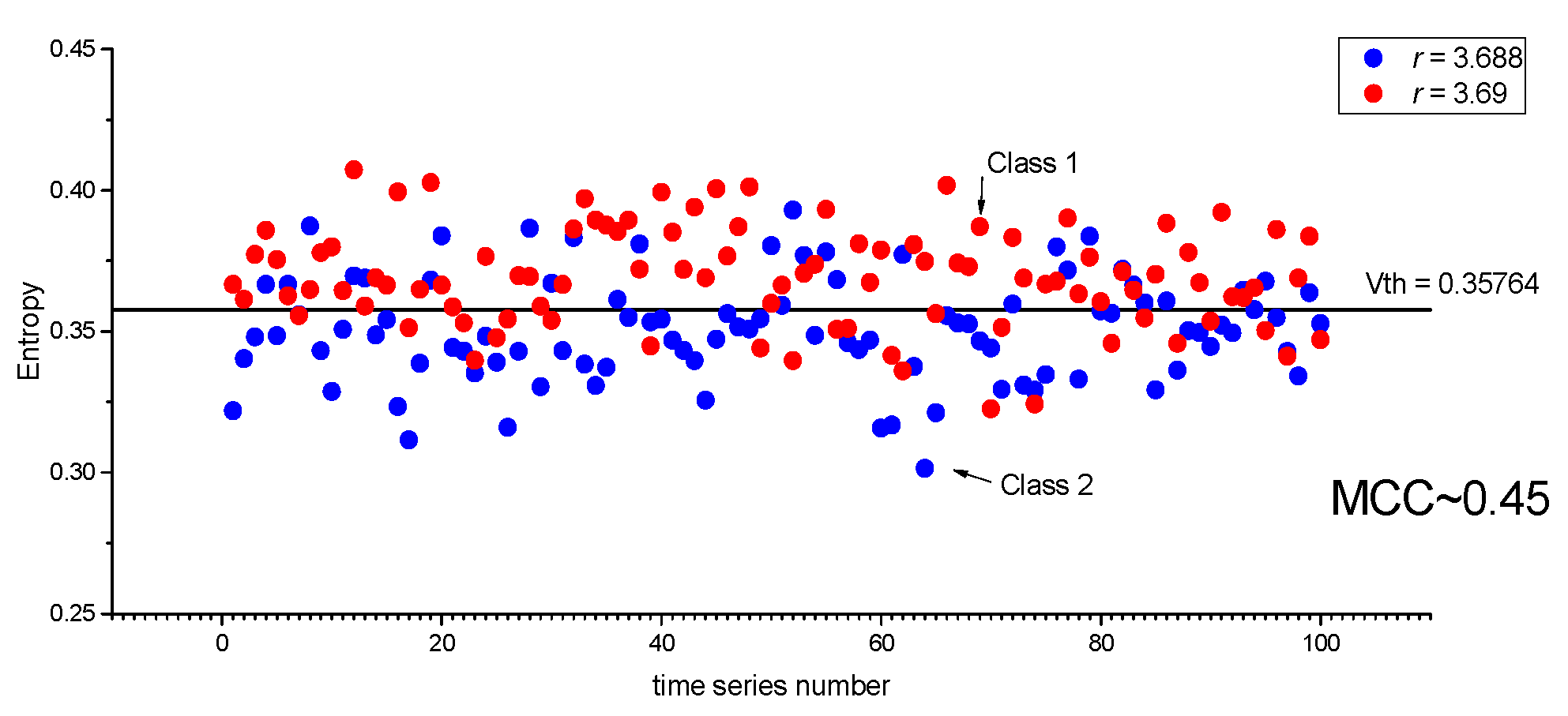
Figure 4.
Figure 4. Main steps of NNetEn calculation [1].
Figure 4.
Figure 4. Main steps of NNetEn calculation [1].
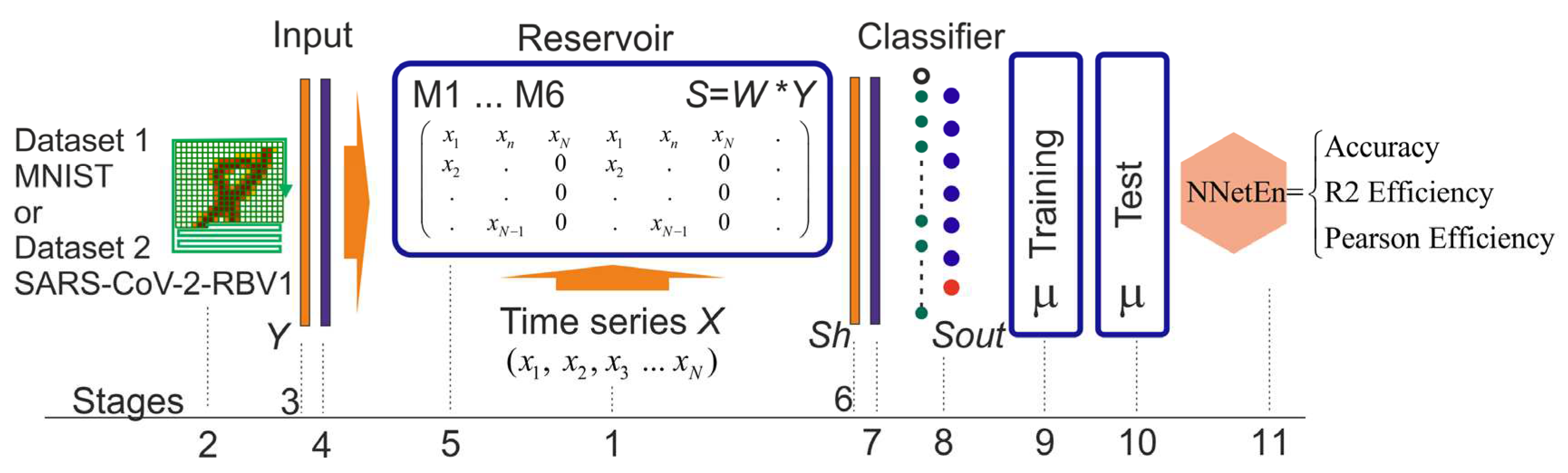
Figure 5.
Bifurcation diagrams for logistic map (a); the dependence of entropy on the parameter r for NNetEn_AV (b) and FuzzyEn_AV before and after HVG transformation (c).
Figure 5.
Bifurcation diagrams for logistic map (a); the dependence of entropy on the parameter r for NNetEn_AV (b) and FuzzyEn_AV before and after HVG transformation (c).
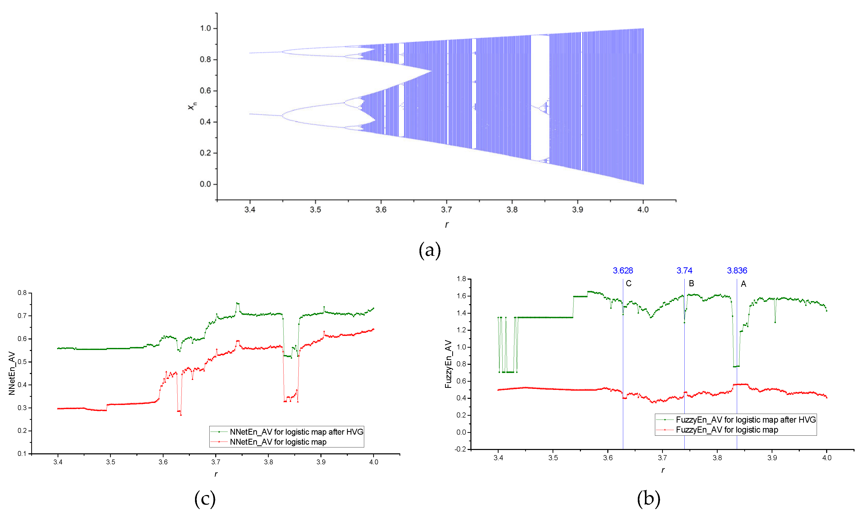
Figure 6.
MCC(r) dependences for FuzzyEn before and after HVG transformation, as well as their difference ΔMCC (a) MCC(r) dependences for NNetEn before and after HVG transformation, as well as their difference ΔMCC (b). Calculations were made for logistic map.
Figure 6.
MCC(r) dependences for FuzzyEn before and after HVG transformation, as well as their difference ΔMCC (a) MCC(r) dependences for NNetEn before and after HVG transformation, as well as their difference ΔMCC (b). Calculations were made for logistic map.
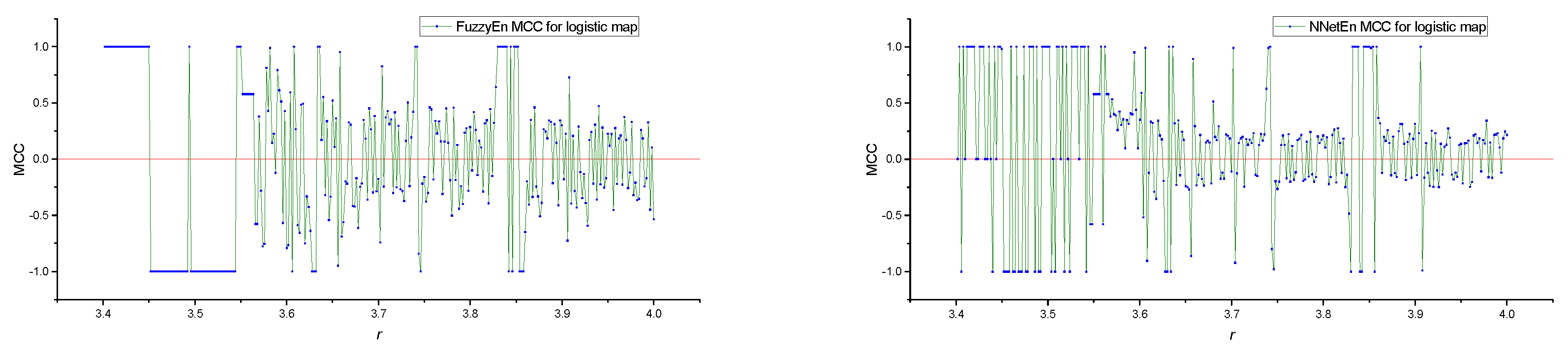
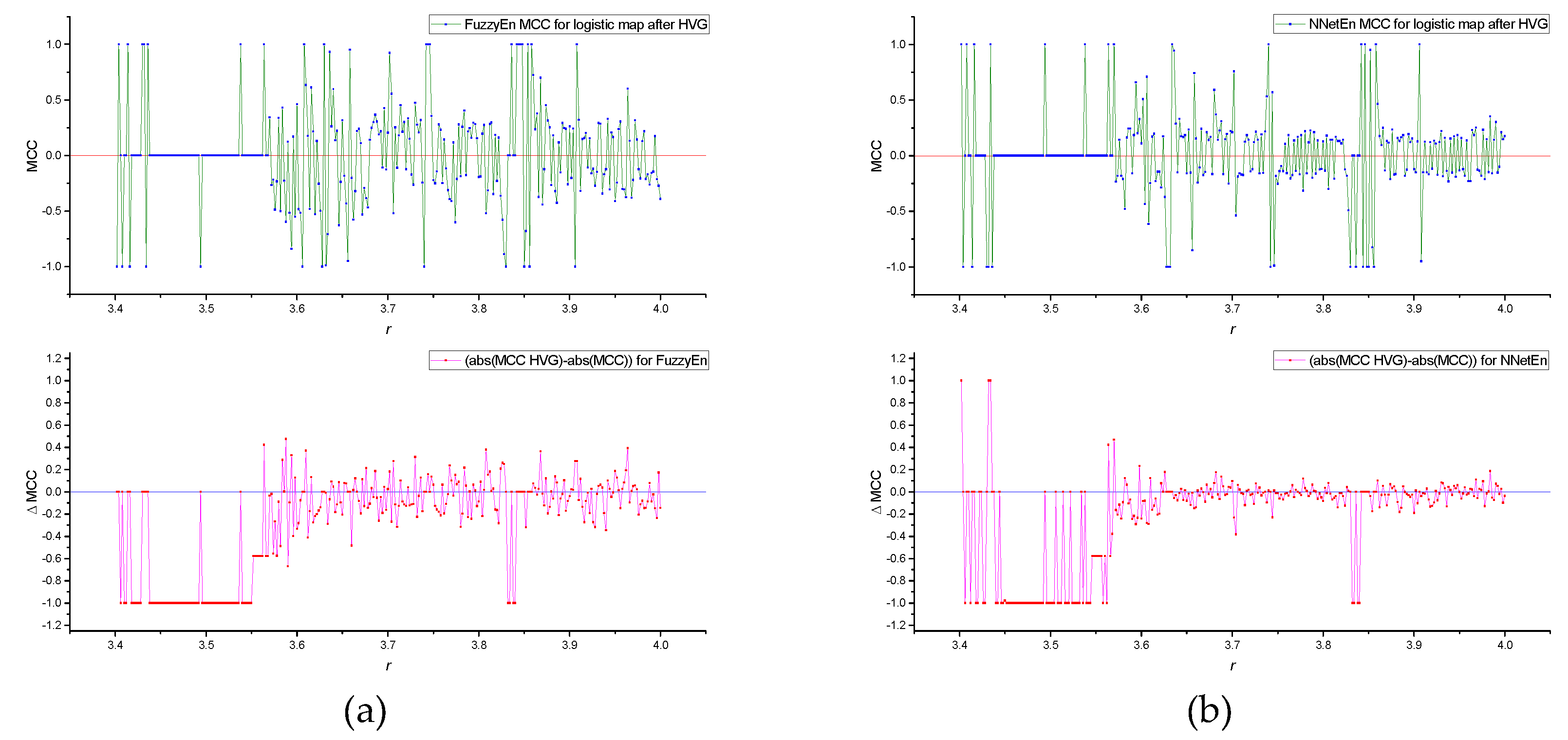
Figure 7.
ΔMCC(r) dependences for FuzzyEn and NeNetEn. Calculations were made for logistic map.
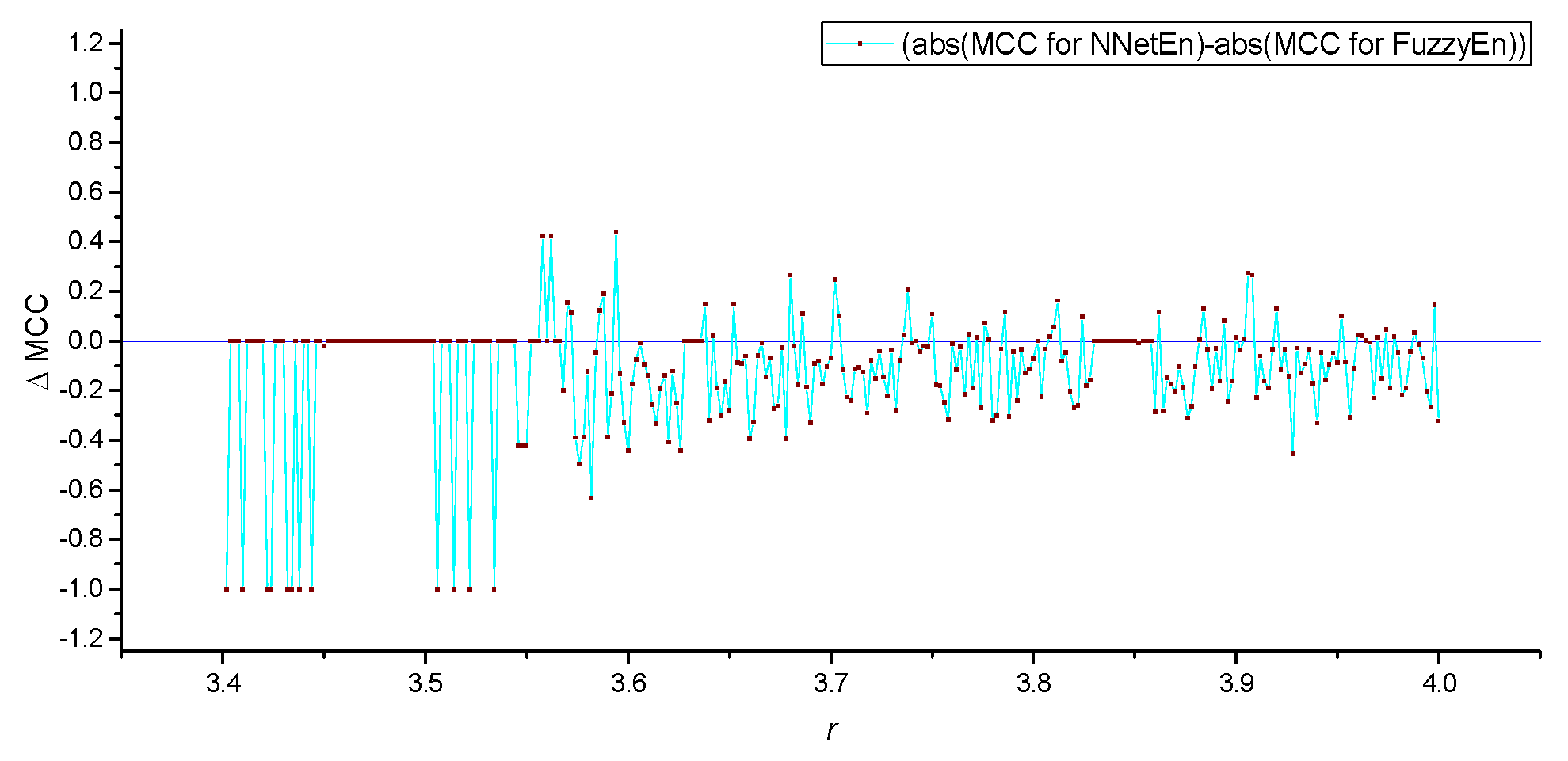
Figure 8.
Figure 8. Bifurcation diagrams for TMBM map (a); the dependence of entropy on the parameter r for NNetEn_AV (b) and FuzzyEn_AV before and after HVG transformation (c).
Figure 8.
Figure 8. Bifurcation diagrams for TMBM map (a); the dependence of entropy on the parameter r for NNetEn_AV (b) and FuzzyEn_AV before and after HVG transformation (c).
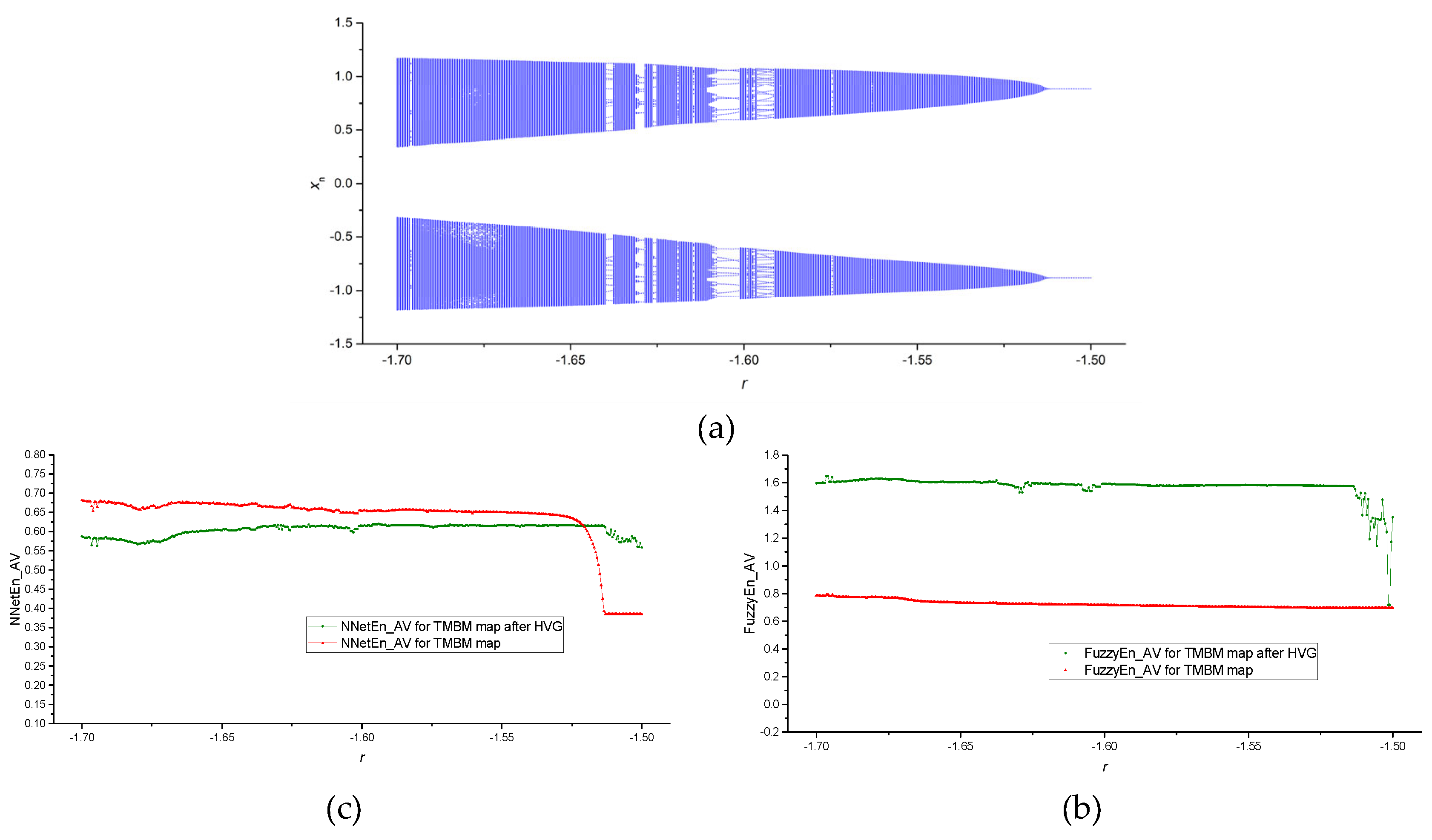
Figure 9.
MCC(r) dependences for FuzzyEn before and after HVG transformation, as well as their difference ΔMCC (a) MCC(r) dependences for NNetEn before and after HVG transformation, as well as their difference ΔMCC (b). Calculations were made for TMBM map.
Figure 9.
MCC(r) dependences for FuzzyEn before and after HVG transformation, as well as their difference ΔMCC (a) MCC(r) dependences for NNetEn before and after HVG transformation, as well as their difference ΔMCC (b). Calculations were made for TMBM map.
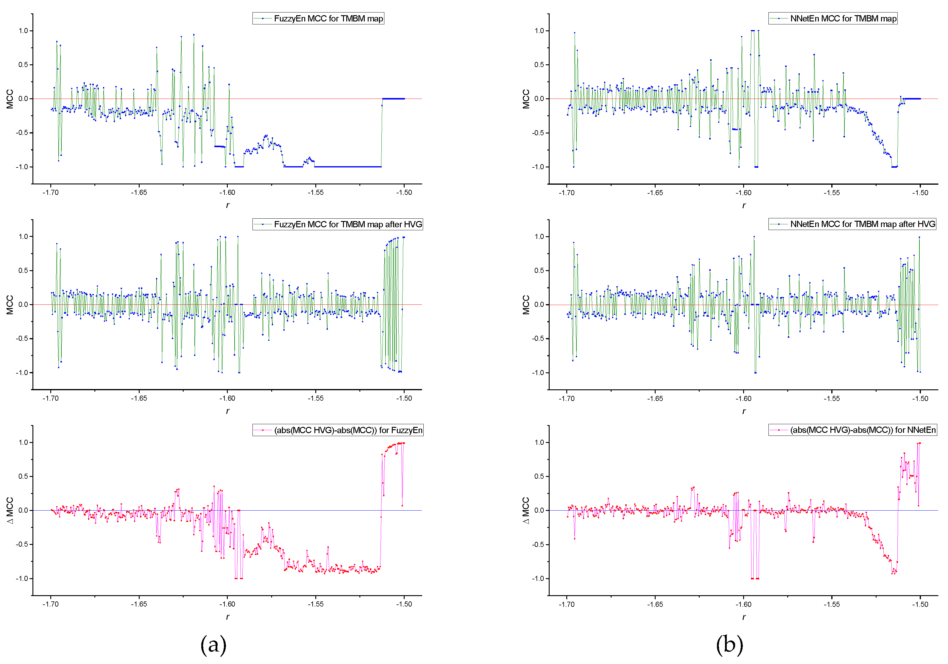
Figure 10.
ΔMCC(r) dependences for FuzzyEn and NeNetEn. Calculations were made for TMBM map.
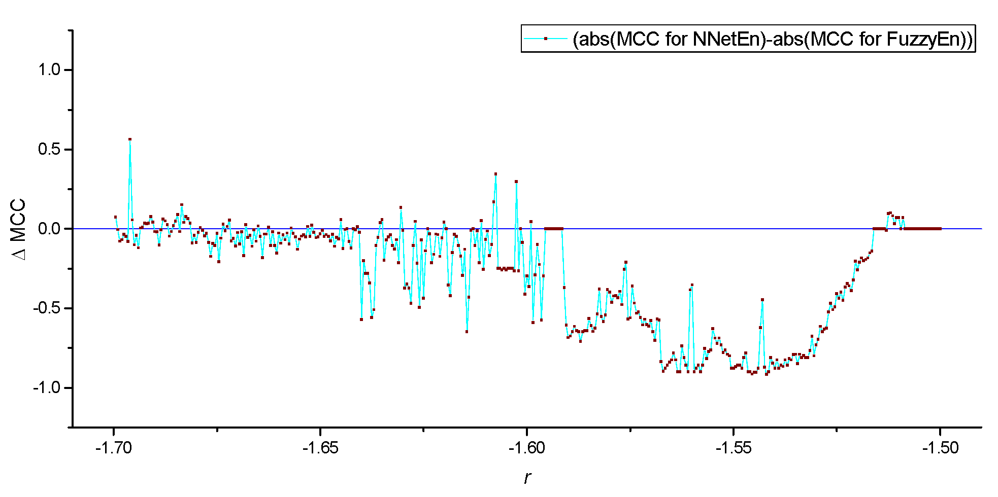

Table 1.
Comparison of GEFMCC value for different chaotic mappings and entropies, before and after HVG.
Table 1.
Comparison of GEFMCC value for different chaotic mappings and entropies, before and after HVG.
| GEFMCC | ||||
| Logistic map | Sine map | Planck map | TMBM map | |
| FuzzyEn no HVG | 0.578 | 0.524 | 0.359 | 0.544 |
| FuzzyEn after HVG | 0.310 | 0.366 | 0.267 | 0.256 |
| NNetEn no HVG | 0.463 | 0.436 | 0.482 | 0.255 |
| NNetEn after HVG | 0.245 | 0.266 | 0.208 | 0.216 |
Disclaimer/Publisher’s Note: The statements, opinions and data contained in all publications are solely those of the individual author(s) and contributor(s) and not of MDPI and/or the editor(s). MDPI and/or the editor(s) disclaim responsibility for any injury to people or property resulting from any ideas, methods, instructions or products referred to in the content. |
© 2023 by the authors. Licensee MDPI, Basel, Switzerland. This article is an open access article distributed under the terms and conditions of the Creative Commons Attribution (CC BY) license (http://creativecommons.org/licenses/by/4.0/).
Copyright: This open access article is published under a Creative Commons CC BY 4.0 license, which permit the free download, distribution, and reuse, provided that the author and preprint are cited in any reuse.


