Submitted:
26 December 2023
Posted:
28 December 2023
You are already at the latest version
Abstract
The three-axis stabilization geostationary remote sensing satellite features high time resolution and plays a significant role in weather forecasting and environmental monitoring. With the future development of satellite technology, we propose a rapid geolocation algorithm for three-axis stabilization geostationary remote sensing satellites from the perspective of software algorithms. The method assesses conventional remote sensing data geolocation methods and the coordination group for meteorological satellites (CGMS, Coordination Group for Meteorological Satellites) nominal grid publishing format. First, the initial incident viewing vector of each detector on the sensor was constructed. Then, by reflecting the satellite platform's east-west and north-south mirrors, the outgoing vector of the payload coordinate system was obtained. This vector was converted to the satellite body coordinate system and, subsequently, to the satellite orbit coordinate system. The conversion of the earth-fixed coordinate system and the mirror rotation angle under ideal CGMS grid conditions were obtained, and the mirror rotation angle was converted to the corresponding CGMS nominal grid position to complete data positioning. The algorithm omits the complex process of calculating the intersection point between the viewing vector and the geodetic ellipsoid sphere from the earth-fixed coordinate system, resulting in an 83.3% improvement in computational efficiency without compromising positioning accuracy compared with conventional geolocation methods. This algorithm greatly improves the processing efficiency of geostationary meteorological satellite positioning, but its limitation is that the data processing results must be released in the CGMS nominal grid format.
Keywords:
Three-axis Stabilization
; Geostationary orbit
; Remote Sensing Satellite
; Nominal Grid
; Coordination Group for Meteorological Satellites
; Rapid Geolocation Algorithm
1. Introduction
Geostationary orbit has become a contested strategic resource, with major powers vying for control. Geostationary orbit remote sensing satellites possess the unique advantage of being able to "see far and stay high," making them optimal for continuous and dynamic observation of targets. This has led to an increasing number of geostationary orbit satellite applications being used worldwide. Some notable examples include the US GOES-R [1], Japan's "Himawari 8/9 [2]", China's "GF-4 [3]", "Fengyun-4A [4]", and "Fengyun-4B [5]". Furthermore, the third-generation imaging satellite MTG-I1 of the European Organization for the Exploitation of Meteorological Satellites (EUMETSAT) was successfully launched on December 13, 2022.
Georeferencing of geostationary orbit remote sensing images is the cornerstone of subsequent applications of remote sensing data. Georeferencing algorithms for satellite images can be classified into non-parametric and parametric methods [6]. Non-parametric methods can be applied to all types of geometric distortions but require multiple ground control points to establish a mapping relationship between remote sensing data and geographic coordinates. However, they are unsuitable for georeferencing automated operational geostationary satellite imagery, such as the Fengyun series, due to the time- and resource-intensive process of selecting high-precision ground control points. Moreover, it remains challenging to identify usable ground control points in cloudy conditions, which fails to meet the requirements of high timeliness and stability for meteorological satellite operations [7,8]. In contrast, parametric methods establish models based on the observation geometry, spatial position, and pointing of satellite sensors to calculate the georeferencing information of remote sensing data [9]. Ground control points are used to eliminate georeferencing errors caused by uncertainties in model param [10,11,12], and terrain information is utilized to remove georeferencing errors caused by surface topography. These errors depend on satellite altitude, terrain, and the distance between observation and nadir points [13]. This paper focuses on parametric methods for georeferencing, particularly those tailored for geostationary orbit meteorological satellite imagery.
Geostationary orbit remote sensing satellites have two primary modes of observation: full disk and regional. Full-disk observation is primarily utilized to support the tracking of large-scale weather systems, numerical weather prediction applications, and climate dataset construction. Regional observation is mainly conducted for weather systems on a scale of 1,000–2,000 km, specifically to monitor small to medium-scale convective systems and typhoons, providing weather analysis and warning services [14].
As shown in Table 1, the current full disk observation time efficiency is 5 min for the US GOES-R series, Japan's Himawari-8/9 satellites, 10 min for MTG-I1, and 15 min for Fengyun-4A and Fengyun-4B satellites [15,16]. In terms of medium-scale regional scan time, Himawari-8/9 requires 2.5 min for typhoon-scale regional observation, Fengyun-4A requires 3 min for typhoon-scale regional observation, and Fengyun-4B's rapid imaging instrument requires 1 min for a 2000×2000 km regional observation. In terms of spatial resolution, GEOS-R, Himawari-8/9, and Fengyun-4A are similar, while Fengyun-4B can achieve the highest resolution of 0.25 km. Remote sensing applications such as weather forecasting and environmental monitoring increasingly demand real-time processing of remote sensing data, even at a minute level. With the improvement of the spatial resolution of remote sensing satellites, the volume of acquired data increases significantly, requiring higher efficiency in data processing and georeferencing calculations. For example, the spatial resolution of Fengyun-4B's rapid imaging instrument is 250 m, which is twice the resolution of existing imagers. Efficient georeferencing algorithms can meet the requirements of regional observation but cannot satisfy the needs of full-disk observation with rapid imaging instruments. Therefore, to achieve efficient processing of geostationary orbit remote sensing satellite data, it is crucial to research more efficient georeferencing algorithms that have practical significance and economic value in addition to hardware improvements.
This paper centers on the param-based geolocation process commonly utilized for three-axis stabilized geostationary orbit remote sensing satellites. Based on our analysis of the standard data release format of geostationary orbit satellite products, we propose a rapid geolocation algorithm and confirm its feasibility through experiments.
2. Algorithm Principle
2.1. Conventional Geolocation Process Based on Intersection of Viewing Vectors
Three-axis stabilized geostationary orbit remote sensing satellites often adopt a dual scanner drive mode, where scanning mirrors are driven in an east-west direction for cross-track scanning and in a north-south direction for along-track stepping, enabling large-area coverage. Figure 1 presents the scanning mechanism and ideal optical path of the satellite payload.
The geolocation algorithm utilizes the scanning mirror angles from the sensor's Level 0 data to computationally determine the corresponding ground latitude and longitude. This conventional geolocation algorithm commences by modeling the instrument's observation geometry to acquire the initial viewing vectors for each pixel. Through a series of coordinate transformations, the image-plane coordinates are projected onto the Earth-fixed coordinate system. The algorithm then computes the intersection coordinates of the sensor's viewing vector with the ground, which are subsequently transformed into latitude and longitude. Finally, these coordinates are mapped onto the coordination group for meteorological satellites (CGMS) grid (a nominal grid with a specific projection defined by the coordination group for meteorological satellites), one of the international standards for meteorological remote sensing. The specific coordinate system transformations involved in this process are graphically depicted in Figure 2.
The initial viewing vector, denoted as , varies with the changes in the angles of the two scanning mirrors. Assuming the outgoing ray vector in the payload coordinate system is , the resulting viewing vector after two reflections from the scanning mirrors, denoted as , was expressed as:
Here, 𝐹1 and 𝐹2 are the reflection matrices for the north-south and east-west mirrors, respectively. These matrices are determined by the angles of rotation 𝛼 for the north-south mirror and 𝛽 for the east-west mirror. The specific derivation process can be found in references [17,18,19].
After the viewing vector exits the satellite body, it is transformed from the satellite body coordinate system to the Earth-fixed coordinate system based on the satellite attitude information, orbit information, and param such as nutation, precession, Greenwich sidereal time, and polar motion. For a given time , the geolocation process for the viewing vector in the payload coordinate system can be divided into the following eight steps:
1) calculating the viewing vector in the payload coordinate system based on the mirror angles and the optical path geometry ;
2) transforming the viewing vector from the payload coordinate system to the body coordinate system by using the installation matrix, obtaining ;
3) based on the orbit attitude, transforming the viewing vector from the body coordinate system to the orbit coordinate system, obtaining .The satellite body coordinate system was rotated in the order of and to obtain the orbit coordinate system.
4) based on the satellite's position and velocity, transforming the viewing vector from the orbit coordinate system to the Earth-centered inertial coordinate system.
The transformation from the orbit coordinate system to the Earth-centered inertial coordinate system is determined by the satellite's instantaneous inertial frame of reference, which considers the position and velocity. This transformation can be obtained by constructing the orbit coordinate system in the inertial frame of reference. The Earth-centered inertial coordinate system was with unit vectors as . The orbit coordinate system waswith unit vector For any given satellite position vector in the Earth-centered inertial coordinate system, the coordinates of the orbit coordinate system's axes were obtained using the following formula:
According to the definition of the orbit coordinate system, we derived:
The unit vector , which is orthogonal to both and the satellite's position vector , were determined by the following equation:
where is the velocity vector in the Earth-centered inertial coordinate system. Therefore, the unit vector was determined by the following equation:
By performing the calculations mentioned above, the transformation matrix from the orbit coordinate system to the Earth-centered inertial coordinate system was obtained as follows:
5) transforming the viewing vector from the Earth-centered inertial coordinate system to the Earth-fixed coordinate system based on time information.
This step mainly relies on information such as precession, nutation, Greenwich sidereal time, and polar motion to transform the viewing vector and satellite position vector from the Earth-centered inertial coordinate system to the Earth-fixed coordinate system. As a result, the viewing vector in the Earth-fixed coordinate system was obtained as follows:
Satellite position vector in the Earth-fixed coordinate system was calculated as:
Here, the subscript WGS represents the Earth-fixed coordinate system. denotes the precession correction matrix, represents the nutation correction matrix, signifies the Greenwich sidereal time rotation matrix, denotes the polar motion correction matrix, and represents the direction cosine matrix from the Earth-centered inertial coordinate system to the Earth-fixed coordinate system.
6) computing the position vector of the intersection point between the viewing vector and the WGS84 ellipsoid in the Earth-fixed coordinate system.
In the Earth-fixed coordinate system, the coordinates of the intersection point between the viewing vector and the surface of the Earth represented by the WGS-84 geodetic reference ellipsoid were calculated. The equation for the WGS-84 geodetic reference ellipsoid was represented as:
where represents the major axis and represents the minor axis. The intersection point between the viewing vector and the Earth's surface was calculated using formula (12) as follows:
represents the distance between the satellite and the intersection point:
7) converting the coordinates of the intersection point in the Earth-fixed coordinate system to the coordinates in the geodetic coordinate system.
Based on the coordinates of the intersection point in the Earth-fixed coordinate system, the geographic latitude and longitude of the intersection point were calculated using formula (13) as follows:
8) Based on the latitude and longitude of the intersection point, its row and column number (I,J) were calculated on the CGMS grid.
By employing the latitude and longitude coordinates, in conjunction with the north-south scan angle, east-west scan angle, satellite's geolocation, and the Earth model employed, it is possible to computationally determine the row and column number of the point on the nominal grid. For specific details regarding the calculation methodology, please refer to reference [16].
The computation time and proportion of each step for the conventional geolocation algorithm were computed using simulated data. The results are presented in Table 2.
2.2. Rapid Geolocation Algorithm for CGMS Nominal Grid
The nominal data format is the most commonly employed format for applying and disseminating geostationary remote sensing data. For instance, China's FY-2 and FY-4 L1A level data, along with the United States' GOES-R satellite L1B level data, are all published in nominal data formats [14]. The nominal grid comprises fixed observation angles with equal intervals, ensuring that identical data points in all products correspond to the same location on Earth. This provides a basis for further applications of remote sensing imagery. Currently, most geostationary meteorological satellites employ image geolocation methods based on the nominal grid. This allows each pixel in the remote sensing image to be associated with a specific latitude and longitude on Earth. Therefore, there is no need to store latitude and longitude information within the image data itself, significantly reducing the requirements for data transmission and storage.
The geolocation algorithm has a strict correspondence between the initial ray vectors of the remote sensing sensor's pixels, latitude, longitude, and the CGMS nominal grid. The row-column numbers (I, J) of the nominal grid have a unique correspondence with the geographic latitude and longitude (B, L). Therefore, during data geolocation, it is possible to first calculate the row-column numbers (I, J) of the ray vectors on the nominal grid and then obtain the corresponding geographic latitude and longitude (B, L) through a quick query. The ultimate goal of geolocation is to compute the position of the ray on the CGMS nominal grid. By analyzing the transformation process of the ray vector in different coordinate systems, this paper proposes a rapid algorithm that eliminates the time-consuming process of computing latitude and longitude. Instead, it directly establishes the correspondence between the ray vectors of the remote sensing sensor's pixels in the satellite body coordinate system and the CGMS nominal grid's row-column numbers (I, J), thus achieving the final geolocation.
After converting the viewing vector from the Earth-centered inertial coordinate system to the Earth-fixed coordinate system, errors caused by attitude, orbit, precession, nutation, Greenwich sidereal time, and polar motion are eliminated. It can be considered an idealized viewing vector in the satellite body coordinate system.
At this point, the viewing vector in the Earth-fixed coordinate system can be directly transformed into the equivalent ideal state in the satellite body coordinate system. The representation of this viewing vector was given as:
where represents the transformation matrix from the Earth-fixed coordinate system to the satellite body coordinate system. The specific method for numerical conversion between the geostationary sensor imaging grid and the CGMS grid can be found in reference [16,17].
Based on the viewing vector in the satellite body coordinate system, the relationship between the corresponding CGMS mirror angles was established as follows:
The values were calculated as follows:
Subsequently, the corresponding for were calculated as follows:
where represents the size of the nominal grid, and is the angular size of a pixel in this band.
Through the aforementioned refinements, the computationally burdensome process of finding the intersection point between the viewing vector and the Earth's ellipsoid was obviated. Instead, a direct mapping relationship was established between the original initial vector and the nominal grid. In the geolocation process, after transforming the ray vector into the Earth-fixed coordinate system, the positioning result was obtained directly through the conversion relationship between the ray vectors in the sensor imaging grid and the CGMS grid, without the need for iterative calculations to solve for the intersection point between the ray and the Earth's ellipsoidal surface. The flowchart of the improved rapid geolocation algorithm can be found in Figure 3.
Figure 3 illustrates that in the rapid algorithm flow, the calculations prior to the Earth-fixed coordinate system are consistent with the conventional algorithm flow. In the Earth-fixed coordinate system, the viewing vector no longer intersects with the geodetic ellipsoid. Instead, the viewing vector in the Earth-fixed coordinate system is transformed into the ideal state in the satellite body coordinate system. This is equivalent to the viewing vector of the actual satellite's downlink data being transformed into the idealized viewing vector (i.e., the corrected viewing vector after considering various error factors) through positioning and compensation calculations. Then, the mirror angles corresponding to the idealized viewing vector are calculated. By using the relationship between the angles and the initial position, along with the angle step size, the corresponding row-column numbers can be computed.
3. Experiment and Analysis
To validate the feasibility of the proposed algorithm, programming experiments were conducted using C++. The efficiency and accuracy of the geolocation calculations were compared. The computer environment used was an 11th Gen Intel(R) Core(TM) i7-1165G7@2.80GHz processor with 16 GB of memory, running on a 64-bit Windows 10 operating system.
3.1. Efficiency Comparison
To compare the computational efficiency of each step, we took a sample of geospatial observation data with a spatial resolution of 250 m. We simulated 10 million uniformly distributed nominal grid points within the full disk range, corresponding to 10 million sets of mirror angles. Employing both algorithms, we performed geolocation calculations and recorded the time consumption for each step, as shown in Table 2.
The percentage increase in computational efficiency () can be calculated as follows:
We observed that the rapid geolocation algorithm eliminated the time-consuming Earth-fixed to Geodetic coordinate transformation process compared to the conventional geolocation algorithm. This results in an improvement in computational efficiency of 83.3%.
3.2. Accuracy Comparison of Algorithms
To verify the accuracy of the two algorithms, representative regions were selected for statistical analysis of the geolocation results. These regions include the satellite subpoint area, the region towards the western edge of the Earth, and the region towards the northern edge of the Earth. The geolocation results in these three regions are presented in magnified display maps in Figure 4, Figure 5 and Figure 6. The line segment in the middle represents the east-west and north-south directions of the satellite coverage. The dots represent the IJ positions of the rapid algorithm on the CGMS nominal grid, while the circles represent the IJ positions of the conventional algorithm on the CGMS nominal grid. The difference between the positions of the dots and circles represents the difference in calculation results for the viewing vector corresponding to the same set of mirror angles. In the satellite subpoint area, the dots and circles coincide very well, but there is a slight difference as we move towards the edges of the Earth. To analyze the magnitude of this difference, the differences between the positions of the dots and circles in the three regions were statistically analyzed, as shown in Table 3. It can be observed that the mean difference in the geolocation results between the two algorithms is in the order of 10-5 pixels in the satellite subpoint area and in the order of 10-2 pixels in the regions towards the western and northern edges of the Earth. Therefore, it can be concluded that the computational accuracy of the two geolocation algorithms is comparable.
Table 3 lists the statistical values of the geolocation differences in the three test regions.
In summary, through simulation experiments, the proposed rapid geolocation algorithm for CGMS has been verified to achieve an 83.3% improvement in computational efficiency compared to that observed in the conventional geolocation algorithm without any loss in computational accuracy.
4. Conclusion
With the development of geospatial observation technology in geostationary orbit remote sensing, enhancing the timeliness of remote sensing data processing is crucial for improving practical and economic value. In this paper, by analyzing the conventional geolocation methods for geostationary orbit remote sensing satellite data and the data format of CGMS, we propose a fast geolocation algorithm for three-axis stabilized geostationary scanning remote sensing satellite images, specifically designed for CGMS nominal grids. This algorithm eliminates the computationally intensive process of calculating the intersection points between the viewing vectors and the Earth ellipsoid in the Earth-fixed coordinate system, thus improving the efficiency of geolocation calculations. Through experimental analysis with simulated data, the proposed rapid geolocation algorithm achieves improved timeliness in the geolocation processing of geostationary orbit remote sensing data without sacrificing accuracy when compared to conventional geolocation methods. This research provides a reference for efficient geolocation processing of geospatial observation data in geostationary orbit remote sensing.
Author Contributions
Conceptualization, He Li; Formal analysis, Congzhou Guo and Yuekun Sun ; Funding acquisition, He Li and Xiaochong Tong; Methodology, Chunping Qiu; Project administration, He Li; Supervision, Chunping Qiu; Validation, Jian Shang and Zhichao Wang ; Writing – original draft, He Li; Writing – review & editing, Xiaochong Tong. All authors have read and agreed to the published version of the manuscript.
Funding
This study was funded by Natural Science Foundation of Henan Province under Grant (Grant No. 212300410096 and 222300420592).
Conflicts of Interest
The authors declare no conflict of interest.
References
- Sullivan, P.; Krimchansky, A.; Walsh, T. An overview of the design and development of the geostationary operational environmental satellite R-series (GOES-R) space segment. EUMETSAT Meteorological Satellite Conference, NASA Goddard Space Flight Center, 2017, 20170009466.
- Bessho, K.; Date, K.; Hayashi, M.; Ikeda, A.; Yoshida, R. An introduction to Himawari-8/9—Japan’s new-generation geostationary meteorological satellites. J. Meteorol. Soc. Jpn 2016, 94, 151–183. [Google Scholar] [CrossRef]
- Wang, Dianzhong, and Hongyan He. "Observation capability and application prospect of GF-4 satellite." In 3rd International Symposium of Space Optical Instruments and Applications: Beijing, China -29th 2016, Springer International Publishing, 2017; pp. 393-401. 26 June.
- Yang, J.; Zhang, Z.; Wei, C.; Lu, F.; Guo, Q. Introducing the new generation of Chinese geostationary weather satellites–FengYun4 (FY-4). Bull. Am. Meteorol. Soc. 2016. [Google Scholar]
- Xian, D. FY-4B satellite. Satell. Appl. 2021. [Google Scholar] [CrossRef]
- Guan, M.; Wu, R. Geolocation approach for FY-3A MERSI remote sensing image. J. Appl. Meteorol. Sci. 2012, 23, 05–534. [Google Scholar]
- Roy, D.P.; Devereux, B.; Grainger, B.; White, S.J. Parametric geometric correction of airborne thematic mapper imagery. Int. J. Remote Sens. 1997, 18, 1865–1887. [Google Scholar] [CrossRef]
- Yang, L.; Yang, Z. The Automated Landmark Navigation of the Polar Meteorological Satellite. J. Appl. Meteorological Sci. 2009, 3, 329–336. [Google Scholar] [CrossRef]
- Wu, R.; Yang, Z.; Guan, M.; Li, X.X. Improved FY-3B/MERSI geolocation accuracy using installation matrix. Journal of Image and Graphics. 2012, 17, 10–1327. [Google Scholar]
- Rosborough, G.W.; Baldwin, D.G.; Emery, W.J. Precise AVHRR image navigation. IEEE Trans. Geosci. Remote Sens. 1994, 32, 644–657. [Google Scholar] [CrossRef]
- Moreno, J.F.; Melia, J. A method for accurate geometric correction of NOAA AVHRR HRPT data. IEEE Trans. Geosci. Remote Sens. 1993, 31, 204–226. [Google Scholar] [CrossRef]
- Cheng, K.; Tong, X.; Liu, S.; Yan, X.; Li, H. An on-orbit geometric calibration approach based on double tubes edge-binding Feng Yun-4A lightning mapping imager. J. Geom. Sci. Technol. 2021, 38, 8. [Google Scholar] [CrossRef]
- Lin, D.; Qin, Z.; Tong, X.; Li, H. Elevation correction method for earth observation of geostationary satellites. Inf. Sci. Journal of the Wuhan University 2017, 42, 6–851. [Google Scholar] [CrossRef]
- Zhang, X.; Feng, L.; Fangli, D.; Jianmin, X. Analysis on the observation model of foreign geostationary meteorological satellite. Adv. Meteorol. Sci. Technol.
- Wang, G.; Chen, G. Two-dimensional scanning infrared imaging technology on geosynchronous orbit. Infrared Laser Eng. 2014, 43, 429–433. [Google Scholar]
- Zhou, R.; Ge, B. Overview of the U.S. next-generation meteorological satellites development. Spacecraft Eng. 2008, 04, 91–98. [Google Scholar]
- Ding, L.; Qin, Z.; Tong, X.; Lai, G. Research on nominal grid generation method of geostationary remote-sensing satellite. Geom. World 2018, 25, 41–48. [Google Scholar]
- Wang, J.; Liu, C.; Yang, L.; Shang, J.; Zhang, Z. Calculation of geostationary satellites’ nominal fixed grid and its application in FY-4A advanced geosynchronous radiation imager. Acta Opt. Sin. 2018, 38(12), 1211001. [Google Scholar] [CrossRef]
- Tong, X.; Yang, L.; Wang, J.; Lai, G.; Shang, J.; Qiu, C.; Liu, C.; Ding, L.; Li, H.; Zhou, S. Normalized projection models for geostationary remote sensing satellite: A comprehensive comparative analysis (January 2019). IEEE Trans. Geosci. Remote Sens. 2019, 57, 9643–9658. [Google Scholar] [CrossRef]
Figure 1.
Schematic of the scanning mechanism and ideal optical path of the Satellite Payload.
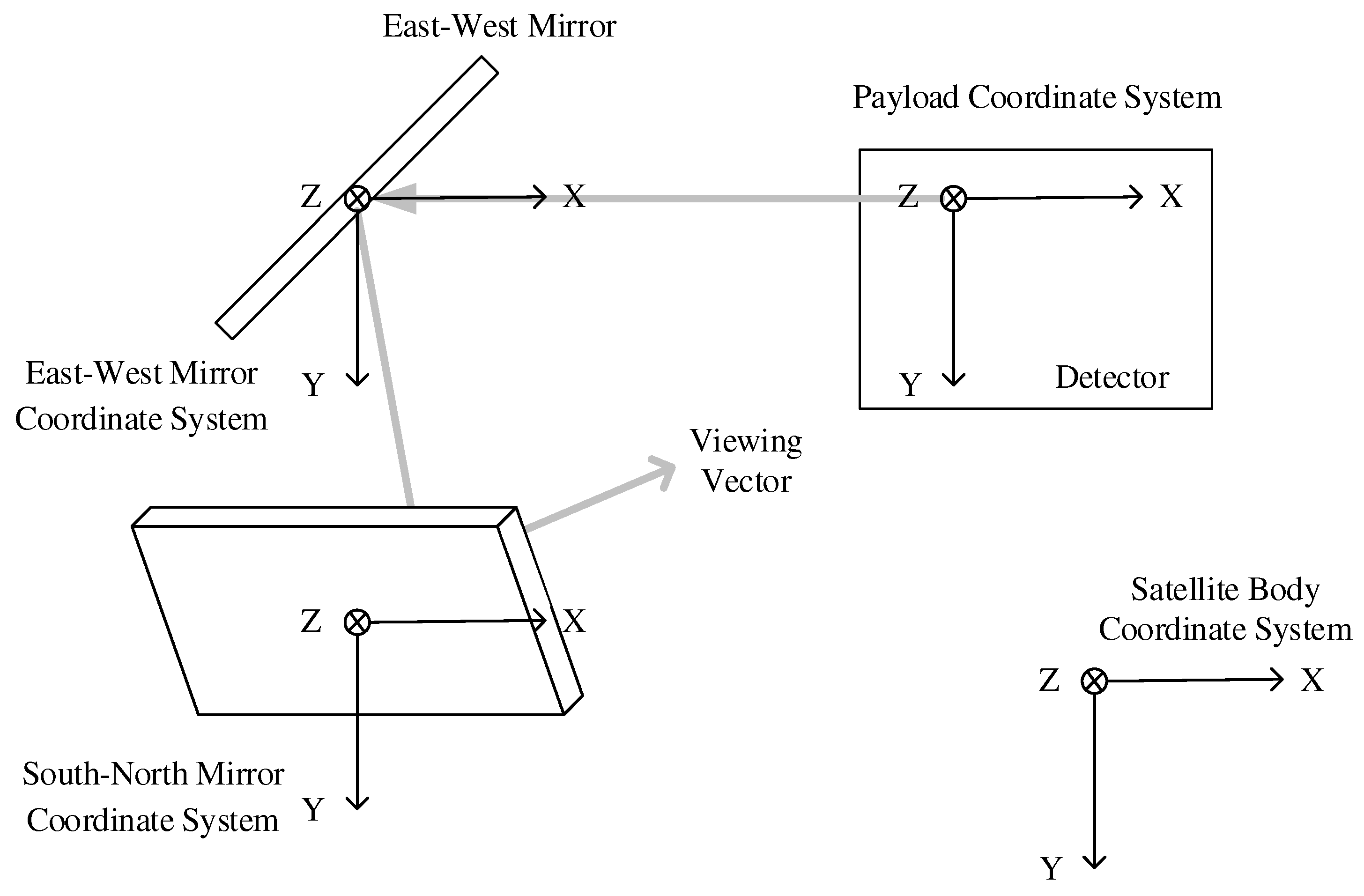
Figure 2.
Flowchart of the rapid geolocation process.

Figure 3.
Flowchart of the Rapid Geolocation Algorithm.
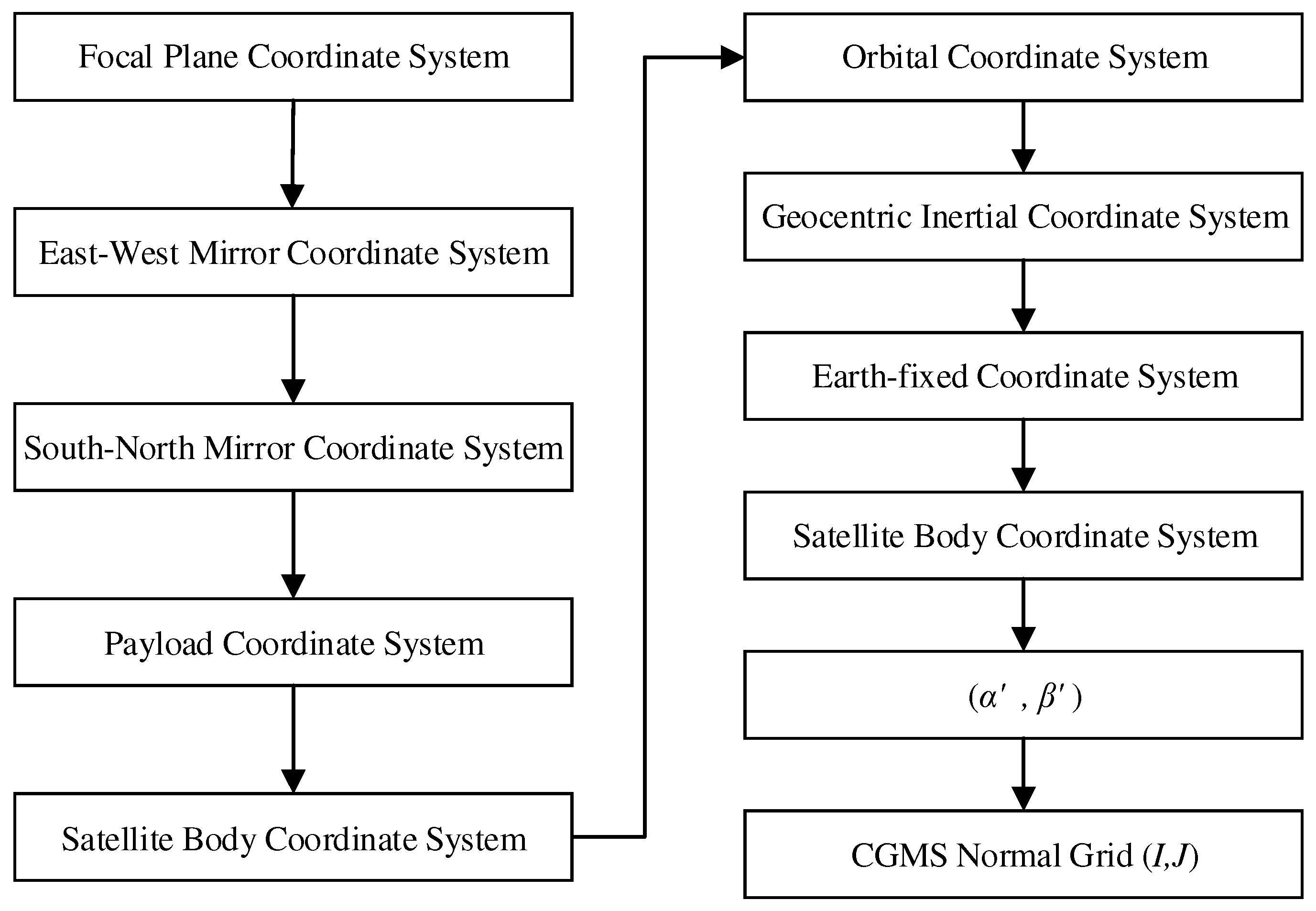
Figure 4.
Comparison of Geolocation Results of the Two Geolocation Processes at the Satellite Subpoint.
Figure 4.
Comparison of Geolocation Results of the Two Geolocation Processes at the Satellite Subpoint.
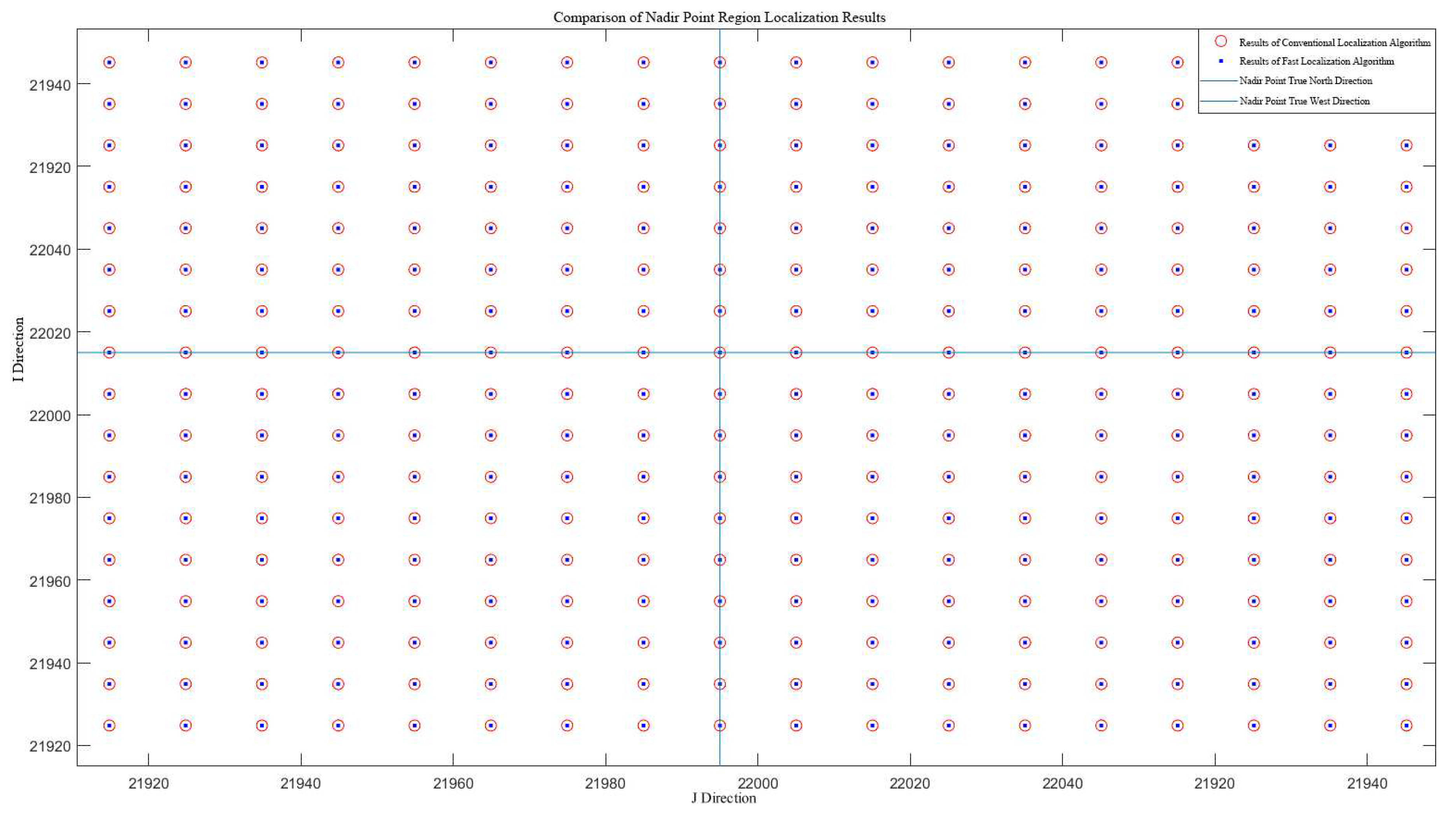
Figure 5.
Comparison of Geolocation Results of the Two Geolocation Processes at the Western Edge of the Earth.
Figure 5.
Comparison of Geolocation Results of the Two Geolocation Processes at the Western Edge of the Earth.

Figure 6.
Comparison of Geolocation Results of the Two Geolocation Processes at the Northern Edge of the Earth.
Figure 6.
Comparison of Geolocation Results of the Two Geolocation Processes at the Northern Edge of the Earth.
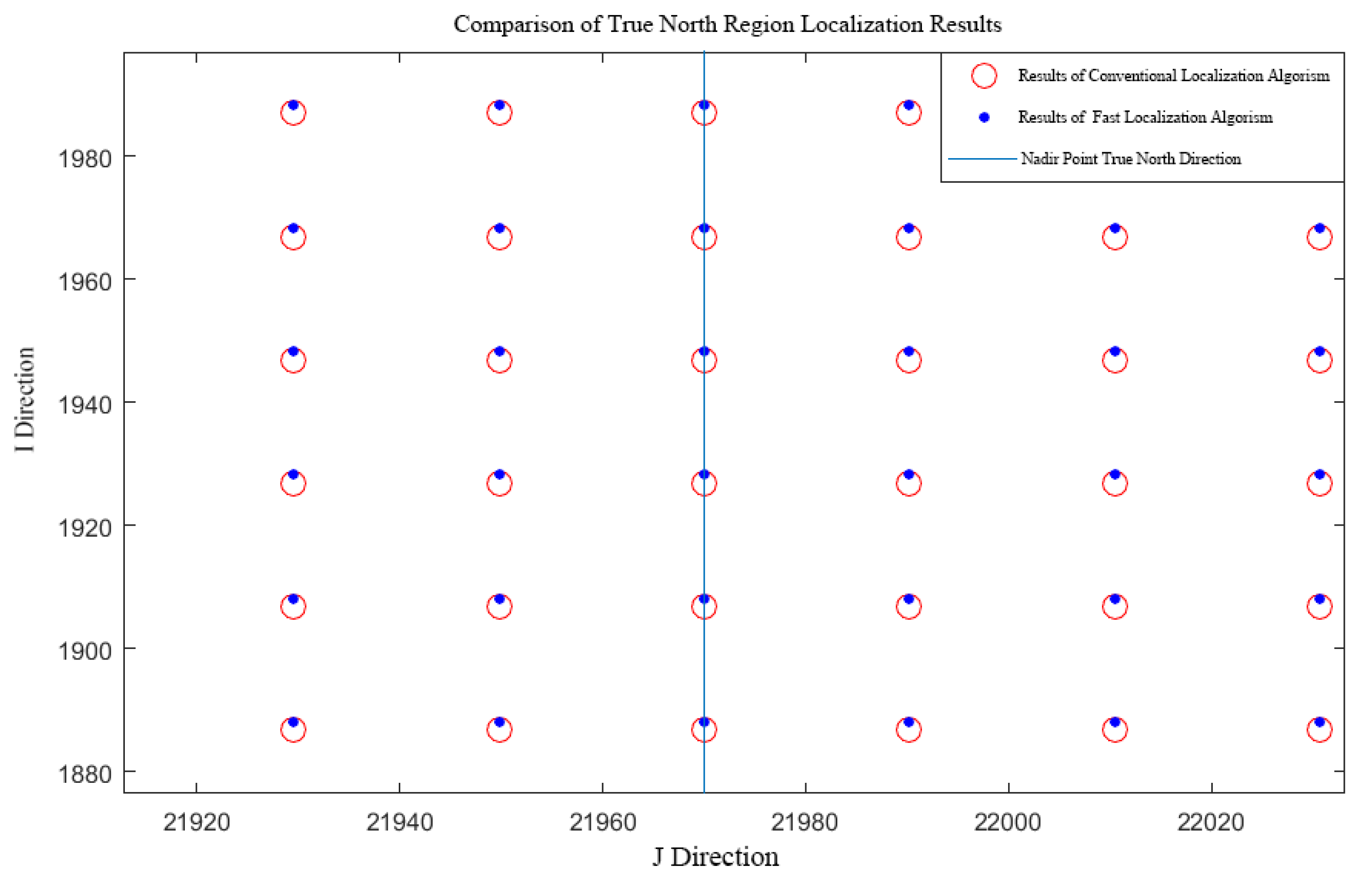

Table 1.
Comparison of selected param of geostationary satellites from the USA, Europe, China, and Japan.
Table 1.
Comparison of selected param of geostationary satellites from the USA, Europe, China, and Japan.
| Satellite Name | Spatial Resolution (km) | Full Disk Time (min) | Regional Scan Time (min) |
|---|---|---|---|
| GEOS-R | 0.5–2 | 5 | 1000×1000 km 2.5 min |
| Himawari-8/9 | 0.5–2 | 10 | Japan Region 2.5 min |
| MTG-I1 | 0.5–2 | 10 | Europe and North Africa 2.5 min |
| FY4-A | 0.5–4 | 15 | 2500×2500 km 3 min |
| FY4-B | 0.25–4 | 15 | 2000×2000 km 1 min |
Table 2.
Time Comparison of Two Geolocation Algorithms.
| Index | Coordinate Transformation | Conventional Method (ms) | Rapid Method (ms) |
|---|---|---|---|
| 1 | Focal plane to Payload | 563 | 563 |
| 2 | Payload to Satellite Body | 747 | 747 |
| 3 | Satellite Body to Orbital | 856 | 856 |
| 4 | Orbital to Earth-centered Inertial | 3119 | 3119 |
| 5 | Earth-centered Inertial to Earth-fixed | 17416 | 17416 |
| 6 | Earth-fixed to Geodetic | 20185 | N/A |
| 7 | Geodetic to IJ | 1374 | N/A |
| 8 | Rapid Geolocation Algorithm Earth-fixed to IJ | N/A | 1442 |
| Total | 44260 | 24143 |
Table 3.
Geolocation Differences in Different Test Regions.
| Test Region | Mean Difference in I | Mean Difference in J |
|---|---|---|
| Satellite Subpoint | 7.8125e-05 | 7.8125e-05 |
| Western Edge | 8.4570e-05 | 0.0698 |
| Northern Edge | 0.0697 | 9.1992e-05 |
Disclaimer/Publisher’s Note: The statements, opinions and data contained in all publications are solely those of the individual author(s) and contributor(s) and not of MDPI and/or the editor(s). MDPI and/or the editor(s) disclaim responsibility for any injury to people or property resulting from any ideas, methods, instructions or products referred to in the content. |
© 2023 by the authors. Licensee MDPI, Basel, Switzerland. This article is an open access article distributed under the terms and conditions of the Creative Commons Attribution (CC BY) license (http://creativecommons.org/licenses/by/4.0/).
Copyright: This open access article is published under a Creative Commons CC BY 4.0 license, which permit the free download, distribution, and reuse, provided that the author and preprint are cited in any reuse.


