Inference of Stress-Strength Reliability Based on Adaptive Progressive Type-II Censing from Bath Tube Distribution with Application to Carbon Fiber Data

Preprint

Article

Inference of Stress-Strength Reliability Based on Adaptive Progressive Type-II Censing from Bath Tube Distribution with Application to Carbon Fiber Data

Altmetrics

Downloads

116

Views

Comments

Essam A. Ahmed^*

This version is not peer-reviewed

Submitted:

22 December 2023

Posted:

26 December 2023

You are already at the latest version

Alerts

Abstract

In this paper, we will use the maximum likelihood estimation (MLE) and the Bayes methods to perform estimation procedures for the reliability of stress-strength ℜ=P[X>Y] based on independent adaptive progressive censored samples that were taken from the Chen distributions. An approximate confidence interval of ℜ is constructed using a variety of classical techniques, such as the normal approximation of the MLE, the normal approximation of the log-transformed MLE, and the percentile bootstrap (Boot-p) procedure. The Bayesian estimation of ℜ is obtained based on the balanced loss function, which comes in two versions here, the symmetric balanced squared error (BSE) loss function and the asymmetric balanced linear exponential (BLINEX) loss function. When estimating ℜ using the Bayesian approach, all the unknown parameters of the Chen distributions are assumed to be independently distributed and to have informative gamma priors. Further, a mixture of Gibbs sampling algorithm and Metropolis-Hastings algorithm is used to compute the Bayes estimate of ℜ and the associated highest posterior density credible interval. In the end, simulation research are used to assess the general overall performance of the proposed estimators and a real data set is provided to exemplify the theoretical results.

Keywords:

Subject: Computer Science and Mathematics - Mathematics

MSC: 62N02; 62F10; 62F15

1. Introduction

Modern industrial systems are frequently created with exacting criteria of quality. There are many different methods used to improve system reliability. A redundant structure is a method for further developing system reliability. For instance, a cloud storage server typically has a minimum of one backup to assist users in protecting sensitive data. In the same vein, a commercial aircraft is equipped with a backup engine for use in the event of unexpected malfunctions. In many industrial products, such as production systems, pump systems, power generation systems, etc. The reliability of systems is impacted by a number of factors when they are added to be used within the actual environment, including operating environments, outdoor shocks, operators, and so on. One way to look at these factors is as stresses the system experiences while it is operating. In such situations, the stress-strength (S-S) model is normally used to evaluate the parallel machine’s reliability. The S-S version, first offered through Birnbaum and McCarty (1958), is one of the most widely used reliability fashions. For this model, it fails if its stress exceeds its strength. Therefore, device reliability can be described as the probability that the device’s strength exceeds its stress. That is expressed mathematically in the form

ℜ = P (Y < X)

, where X stands for the stress variable and Y for the system’s strength. Numerous statistical issues, including those involving quality control, engineering, clinical, and biostatistics, have found use for the S-S model. In the context of medical research, for instance, the variable ℜ quantifies the efficacy of a novel treatment in relation to its control; in this case, X and Y stand for the new treatment’s and the control’s respective effects. Similar to this, in engineering studies, ℜ stands for the likelihood that a system component’s strength (Y) will exceed the system’s external stress (X). An overview of all the techniques and consequences related to the S-S version is provided by Kotz et al. (2003).

Evaluating the reliability of the S-S model using different statistical techniques has been the focus of a lot of research lately. For example, Gittani et al. (2015) presented point and interval estimates of the reliability of the S-S model under a Lindley power distribution. They used maximum likelihood (ML) estimators as well as parametric and nonparametric bootstrapping techniques. Using recorded samples from two parameter generalized exponential distribution, Asgharzadeh et al. (2017) estimated the S-S model

P (Y < X)

. The process of establishing a generalized inference on the S-S model based on the unknown parameters of the generalized exponential distribution was carried out by Wang et al. (2018). With the growing interest in this system and the importance of Chen distribution, which has become evident in the past two decades, in order to obtain point and interval estimates for a multicomponent ℜ of an S-out-of-j system, Kayal et al. (2020) used classical and Bayesian methods under the assumption that both the S-S variables follow a Chen distribution with a common shape parameter. The reliability estimation of ℜ when the failure times are progressively Type-II censored and both the latent strength and stress variables originate from the inverse exponential Rayleigh distribution was discussed by Ma et al. (2023). Moreover, Agiwal (2023) developed a Bayesian estimation method to estimate ℜ where X and Y are inverse Chen random variables. Recently, Sarhan and Tolba (2023) have given attention to the estimation of ℜ for step-stress partial acceleration life testing, when the stress and strength additives are independent random variables generated from Weibull distributions with specific shape and scale parameters.

To gather information about the lifetime and reliability characteristics of products, various units are typically used during life testing experiments. In actuality, it is sometimes not possible to finish experiments until all failures are noted due to time and financial constraints. To increase test efficiency in this regard, several censoring schemes and testing techniques are suggested. In practise, the most commonly used methods in the literature are type I and type II control. According to these methods, life tests terminate or stop after a specified time or a specified number of failures, respectively. Through various life testing experiments, there are many different challenges that experimenters face in order to be able to control the testing time as well as keep the experimental units intact, so stopping the experiment before all experimental units fail is one of the solutions to achieve these goals. This is done through the use of control structures that rely on deferring some active devices from the experiment. The progressive censoring system is considered one of the experimental designs commonly used in recent years, as through this system, survival units are arbitrarily removed from the test at any stage of the test. As a result, it is more adaptable and efficient than conventional censoring techniques. Over time, numerous models of progressive censorship have been discussed. According to this model, censoring has been divided into two parts: when the experiment ends after a specific time, this section is called progressive censoring of the first type, while the second part is progressive censoring of the second type, and in this section the experiment stops after a predetermined number of failures appear. Through both sections, experimenters will be able to freely remove test units during the experiment at non-terminal times. Whithin a type-II progressive censoring scheme, to test the life of units, the experimenter puts n units through the test at time zero, and only m units that fail completely are observed. With the primary failure, which may take the shape

X_{1}

R_{1}

is randomly eliminated from the final devices within the test. At the time of the second failure

X_{2}

, the experimenter selects a random number of final units, let it be

R_{2}

, and they are removed from the experiment. Finally, in the same sequence, at the time of the mth failure,

X_{m}

the experimenter removes all remaining units

R_{m}

from the experiment, where

R_{m} = n - m - \sum_{i = 1}^{m - 1} R_{i} .

When test units are highly reliable, the long testing time represents one of the main drawbacks of the progressive type-II censoring model. For this reason, Ng et al. (2009) suggested an improved model (see Figure 1) that allows for adjustments to the censoring scheme throughout the experiment. This improved model is known in the literature as the adaptive type-II progressive censoring model. The technique of this model can be explained as follows.

(1) First, the effective sample size m, the number of units to be tested n, the progressive censoring scheme (

R_{1}, R_{2}, . . ., R_{m}

) and the time point T must be determined in advance before the beginning of the experiment.

(2) As indicated by the preceding progressive censoring strategy,

R_{1}

units are arbitrarily eliminated from the test at the moment of the first failure

X_{1 : m : n}

R_{2}

units are also arbitrarily removed from the test at the moment of the second failure,

X_{2 : m : n}

, and so on.

(3) When the mth failure occurs before time T (i.e.,

X_{m : m : m} < T

), the test ends at this point with the unchanged progressive censoring scheme (

R_{1}, R_{2}, . . ., R_{m}

), and we will have the standard progressive type-II censoring. with the unchanged progressive censoring scheme (

R_{1}, R_{2}, . . ., R_{m}

). Where

R_{m} = n - m - \sum_{i = 1}^{m} R_{i} .

(4) In the event where

X_{J : m : n} < T < X_{J + 1 : m : n}

, where

J < m

and

X_{J : m : n}

is the Jth failure time occur before the time T, then no surviving item will be removed from the test by placing

R_{J + 1} = R_{J + 2} = . . . = R_{m - 1} = 0

, and at the time

X_{m : m : n}

all remaining units

R_{m}^{*}

are removed, where

R_{m}^{*} = n - m - \sum_{i = 1}^{J} R_{i}

. Because of this, the progressive censoring scheme that is being used in this instance is (

R_{1}, R_{2}, . . ., R_{J}, 0, 0, . . ., 0, n - m - \sum_{i = 1}^{J} R_{i}

(5) After running the previously specified test, we may get the following adaptive progressive type-II censored observation data

\{\begin{matrix} (X_{1 : m : n}, R_{1}), (X_{2 : m : n}, R_{2}), . . ., (X_{m : m : n}, R_{m}) if X_{m : m : n} < T, R_{m} = n - m - \sum_{i = 1}^{m} R_{i}, \\ (X_{1 : m : n}, R_{1}), . . ., (X_{J : m : n}, R_{J}), (X_{J + 1 : m : n}, 0), . . ., (X_{m : m : n}, R_{m}^{*}) if X_{J : m : n} < T < X_{J + 1 : m : n}, J < m . \end{matrix}

More works presented on the adaptive type-II progressive censoring model, we referred to Almuqrin et al. (2023) and the references contained within it.

Many scientific and engineering applications use a variety of distributions, including gamma, exponential, Rayleigh, normal, Weibull, and others, to model the lifetime characteristic of products. Among the various probabilistic models, bathtub-shaped failure rate distributions have drawn a lot of attention. These models are highly helpful for studying complex systems or sub-systems and for making decisions, particularly when the target product’s entire life cycle needs to be modelled. Regarding this, numerous authors have proposed and discussed in literature a variety of probability models featuring bathtub-shaped failure rate functions. The bathtub-shaped hazard function offers a suitable conceptual model for the lifespan of humans as well as certain mechanical and electronic products. Xie and Lai (1995), Wang (2002), and Xie et al. (2002) are only a few of the writers whose articles contain references to the earlier comprehensive work on parametric probability distributions with bathtub-shaped failure rate function. The Chen distribution is considered one of the most important distributions that contain bathtub curves.

Chen (2000) introduced a distribution that is often called the Chen or bathtub-shaped distribution with two parameters in the literature. It is a significant probability model that is frequently applied to lifetime analysis. This probability model is truly crucial for studying physical events for which the hazard rate function predicts bathtub-shaped behavior. It gives complex systems whose failure rates vary over time a flexible way to be modelled. One of the primary features of the Chen distribution is its bathtub-shaped failure rate curve, which has three unique phases (decreasing, constant, and ascending) and may be used to describe a wide range of systems. This curve has a wide range of potential applications, including researching the efficacy of medications or therapies across various age groups. It can be helpful when analyzing mortality data as well. When modeling the reliability of items or systems that are prone to wear and tear, one might employ the Chen distribution. The following are the cumulative density function (CDF) and probability density function (PDF) for the Chen distribution:

F (x; α, β) = 1 - exp [α (1 - e^{x^{β}})], x > 0, α > 0, β > 0

(1)

and

f (x; α, β) = α β x^{β - 1} exp [x^{β} + α (1 - e^{x^{β}})], x > 0, α > 0, β > 0,

(2)

Here, both

α

and

β

are known as shape parameters. As for the hazard rate function (HRF) for the Chen distribution, it is given in the following form

H (x; α, β) = α β x^{β - 1} exp [x^{β}], x > 0,

(3)

The Chen distribution’s HRF (3) has a bathtub form with a minimum at

{(\frac{1 - β}{β})}^{1 / β}

, when

β < 1

. It increases when

β \geq 1

. This distribution may be used to describe many kinds of failure-time data quite well since it is fairly adaptable. For example, if we select

β = 1

in (1), this distribution further transforms into a Gompertz distribution with parameters 1 and

α

. When

α = 1

, the exponential power distribution results. If

x \sim

Chen(

α, β

) and we take

Y = {(e^{x^{β}} - 1)}^{1 / θ}

, the distribution turns into a Weibull distribution with parameters

α

and

θ

Compared to other two-parameter models, this distribution stands out due to a few key features, including a bathtub-shaped hazard rate function and closed-form joint confidence regions and shape parameter confidence intervals. As a result, researchers have paid close attention to this distribution in recent years due to its broad applicability in simulating a variety of real-life phenomena. For a brief review, Using progressive type-II censoring, Wu (2008) calculated the MLEs of the unknown parameters and approximated their intervals. Rastogi, Tripathi, and Wu (2012) achieved the Bayesian inference of this distribution against various symmetric and asymmetric loss functions. Using the likelihood and Bayes approaches, Sarhan et al. (2015) determined the reliability

ℜ = P (Y < X)

where X and Y are two independent r.v.s. with a two-parameter Chen distribution. Tarvirdizade and Ahmadpour (2016), and Raqab et al. (2018) have studied the estimation of the S-S reliability for the two-parameter Chen model based on upper record values. Using data that was progressively censored, Kayal et al. (2017) looked at the Bayesian one and two sample prediction. Ahmed et al. (2020) observed the Chen distribution for a competitive risk model with progressive type-II censored data. The S-S reliability of this lifespan distribution was investigated by Shoaee and Khorram (2015) using type-II progressively censored data. According to recent observations by Wang et al. (2022) the multicomponent system is reliable when both stress and strength follow Chen distribution.

One significant phenomenon in life testing studies that we mention is the S-S models. While there is a large body of literature on the inference processes of S-S models under full samples, little emphasis has been given to the case of censored data, specifically type II adaptive progressive censored data. From this, our objective became clear. This article’s primary goal is to use adaptive progressive type censored data to estimate the S-S Reliability ℜ, in the case when X and Y are Chen distributions’ independent variables.

The following describes the paper’s methodology: First, we’ll estimate ℜ using the ML technique. Next we will discuss the asymptotic confidence interval of ℜ. The delta approach is used to estimate the variance of the ℜ estimator in order to achieve the required interval. Second, the balanced loss function is taken into account in order to compute Bayesian estimates of ℜ, with special attention paid to the balanced square error (BLINEX) loss function (BSEL) and the balanced exponential loss function. In the last ten years, the Markov chain Monte Carlo technique has become a popular solution to the Bayesian approach to deal with the problem of many integrals arising in the posterior distribution. Using this technique, we calculate the Bayes estimates and credible intervals for ℜ. A comprehensive numerical comparison of the presented estimates with respect to means squared errors, coverage probabilities, and confidence lengths is carried out.

The structure of the paper is as follows after this introduction. Section 2: Here, we give the expression for ℜ of Chen distribution. The ML estimate of ℜ and the associated approximate confidence interval as will as boot-p confidence interval are also discussed. In Section 3, we derive the Bayesian estimate ℜ and the its credible interval using the Gibbs technique within Metropolis-Hastings. In Section 6 we present an examination of an actual data set. In Section 5, we do a Monte Carlo simulation analysis to compare the suggested values of ℜ. In Section 6, we finally bring the article to a close.

2. Maximum Likelihood Estimation of ℜ

Given independent strength and stress random variables X and Y that have parameters (

α_{1}, β

) and (

α_{2}, β

) correspondingly, according to Chen distributions, the reliability of the component is defined as

\begin{matrix} ℜ & = & P (X \geq Y) = P (S t r e s s > S t r e n g t h) = \\ = & \int_{0}^{\infty} α_{1} β w^{β - 1} e^{w^{β}} e^{α_{1} (1 - e^{w^{β}})} [1 - e^{α_{2} (1 - e^{w^{β}})}] d w \\ = & 1 - α_{1} \int_{0}^{\infty} β w^{β - 1} e^{w^{β}} e^{(α_{1} + α_{2}) (1 - e^{w^{β}})} d w = \frac{α_{2}}{α_{1} + α_{2}} . \end{matrix}

(4)

It is worth noting that the evaluation depends on whether this probability (

ℜ = P (X \geq Y)

) is less than or greater than

0.5

. The result is evaluated and interpreted as follows:

- The lifetime of the two products or any two units is equal if

ℜ = 0.5

- If

ℜ > 0.5

, the lifetime of Unit/Product 1 exceeds that of Unit/Product 2. For example, if

ℜ = 0.7

, Unit/Product 1 is better than Unit/Product 2 with a probability of 70%.

- If ℜ < 0.5, the lifetime of Unit/Product 2 exceeds that of Unit/Product 1. For example, if

ℜ = 0.20

, Unit/Product 2 is better than Unit/Product 1 with a

80 %

probability (

1 - 0.20 = 0.9

). The adaptive type-II censored sample is used in this part to determine the MLE of ℜ.Since ℜ is independent of the common shape parameter

β

in this case, obtaining ℜ is a straightforward process using Equation (4) provided that the values of the parameters

α_{1}

and

α_{2}

are known or estimated using different estimation methods.

Suppose

X = (X_{1 : m_{1} : n_{1}}, X_{2 : m_{1} : n_{1}}, . . ., X_{m_{1} : m_{1} : n_{1}})

is an adaptive type-II progressive censored sample from Ch(

α_{1}, β

) with the scheme {

m_{1}, n_{1}, T_{1}, R_{1}, R_{2}, . . ., R_{m_{1}}

} such that

X_{J_{1} : m_{1} : n_{1}} < T_{1} < X_{J_{1} + 1 : m_{1} : n_{1}}

. Additionally,

Y = (Y_{1 : m_{2} : n_{2}}, Y_{2 : m_{2} : n_{2}}, . . ., Y_{m_{2} : m_{2} : n_{2}})

be an adaptive type-II progressive censored sample from Ch(

α_{2}, β

) under the scheme {

m_{2}, n_{2}, T_{2}, S_{1}, S_{2}, . . ., S_{m_{2}}

} such that

Y_{J_{2} : m_{2} : n_{2}} < T_{2} < Y_{J_{2} + 1 : m_{2} : n_{2}}

According to the two independent random samples X and Y, the likelihood function (LF) is provided by

L (Θ d a t a) = \{C_{J_{1}} \prod_{i = 1}^{m_{1}} f (x_{i}) \prod_{i = 1}^{J_{1}} {[\bar{F} (x_{i})]}^{R_{i}} {[\bar{F} (x_{m_{1}})]}^{R_{m_{1}}^{*}}\} \{C_{J_{2}} \prod_{j = 1}^{m_{2}} f (y_{j}) \prod_{j = 1}^{J_{2}} {[\bar{F} (y_{j})]}^{S_{i}} {[\bar{F} (y_{m_{2}})]}^{S_{m_{2}}^{*}}\},

(5)

where

C_{J_{1}} = \prod_{i = 1}^{m_{1}} (m_{1} - i + 1 - \sum_{k = 1}^{max {i - 1, J_{1}}} R_{k},), C_{J_{2}} = \prod_{j = 1}^{m_{2}} (m_{2} - j + 1 - \sum_{l = 1}^{max {j - 1, J_{2}}} S_{l},

and

R_{m}^{*} = n_{1} - m_{1} - \sum_{i = 1}^{J_{1}} R_{i}, S_{m}^{*} = n_{2} - m_{2} - \sum_{j = 1}^{J_{2}} S_{j}, and \bar{F} (\cdot) = 1 - F (\cdot) .

Wu (2015) provides the likelihood function (5) for ℜ in the progressive censored sample case, which is produced in the situation

T_{1} = T_{1} = \infty

. Moreover, the likelihood function for ℜ in the complete sample is reached when

T_{1} = T_{1} = \infty

and

R_{i} = S_{i} = 0

, as reported by Sarhan et al. (2015).

The following may be used to represent the LF for the observed sample data, X and Y, using Equations (1), (2), and (5):

\begin{matrix} L (Θ d a t a) & = & C_{J_{1}} C_{J_{2}} α_{1}^{m_{1}} α_{2}^{m_{2}} β^{m_{1} + m_{2}} exp \{α_{1} R_{m_{1}}^{*} (1 - e^{x_{m_{1}}^{β}}) + α_{2} S_{m_{2}}^{*} (1 - e^{y_{m_{2}}^{β}})\} \prod_{i = 1}^{m_{1}} x_{i}^{β - 1} \prod_{j = 1}^{m_{2}} y_{j}^{β - 1} \\ \times exp \{\sum_{i = 1}^{m_{1}} [x_{i}^{β} + α_{1} (1 - e^{x_{i}^{β}})] + \sum_{j = 1}^{m_{2}} [y_{j}^{β} + α_{2} (1 - e^{y_{j}^{β}})]\} . \\ \times exp \{α_{1} \sum_{i = 1}^{J_{1}} R_{i} (1 - e^{x_{i}^{β}}) + α_{2} \sum_{j = 1}^{J_{2}} S_{j} (1 - e^{y_{j}^{β}})\} \end{matrix}

(6)

Ignoring the additive constants

C_{J_{1}}

and

C_{J_{2}}

, the log-LF, say

L

log L (Θ d a t a)

(

Θ = (α_{1}, α_{2}, β)

) is given by:

\begin{matrix} L & = & m_{1} log [α_{1}] + m_{2} log [α_{2}] + (m_{1} + m_{2}) log [β] + (β - 1) [\sum_{i = 1}^{m_{1}} log (x_{i}) + \sum_{j = 1}^{m_{2}} log (y_{j})] \\ + \sum_{i = 1}^{m_{1}} [x_{i}^{β} + α_{1} (1 - e^{x_{i}^{β}})] + \sum_{j = 1}^{m_{2}} [y_{j}^{β} + α_{2} (1 - e^{y_{j}^{β}})] \\ + \sum_{i = 1}^{J_{1}} α_{1} [R_{i} (1 - e^{x_{i}^{β}}) + R_{m_{1}}^{*} (1 - e^{x_{m_{1}}^{β}})] + \sum_{j = 1}^{J_{2}} α_{2} [S_{j} (1 - e^{y_{j}^{β}}) + S_{m_{2}}^{*} (1 - e^{y_{m_{2}}^{β}})] . \end{matrix}

(7)

The first order derivatives of the log-likelihood function, with respect to

α_{1}

α_{2}

and

β

are

\frac{\partial L}{\partial α_{1}} = \frac{m_{1}}{α_{1}} + \sum_{i = 1}^{m_{1}} (1 - e^{x_{i}^{β}}) + \sum_{i = 1}^{J_{1}} R_{i} (1 - e^{x_{i}^{β}}) + R_{m_{1}}^{*} (1 - e^{x_{m_{1}}^{β}}) = 0,

(8)

\frac{\partial L}{\partial α_{2}} = \frac{m_{2}}{α_{2}} + \sum_{j = 1}^{m_{2}} (1 - e^{y_{j}^{β}}) + \sum_{j = 1}^{J_{2}} S_{j} (1 - e^{y_{j}^{β})} + S_{m_{2}}^{*} (1 - e^{y_{m_{2}}^{β}}) = 0,

(9)

and

\begin{matrix} \frac{\partial L}{\partial β} = \frac{(m_{1} + m_{2})}{β} + \sum_{i = 1}^{m_{1}} log (x_{i}) + \sum_{j = 1}^{m_{2}} log (y_{j}) \\ + \sum_{i = 1}^{m_{1}} x_{i}^{β} log (x_{i}) (1 - α_{1} e^{x_{i}^{β})} - α_{1} [\sum_{i = 1}^{J_{1}} R_{i} x_{i}^{β} log (x_{i}) e^{x_{i}^{β}} + x_{m_{1}}^{β} log (x_{m_{1}}) R_{m_{1}}^{*} e^{x_{m_{1}}^{β}}] \\ + \sum_{j = 1}^{m_{2}} y_{j}^{β} log (y_{i}) (1 - α_{2} e^{y_{j}^{β}}) - α_{2} [\sum_{j = 1}^{J_{2}} S_{j} y_{j}^{β} log (y_{j}) e^{y_{j}^{β}} + y_{m_{2}}^{β} log (y_{m_{2}}) S_{m_{2}}^{*} e^{y_{m_{2}}^{β}}] = 0, \end{matrix}

(10)

From (8) and (9), we obtain

{\hat{α}}_{1} (β) = \frac{m_{1}}{U (\underset{̲}{x}, β)}, and {\hat{α}}_{2} (β) = \frac{m_{2}}{V (\underset{̲}{x}, β)}

(11)

where,

U (\underset{̲}{x}, β) = \sum_{i = 1}^{m_{1}} (e^{x_{i}^{β}} - 1) + \sum_{i = 1}^{J_{1}} R_{i} (e^{x_{i}^{β}} - 1) + R_{m_{1}}^{*} (e^{x_{m_{1}}^{β}} - 1),

(12)

and

V (\underset{̲}{y}, β) = \sum_{j = 1}^{m_{2}} (e^{y_{j}^{β}} - 1) + \sum_{j = 1}^{J_{2}} S_{j} (e^{y_{j}^{β}} - 1) + S_{m_{2}}^{*} (e^{y_{m_{2}}^{β}} - 1),

(13)

In the case that the parameter

β

is known, the MLE of

α_{1}

and

α_{2}

can be obtained directory from the Equation (11). But, when the all parameters are unknown, the parameter

β

will be estimated by maximizing the profile log-likelihood function

L ({\hat{α}}_{1} (β), {\hat{α}}_{2} (β), β)

, with respect to

β

by solving the following nonlinear equation:

\begin{matrix} \frac{\partial L}{\partial β} & = & \frac{(m_{1} + m_{2})}{β} + [\sum_{i = 1}^{m_{1}} log (x_{i}) + \sum_{j = 1}^{m_{2}} log (y_{j})] + \sum_{i = 1}^{m_{1}} x_{i}^{β} log (x_{i}) [1 - \frac{m_{1} e^{x_{i}^{β}}}{U (\underset{̲}{x}, β)}] \\ + \sum_{j = 1}^{m_{2}} y_{j}^{β} log (y_{i}) [1 - \frac{m_{2} e^{y_{j}^{β}}}{V (\underset{̲}{y}, β)}] - \frac{m_{1} W (\underset{̲}{x}, β)}{U (\underset{̲}{x}, β)} - \frac{m_{2} Z (\underset{̲}{y}, β)}{V (\underset{̲}{y}, β)} = 0, \end{matrix}

(14)

where

W (\underset{̲}{x}, β) = [\sum_{i = 1}^{J_{1}} R_{i} x_{i}^{β} log (x_{i}) e^{x_{i}^{β}} + x_{m_{1}}^{β} log (x_{m_{1}}) R_{m_{1}}^{*} e^{x_{m_{1}}^{β}}],

(15)

and

Z (\underset{̲}{y}, β) = [\sum_{j = 1}^{J_{2}} S_{j} y_{j}^{β} log (y_{j}) e^{y_{j}^{β}} + y_{m_{2}}^{β} log (y_{m_{2}}) S_{m_{2}}^{*} e^{y_{m_{2}}^{β}}],

(16)

This non-linear Equation (14) has a fixed point solution at

\hat{β}

, which may be found by using the following straightforward iterative method

h (β_{(k)}) = β_{(k + 1)},

(17)

h (β) = \frac{- (m_{1} + m_{2})}{\sum_{i = 1}^{m_{1}} log (x_{i}) [1 + x_{i}^{β} (1 - \frac{m_{1} e^{x_{i}^{β}}}{U (\underset{̲}{x}, β)})] + \sum_{j = 1}^{m_{2}} log (y_{j}) [1 + y_{j}^{β} (1 - \frac{m_{2} e^{y_{j}^{β}}}{V (\underset{̲}{y}, β)})] - \frac{m_{1} W (\underset{̲}{x}, β)}{U (\underset{̲}{x}, β)} - \frac{m_{2} Z (\underset{̲}{y}, β)}{V (\underset{̲}{y}, β)}} .

(18)

Where, The kth iteration of

\hat{β}

is denoted by

β_{(k)}

. The process of iteration ought to be terminated when

| β_{(k)} - β_{(k + 1)}

| is small enough.

Equation (11) may now be used to get

{\hat{α}}_{1}

and

{\hat{α}}_{2}

{\hat{α}}_{1} (\hat{β})

and

{\hat{α}}_{2} (\hat{β})

, respectively, by using

\hat{β}

. An easy way to obtain MLE

{\hat{ℜ}}_{M L}

of ℜ is to use the invariant properties of MLEs. Afterwards,

{\hat{ℜ}}_{M L}

is obtained from (4) as follows:

\begin{matrix} {\hat{ℜ}}_{M L} & = & \frac{{\hat{α}}_{2} (\hat{β})}{{\hat{α}}_{1} (\hat{β}) + {\hat{α}}_{2} (\hat{β})} = m_{2} {[m_{2} + m_{1} \frac{V (\underset{̲}{y}, \hat{β})}{U (\underset{̲}{x}, \hat{β})}]}^{- 1} \\ = & m_{2} {[m_{2} + m_{1} \frac{\sum_{j = 1}^{m_{2}} (e^{y_{j}^{\hat{β}}} - 1) + \sum_{j = 1}^{J_{2}} S_{j} (e^{y_{j}^{\hat{β}}} - 1) + S_{m_{2}}^{*} (e^{y_{m_{2}}^{\hat{β}}} - 1)}{\sum_{i = 1}^{m_{1}} (e^{x_{i}^{\hat{β}}} - 1) + \sum_{i = 1}^{J_{1}} R_{i} (e^{x_{i}^{\hat{β}}} - 1) + R_{m_{1}}^{*} (e^{x_{m_{1}}^{\hat{β}}} - 1)}]}^{- 1} . \end{matrix}

(19)

2.1. Asymptotic Confidence Interval of ℜ

Here, we construct asymptotic confidence interval (ACI) of ℜ using the asymptotic distribution of MLE ℜ for which we also require asymptotic distribution of

Θ = ({\hat{α}}_{1}, {\hat{α}}_{2}, \hat{β})

. In this regard, the Fisher information matrix

I (α_{1}, α_{2}, β)

is written as

I (α_{1}, α_{2}, β) = E [\begin{matrix} l l l - \frac{\partial^{2} ℓ}{\partial α_{1}^{2}} & - \frac{\partial^{2} ℓ}{\partial α_{1} \partial α_{2}} & - \frac{\partial^{2} ℓ}{\partial α_{1} \partial β} \\ - \frac{\partial^{2} ℓ}{α_{2} \partial α_{1}} & - \frac{\partial^{2} ℓ}{\partial α_{2}^{2}} & - \frac{\partial^{2} ℓ}{α_{2} \partial β} \\ - \frac{\partial^{2} ℓ}{\partial β \partial α_{1}} & - \frac{\partial^{2} ℓ}{\partial β \partial α_{2}} & - \frac{\partial^{2} ℓ}{\partial β^{2}} \end{matrix}],

and from the log-likelihood function (7), we have the second partial of

L

with respect to

α_{1}, α_{2}

, and

β

which is illustrated in the following

\begin{matrix} \frac{\partial^{2} L}{\partial α_{1}^{2}} & = & - \frac{m_{1}}{α_{1}^{2}}, \frac{\partial^{2} L}{\partial α_{2}^{2}} = - \frac{m_{2}}{α_{2}^{2}}, \\ \frac{\partial^{2} L}{\partial α_{1} \partial β} & = & \frac{\partial^{2} L}{\partial β \partial α_{1}} = - \sum_{i = 1}^{m_{1}} x_{i}^{β} e^{x_{i}^{β}} log x_{i} - \sum_{i = 1}^{J_{1}} R_{i} x_{i}^{β} e^{x_{i}^{β}} log x_{i} - R_{m_{1}}^{*} x_{m_{1}}^{β} e^{x_{m_{1}}^{β}} log x_{m_{1}}, \\ \frac{\partial^{2} L}{\partial α_{2} \partial β} & = & \frac{\partial^{2} L}{\partial β \partial α_{2}} = - \sum_{j = 1}^{m_{2}} y_{j}^{β} e^{y_{j}^{β}} log y_{j} - \sum_{j = 1}^{J_{2}} S_{j} y_{j}^{β} e^{y_{j}^{β}} log y_{j} - S_{m_{2}}^{*} y_{m_{2}}^{β} e^{y_{m_{2}}^{β}} log y_{m 2}, \end{matrix}

and

\begin{matrix} \frac{\partial^{2} L}{\partial β^{2}} & = & - \frac{(m_{1} + m_{2})}{β} - \sum_{i = 1}^{m_{1}} x_{i}^{β} {log}^{2} (x_{i}) {α_{1} e^{x_{i}^{β}} (1 + x_{i}^{β}) - 1} - \sum_{j = 1}^{m_{2}} y_{i}^{β} {log}^{2} (y_{i}) {α_{1} e^{y_{i}^{β}} (1 + y_{i}^{β}) - 1} \\ - α_{1} [\sum_{i = 1}^{J_{1}} R_{i} x_{i}^{β} {log}^{2} (x_{i}) e^{x_{i}^{β}} (1 + x_{i}^{β}) + R_{m_{1}}^{*} x_{m_{1}}^{β} {log}^{2} (x_{m_{1}}) e^{x_{m_{1}}^{β}} (1 + x_{m_{1}}^{β})] \\ - α_{2} [\sum_{j = 1}^{J_{2}} S_{j} y_{j}^{β} {log}^{2} (y_{j}) e^{y_{j}^{β}} (1 + y_{j}^{β}) + S_{m_{2}}^{*} y_{m_{2}}^{β} {log}^{2} (y_{m_{2}}) e^{y_{m_{2}}^{β}} (1 + y_{m_{2}}^{β})] . \end{matrix}

The above expectation is not easily expressed precisely, as is evident. Consequently, instead of using expectation, the observed Fisher information matrix will be employed. Given an MLE of (

α_{1}, α_{2}, β

) as (

{\hat{α}}_{1}, {\hat{α}}_{2}, \hat{β}

), the observed Fisher information matrix

I ({\hat{α}}_{1}, {\hat{α}}_{2}, \hat{β})

may be expressed as follows:

I ({\hat{α}}_{1}, {\hat{α}}_{2}, \hat{β}) = {[\begin{matrix} c c c - \frac{\partial^{2} L}{\partial α_{1}^{2}} & - \frac{\partial^{2} L}{\partial α_{1} \partial α_{2}} & - \frac{\partial^{2} L}{\partial α_{1} \partial β} \\ - \frac{\partial^{2} L}{α_{2} \partial α_{1}} & - \frac{\partial^{2} L}{\partial α_{2}^{2}} & - \frac{\partial^{2} L}{α_{2} \partial β} \\ - \frac{\partial^{2} L}{\partial β \partial α_{1}} & - \frac{\partial^{2} L}{\partial β \partial α_{2}} & - \frac{\partial^{2} L}{\partial β^{2}} \end{matrix}]}_{(α_{1}, α_{2}, β) = ({\hat{α}}_{1}, {\hat{α}}_{2}, \hat{β})} .

In accordance with this, the following is an estimated approximate covariance matrix of (

{\hat{α}}_{1}, {\hat{α}}_{2}, \hat{β}

\begin{matrix} [\begin{matrix} c c c V a r ({\hat{α}}_{1}) & C o v ({\hat{α}}_{1}, {\hat{α}}_{2}) & C o v ({\hat{α}}_{1}, \hat{β}) \\ C o v ({\hat{α}}_{2}, {\hat{α}}_{1}) & V a r ({\hat{α}}_{2}) & C o v ({\hat{α}}_{2}, \hat{β}) \\ C o v (\hat{β}, {\hat{α}}_{1}) & C o v (\hat{β}, {\hat{α}}_{2}) & V a r \hat{β}) \end{matrix}] = I^{- 1} ({\hat{α}}_{1}, {\hat{α}}_{2}, \hat{β}) \\ = {[\begin{matrix} c c c - \frac{\partial^{2} L}{\partial α_{1}^{2}} & - \frac{\partial^{2} L}{\partial α_{1} \partial α_{2}} & - \frac{\partial^{2} L}{\partial α_{1} \partial β} \\ - \frac{\partial^{2} L}{α_{2} \partial α_{1}} & - \frac{\partial^{2} L}{\partial α_{2}^{2}} & - \frac{\partial^{2} L}{α_{2} \partial β} \\ - \frac{\partial^{2} L}{\partial β \partial α_{1}} & - \frac{\partial^{2} L}{\partial β \partial α_{2}} & - \frac{\partial^{2} L}{\partial β^{2}} \end{matrix}]}_{(α_{1}, α_{2}, β) = ({\hat{α}}_{1}, {\hat{α}}_{2}, \hat{β})}^{- 1} . \end{matrix}

(20)

We must determine the variance of the ℜ in order to calculate the asymptotic confidence interval. Using the delta approach, we can determine the approximate estimate of the variance of ℜ. Confidence intervals for functions of MLEs may be calculated generally using this technique, see Greene (2000).

Let

{\overset{´}{P}}_{1} = (\frac{\partial ℜ}{\partial α_{1}}, \frac{\partial ℜ}{\partial α_{2}}, \frac{\partial ℜ}{\partial β}),

(21)

where

\frac{\partial ℜ}{\partial α_{1}} = \frac{- α_{2}}{{(α_{1} + α_{2})}^{2}}, \frac{\partial ℜ}{\partial α_{1}} = \frac{- α_{1}}{{(α_{1} + α_{2})}^{2}} and \frac{\partial ℜ}{\partial β} = 0,

(22)

Next, the approximation of Var(

{\hat{ℜ}}_{M L}

) is provided, as follows:

\hat{Var} ({\hat{ℜ}}_{M L}) ≃ {[P_{1} \cdot I^{- 1} ({\hat{α}}_{1}, {\hat{α}}_{2}, \hat{β}) \cdot {\overset{´}{P}}_{1}]}_{(α_{1}, α_{2}, β) = ({\hat{α}}_{1}, {\hat{α}}_{2}, \hat{β})},

where

{\overset{´}{P}}_{1}

represents matrix

P_{1}

transpose. Thus

({\hat{ℜ}}_{M L} - ℜ) / \sqrt{\hat{Var} ({\hat{ℜ}}_{M L})} \sim N (0, 1)

, and an approximate confidence interval for ℜ is obtained from these data and is provided by

({\hat{ℜ}}_{M L} - Z_{\frac{γ}{2}} \sqrt{\hat{Var} ({\hat{ℜ}}_{M L})}, {\hat{ℜ}}_{M L} + Z_{\frac{γ}{2}} \sqrt{\hat{Var} ({\hat{ℜ}}_{M L})})

(23)

where the percentile of the standard normal distribution

N (0, 1)

with a right-tail probability (

\frac{γ}{2}

), as stated in the literature in many references, is represented by

Z_{\frac{γ}{2}}

2.2. Bootstrap Confidence Interval of ℜ

A small sample size clearly degrades the performance of the confidence interval based on the asymptotic results. We create confidence interval for this purpose by utilizing the percentile parametric bootstrap approach; for more information, refer to Efron and Tibshirani (1994). The procedure to determine the percentile Boot-p confidence interval of ℜ is shown below.

Step 1:

The initial values are established for the following:

α_{1}

α_{2}

β

m_{1}

m_{2}

n_{1}

n_{2}

T_{1}

T_{2}

, and progressive censoring schemes (

R_{1}, R_{2}, . . ., R_{m_{1}}

) and (

S_{1}, S_{2}, . . ., S_{m_{2}}

Step 2:

Using the previous initial inputs, independent samples (

x_{1 : m_{1} : n_{1}}, x_{2 : m_{1} : n_{1}}, . . ., x_{m_{1} : m_{1} : n_{1}}

) and (

y_{1 : m_{2} : n_{2}}, y_{2 : m_{2} : n_{2}}, . . ., y_{m_{2} : m_{2} : n_{2}}

) are generated from Ch(

α_{1}, β

) and Ch(

α_{2}, β

), respectively. The procedures listed below are what we use to create the adaptive progressively type II censored data sets from Chen lifetimes (see to Kundu and Joarder (2010)).

i): From a typical uniform distribution $U (0, 1)$ , generate $m_{1}$ independent and identical observations $W_{1}, W_{2}, . . ., W_{m_{1}}$ of size $m_{1}$ .
ii): Establish $V_{i} = W_{i}^{1 / (i + R_{m_{1}} + . . . + R_{m_{1} - i + 1})}$ for $i = 1, . . ., m_{1}$ .
iii): For each $i = 1, 2, . . ., m_{1}$ , evaluate $Z_{i} = 1 - V_{m_{1}} V_{m_{1} - 1} . . . V_{m_{1} - i + 1}$ . Thus, the progressive Type-II censored sample { $Z_{1}, Z_{2}, . . ., Z_{m_{1}}$ } originates from the $U (0, 1)$ distribution.
iv): To compute the sample data from $C h$ ( $α_{1}, β$ ) of the progressive type-II censoring scheme, given the starting values of $α_{1}$ and $β$ , one may set $X_{i} = {(log [1 - \frac{1}{α_{1}} log (1 - Z_{i})])}^{\frac{1}{β}}$ , where $i = 1, 2, . . ., m_{1}$ .
v): Determine the value of $J_{1}$ , which satisfies $X_{J_{1} : m_{1} : n_{1}} < T_{1} < X_{J_{1} + 1 : m_{1} : n_{1}}$ , and remove the sample $X_{J_{1} + 2 : m_{1} : n_{1}}, . . ., X_{m_{1} : m_{1} : n_{1}} .$
vi): Using the truncated distribution $\frac{f (x, α_{1}, β)}{1 - F (x_{J_{1} + 1 : m_{1} : n_{1}})}$ , get the first $m_{1} - J - 1$ order statistics ( $X_{J_{1} + 2 : m_{1} : n_{1}}, . . ., X_{m_{1} : m_{1} : n_{1}}$ ), where the sample size is $n_{1} - m_{1} - 1 - \sum_{i = 1}^{J_{1}} R_{i} .$
vii): Using steps i-vi, we generate two adaptive progressive type-II censoring data ( $x_{1}, x_{2}, . . ., x_{m_{1}}$ ) and ( $y_{1}, y_{2}, . . ., y_{m_{2}}$ ) from Ch( $α_{1}, β$ ), Ch( $α_{2}, β$ ), respectively.

Step 3:

The generated data is used to calculate the MLEs for

α_{1}

α_{2}

β

, and then using Equation (19), the MLE for ℜ is estimated.

Step 4:

Bootstrap samples from Ch(

{\hat{α}}_{1}, \hat{β}

) and Ch(

{\hat{α}}_{2}, \hat{β}

) were created using the preceding stages. These samples may be expressed as (

x_{1}^{*}, x_{2}^{*}, . . ., x_{m_{1}}^{*}

) and (

y_{1}^{*}, y_{2}^{*}, . . ., y_{m_{2}}^{*}

Step 5:

With the bootstrap samples provided, calculate bootstrap estimates

{\hat{α}}_{1}^{*}

{\hat{α}}_{2}^{*}

, and

\hat{β}

. Subsequently, compute the bootstrap estimate of ℜ, say

ℜ^{*} .

Step 4:

Steps 3 and 4 can be repeated

B

times to provide

B

numbers of ℜ’s bootstrap estimators, let it be

ℜ^{* (b)}

b = 1

, 2,

. . .

B

Step 5:

After the preceding step, the bootstrap estimates of ℜ need to be ordered as follows:

ℜ^{* [1]}, ℜ^{* [2]}, . . ., ℜ^{* [B]}

Step 6:

For the variable ℜ, the two-sided

100 (1 - γ) %

bootstrap confidence interval is provided

[ℜ_{b o o t}^{* [B γ / 2]}, ℜ_{b o o t}^{* [B (1 - γ / 2)]}] .

(24)

3. Bayes Estimation of ℜ

The Bayes estimator and associated credible interval of ℜ are constructed in this section.

3.1. Prior and Posterior Distributions

Because of its simplicity and ease of computation, the gamma prior is taken into consideration for the parameter in a variety of lifetime models as an informative prior. It is a distribution with a peak close to zero and a tail that extends to infinity. This means that we can actually simplify the solution to the posterior distribution. Consequently, it is believed that we have separate gamma priors for the unknown parameters

α_{1}

α_{2}

and

β

. Mathematically, the independent prior distributions will take the following forms

π_{1} (α_{1}) = \frac{1}{Γ (a_{1})} α_{1}^{a_{1} - 1} exp (- b_{1} α_{1}), α_{1} > 0, a_{1} > 0, b_{1} > 0,

(25)

π_{2} (α_{2}) = \frac{1}{Γ (a_{2})} α_{2}^{a_{2} - 1} exp (- b_{2} α_{2}), α_{2} > 0, a_{2} > 0, b_{2} > 0,

(26)

π_{3} (β) = \frac{1}{Γ (β)} β^{a_{3} - 1} exp (- b_{3} β), β > 0, a_{3} > 0, b_{3} > 0 .

(27)

In this case, the values of

a_{1}

b_{1}

a_{2}

b_{2}

a_{3}

and

b_{3}

are selected to represent past understanding of

α_{1}

α_{2}

and

β

. It should be noted that if the hyper-parameters are taken to be zero (

a_{1} = b_{1} = a_{2} = b_{2} = a_{3} = b_{3} = 0

), the gamma prior reduces to non-informative form.

The joint prior distribution and the likelihood function

L (Θ d a t a)

are used in the Bayesian technique to create the posterior distribution of any parametric space (

Θ

). Thus, the following joint posterior density of

α_{1}

α_{2}

and

β

is derived from Eqs. (6), and (25)-(27)

\begin{matrix} π (α_{1}, α_{2}, β d a t a) & = & \frac{L (α_{1}, α_{2}, β d a t a) π_{1} (α_{1}) π_{2} (α_{2}) π_{3} (β)}{\int_{0}^{\infty} \int_{0}^{\infty} \int_{0}^{\infty} L (α_{1}, α_{2}, β d a t a) π_{1} (α_{1}) π_{2} (α_{2}) π_{3} (β) d α_{1} d α_{2} d β} \\ = & A α_{1}^{m_{1} + a_{1} - 1} α_{2}^{m_{2} + a_{2} - 1} β^{m_{1} + m_{2} + a_{3} - 1} \prod_{i = 1}^{m_{1}} x_{i}^{β - 1} \prod_{j = 1}^{m_{2}} y_{j}^{β - 1} \\ \times exp [- α_{1} (b_{1} + U (\underset{̲}{x}, β)) - α_{2} (b_{2} + V (\underset{̲}{y}, β))] . \end{matrix}

(28)

where,

U (\underset{̲}{x}, β)

and

V (\underset{̲}{y}, β)

are given by (12) and (13), respectively. Below is the definition of the standardizing constant A:

A^{- 1} = \int_{0}^{\infty} \int_{0}^{\infty} \int_{0}^{\infty} α_{1}^{m_{1} + a_{1} - 1} α_{2}^{m_{2} + a_{2} - 1} Ψ (β) exp [- α_{1} (b_{1} + U (\underset{̲}{x}, β)) - α_{2} (b_{2} + V (\underset{̲}{y}, β))] d α_{1} d α_{2} d β .

(29)

In decision theory, defining a loss function is essential to determine the optimal estimator and utilize it to express the lowest statistical error (risk) connected to each potential estimate. To make the computations easier, a squared error loss function is used by several writers to generate Bayesian estimates. However, this loss function’s primary critique is that it gives equal weight to overestimation and underestimating, which is at odds with real-world practises. In the literature, a number of asymmetric loss functions have been put out to deal with this situation. We mention the linear exponential (LINEX) (Varian (1975) and generalized entropy (Calabria and and Pulcini (1996)) loss functions as some of the asymmetric loss functions that are used in the literature.

To calculate the posterior distribution of ℜ, we have the following transformation:

α_{2} = Z

. Then from (4), we have

α_{1} = Z (1 - ℜ) / ℜ .

The posterior distribution of ℜ and Z can be calculated by the following formula:

\begin{matrix} π (ℜ, Z, β d a t a) & = & |J| . π (Z (1 - ℜ) / ℜ, Z, β d a t a) \\ = & |J| . {(Z (1 - ℜ) / ℜ)}^{m_{1} + a_{1} - 1} {(Z)}^{m_{2} + a_{2} - 1} β^{m_{1} + m_{2} + a_{3} - 1} \prod_{i = 1}^{m_{1}} x_{i}^{β - 1} \prod_{j = 1}^{m_{2}} y_{j}^{β - 1} \\ \times exp [- Z \frac{(b_{1} + U (\underset{̲}{x}, β)) (1 - ℜ)}{ℜ} - Z (b_{2} + V (\underset{̲}{y}, β))], \end{matrix}

(30)

In the above formula, J is called Jacobian and is calculated as follows

|J| = |\begin{matrix} \frac{\partial α_{1}}{\partial Z} & \frac{\partial α_{2}}{\partial Z} \\ \frac{\partial α_{1}}{\partial ℜ} & \frac{\partial α_{2}}{\partial ℜ} \end{matrix}| = |\begin{matrix} (1 - ℜ) / ℜ & 1 \\ - Z / ℜ^{2} & 0 \end{matrix}| = \frac{Z}{ℜ^{2}} .

(31)

In the next subsection, we will focus on a more general loss function, which is the balanced loss function to estimate ℜ via Bayesian approach. It includes several symmetric and non-symmetric loss functions. Both the balanced LINEX (BLINEX) and balanced squared error (BSE) loss functions may be obtained from it.

3.2. Balanced Loss Function

A generalized loss function known as the balanced loss function (refer to Jozani (2012)) has the following form:

L_{ω, δ_{0}} (\hat{Θ}, δ) = ω ρ (Θ, δ_{0}) + (1 - ω) ρ (Θ, δ),

(32)

where

ρ

represents an arbitrary loss function, a previously chosen "target" estimator of

Θ

δ_{0}

, which can be determined by maximum likelihood estimator or any other estimator. The weight

ω

has values in the interval

[0, 1)

Selecting

ρ (Θ, δ) = {(δ - Θ)}^{2}

allowed (29) to be simplified to the balanced squared error (BSE) loss function, which Ahmadi et al. (2009) utilized in the following form:

L_{ω, δ_{0}} (\hat{Θ}, δ) = ω {(δ - δ_{0})}^{2} + (1 - ω) {(δ - Θ)}^{2},

(33)

and the associated Bayes estimate for the unidentified parameter

Θ

is provided by

η_{ω, δ_{0}} (d a t a) = ω δ_{0} + (1 - ω) E (Θ d a t a) .

(34)

The loss function for balanced LINEX (BLINEX) with shape parameter c (

c \neq 0

) may be derived by selecting

ρ (Θ, δ) = e^{c (δ - Θ)} - c (δ - Θ) - 1

;

c \neq 0

(Zellner (1986)).

L_{ω, δ_{0}}^{*} (\hat{Θ}, δ) = ω [e^{c (δ - δ_{0})} - c (δ - δ_{0}) - 1] + (1 - ω) [e^{c (δ - Θ)} - c (δ - Θ) - 1],

(35)

Thus, under the BLINEX loss function, the Bayes estimate of

Θ

is provided by

η_{ω, δ_{0}}^{*} (d a t a) = \frac{- 1}{c} log [ω e^{- c δ_{0}} + (1 - ω) E (e^{- c ℜ} d a t a)] .

(36)

Keep in mind that balanced loss functions are more widely applicable.; as special cases, they consist of the MLE and the symmetric and asymmetric Bayes estimates. Eq. (34) may be used to get the ML estimator for

ω = 1

, as well as the squared error loss function (symmetric) when

ω = 0

. Furthermore, the Bayes estimator under the BLINEX loss function in (35) reduces to MLE when

ω = 1

, and when

ω = 0

, it leads to the LINEX loss function (asymmetric) situation.

Based on the BSE loss function, the Bayes estimator for ℜ may be obtained from (34) by

\begin{matrix} {\hat{ℜ}}_{B S E} & = & ω {\hat{ℜ}}_{M L} + (1 - ω) E (ℜ d a t a) . \\ = & ω {\hat{ℜ}}_{M L} + (1 - ω) \int_{0}^{\infty} \int_{0}^{\infty} \int_{0}^{\infty} (\frac{α_{2}}{α_{1} + α_{2}}) π (α_{1}, α_{2}, β \underset{̲}{x}, \underset{̲}{y}) d α_{1} d α_{2} d β, \end{matrix}

(37)

and from (36), which yields the Bayes estimator for ℜ under the BLINEX loss function

{\hat{ℜ}}_{B L I N E X} = \frac{- 1}{c} log [ω e^{- c {\hat{ℜ}}_{M L}} + (1 - ω) \int_{0}^{\infty} \int_{0}^{\infty} \int_{0}^{\infty} e^{- c (\frac{α_{2}}{α_{1} + α_{2}})} π (α_{1}, α_{2}, β d a t a) d α_{1} d α_{2} d β] .

(38)

It is well known that assuming BSE loss function, the Bayesian estimator of ℜ can be obtained also from (30) by

\begin{matrix} {\hat{ℜ}}_{B S E} & = & ω {\hat{ℜ}}_{M L} + (1 - ω) \int_{0}^{\infty} \int_{0}^{\infty} \frac{ℜ * Z}{ℜ^{2}} . π^{*} (ℜ, Z, β d a t a) d Z d β \\ = & ω {\hat{ℜ}}_{M L} + (1 - ω) \int_{0}^{\infty} \int_{0}^{\infty} \frac{Z}{ℜ} . π^{*} (ℜ, Z, β d a t a) d Z d β \\ = & ω {\hat{ℜ}}_{M L} + (1 - ω) + \{\int_{0}^{\infty} \int_{0}^{\infty} \frac{1}{ℜ} {(\frac{1 - ℜ}{ℜ})}^{m_{1} + a_{1} - 1} Z^{m_{2} + a_{2} - 1} β^{m_{1} + m_{2} + a_{3} - 1} \prod_{i = 1}^{m_{1}} x_{i}^{β - 1} \prod_{j = 1}^{m_{2}} y_{j}^{β - 1} \\ \times exp [- Z (b_{1} + U (\underset{̲}{x}, β)) (1 - ℜ) / ℜ - Z (b_{2} + V (\underset{̲}{y}, β))] d d Z d β\}, \end{matrix}

(39)

Additionally, the Bayesian estimator of ℜ under BLINEX loss function is given as follows:

\begin{matrix} {\hat{ℜ}}_{B L I N E X} & = & \frac{- 1}{c} log \{ω e^{- c {\hat{ℜ}}_{M L}} + (1 - ω) E (exp (- c ℜ) d a t a)\} . \\ = & \frac{- 1}{c} log \{ω e^{- c {\hat{ℜ}}_{M L}} + (1 - ω) \int_{0}^{\infty} \int_{0}^{\infty} \frac{Z e^{- c (ℜ)}}{ℜ^{2}} . π^{*} (ℜ, Z, β d a t a) d Z d β\}, c \neq 0, \end{matrix}

(40)

π^{*} (ℜ, Z, β d a t a)

is given by (30).

Since it is often difficult to discover the analytical solution, the Bayes estimators in Equations (37)–(40) require many integrations, for which computational and numerical approaches are required to confront the integrals. Therefore, Markov chain Monte Carlo (MCMC) approach considered to approximate these integrations. Metropolis-Hastings (M-H) algorithm will be implemented to compute the Bayes estimates and credible intervals width of ℜ under BSE and BLINEX loss functions. The section that follows goes into further depth about these techniques.

3.3. Bayes Estimation Via MCMC Approach

Sampling from the posterior is done directly for complex functions using the MCMC method, which was suggested by Robert and Casella (2004). Using the preceding value from the specified function, this creates a chain or sequence of random samples. Thus, sampling methodology is the foundation of this process in order to compute and encounter the high dimensional function. The Gibbs sampler and the Metropolis-Hastings (MH) algorithm are two main techniques utilized in this procedure. The Gibbs sampler, initially introduced by Casella and George (1992), is among the most precisely described MCMC sampling algorithms. Wherein the conditional posterior distribution, a lower dimension functional form, is obtained from the high dimensional parametric model. The algorithm known as Metropolis-Hastings (MH), which was created by Metropolis (1953) and then expanded upon by Hastings (1970), produces samples based on any given probability distribution function. It is more straightforward to use in high dimensions, applicable without an envelope, and has a normalizing effect compared to other iterative techniques. The Gibbs approach must decompose the joint posterior distribution into full conditional distributions for each parameter in the model. Computing Bayesian estimates of

Θ

, as well as any function of

Θ

, requires sampling from each of these conditional distributions.

Specifically, (28) shows that it is not possible to get explicit forms for the marginal posterior distributions for each parameter. It can be demonstrated that given

α_{2}

β

, and data, the conditional density of

α_{1}

is given by

π (α_{1} α_{2}, β, d a t a) α_{1}^{m_{1} + a_{1} - 1} exp [- α_{1} (b_{1} + U (\underset{̲}{x}, β))],

(41)

given

α_{1}

β

and data, the conditional density of

α_{2}

π (α_{2} α_{1}, β, d a t a) α_{2}^{m_{2} + a_{2} - 1} exp [- α_{2} (b_{2} + V (\underset{̲}{y}, β))],

(42)

and correspondingly, given

α_{1}

α_{2}

, and data, the conditional density of

β

\begin{matrix} π (β α_{1}, α_{2},, d a t a) = β^{m_{1} + m_{2} + a_{3} - 1} exp \{- α_{1} R_{m_{1}}^{*} e^{x_{m_{1}}^{β}} - α_{2} S_{m_{2}}^{*} e^{y_{m_{2}}^{β}})\} \prod_{i = 1}^{m_{1}} x_{i}^{β - 1} \prod_{j = 1}^{m_{2}} y_{j}^{β - 1} \\ \times exp \{- b_{3} β + \sum_{i = 1}^{m_{1}} [x_{i}^{β} - α_{1} e^{x_{i}^{β}})] + \sum_{j = 1}^{m_{2}} [y_{j}^{β} - α_{2} e^{y_{j}^{β}})] - α_{1} \sum_{i = 1}^{J_{1}} R_{i} e^{x_{i}^{β}} - α_{2} \sum_{j = 1}^{J_{2}} S_{j} e^{y_{j}^{β}})\} \end{matrix}

(43)

Evidently, samples of

α_{1}

and

α_{2}

using (41) and (42), respectively, are readily produced with any procedure for producing gamma. Unfortunately, standard techniques cannot sample the conditional posterior distribution of

β

(Eq. (43)) directly since it cannot be analytically reduced to a known distribution. It seems like a normal distribution based on its plot. In order to get random numbers from this distribution, we employ the Metropolis-Hastings technique with a normal proposal distribution. So, to sample from (43) we first produced a proposal value from a normal distribution

N (β^{(j - 1)},

Var

(\hat{β}))

, where Var

(\hat{β})

represents the variance of

β

and

β^{(j - 1)}

is the current value of

β

The following procedures illustrate how the Metropolis-Hastings algorithm functions within Gibbs sampling to simulate posterior samples:

(1):: For given $t,$ begin with a first estimate ( $α_{1}^{(0)}, α_{2}^{(0)}, β^{(0)})$ .
(2):: Assign j to 1.
(3):: Generate $α_{1}^{(j)}$ and $α_{2}^{(j)}$ from Gamma( $m_{1} + a_{1}, (b_{1} + U (\underset{̲}{x}, β)))$ and Gamma( $m_{2} + a_{2}, (b_{2} + V (\underset{̲}{y}, β)))$ , respectively.
(4):: With a normal proposal distribution, $N (β^{(j - 1)},$ Var $(\hat{β}))$ , create $β^{(j)}$ from $π (β^{(j - 1)} α_{1}^{(j)}, α_{2}^{(j)}, d a t a)$ using Metropolis-Hastings.
(5):: From (3), compute $ℜ^{(j)} = \frac{α_{2}^{(j)}}{α_{1}^{(j)} + α_{2}^{(j)}}$ .
(6):: Place $j = j + 1$ .
(7):: Go through steps 3–6 N times.

To ensure convergence and eliminate any bias in the initial value selection, the first M simulated variates are eliminated. Then, for sufficiently big N, the selected sample,

ℜ^{(j)}

j = M + 1, . . ., N

, creates an estimated posterior sample that may be utilized to construct the Bayesian inference of ℜ.

Using the BSE loss function provided by (37), the estimated Bayes estimate of ℜ is obtained as follows.

{\hat{ℜ}}_{B S} = ω {\hat{ℜ}}_{M L} + \frac{(1 - ω)}{N - M} \sum_{j = M + 1}^{N} ℜ^{(j)} .

(44)

Also, the approximate Bayes estimate for ℜ, under BLINEX, from (38) is subsequently provided by

{\hat{ℜ}}_{B l} = \frac{- 1}{c} log (ω e^{- c {\hat{ℜ}}_{M L}} + \frac{(1 - ω)}{N - M} \sum_{j = M + 1}^{N} e^{- c ℜ^{(j)}}) .

(45)

Additionally, the approximated/estimated

100 (1 - γ) %

credible intervals for ℜ are given by

(ℜ_{[γ / 2]}, ℜ_{[1 - γ / 2]})

, which may be obtained by sorting

ℜ^{(j)}

j = M + 1, . . ., N

in ascending orders, see Chen and Shao (1999). The number in the burn-in phase is M here. In the same way, the Bayes estimator for ℜ can be found from relations (39) and (40).

The purpose of next section is to clarify how to apply the previously suggested approaches to actual occurrences that occur in the real world.

4. Carbon Fiber Data Application

Carbon fiber is composed of strong, thin crystalline carbon strands, which are effectively extended chains of carbon atoms joined by a bond. Since fibers are light, robust, and extremely durable, they are employed in several processes to create excellent structural materials. They are currently employed as steel and plastic substitutes. Therefore, we used actual carbon fiber data from Badr and Kahn (1982), which expresses the draw of impregnated carbon fibers at 1000 GPa (gigapascals) and the strength of single carbon fibers. Single fibers with gauge lengths of 20 mm (data set I) and 10 mm (data set II) underwent tension testing. The appropriate sample sizes are

N_{1} = 69

and

N_{2} = 63

, in that order. After deducting 0.75 from each of the data sets, Kundu and Gupta (2006) examined the changed data sets and fitted the Weibull models to each of them independently. Similarly, Çetinkaya and Genç (2019) fit the Power model for each data set independently after multiplying them by 1/3 and 1/5, respectively. Then, they used Bayesian and maximum likelihood techniques to investigate the ℜ estimation problem. The same data transformed by Çetinkaya and Genç (2019) will be used here. Table 1 and Table 2 present the transformed data sets, respectively, for gauge lengths of 20 mm and 10 mm.

The random variables that produce the strength measurements in Data Set I and the stress measurements in Data Set II are represented by the letters X and Y, respectively. We apply the maximum likelihood estimation process and fit the Chen distributions to these complete data sets. To avoid the problem of initial values when using the Newton-Raphson (N-R) method, we propose to use the fixed point iteration algorithm to obtain an initial value

β

from (17). Then, we use (11) to find

{\hat{α}}_{1}

{\hat{α}}_{2}

. By using these procedures, the MLEs are

(α_{1}, β) = (4.237, 3.4073)

and

(α_{2}, β) = (11.3055, 3.69434)

. Using complete data (X, Y) and Eq. (4), the ML estimate of ℜ is computed as

{\hat{ℜ}}_{M L} = 0.7274

. Based on the MLEs of

α_{1}

α_{2}

and

β

, the data set X has a Simirnov test statistic of

0.9541

and a corresponding p-value of

0.0619

. For the data set Y, the corresponding values are

0.8149

and

0.080

. As a result, the null hypothesis that the data sets originate from the Chen distribution cannot be rejected. Upon plotting the histograms of the two data sets, we discovered that the Chen density corresponds quite well with the histograms, as seen in Figure 2(i,iii). Furthermore supporting this are the Q-Q plots for the two data sets displayed in Figure 2(ii,iv). Additionally, Figure 3 shows the estimated/empirical CDFs of the Chen distributions using the whole data sets. The results indicate that, for both data 1 and 2, the fitted distribution functions closely resemble the respective empirical distribution functions.

From the complete carbon fiber data (

X, Y

), several adaptive type-II progressive censoring samples are generated with different choices of

m_{1}

m_{2}, T_{1}

T_{2}

and censoring schemes R and S. Table 3 presents these samples. The different estimators for ℜ are computed using the previously described techniques based on these generated samples. After calculating the MLE of ℜ using the N-R procedure, we calculate Bayes estimates of ℜ under both BSE and BLINEX loss functions and the M-H approach. Here, a non-informative prior is employed in the Bayes estimates, where

a_{i} = b_{i} = 0, i = 1, 2, 3

, because we lack previous knowledge about the parameters. The values of

(α_{1}^{(0)}, α_{2}^{(0)}, β^{(0)}) = ({\hat{α}}_{1}, {\hat{α}}_{2}, \hat{β})

are initialized when samples from the posterior distribution are created using M-H. Where,

{\hat{α}}_{1}, {\hat{α}}_{2}

and

\hat{β}

indicate the MLEs of the parameters

α_{1}, α_{2},

and

β

, respectively. From a total of

21, 000

samples produced by the posterior density, we then remove the first 1000 burn-in samples. Then, as specified by Eqs. (39) and (40), Bayes estimates of ℜ are obtained using various loss functions, such as BSE and BLINEX with

c = (- 5, 0.5, 5)

and

ω = (0, 0.25, 0.5, 0.95)

The convergence of the chains must be verified in accordance with the Bayesian technique. Thus, Figure 4(i) displays the MCMC trace plot with sample mean, and 95% HPD credible interval for ℜ. Also, using the Gaussian kernel, Figure 1(ii) displays the marginal posterior density estimate of ℜ and its histogram based on samples of size 20000. The graphic clearly shows how nearly symmetrical the marginal distribution is. So, these charts demonstrate how the sample data from the Chen model displays a suitable mixture for the Bayes estimate. Table 4 shows the estimated outcomes for ℜ based on ML’s approach. Table 4 also shows the results of Bayes estimates of ℜ with respect to the BSE and BLINEX loss functions, over a range of values of

ω

and a variable value of the LINEX parameter c. It is worth mentioning that, for deferent schemes, the bootstrap estimate of ℜ and its 95% confidence interval were generated using a bootstrap sample of size 1000. Furthermore, Table 5 displays the lower, higher, and lengths of confidence intervals for ℜ using the normal approximation interval, Log normal confidence interval, Boot p, and Bayes procedures. A 95% confidence level is used in this process.

Figure 2. Data sets 1 and 2 histograms with Q-Q graph and an estimated model density.

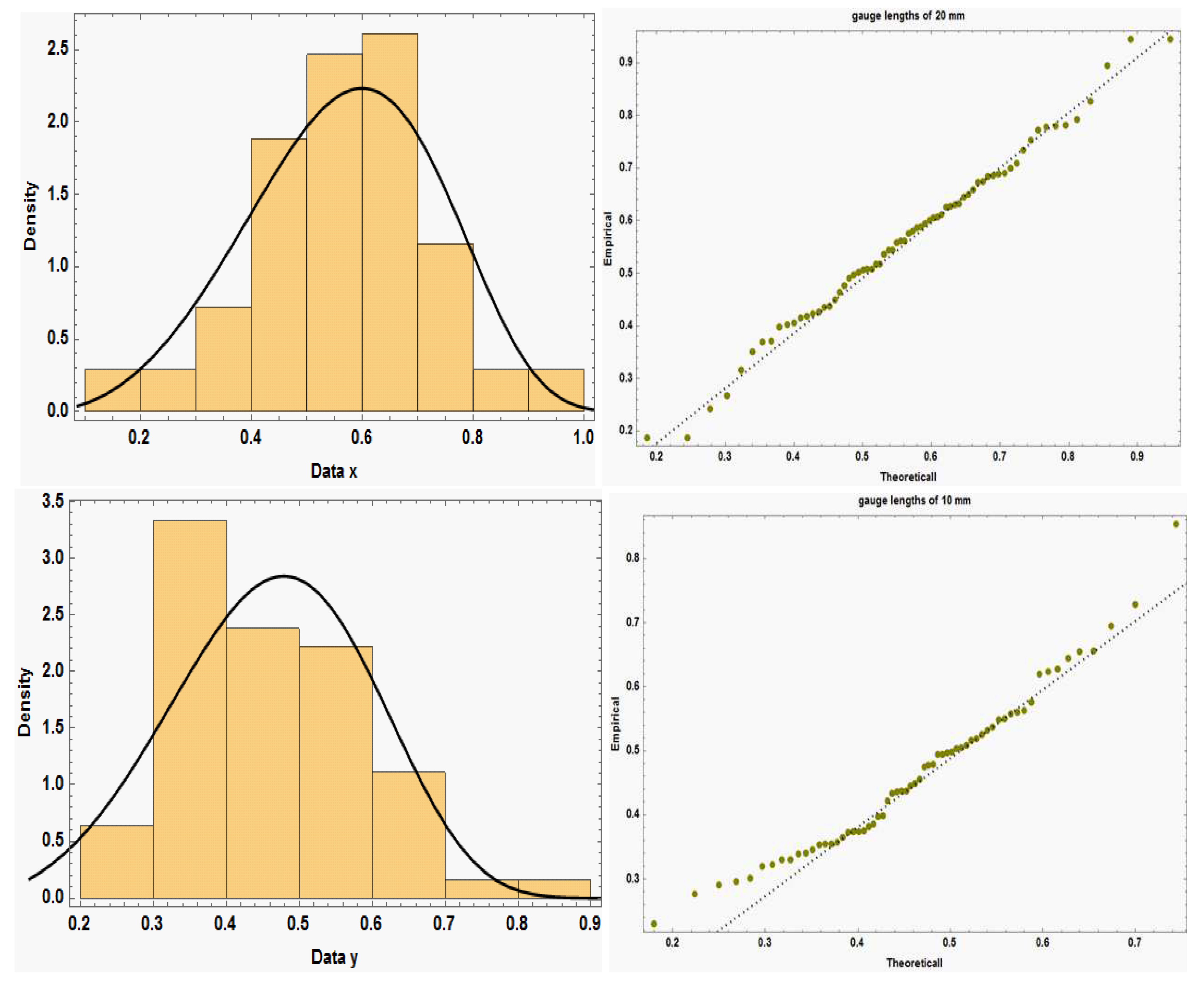
Figure 3. The fitted distribution functions for data sets 1 and 2 as well as the empirical distribution functions.

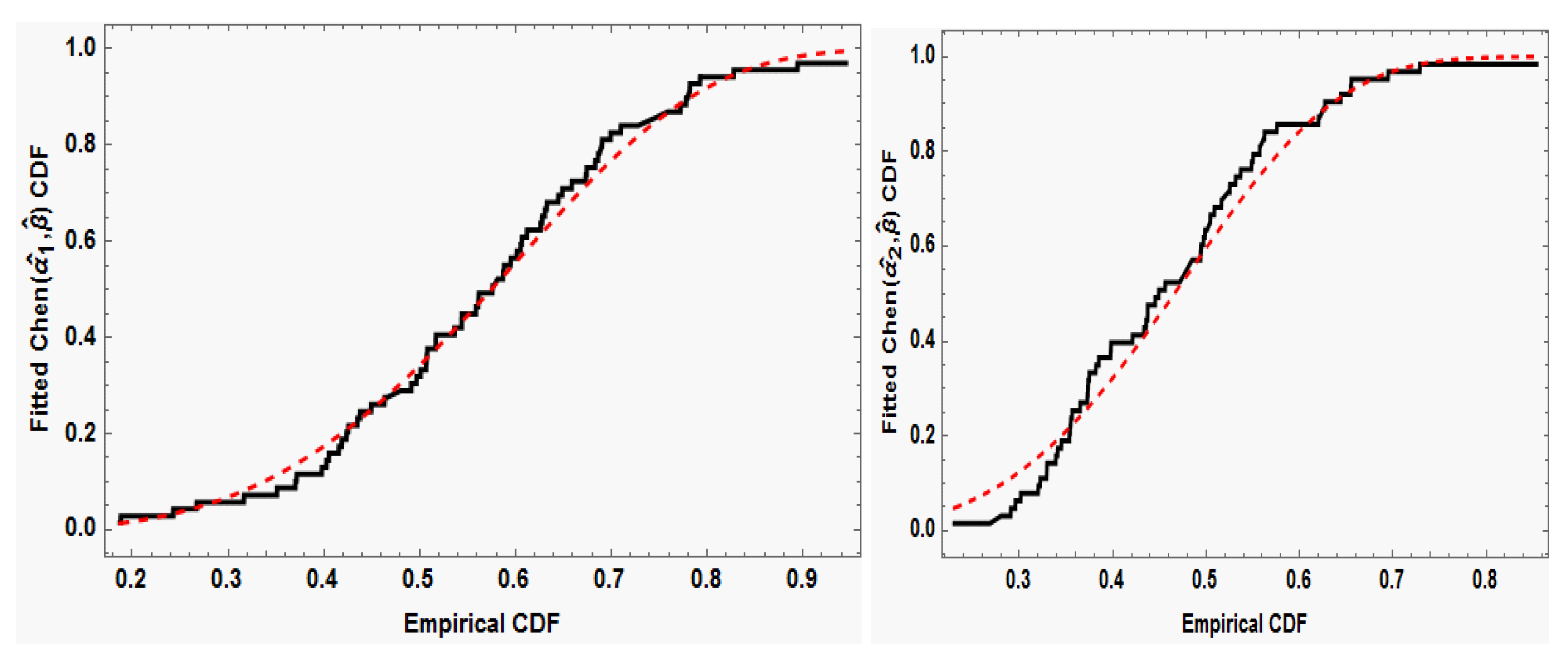
Table 3. The generated adaptive type-II progressively censored samples for carbon fiber data.

Scheme	Generated data
I	Type-II censoring:
	$m_{1} = 35$ , $m_{2} = 33$ , $T_{1} = 1.0$ , $T_{2} = 1.0$ , $R = (0^{* 34}, 34)$ and $S = (0^{* 32}, 30)$
	x	0.1873, 0.1880, 0.2430, 0.2673, 0.3167, 0.4053, 0.4157, 0.4187, 0.4237, 0.4257, 0.4913, 0.4967,
		0.5010, 0.5067, 0.5073, 0.5440, 0.5587, 0.5613, 0.5617, 0.5760, 0.6053, 0.6067, 0.6120, 0.6263,
		0.6277, 0.6733, 0.6743, 0.6833, 0.6863, 0.6893,0.7723, 0.7780, 0.7800, 0.7820, 0.7927.
	y	0.2302, 0.2764, 0.2906, 0.2956, 0.3014, 0.3200, 0.3222, 0.3292, 0.3294, 0.3390, 0.3408, 0.3448,
		0.3536, 0.3544, 0.3550, 0.3564, 0.3650, 0.3728, 0.3732, 0.3736, 0.3748, 0.3818, 0.3850, 0.3976,
		0.3980, 0.4212, 0.4334, 0.4356, 0.4374, 0.4374,
II	Censoring from the start:
	$m_{1} = 35$ , $m_{2} = 33$ , $T_{1} = 1.0$ , $T_{2} = 1.0$ , $R = (34, 0^{* 34})$ and $S = (30, 0^{* 32}) .$
	x	0.1873, 0.1880, 0.3167, 0.3703, 0.3717, 0.4053, 0.4157, 0.4187, 0.4257, 0.4377, 0.4633, 0.5010,
		0.5067, 0.5073, 0.5080, 0.5170, 0.5440, 0.5440, 0.5587, 0.5613, 0.5617, 0.5760, 0.5880, 0.6053,
		0.6277, 0.6307, 0.6447, 0.6490, 0.6587, 0.6863, 0.6903, 0.7780, 0.7820, 0.7927, 0.9450.
	y	0.2302, 0.2956, 0.3200, 0.3222, 0.3294, 0.3544, 0.3550, 0.3748, 0.3818, 0.4212, 0.4334, 0.4356,
		0.4374, 0.4374, 0.4454, 0.4560, 0.4750, 0.4790, 0.4946, 0.4986, 0.5028, 0.5088, 0.5254, 0.5316,
		0.5370, 0.5486, 0.5502, 0.5756, 0.6204, 0.6272, 0.6442, 0.6548, 0.695.
III	Progressive type-II censoring:
	$m_{1} = 35$ , $m_{2} = 33$ , $T_{1} = 1.0$ , $T_{2} = 1.0$ , $R = (2^{* 17}, 0^{* 18})$ and $S = (2^{* 15}, 0^{* 18}) .$
	x	0.1873, 0.1880, 0.2430, 0.2673, 0.3167, 0.3510, 0.4027, 0.4053, 0.4157, 0.4377, 0.4493, 0.4633,
		0.4763, 0.5073, 0.5080, 0.5170, 0.5613, 0.5617, 0.5760, 0.5800, 0.5950, 0.6013, 0.6053, 0.6263,
		0.6733, 0.6743, 0.6893, 0.6903, 0.6993, 0.7100, 0.7347, 0.7723, 0.7780, 0.7800, 0.9450.
	y	0.2302, 0.2764, 0.2906, 0.2956, 0.3014, 0.3200, 0.3292, 0.3294, 0.3390, 0.3408, 0.3536, 0.3544,
		0.3650, 0.3736, 0.3748, 0.3850, 0.3976, 0.4454, 0.4492, 0.4560, 0.4778, 0.4986, 0.5164, 0.5192,
		0.5370, 0.5486, 0.5574, 0.6204, 0.6242, 0.6272, 0.6442, 0.6548, 0.7290.
IV	Adaptive type-II progressive censoring:
	$m_{1} = 35$ , $m_{2} = 33$ , $T_{1} = 0.6$ , $T_{2} = 0.5$ , $R = (2^{* 17}, 0^{* 18})$ and $S = (2^{* 15}, 0^{* 18})$
	x	0.1873, 0.1880, 0.2430, 0.2673, 0.3167, 0.3510, 0.3703, 0.3717, 0.3980, 0.4027, 0.4053, 0.4237,
		0.4257, 0.4350, 0.4633, 0.4967, 0.5010, 0.5073, 0.5080, 0.5613, 0.5760, 0.5870, 0.5880, 0.6013,
		0.6067, 0.6120, 0.6307, 0.6587, 0.6833, 0.7100, 0.7723, 0.7780, 0.7820, 0.8277, 0.9450
	y	0.2302, 0.2764, 0.2906, 0.2956, 0.3014, 0.3200, 0.3292, 0.3294, 0.3390, 0.3408, 0.3536, 0.3544,
		0.3650, 0.3736, 0.3748, 0.3850, 0.3976, 0.4454, 0.4492, 0.4560, 0.4778, 0.4986, 0.5164, 0.5192,
		0.5370, 0.5486, 0.5574, 0.6204, 0.6242, 0.6272, 0.6442, 0.6548, 0.7290.

Figure 4. Data set histogram with Q-Q graphs and an estimated model density.

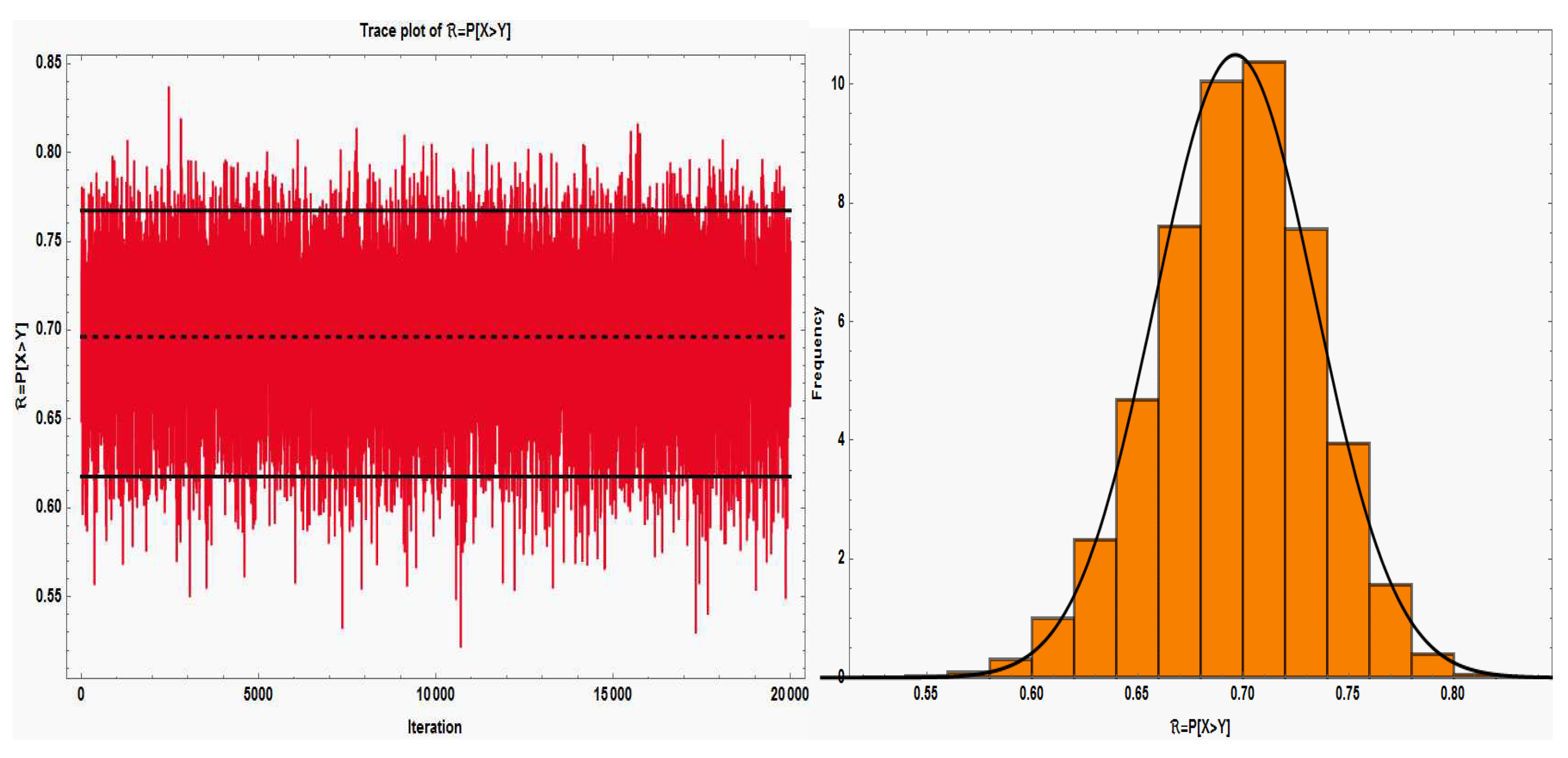
Table 4. ML, bootstrap and Bayes point estimates of ℜ for carbon fiber data.

Scheme	( $T_{1}, T_{2},$ , $J_{1},, J_{2})$	MLEs	Boot-p	BSE		BLINEX
				$ω$		$c = - 5$	$c = 0.5$	$c = + 5$
Complete data set	( $T_{1} = T_{2} = 1$ , $J_{1} = 96, J_{2} = 63$ )	0.6986	0.6992	0	0.6963	0.6999	0.6960	0.6927
				0.25	0.6969	0.6996	0.6966	0.6941
				0.50	0.6974	0.6992	0.6973	0.6956
				0.95	0.6985	0.6986	0.6984	0.6983
I	( $T_{1} = T_{2} = 1$ , $J_{1} = 35, J_{2} = 33$ )	0.8774	0.8817	0	0.8683	0.8716	0.8679	0.8647
				0.25	0.8706	0.8731	0.8703	0.8678
				0.50	0.8728	0.8745	0.8726	0.8709
				0.95	0.8769	0.8771	0.8769	0.8767
II	( $T_{1} = T_{2} = 1$ , $J_{1} = 35, J_{2} = 33$ )	0.6909	0.6907	0	0.6848	0.6922	0.6841	0.6770
				0.25	0.6864	0.6919	0.6858	0.6804
				0.50	0.6879	0.6916	0.6875	0.6838
				0.95	0.6906	0.6910	0.6906	0.6902
III	( $T_{1} = T_{2} = 1$ , $J_{1} = 35, J_{2} = 33$ )	0.6986	0.7000	0	0.6961	0.6997	0.6957	0.6924
				0.25	0.6967	0.6994	0.6964	0.6939
				0.50	0.6973	0.6991	0.6971	0.6954
				0.95	0.6984	0.6986	0.6984	0.6902
IV	( $T_{1} = 0.7, T_{2} = 0.5$ , $J_{1} = 23, J_{2} = 22$ )	0.6958	0.6947	0	0.6935	0.7006	0.6927	0.6861
				0.25	0.6941	0.6994	0.6935	0.6885
				0.50	0.6946	0.6982	0.6943	0.6909
				0.95	0.6957	0.6961	0.6957	0.6953

Table 5. Different interval estimates of ℜ for carbon fiber data.

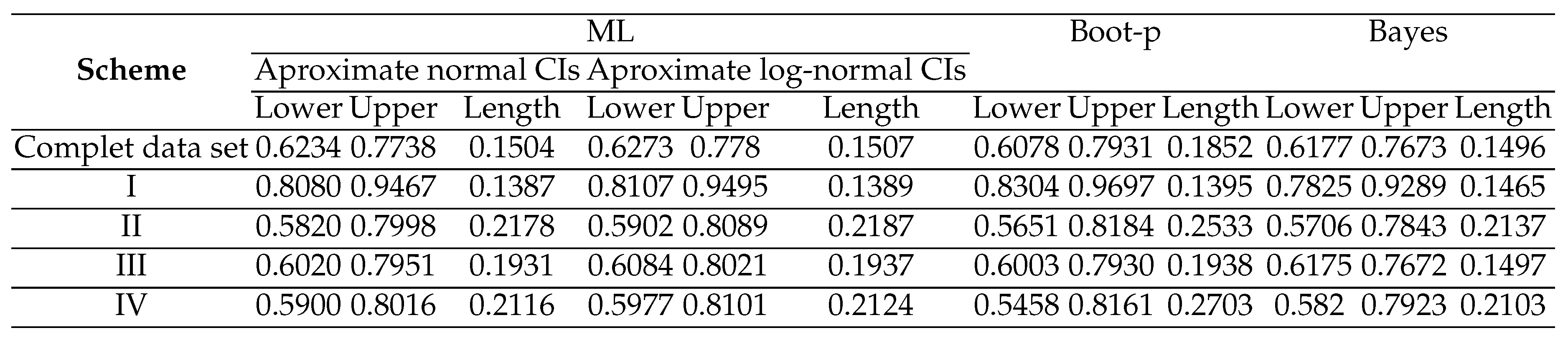
Analysis of an earlier real data set illustrates the significance and use of the adaptive type-II progressive censoring and the inferential methods based on it. It is demonstrated that the estimate of the S-S reliability model and the associated varied confidence intervals is highly dependent on the number of failures and a predefined number of inspection times. The performance of the various estimating techniques may also be observed to be rather similar to one another. Table 4’s numerical findings substantiate our understanding that, for ℜ, all Bayes estimation outcomes under the BSEL and BLINEX loss functions are equal to the respective MLEs as

ω

approaches unity. The results also show that the default estimators within the SE and LINEX loss functions, respectively, are derived from the default estimators based on both BSEL and BLINEX, when

ω = 0

. Thus, it is evident to us how important it is to use balanced loss functions in the Bayes approach. Table 5 indicates that the Bayes estimator is the best based on the length of the confidence interval. The estimators of approximate normal and approximate log-normal are next in order of preference, and the bootstrap estimator is the last one. Additionally, the values of the lengths of the confidence intervals based on the interval estimators of approximate normal and approximate log-normal exhibit a substantial convergence.

In summary, the results of point estimates and interval estimates do not change significantly between different schemes. It is evident that, as predicted in Tables 4 and 5, the estimates produced using the type-II censored data are nearer to the estimates produced with the complete sample. Although the adaptive type-II progressive censoring scheme shortens the testing time, the accuracy cannot be determined from a single sample so for better comparison we will create a simulation study in the next section.

5. Simulation and Comparisons

Numerous simulation tests are conducted to evaluate the accuracy of our estimations using Monte Carlo simulations. While the coverage percentage (CR) and interval mean length (IML) are used to evaluate interval estimation, the mean square error (MSE) and estimate value (VALUE) are used to evaluate point estimation. Smaller MSE and closer estimation value indicate better estimation performance for point estimation. Furthermore, in the context of interval estimation, better estimates are produced with greater coverage rates and shorter interval mean lengths.

First and foremost, the algorithm (Steps 2 and 3) provided in Subsection 2.2 must be used to construct adaptive type-II progressive censored data from an Chen distributions (

C h (α_{1}, β)

C h (α_{2}, β)

). It is established that the real values of (

α_{1}

α_{2}

β

) are (

1.5, 2.0, 0.75

). To facilitate comparison, we take into account

T_{1} = 0.6

T_{2} = 0.5

and (

N_{1}, m_{1}

) =(

N_{2}, m_{2}

(30, 10)

(30, 20)

(50, 10)

(50, 30)

, and

(50, 40)

. Three separate censoring schemes (CS) are selected for each combination of sample sizes and times

T_{1}

and

T_{2}

. We simplify the censoring schemes by abbreviating them. For instance, (

5^{* 2}, 0^{* 3}

) is the representation of (

5, 5, 0, 0, 0

). Every scenario involves 1000 iterations of the simulation. Mathematica software may then be used to do Monte Carlo simulations in order to obtain the corresponding MSEs and VALUEs for the point estimate and the related mean lengths and coverage rates for the interval estimation of ℜ. Based on these repeated samples, the following formulae are used to calculate the estimators’ bias, MSE, and lower bound:

Bias (\hat{ℜ}) = \frac{1}{1000} \sum_{i = 1}^{1000} |{\hat{ℜ}}_{(i)} - ℜ)|, and MSE (\hat{ℜ}) = \frac{1}{1000} \sum_{i = 1}^{1000} {({\hat{ℜ}}_{(i)} - ℜ)}^{2} .

The solutions of likelihood equations for the MLE are found by applying the Newton-Raphson technique. Additionally, we calculate the predicted length and coverage probability (CP) for the log- normal interval (Log-NCI), the percentile bootstrap interval (Boot-p), and the asymptotic confidence interval (ACI). We utilize 1000 bootstrap iterations to generate the bootstrap confidence intervals. It is configured with

γ = 0.05

as the significance threshold. Furthermore, two different prior types are taken into consideration to produce the Bayes estimates of ℜ: Prior 0 (

a_{i} = 0, b_{i} = 0, i = 1, 2, 3

) represents the non-informative prior scenario, whereas Prior 1 values (

a_{1} = 6, b_{1} = 4, a_{2} = 4, b_{2} = 2, a_{1} = 3, b_{1} = 4,

) represents the informative prior scenario, which are chosen such that the prior means match the original means. We have computed the Bayes estimates of ℜ under balanced (BSE, BLINEX) loss functions with different values of

ω

(

0, 0.25, 0.5, 0.95

) and LINEX constant c (

- 5, 5

). The Bayes estimates and corresponding credible credible intervals are calculated using

N = 11000

samples, and the first

M = 1000

values are discarded as the burn-in phase. The simulation results are reported in Tables 6 and 7. Based on the simulation results, we can conclude that:

According to the outcomes of our simulation, biases and MSEs are found to decrease with increasing sample sizes ( $N_{1}, N_{2}, m_{1}, m_{2}$ ).
Overall, none of the three censoring schemes performs better than the others when compared, although the random scheme (Scheme 3 in Table 6) performs better when it comes to minimal MSEs than the other two schemes. In most cases shown in Table 6, in terms of minimal MSEs, scheme 3, scheme 1, and scheme 2 are the schemes that perform the best through worst. This is true in several m and N cases.
The results indicate that the different estimations are successful since the estimated values are near to the actual values and the bias and mean square errors generally decrease as sample sizes ( $N_{1}, N_{2}, m_{1}, m_{2}$ ) grow.
The Bayes estimators seem to be sensitive to the assumed values of the prior parameters, based on the performance of the estimators based on Prior 0 and 1.
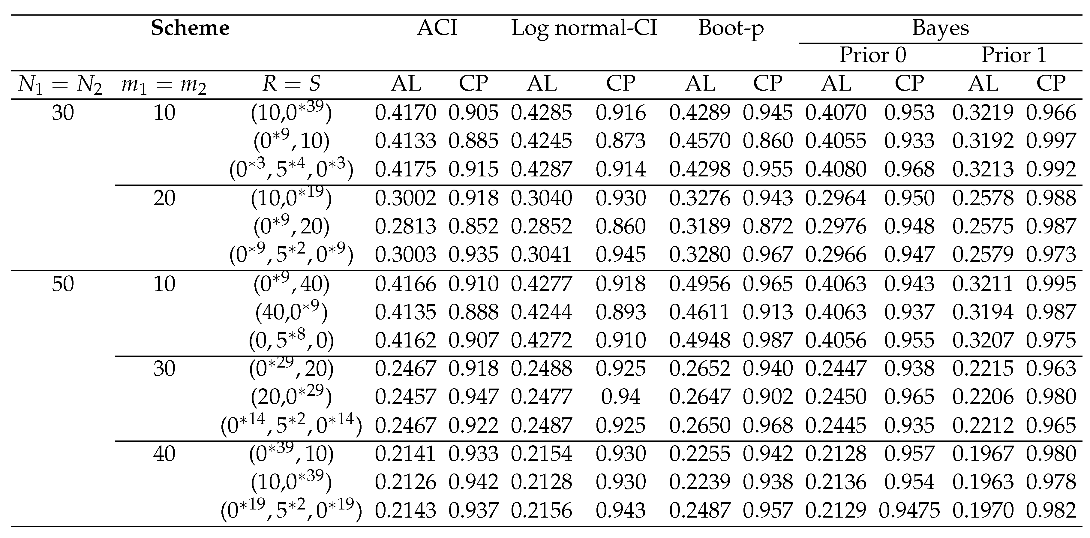
The Bayes estimate under LINEX with $ω = 0$ and $c = - 5$ provides better estimates for ℜ because of having the smallest MSEs.

The interval average lengths (ALs) and coverage probabilities (CPs) are used in Table 7 to compare the suggested confidence intervals. The following conclusions are drawn from these tables:
For various censoring schemes, in terms of interval length, the bootstrap interval is the largest, while the Bayesian credible intervals under both prior 0 and priors 1 are the smallest. Moreover, the asymptotic confidence intervals are the second-best ones.
By expanding the sample size, the average lengths (ALs) and the CPs for ML, bootstrap and Bayesian approaches have improved.
When comparing the confidence/credible interval lengths based on schemes 1 and 2 to those based on schemes 3, it is evident that the second scheme’s intervals in most cases for N and m have the shortest.
When the sample size increases, the coverage probabilities approach $1 - γ$ , indicating that the asymptotic confidence intervals will get more accurate. Through a comparison of the various credible and confidence intervals, it is clear that, in the majority of cases that are taken into consideration, the Bayes intervals offer the highest coverage percentages. Based on the Prior 1, the Bayes credible interval performs best. Further, in the case of traditional asymptotic intervals, the CPs are less than 0.95 and always more than 0.95 under Prior 1, but for Bayesian intervals they remain close to 0.95 under Prior 0. While the bootstrap confidence intervals is bigger than the other confidence intervals, it performs well in terms of coverage probability.

Table 6. Bias’s and MSE’s of the point estimations for ℜ when

T_{1} = 0.6, T_{2} = 0.5, ℜ = 0.5714 .

Table 6. Bias’s and MSE’s of the point estimations for ℜ when

T_{1} = 0.6, T_{2} = 0.5, ℜ = 0.5714 .

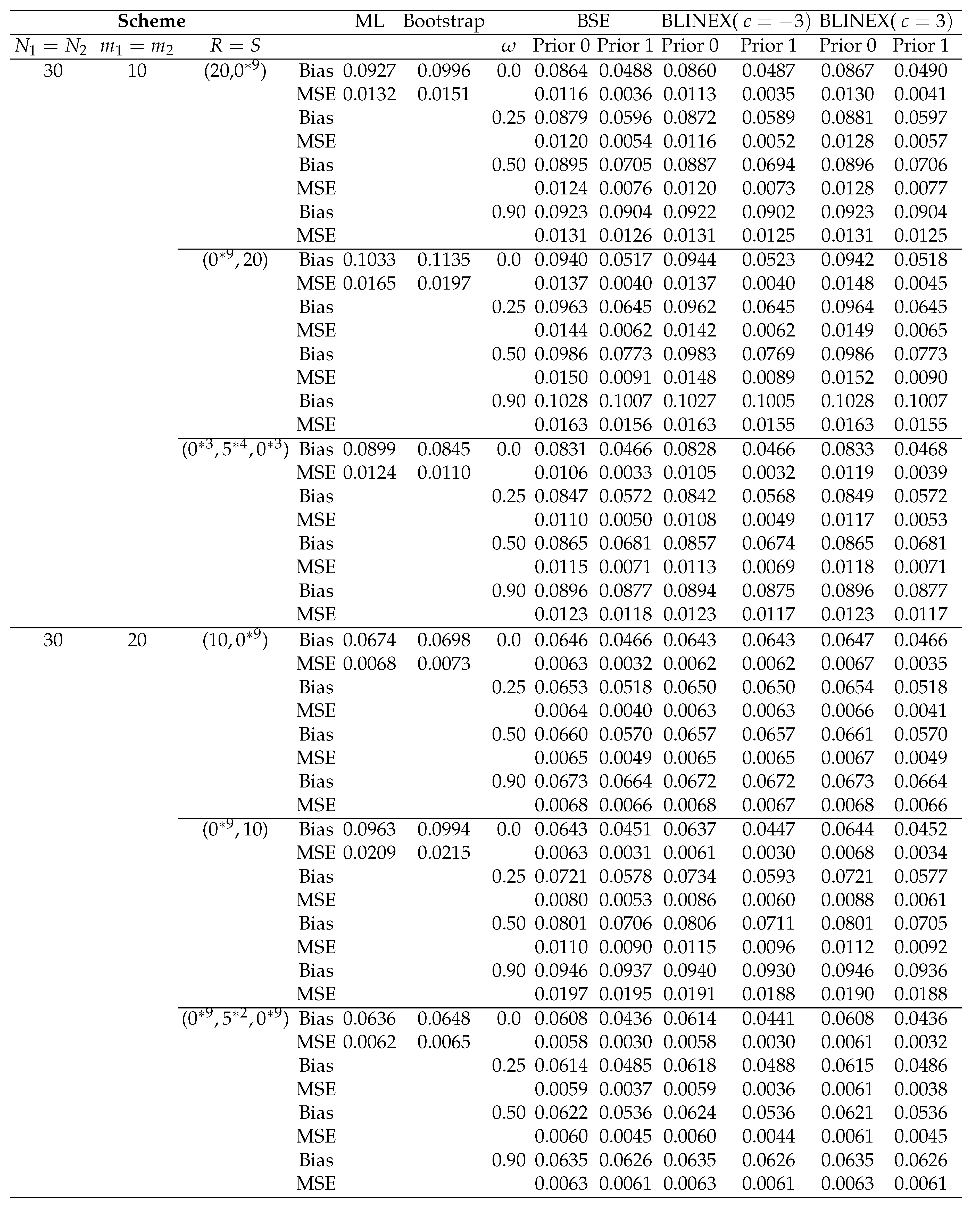
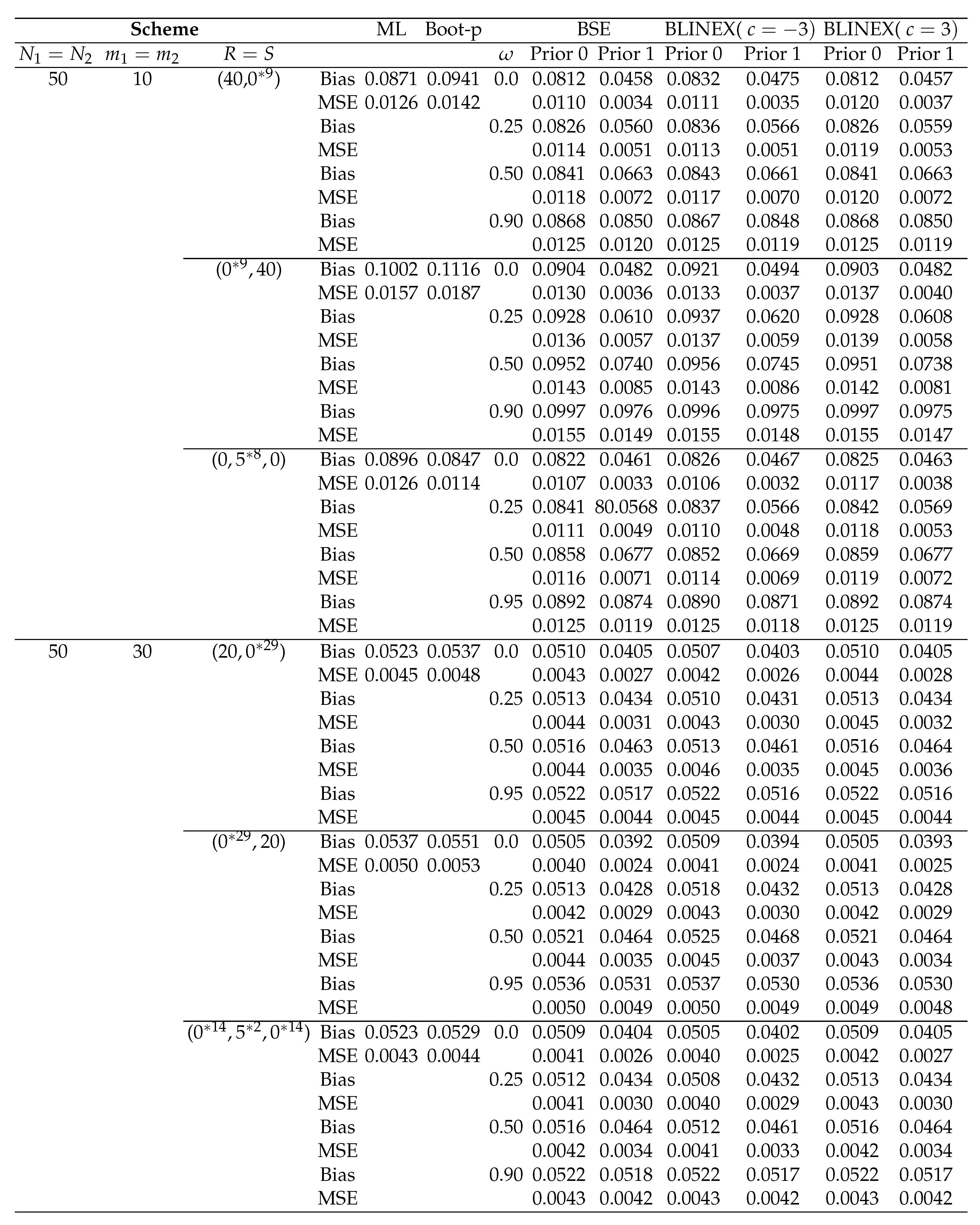
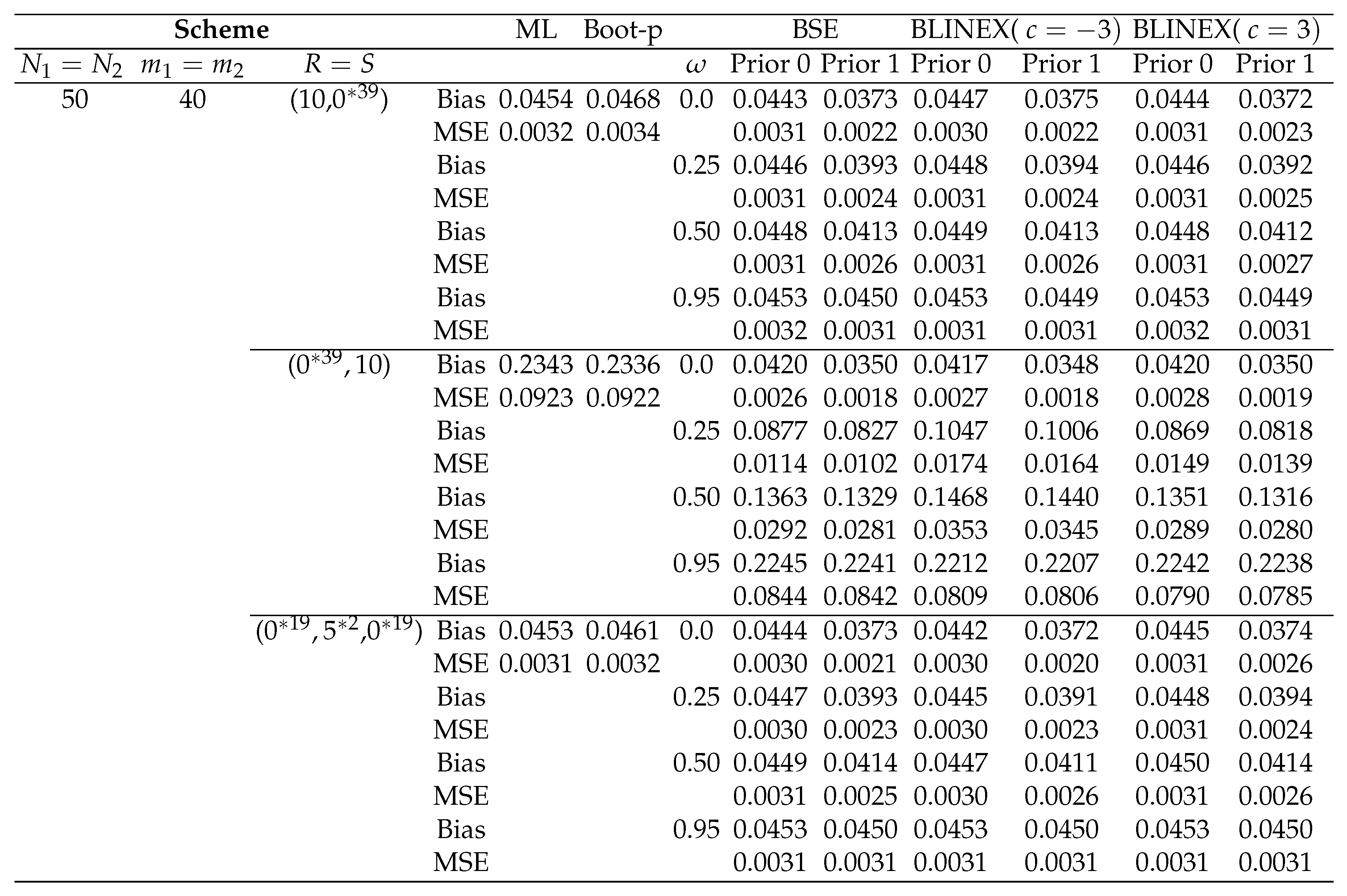
Table 7. Average confidence/credible interval lengths (AL) with for coverage percentage (CP)

T_{1} = 0.6, T_{2} = 0.5

Table 7. Average confidence/credible interval lengths (AL) with for coverage percentage (CP)

T_{1} = 0.6, T_{2} = 0.5

5.1. Conclusion

This study deals with the statistical inference of the stress-strength (S-S) reliability of Chen distribution under the assumption that the data are adaptive type-II progressively censored. The maximum likelihood approach is taken into consideration in order to determine the point as well as the interval estimates of the distribution’s S-S reliability. The parametric percentile bootstrap confidence interval and the approximated confidence intervals for the S-S reliability are derived. In order to obtain the approximate normal/log-normal intervals, the variance of the estimators of the S-S reliability is approximated using the delta method. We also revisit the gamma prior assumption-based Bayesian calculation of the stress-strength reliability. The Bayes estimates are derived by accounting for balanced squared error and balanced LINEX loss functions. We use the Markov chain Monte Carlo procedure to obtain the Bayes estimates and credible intervals for the highest posterior density. We compare the provided estimates in terms of their means squared error, confidence lengths, and coverage probabilities through an exhaustive numerical analysis. An application is examined to provide context for the recommended techniques. As can be seen from the numerical results, the Bayes estimates outperform estimates derived using the maximum likelihood approach. When utilising the asymmetric loss function in place of the symmetric loss, the Bayesian estimations yield more accurate estimates.

References

Agiwal, V. Bayesian estimation of stress strength reliability from inverse Chen distribution with application on failure time data. Annals of Data Science 2023, 10, 317–347. [CrossRef]
J. Ahmadi, M.J. Jozani, E. Marchand and A. Parsian, Bayes estimation based on k-record data from a general class of distributions under balanced type loss functions. Journal of Statistical Planning and Inference 2009, 139,1180–1189. [CrossRef]
E. A. Ahmed, Z. Ali Alhussain, M. M. Salah, H. Haj Ahmed, and M. S. Eliwa, Inference of progressively type-II censored competing risks data from Chen distribution with an application. Journal of Applied Statistics 2020, 47, 2492–2524. [CrossRef]
Almuqrin, M.A.; M. M.Salah, and E.A. Ahmed. Statistical Inference for Competing Risks Model with Adaptive Progressively Type-II Censored Gompertz Life Data Using Industrial and Medical Applications. Mathematics 2022, 10, 4274. [CrossRef]
A. Asgharzadeh, R. Valiollahi and M. Z. Raqab, Estimation of Pr(Y<X) for the two parameter generalized exponential records, Communications in Statistics-Simulation and Computation, 46 (2017), 371–394.
M. Bader, and A. Priest, Statistical Aspects of Fiber and Bundle Strength in Hybrid Composites. In: Hayashi, T., Kawata, S. and Umekawa, S., Eds., Progress in Science and Engineering Composites, ICCM-IV, Tokyo, (1982),1129-1136.
Z.W. Birnbaum and R.C. McCarty. A distribution-free upper confidence bound for Pr(Y<X), based on independent samples of x and y Ann. Math. Stat., 29 (1958), 558-562.
R. Calabria and G. Pulcini. Point estimation under asymmetric loss functions for left-truncated exponential samples. Commun. Statist. Theory Meth., 25:585–600,1996. [CrossRef]
G. Casella and E.I. George, Explaining the Gibbs sampler. Am Stat 46(1992),167–74.
Ç. Çetinkaya and A. I. Genç, Stress–strength reliability estimation under the standard two-sided power distribution. Applied Mathematical Modelling, 65 (2019), 72-88. [CrossRef]
Z. Chen, A new two-parameter lifetime distribution with bathtub shape or increasing failure rate function, Stat. Probab. Lett. 49(2000), 155–161. [CrossRef]
M. H. Chen, and Q. M. Shao, Monte Carlo estimation of Bayesian credible and HPD intervals. Journal of computational and Graphical Statistics, 8(1999), 69-92.
B. Efron and R. J. Tibshirani, An introduction to the bootstrap. CRC press, (1994).
W. H. Greene, Econometric Analysis, 4th Ed. New York: Prentice Hall, (2000).
M.E. Ghitany, D.K. Al-Mutairi and S.M Aboukhamseen, Estimation of the reliability of a stress-strength system from power Lindley distributions. Commun. Stat.-Simul. Comput. 44 (2015), 118–136. [CrossRef]
W.K. Hastings, Monte Carlo sampling methods using Markov chains and their applications. Biometrika 57(1970):97–109.
T. Kayal, Y. M. Tripathi, S. Dey, and S. J. Wu, On estimating the reliability in a multicomponent stress-strength model based on Chen distribution. Communications in Statistics-Theory and Methods, 49(2020), 2429-2447. [CrossRef]
T. Kayal, Y. M. Tripathi, D. P. Singh and M. K. Rastogi, Estimation and prediction for Chen distribution with bathtub shape under progressive censoring. Journal of Statistical Computation and Simulation, 87(2017), 348-366. [CrossRef]
S. Kotz, M. Lumelskii and M. Pensky, The stress-strength model and its generalizations: theory and applications, World Scientific, New-York, (2003).
D. Kundu, and R.D. Gupta, Estimation ofp(y < x) for weibull distributions. IEEE Trans. Reliability, 55(2006), 270-280.
B.X. Wang, Geng, Y.and J.X Zhou, Inference for the generalized exponential stress-strength model. Appl. Math. Model, 53 (2018), 267–275.
J. G. Ma, L. Wang, Y. M. Tripathi and M. K. Rastogi, Reliability inference for stress-strength model based on inverted exponential Rayleigh distribution under progressive Type-II censored data, Communications in Statistics-Simulation and Computation, 52 (2023), 2388-2407. [CrossRef]
N. Metropolis, A.W. Rosenbluth, M.N, Rosenbluth, A.H. Teller, E. Teller, Equation of state calculations by fast computing machines. J Chem Phys 21(1953),1087–92. [CrossRef]
H.K.T. Ng, D. Kundu, P.S. Chan, Statistical analysis of exponential lifetimes under an adaptive Type-II progressive censoring scheme. Naval Research Logistics (NRL). 2009; 56(8):687–698. [CrossRef]
M. Z. Raqab, O. M. Bdair and F. M. Al-Aboud, Inference for the two-parameter bathtub-shaped distribution based on record data. Metrika, 81, 229-253. [CrossRef]
M. K. Rastogi, Y. M. Tripathi and S.J. Wu, Estimating the parameters of a bathtub-shaped distribution under progressive type-II censoring, J. Appl. Statist. 39(2018), 2389–2411. [CrossRef]
C.P. Robert and G. Casella, Monte Carlo statistical methods. Springer, New York, (2004). [CrossRef]
A. M. Sarhan, and H. T. Ahlam, Stress-Strength Reliability Under Partially Accelerated Life Testing Using Weibull Model. Scientific African (2023): e01733.
A. M. Sarhan, B. Smith, D.C. Hamilton, Estimation of P(Y < X) for a two-parameter bathtub shaped failure rate distribution. Int J Stat Probab 4(2015 ),33–45. [CrossRef]
S. Shoaee and E. Khorram, Stress-strength reliability of a two-parameter bathtub-shaped lifetime distribution based on progressively censored samples. Communications in Statistics-Theory and Methods, 44(2015), 5306-5328. [CrossRef]
B. Tarvirdizade and M. Ahmadpour, Estimation of the stress–strength reliability for the two-parameter bathtub-shaped lifetime distribution based on upper record values. Statistical Methodology, 31(2016), 58-72. [CrossRef]
H.R. Varian, A Bayesian Approach to Real Estate Assessment, North-Holland, Amsterdam, (1975), 195-208.
F.K. Wang, A new model with bathtub-shaped failure rate using an additive Burr XII distribution, Reliab. Eng. System Safety. 70(2000), 305–312. [CrossRef]
L.Wang, K. Wu, Y. M. Tripathi and C. & Lodhi, Reliability analysis of multicomponent stress–strength reliability from a bathtub-shaped distribution. Journal of Applied Statistics, 49(2022), 122-142.
S. J. Wu, Estimation of the two-parameter bathtub-shaped lifetime distribution with progressive censoring. Journal of Applied Statistics, 35(2008), 1139-1150. [CrossRef]
M. Xie and C. D. Lai, Reliability analysis using an additive Weibull model with bathtub-shaped failure rate function, Reliability Engineeering and Systems Safety, 52(1995), 87-93. [CrossRef]
M. Xie, Y. Tang, and T.N. Goh, A modified Weibull extension with bathtub-shaped failure rate function, Reliab. Eng. System Safety. 76(2002), 279–285. [CrossRef]

Figure 1. Illustration of an adaptive type-II progressive censoring scheme.

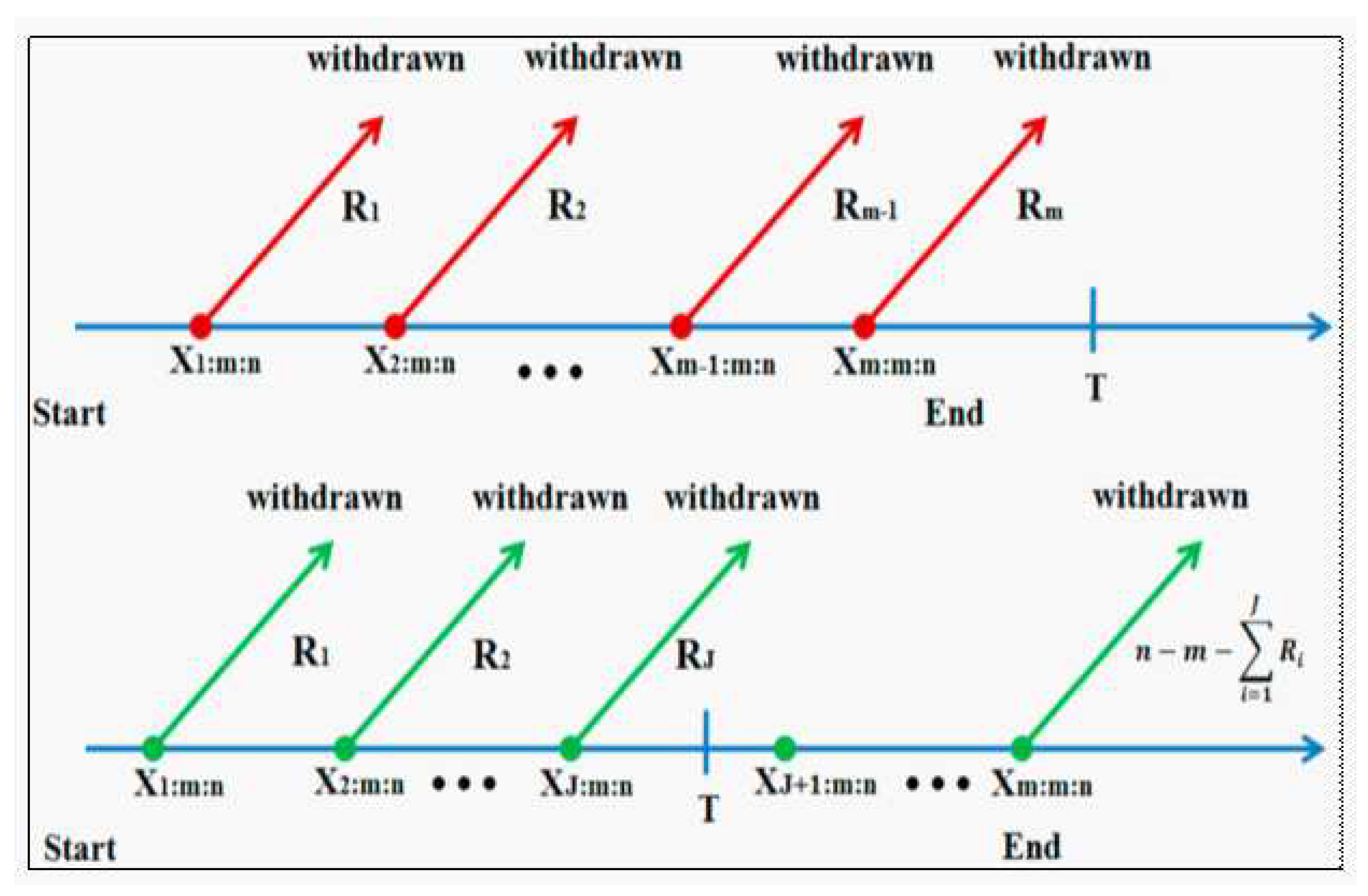
Table 1. Transformed Data Set I (for gauge lengths of 20 mm) from Çetinkaya and Genç (2019).

0.1873	0.4053	0.4913	0.5440	0.6053	0.6733	0.7723	0.1880	0.4157	0.4967	0.5587
0.6067	0.6743	0.7780	0.2430	0.4187	0.5010	0.5613	0.6120	0.6833	0.7800	0.2673
0.4237	0.5067	0.5617	0.6263	0.6863	0.7820	0.3167	0.4257	0.5073	0.5760	0.6277
0.6893	0.7927	0.3510	0.4350	0.5080	0.5800	0.6307	0.6903	0.8277	0.3703	0.4377
0.5170	0.5870	0.6327	0.6993	0.8943	0.3717	0.4493	0.5170	0.5880	0.6447	0.7100
0.9450	0.3980	0.4633	0.5363	0.5950	0.6490	0.7347	0.9450	0.4027	0.4763	0.5440
0.6013	0.6587	0.7540

Table 2. Transformed Data Set II (for gauge lengths of 10 mm) from Çetinkaya and Genç (2019).

0.2302	0.3408	0.3748	0.4454	0.5028	0.5574	0.6950	0.2764	0.3448	0.3818	0.4492
0.5044	0.5608	0.7290	0.2906	0.3536	0.3850	0.4560	0.5088	0.5624	0.8540	0.2956
0.3544	0.3976	0.4750	0.5164	0.5756	0.3014	0.3550	0.3980	0.4778	0.5192	0.6204
0.3200	0.3564	0.4212	0.4790	0.5254	0.6242	0.3222	0.3650	0.4334	0.4940	0.5316
0.6272	0.3292	0.3728	0.4356	0.4946	0.5370	0.6442	0.3294	0.3732	0.4374	0.4970
0.5486	0.6548	0.3390	0.3736	0.4374	0.4986	0.5502	0.6554

Disclaimer/Publisher’s Note: The statements, opinions and data contained in all publications are solely those of the individual author(s) and contributor(s) and not of MDPI and/or the editor(s). MDPI and/or the editor(s) disclaim responsibility for any injury to people or property resulting from any ideas, methods, instructions or products referred to in the content.

© 2023 by the authors. Licensee MDPI, Basel, Switzerland. This article is an open access article distributed under the terms and conditions of the Creative Commons Attribution (CC BY) license (http://creativecommons.org/licenses/by/4.0/).

Copyright: This open access article is published under a Creative Commons CC BY 4.0 license, which permit the free download, distribution, and reuse, provided that the author and preprint are cited in any reuse.

MDPI Initiatives

Important Links

Choose an area of interest and we will send you notifications of new preprints at your preferred frequency.

Disclaimer

Inference of Stress-Strength Reliability Based on Adaptive Progressive Type-II Censing from Bath Tube Distribution with Application to Carbon Fiber Data

Abstract

1. Introduction

2. Maximum Likelihood Estimation of ℜ

2.1. Asymptotic Confidence Interval of ℜ

2.2. Bootstrap Confidence Interval of ℜ

3. Bayes Estimation of ℜ

3.1. Prior and Posterior Distributions

3.2. Balanced Loss Function

3.3. Bayes Estimation Via MCMC Approach

4. Carbon Fiber Data Application

5. Simulation and Comparisons

5.1. Conclusion

References

MDPI Initiatives

Important Links

Subscribe