Generalized Bayes Prediction Study Based on Jointly Type-II Censored Sample from K-Exponential Populations

1. Introduction and motivations

Generalized Bayes is a Bayesian study based on a learning rate parameter ($\eta >0$) as a power of the likelihood function. The traditional Bayes framework is obtained for $\eta =1$, and we demonstrate the effect of the learning rate parameter on the prediction results. That is, if the prior distribution of the parameter $\theta$ is $\pi (\theta )$ then the generalized Bayes posterior distribution for $\theta$ is

$${\pi }^{\mathrm{*}}\left(\theta \right| data)\propto L^{\eta }\left(\theta ;data\right) \pi (\theta ), \theta \in \mathsf{\Theta }, \eta >0.$$

(1)

For more details on the generalized Bayes method and the choice of the value of the rate parameter we refer readers to [1-11]. An exact inference method based on maximum likelihood estimates (MLEs) was developed in [12], and its performance was compared with that of approximate, Bayesian, and bootstrap methods. The joint progressive censoring type II and the expected number of failures for two populations under the joint progressive censoring type II were introduced and studied by [13]. In contrast, exact likelihood inference for two exponential populations under joint progressive censoring of type II was studied in [14] and some precise results were obtained based on the maximum likelihood estimates developed by [15]. Exact likelihood inference for two populations of two-parameter exponential distributions under type II joint censoring was studied by [16].

One might be interested in predicting future failures using a joint type II censored sample. To accomplish this, prediction points or intervals should be determined. Bayesian prediction bounds for future observations based on certain distributions have been discussed by several authors. A study of Bayesian estimation and prediction based on a joint censored sample of type II from two exponential populations was presented by [17]. Prediction (various classical and Bayesian point predictors) for future failures in the Weibull distribution under hybrid censoring was studied by [18]. A Bayesian prediction based on generalized order statistics with multiple censoring of type II was developed by [19].

The main objective of this study is to predict future failures based on a joint type-II censoring scheme for k-exponential populations when censoring is performed on k-samples in a combined manner. Suppose that products from $k$ different lines are produced in the same factory, and $k$ independent samples of size $n_h,1\le h\le k$ are selected from these $k$ lines and simultaneously placed in a lifetime experiment. To reduce the cost and time of the experiment, the experimenter may decide to stop the lifetime test when a certain number ($r$) of failures occurs. The nature of the problem and the distributions used in our study are presented below.

Suppose $\{{\mathbf{X}}_h^{n_h},h=1,...,k\}$ are $k$-samples, where ${\mathbf{X}}_h^{n_h}=\{X_{h1},X_{h2},...,X_{h{n}_h}\}$ are the lifetimes of $n_h$ samples of product line $A_h$ and are assumed to be independent and identically distributed (iid) random variables from a population with a a probability density function (pdf) $f_h(x)$ and a cumulative distribution function (cdf) $F_h(x)$.

Furthermore, let $N={\sum }_{i=1}^k\mathrm{‍}{n}_i$ be the total sample size and let $r$ be the total number of observed failures. Let $W_1\le ...\le W_N$ denotes the order statistics of N random variables, $\{{\mathbf{X}}_h^{n_h},h=1,...,k\}$. Under the joint type- II censoring scheme for the $k$-samples, the observable data then consist of $(\mathsf{\delta },\mathbf{W})$, where $\mathbf{W}=(W_1,...,W_r), W_i\in \{{\mathbf{X}}_{h_i}^{{n_h}_i},h_i=1,...,k\}$, with $r<N$ being a pre-fixed integer and $\mathsf{\delta }=({\delta }_1(h),...,{\delta }_r(h))$ associated to $(h_1,...,h_r)$ is defined by

$${\delta }_i(h)=\left\{\begin{array}{ll}1,& \mathrm{i}\mathrm{f} h=h_i\\ 0,& \mathrm{o}\mathrm{t}\mathrm{h}\mathrm{e}\mathrm{r}\mathrm{w}\mathrm{i}\mathrm{s}\mathrm{e}.\end{array}\right.$$

(2)

Letting $M_r(h)={\sum }_{i=1}^r\mathrm{‍}{\delta }_i(h)$ denote the number of $X_h$-failures in $\mathbf{W}$ and $r={\sum }_{h=1}^k\mathrm{‍}{M}_r(h)$, then the joint density function of $(\mathsf{\delta },\mathbf{w})$ is given by

$$f(\mathsf{\delta },\mathbf{w})={\prod }_{h=1}^k\mathrm{‍}{c}_r({\overline{F}}_h(w_r){)}^{n_h-M_r(h)}.{\prod }_{i=1}^r\mathrm{‍}{\prod }_{h=1}^k\mathrm{‍}(f_h(w_i){)}^{{\delta }_i(h)}.$$

(3)

where ${\overline{F}}_h=1-F_h$, is the survival functions of $h^{th}$ population and $c_r=\frac{n_h!}{(n_h-M_r(h))!}$.

The joint density function of $(\mathsf{\delta },{\delta }_s,\mathbf{w},w_s),r<s\le N$ is given by

$$\begin{gathered} f(\mathsf{\delta },{\delta }_s,\mathbf{w},w_s)=\sum _{Q_{s-1}}\mathrm{‍}{\prod }_{h=1}^k\mathrm{‍}{c}_{1h}\{{\overline{F}}_h(w_r)- \\ {\overline{F}}_h(w_s){\}}^{M_{rs}(h)}({\overline{F}}_h(w_s){)}^{{\overline{n}}_{hs}}(f_h(w_s){)}^{{\delta }_s(h)} \end{gathered}$$

$$\times {\prod }_{i=1}^r\mathrm{‍}{\prod }_{h=1}^k\mathrm{‍}(f_h(w_i){)}^{{\delta }_i(h)}$$

(4)

where,

$w_r<w_s\le w_N, M_{rs}\left(h\right)=M_{s-1}\left(h\right)-M_r\left(h\right),{\overline{n}}_{hs}=n_h-M_s\left(h\right),c_{1h}=\frac{n_h!}{M_{rs}\left(h\right)!{\overline{n}}_{hs}!},$ ${\sum }_{{\mathbf{Q}}_{\mathbf{s}}}\mathrm{‍}={\sum }_{{\delta }_{r+1}=0}^1\mathrm{‍}...{\sum }_{{\delta }_s=0}^1\mathrm{‍}$ with $Q_s=\{\mathsf{\delta }\left(\mathbf{h}\right)=\left({\delta }_{r+1},...,{\delta }_s\right), \mathrm{f}\mathrm{o}\mathrm{r} 1\le h\le k\}$.

The conditional density function of $W_s$ given $(\mathsf{\delta },\mathbf{W})$, is given by

$$\begin{gathered} f\left(w_s\right|\mathsf{\delta },\mathbf{w})=\sum _{Q_s}\mathrm{‍}{\prod }_{h=1}^k\mathrm{‍}{c}_h(f_h(w_s){)}^{{\delta }_s\left(h\right)}\{{\overline{F}}_h(w_r)- \\ {\overline{F}}_h(w_s){\}}^{M_{rs}(h)}\frac{({\overline{F}}_h(w_s){)}^{{\overline{n}}_{hs}}}{({\overline{F}}_h(w_r){)}^{{\overline{n}}_{hr}}} \end{gathered}$$

$$=\sum _{Q_s}\mathrm{‍}{\prod }_{h=1}^k\mathrm{‍}{c}_h(f_h(w_s){)}^{{\delta }_s(h)}{\sum }_{l_h=0}^{M_{rs}(h)}\mathrm{‍}{a}_{l_h}\frac{({\overline{F}}_h(w_s){)}^{{\overline{n}}_{hs}+l_h}}{({\overline{F}}_h(w_r){)}^{{\overline{n}}_{h(s-1)}+l_h}}$$

(5)

where,

$$c_h=\frac{{\overline{n}}_{hr}!}{M_{rs}(h)!{\overline{n}}_{hs}!}, a_{l_h}=(-1{)}^{l_h}\left(\begin{array}{l}{M}_{rs}(h)\\ { l}_h\end{array}\right).$$

When the $k$populations are exponential with pdf and cdf respectively,

$$f_h={\theta }_h\mathrm{e}\mathrm{x}\mathrm{p}\left(-{\theta }_{h}x\right), F_h=1-\mathrm{e}\mathrm{x}\mathrm{p}\left(-{\theta }_{h}x\right), x>0,{\theta }_h>0; 1\le h\le k.$$

(6)

Then the likelihood function in (3) becomes

$$f(\mathsf{\Theta },\mathsf{\delta },\mathbf{w})=\prod _{h=1}^k\mathrm{‍}{c}_r\{\mathrm{e}\mathrm{x}\mathrm{p}(-{\theta }_h{w}_r){\}}^{{\overline{n}}_{hr}}\prod _{i=1}^r\mathrm{‍}\prod _{h=1}^k\mathrm{‍}\{{\theta }_h\mathrm{e}\mathrm{x}\mathrm{p}(-{\theta }_h{w}_i){\}}^{{\delta }_i(h)}$$

$$={\prod }_{h=1}^k\mathrm{‍}{c}_r{\theta }_h^{M_r(h)}\mathrm{e}\mathrm{x}\mathrm{p}\left\{-{\theta }_h{u}_h\right\}$$

(7)

where, $\mathsf{\Theta }=({\theta }_1,...,{\theta }_k)$ and $u_h={\sum }_{i=1}^r\mathrm{‍}{w}_i{\delta }_i(h)+w_r{\overline{n}}_{hr}$.

Substituting (6) into (5), we obtain the conditional density function of $W_s$, given $(\mathsf{\delta },\mathbf{W})$

$$f\left(w_s\right|\mathsf{\delta },\mathbf{w})=\sum _{Q_s}\mathrm{‍}{\prod }_{h=1}^k\mathrm{‍}{\theta }_h^{{\delta }_s(h)}{\sum }_{l_h=0}^{M_{rs}(h)}\mathrm{‍}{C}_h\mathrm{e}\mathrm{x}\mathrm{p}\{-{\theta }_h{D}_h(w_s-w_r)\}$$

(8)

where, $C_h=c_h{a}_{l_h}$, $D_h={\overline{n}}_{h(s-1)}+l_h$ and ${\overline{n}}_{hs}+{\delta }_s(h)={\overline{n}}_{h(s-1)}$.

Some special cases of the conditional density function are described as follows:

Case 1:

Suppose that $k-1$ is the number of samples satisfy${ M}_r(h)=n_h$ and only one sample satisfies $M_r(q)<n_q$ for $h=1,...,k,h\ne q$ equivalently $W_r>max\{{\mathbf{X}}_h^{n_h},h=1,...,k;h\ne q\}$ but $W_r\in \{{\mathbf{X}}_q^{n_q}\}$; $w_N=x_{q{n}_q}$.

In Case 1, the conditional density function of $W_s$ given $(\mathsf{\delta },\mathbf{W})$ is given by

$$f_1\left(w_s\right|\mathsf{\delta },\mathbf{w})=\frac{{\overline{n}}_{qr}!}{({\overline{n}}_{qr}-s+r)!}{\sum }_{l_q=0}^{s-r-1}\mathrm{‍}{a}_{l_q}{\theta }_q\mathrm{e}\mathrm{x}\mathrm{p}\{-{\theta }_q{D}_q(w_s-w_r)\}$$

(9)

where, $a_{l_q}=(-1{)}^{l_q}\left(\begin{array}{l}s-r-1\\ { l}_q\end{array}\right)$, $D_q={\overline{n}}_{qr}-s+r+l_q+1$, $w_r<w_s\le x_{q{n}_q}$.

Case 2:

Suppose that $k-R$ is the number of samples satisfy $M_r(h_i)=n_{h_i}$ for $h_i=1,...,k;$ and $R<k$ is the number of samples satisfy $M_r(h_j)<n_{h_j}$ for $h_j=1,...,k;h_i\ne h_j$, equivalently $W_r>max\{{\mathbf{X}}_{h_i}^{n_{h_i}},h_i=1,...,k\}$ but $W_r\in \{{\mathbf{X}}_{h_j}^{n_{h_j}},h_j=1,...,k;h_i\ne h_j\}$.

Under case 2, let’s just consider the $R$ samples, where $q=1,...,R$, then the conditional density function of $W_s$ given $(\mathsf{\delta },\mathbf{W})$ is given by

$$f_2(w_s|\mathsf{\delta },\mathbf{w})=\sum _{{Q^{\mathrm{\text{'}}}}_s}\mathrm{‍}{\prod }_{q=1}^R\mathrm{‍}{\theta }_q^{{\delta }_s(q)}{\sum }_{l_q=0}^{M_{rs}(q)}\mathrm{‍}{C}_q\mathrm{e}\mathrm{x}\mathrm{p}\{-{\theta }_q{D}_q(w_s-w_r)\} \mathrm{(1.10)}$$

where, ${Q^{\mathrm{\text{'}}}}_s=\{\mathsf{\delta }(\mathbf{q})=({\delta }_{r+1},...,{\delta }_s) \mathrm{f}\mathrm{o}\mathrm{r} 1\le q\le R\},C_q=c_q{a}_{l_q}$,$D_q={\overline{n}}_{q(s-1)}+l_q$ and ${\overline{n}}_{qs}+{\delta }_s(q)={\overline{n}}_{q(s-1)}$.

The remainder of this article is organized as follows. Section 2 presents the generalized Bayesian and Bayesian prediction points and intervals using squared error, Linex, and general entropy loss functions in the point predictor. A numerical study of the results from Section 2 is presented in Section 3. Finally, we conclude the paper in Section 4.

2. Generalized Bayes prediction

In this section, we introduce the concept of generalized Bayesian prediction, which is an investigation of Bayesian prediction under the influence of a learning rate parameter $\eta >0$. To apply the concept of generalized Bayesian prediction to a prediction study, we give a brief description of generalized Bayesian prediction based on a learning rate parameter $\eta >0$. A scheme for predicting a sample based on joint censoring of type II samples from k exponential distributions is presented. The main goal is to obtain the point predictors and prediction intervals given at the end of this section.

2.1. Generalized Bayes 

The parameters $\mathsf{\Theta }$ are assumed to be unknown, we may consider the conjugate prior distributions of $\mathsf{\Theta }$ as independent gamma prior distributions, i.e. ${\theta }_h\sim Gam(a_h,b_h)$. Hence, the joint prior distribution of $\mathsf{\Theta }$ is given by

$$\pi (\mathsf{\Theta })={\prod }_{h=1}^k\mathrm{‍}{\pi }_h({\theta }_h),$$

(10)

where

$${\pi }_h({\theta }_h)=\frac{b_h^{a_h}}{\mathsf{\Gamma }(a_h)} {\theta }_h^{a_h-1}\mathrm{e}\mathrm{x}\mathrm{p}\{-b_h{\theta }_h\},$$

(11)

and $\mathsf{\Gamma }(\cdot )$ denotes the complete gamma function.

Combining (7) and (10) after raising (7) to the power $\eta$, the posterior joint density function of $\mathsf{\Theta }$ is then

$${\pi }^{\mathrm{*}}\left(\mathsf{\Theta }\right| data)=\prod _{h=1}^k\mathrm{‍}\frac{(u_h\eta +b_h{)}^{\eta M_r(h)+a_h}{\theta }_h^{\eta M_r(h)+a_h-1}}{\mathsf{\Gamma }(\eta M_r(h)+a_h)}\mathrm{e}\mathrm{x}\mathrm{p}\{-{\theta }_h(u_h\eta +b_h)\},$$

$$={\prod }_{h=1}^k\mathrm{‍}\frac{{\xi }_h^{{\mu }_h}{\theta }_h^{{\mu }_h-1}}{\mathsf{\Gamma }({\mu }_h)}\mathrm{e}\mathrm{x}\mathrm{p}\{-{\theta }_h{\xi }_h\},$$

(12)

where, ${\xi }_h=u_h\eta +b_h, {\mu }_h=\eta M_r(h)+a_h$.

Since ${\pi }_h$ is a conjugate prior, where ${\theta }_h\sim Gam(a_h,b_h)$ then it follows that the posterior density function of $({\theta }_h|data)$ is $Gam(\eta M_r(h)+a_h,u_h\eta +b_h)$.

2.2. One sample prediction 

A sample prediction scheme for the case of joint censoring of samples from two exponential distributions was studied in [17] and then three cases for the future failures were derived, where in the first case the future predicted failure surly belongs to ${\mathit{X}}_1^{n_1}$ failures if $M_r\left(1\right)<n_1,M_r\left(2\right)=n_2$, second case, the future predicted failure surly belongs to ${\mathit{X}}_2^{n_2}$ failures if $M_r\left(2\right)<n_2,M_r\left(1\right)=n_1$, third case, it is unknown to which sample the future predicted failure belongs. Here, we generalize the results reported in [17] and examine two special cases in addition to the general case.

In the general case, the size of any sample is greater than the number of observed failures; that is, $M_r\left(h\right)<n_h\equiv w_r<x_{h{n}_h}$ for $h=1,...,k.$ The first special case arises when all future values (predictors) belong to only one sample and the observations of the remaining $k-1$samples are less than $w_r$. The second special case arises when all future values (predictors) belong to some samples and all observations of the other samples are less than $w_r$. The forms of all functions related to the second special case are similar to those related to the general case; therefore, we will introduce only the general case and the first special case.

For the general case, to predict $w_r$ for $r<s\le N$ based on the observed data $(\mathsf{\delta },\mathbf{w})$, we use the conditional density function $(9)$. Let us define the following integral

$$I_h^{{\delta }_s(h)}=\frac{{\xi }_h^{{\mu }_h}}{\mathsf{\Gamma }({\mu }_h)}{\int }_0^{\infty }\mathrm{‍}{\theta }_h^{{\mu }_h-1+{\delta }_s(h)}\mathrm{e}\mathrm{x}\mathrm{p}\left\{-{\theta }_h\left[{\xi }_h+D_h({\omega }_s-{\omega }_r)\right]\right\}\mathrm{d}{\theta }_h$$

$$=\left\{\begin{array}{c}\frac{{\mu }_h}{{\xi }_h}{\left(1+\frac{D_h\left({\omega }_s-{\omega }_r\right)}{{\xi }_h}\right)}^{-\left({\mu }_h+1\right)}, for {\delta }_s\left(h\right)=1\\ {\left(1+\frac{D_h\left({\omega }_s-{\omega }_r\right)}{{\xi }_h}\right)}^{-{\mu }_h} , for {\delta }_s\left(h\right)=0\end{array}\right.$$

(13)

Using (8), (12), and (13) the Bayesian predictive density function of $w_s$, given $(\mathsf{\delta },\mathbf{w})$, is given by

$$\begin{gathered} f_B\left({\omega }_s |\mathsf{\delta },\mathbf{w}\right)={\int }_{\mathsf{\Theta }}\mathrm{‍}f\left(w_s|\mathsf{\delta },\mathrm{w}\right){\pi }^{\mathrm{*}}\left(\mathsf{\Theta }|\mathsf{\delta },\mathrm{w}\right)d\mathsf{\Theta } \\ =\sum _{Q_s}\mathrm{‍}{\prod }_{h=1}^k\mathrm{‍}{\sum }_{l_h=0}^{M_{rs}}\mathrm{‍}\frac{C_h{\xi }_h^{{\mu }_h}}{\mathsf{\Gamma }\left({\mu }_h\right)}{\int }_0^{\infty }\mathrm{‍}{\theta }_h^{{\mu }_h-1+{\delta }_s\left(h\right)}\mathrm{e}\mathrm{x}\mathrm{p}\left\{-{\theta }_h\left[{\xi }_h+D_h\left({\omega }_s-{\omega }_r\right)\right]\right\}\mathrm{d}{\theta }_h \\ ={\sum }_{Q_s}{\prod }_{h=1}^k{C}_h\left\{{\sum }_{\upsilon =1}^k\left(I_{\upsilon }^1 {\prod }_{q=1,q\ne \upsilon }^k{I}_q^0\right)\right\}, \end{gathered}$$

(14)

Where

$${\prod }_{h=1}^k\mathrm{‍}{\int }_0^{\infty }\mathrm{‍}f({\theta }_h)d{\theta }_h={\int }_0^{\infty }\mathrm{‍}...{\int }_0^{\infty }\mathrm{‍}f({\theta }_1)...f({\theta }_k)d{\theta }_1...d{\theta }_k.$$

Under case 1, the Bayesian predictive density function of $w_s$, given $(\mathsf{\delta },\mathrm{w})$, is given by

$$f_{1B}\left(w_s|\mathsf{\delta },\mathbf{w}\right)=\frac{{\overline{n}}_{qr}!{\mu }_q}{\left({\overline{n}}_{qr}-s+r\right)!{\xi }_q}{\sum }_{l_q=0}^{s-r-1}\mathrm{‍}{a}_{l_q}{\left(1+\frac{D_q(w_s-w_r)}{{\xi }_q}\right)}^{-({\mu }_q+1)},$$

(15)

where, ${\xi }_q=u_q\eta +b_q,{\mu }_q=\eta M_r(q)+a_q$, $w_r<w_s\le x_{q{n}_q}$.

2.3. Bayesian point predictors 

For the point predictor, we considered three types of loss functions:

(i). The squared error loss function (SE), which is classified as a symmetric function, is given by

$$L_{SE}({\phi }^{\mathrm{*}},\phi )\propto ({\phi }^{\mathrm{*}}-\phi {)}^2,$$

where ${\phi }^{\mathrm{*}}$ is an estimate of $\phi .$

(ii). The Linex loss function, which is asymmetric is given by

$$L_L\left({\phi }^{\mathrm{*}},\phi \right)\propto e^{\tau \left({\phi }^{\mathrm{*}}-\phi \right)}-\tau \left({\phi }^{\mathrm{*}}-\phi \right)-1, \tau \ne 0.$$

(iii). The generalization of the entropy (GE) loss function is

$$L_{GE}\left({\phi }^{\mathrm{*}},\phi \right)\propto {\left(\frac{{\phi }^{\mathrm{*}}}{\phi }\right)}^c-c\ln \left(\frac{{\phi }^{\mathrm{*}}}{\phi }\right)-1, c\ne 0.$$

It is worth noting that the Bayes estimates under the GE loss function coincide with those under the SE loss function when $c=-1.$ However, when $c=1,-2,$the Bayes estimates under GE become those under the weighted squared error loss function and the precautionary loss function, respectively.

Now, the Bayesian point predictors $W_s, r<s\le N$, under different loss functions (SE, Linex, GE) can be obtained using the predictive density function (14), which are denoted respectively by $W_{SP},W_{LP},W_{EP}$ and given as follows:

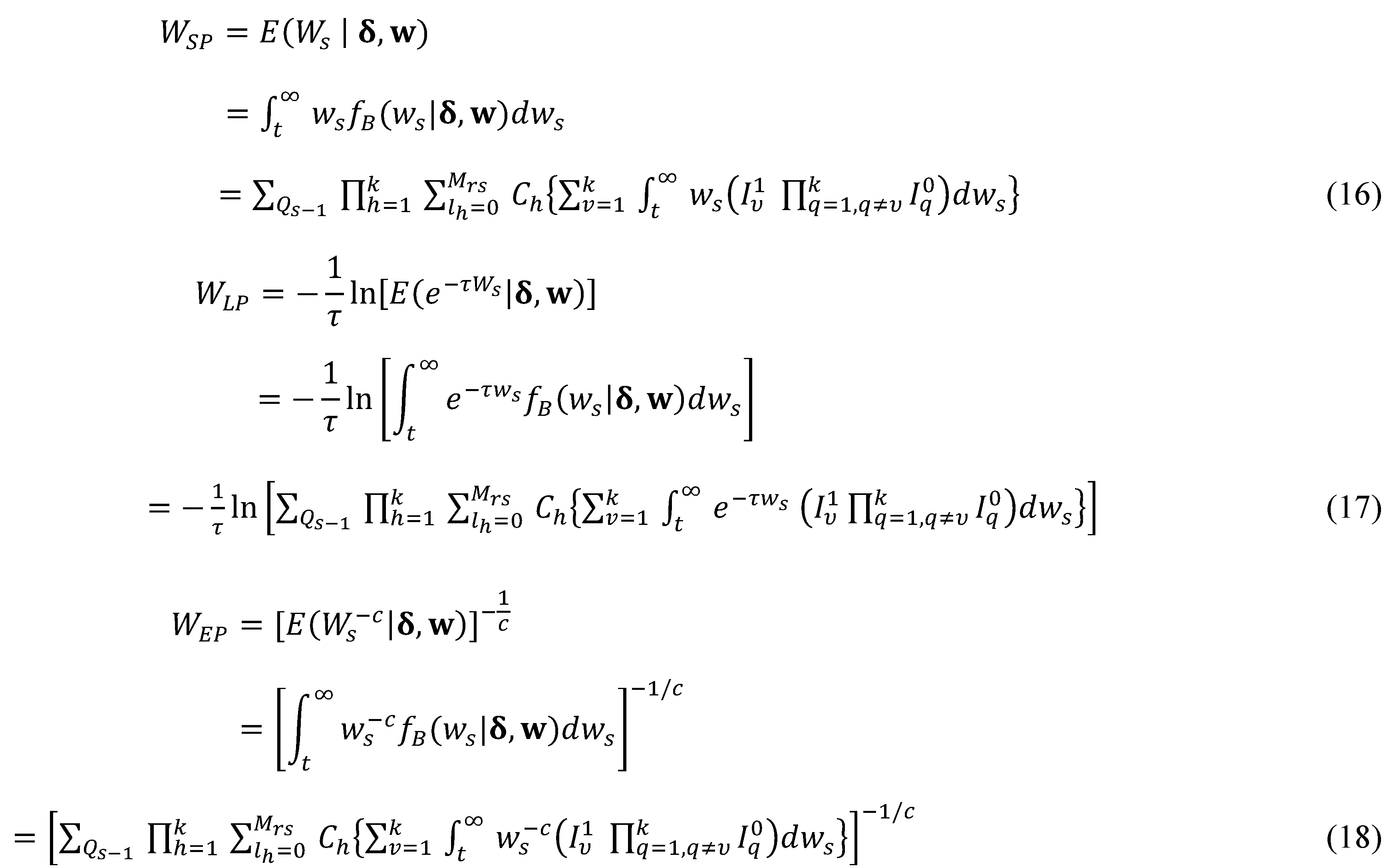
Under case 1, $W_{SP},W_{LP},W_{EP}$ are respectively given by

$$W_{SP}=\frac{{\overline{n}}_{qr}!{\mu }_q}{({\overline{n}}_{qr}-s+r)!{\xi }_q}{\sum }_{l_q=0}^{s-r-1}\mathrm{‍}{a}_{l_q}{\int }_t^{\infty }\mathrm{‍}{w}_s(1+\frac{D_q({\omega }_s-{\omega }_r)}{{\xi }_q}{)}^{-({\mu }_q+1)}d{\omega }_s$$

(19)

$$W_{LP}=-\frac{1}{\tau }\mathrm{l}\mathrm{n}\left[\frac{{\overline{n}}_{qr}!{\mu }_q}{({\overline{n}}_{qr}-s+r)!{\xi }_q}{\sum }_{l_q=0}^{s-r-1}\mathrm{‍}{a}_{l_q}{\int }_t^{\infty }\mathrm{‍}{e}^{-\tau w_s}(1+\frac{D_q({\omega }_s-{\omega }_r)}{{\xi }_q}{)}^{-({\mu }_q+1)}d{\omega }_s\right]$$

(20)

$$W_{EP}={\left[\frac{{\overline{n}}_{qr}!{\mu }_q}{({\overline{n}}_{qr}-s+r)!{\xi }_q}{\sum }_{l_q=0}^{s-r-1}\mathrm{‍}{a}_{l_q}{\int }_t^{\infty }\mathrm{‍}{w}_s^{-c}(1+\frac{D_q({\omega }_s-{\omega }_r)}{{\xi }_q}{)}^{-({\mu }_q+1)}d{\omega }_s\right]}^{-1/c}$$

(21)

Numerical integration is required to obtain the predictors $W_{SP},W_{LP},W_{EP}$.

2.4. Prediction Interval 

The predictive survival function of $W_s$ is given by

$$\begin{gathered} {\overline{F}}_B\left(t\right)=P\left(W_s>t |\mathsf{\delta },\mathbf{w}\right)={\int }_t^{\infty }\mathrm{‍}{f}_B\left(w_s|\mathsf{\delta },\mathrm{w}\right)d{w}_s \\ =\sum _{Q_{s-1}}\mathrm{‍}{\prod }_{h=1}^k\mathrm{‍}{\sum }_{l_h=0}^{M_{rs}}\mathrm{‍}{C}_h\left[{\sum }_{v=1}^k\mathrm{‍}{\int }_t^{\infty }\mathrm{‍}\left(I_{\upsilon }^1 {\prod }_{q=1,q\ne \upsilon }^k{I}_q^0\right)d{w}_s\right] \end{gathered}$$

(22)

Numerical integration is required to obtain the predictive distribution function in Equation (22). In Case 1, the predictive survival function of $W_s$ is given by

$${\overline{F}}_{1B}\left(t\right)=P\left(W_s>t|\mathsf{\delta },\mathrm{w}\right)={\int }_t^{\infty }\mathrm{‍}{f}_{1B}\left(w_s|\mathsf{\delta },\mathrm{w}\right)d{w}_s$$

$$=\frac{{\overline{n}}_{qr}!}{({\overline{n}}_{qr}-s+r)!}{\sum }_{l_q=0}^{s-r-1}\mathrm{‍}\frac{a_{l_q}}{D_q}{\left(1+\frac{D_q(t-w_r)}{{\xi }_q}\right)}^{-{\mu }_q}.$$

(23)

The Bayesian predictive bounds of a two-sided equi-tailed $100(1-\gamma )\mathrm{\%}$ interval for $W_s, r<s\le N$, can be obtained by solving the following two equations,

$$\overline{F}(L|\mathsf{\delta },\mathrm{w})=1-\frac{\gamma }{2}, \overline{F}(U|\mathsf{\delta },\mathrm{w})=\frac{\gamma }{2}$$

(24)

3. Numerical study

In this section, the results of the Monte Carlo simulation study are conducted to evaluate the performance of the prediction study derived in the previous section, and an example is presented to illustrate the prediction methods discussed here.

3.1. Simulation study 

We considered three samples from three populations with $(n_1,n_2,n_3,r)$ for choices $(10,10,10,25)$ and $(15,15,15,40)$. In case 1, we choose the exponential parameters $({\theta }_1,{\theta }_2,{\theta }_3)$ as (2, 1, 0.1) based on the hyperparameters represented by $\mathsf{\Delta }=(a_1,b_1,a_2,b_2,a_3,b_3)$, where $\mathsf{\Delta }={\mathsf{\Delta }}_1=(\mathrm{2,1},\mathrm{2,2},\mathrm{1,10})$.

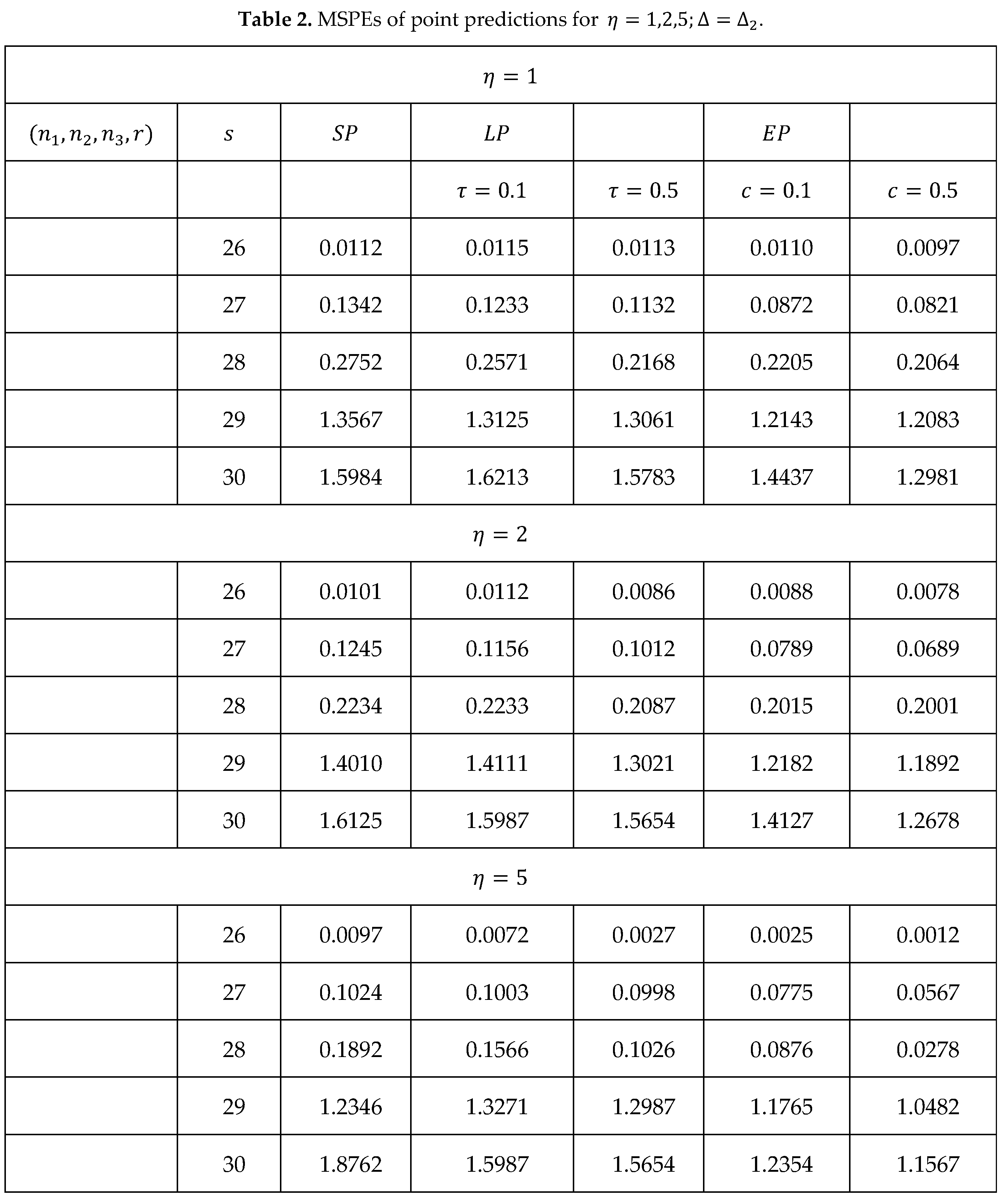
In the general case we choose the exponential parameters $({\theta }_1,{ \theta }_2,{\theta }_3)$ as (2, 2.5, 3 ) based on the hyperparameters $\mathsf{\Delta }={\mathsf{\Delta }}_2=(2,1,5,2,3,1)$.

For the generalized Bayesian study, three values are chosen for the learning rate parameter $\eta =1,2,5$ and 10,000 repetitions are used for the Monte Carlo simulations. For $(n_1,n_2,n_3,r)=(10,10,10,25)$, under case 1 we use (19), (20) and (21), to calculate the mean squared prediction errors (MSPEs) of the point predictors ($W_{SP},W_{LP},W_{EP}$) for $s=26,...,30$, where $\tau =\mathrm{0.1,0.5}$; $c=\mathrm{0.1,0.5}$ and the results are presented in Table 1.

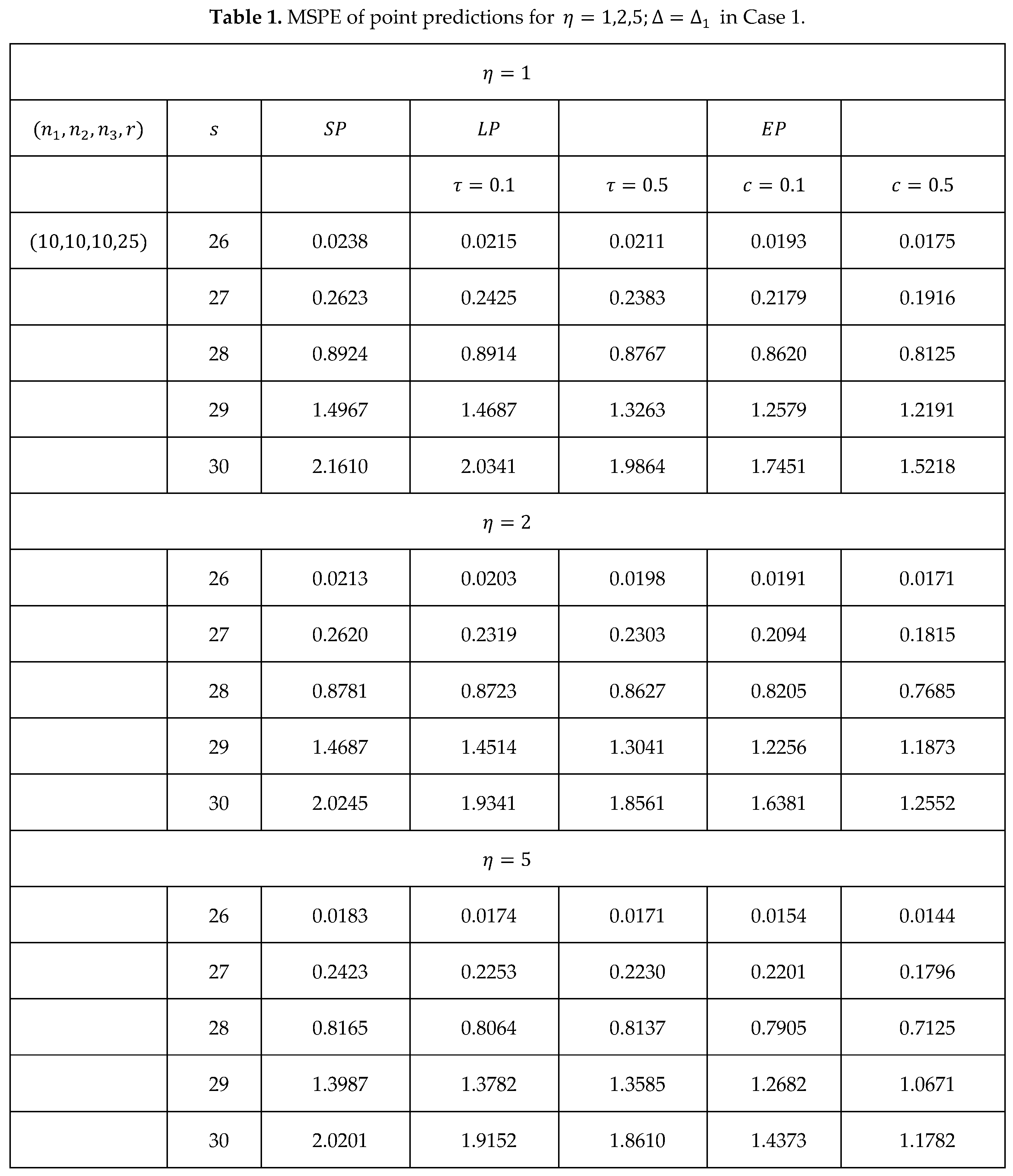
The results of the MSPEs in the general case are calculated using (16), (17), and (18) and shown in Table 2.

For $(n_1,n_2,n_3,r)=(10,10,10,25)$ and $(n_1,n_2,n_3,r)=(\mathrm{15,15,15,40})$ the results of the prediction bounds of $W_s, s=26,...,30$ and $s=41,...,45$, respectively are calculated using (23), (24) in Case 1 then are presented in Table 3.

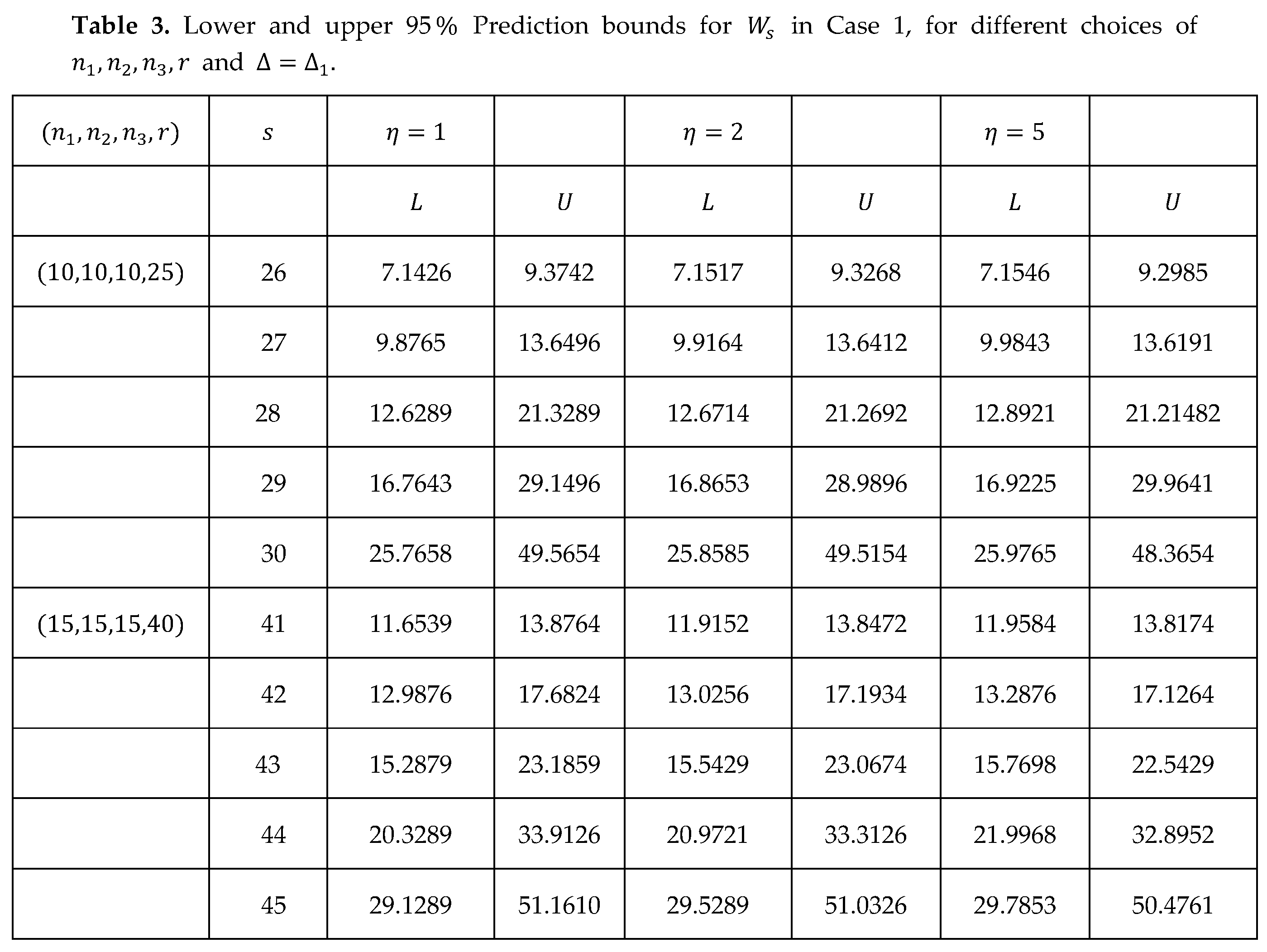
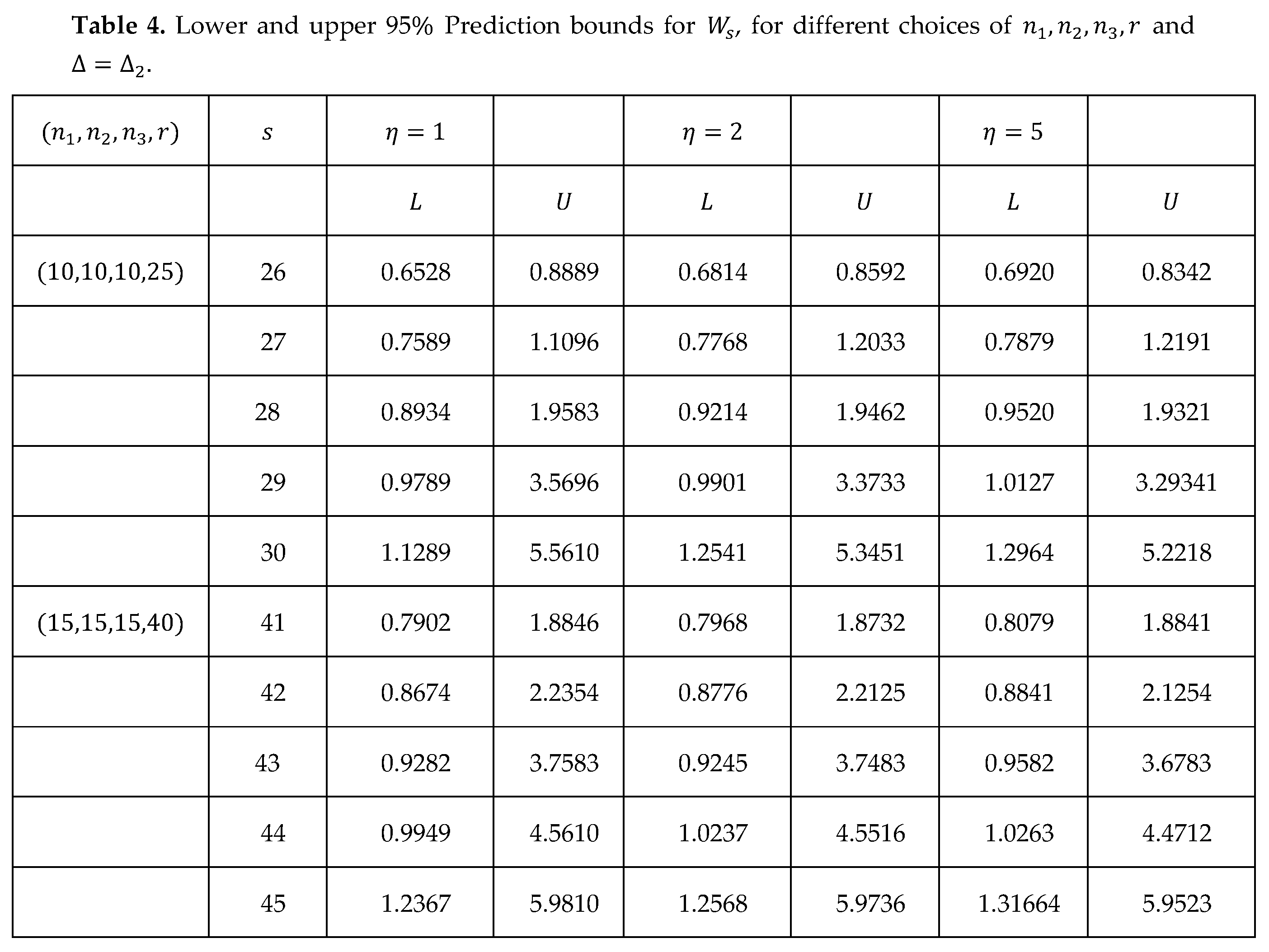
Table 4 presents the prediction bounds using (22), (24) to show the results of the general case.

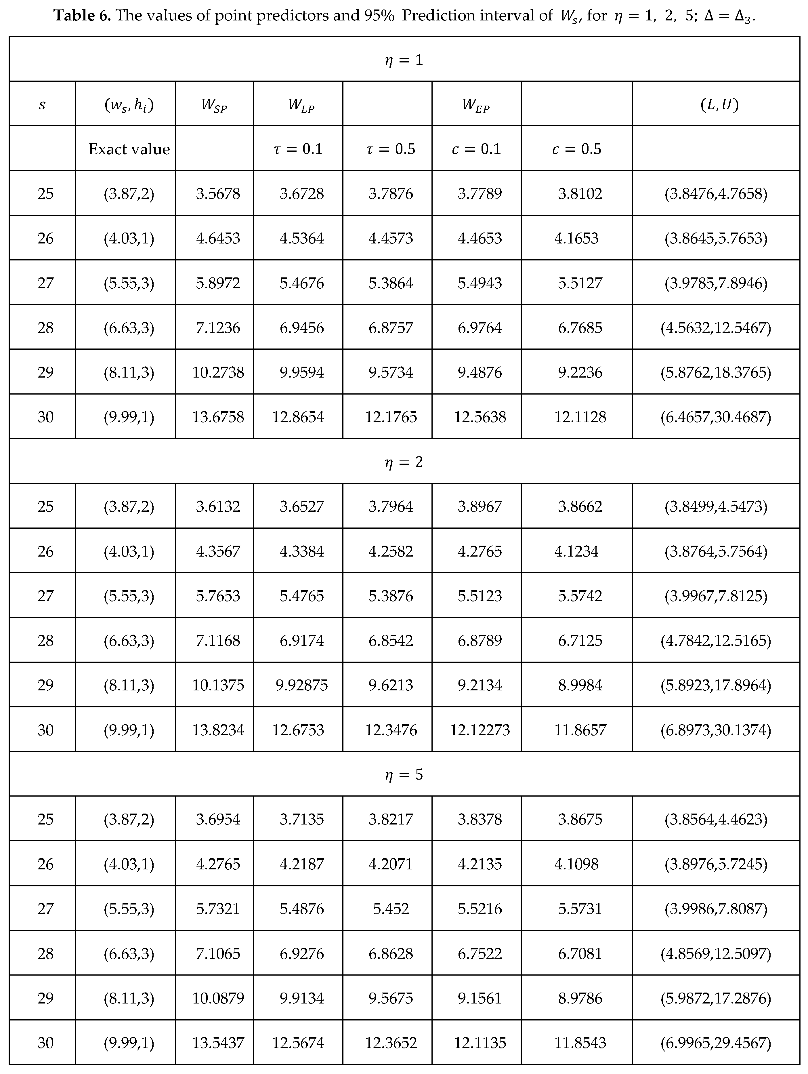
3.2. Illustrative example 

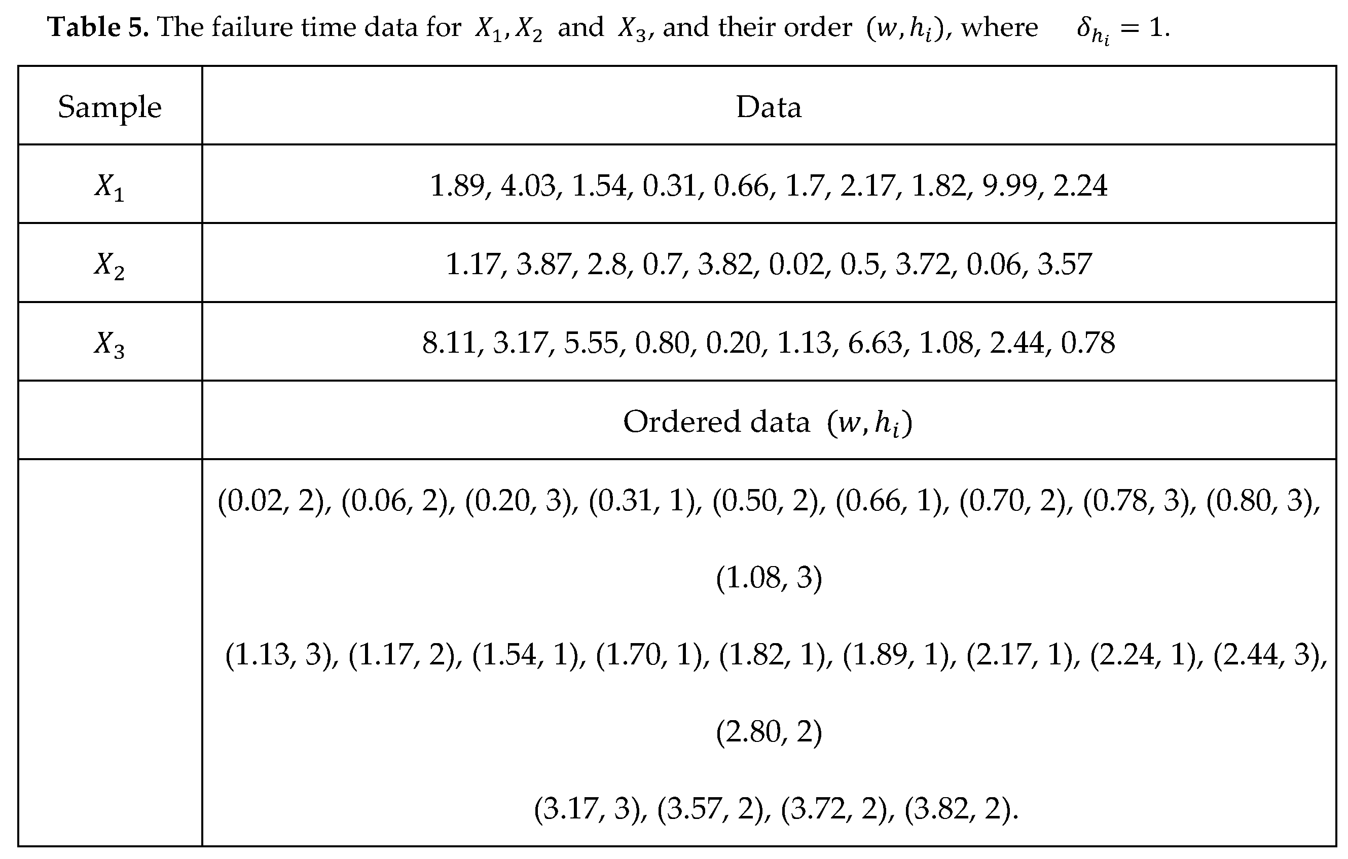
To illustrate the usefulness of the results developed in the previous sections, we consider three samples of size $n_1=n_2=n_3=10$ from Nelson's data (groups 1, 4, and 5) corresponding to the breakdown of an insulating fluid subjected to a high-stress load (see [20] p. 462), These breakdown times, referred to here as samples $X_i, i=\mathrm{1,2},3$, are jointly type-II censored data in the form of $(w,h_i)$ obtained from these three samples with $r=24$ and are shown in Table 5.

Using (16), (17), (18), (22), and (24), the MSPEs of the point predictors and prediction intervals of w_s, s = 25,..., 30 are calculated and presented in Table 6 using 𝜂 = 1, 2, 5 and Δ = Δ₃ = (1,2.6,1,2,1,3); 𝜏 = 0.1, 0.5 and c = 0.1, 0.5.

4. Conclusion

In this study, we considered a joint type- II censoring scheme in which the lifetimes of the three populations have exponential distributions. We determined the MSPEs of the point predictors and prediction intervals using different values for the learning rate parameter $\eta$ and different values for the parameters of the losses in both the simulation study and the illustrative example. From all tables in this prediction study, it can be seen that the results improve with increasing c, $\tau$ and $\eta$. In the simulation study, a comparison of the results in Tables 1 and 2 shows that the results in Table 1 are better, and the length of the prediction intervals in Table 4 is smaller than those in Table 3 because the observed values used in Table 3 are larger than those used in Table 4. The results of the illustrative example improve with larger values of c, $\tau$ and $\eta$. However, in both studies, the lengths of the prediction intervals increased as s increased. It may be interesting to examine this work using a different type of censoring.

References

- Bissiri, P. G., Holmes, C. C., and Walker, S. G. General framework for updating belief distributions. Journal of the Royal Statistical Society. Series B, Statistical Methodology, 2016, 78(5), 1103-1130. [CrossRef]
- Miller, J. W. and Dunson, D. B. Robust Bayesian inference via coarsening. Journal of the American Statistical Association, 2019, 114(527): 1113-1125. [CrossRef]
- Grünwald, P. (2012). The safe Bayesian: learning the learning rate via the mixability gap. In Algorithmic Learning Theory, 2012, volume 7568 of Lecture Notes in Computer Science, 169-183. Springer, Heidelberg. MR3042889.
- Grünwald, P. and van Ommen, T. Inconsistency of Bayesian inference for misspecified linear models, and a proposal for repairing it. Bayesian Analysis, 2017, 12(4): 1069-1103. [CrossRef]
- Grünwald, P. Safe probability. Journal of Statistical Planning and Inference, 2018, 47-63. MR3760837. [CrossRef]
- De Heide, R., Kirichenko, A., Grünwald, P., and Mehta, N. Safe-Bayesian generalized linear regression. In International Conference on Artificial Intelligence and Statistics, 2020, 2623-2633. PMLR. 106, 113.
- Holmes, C. C. and Walker, S. G. Assigning a value to a power likelihood in a general Bayesian model. Biometrika, 2017, 497-503. [CrossRef]
- Lyddon, S. P., Holmes, C. C., and Walker, S. G. General Bayesian updating and the loss-likelihood bootstrap. Biometrika, 2019, 465-478. [CrossRef]
- Martin, R. Invited comment on the article by van der Pas, Szabó, and van der Vaart. Bayesian Analysis, 2017, 1254-1258.
- Martin, R. and Ning, B. Empirical priors and coverage of posterior credible sets in a sparse normal mean model. Sankhy. Series A, 2020, 477-498. Special issue in memory of Jayanta K. Ghosh. [CrossRef]
- Abdel-Aty, Y., Kayid, M., and Alomani, G. Generalized Bayes estimation based on a joint type-II censored sample from k-exponential populations. Mathematics, 2023, 1-11. [CrossRef]
- Balakrishnana, N. and Rasouli, A. Exact likelihood inference for two exponential populations under joint Type-II censoring, Computational Statistics & Data Analysis, 2008. 2725-2738. [CrossRef]
- Parsi, S. Bairamov, I. Expected values of the number of failures for two populations under joint Type-II progressive censoring. Computational Statistics and Data Analysis, 2009, 3560-3570. [CrossRef]
- Rasouli, A., Balakrishnan, N. Exact likelihood inference for two exponential populations under joint progressive type-II censoring. Communications in Statistics - Theory and Methods, 2010, 2172-2191. [CrossRef]
- Su, F. Exact likelihood inference for multiple exponential populations under joint censoring. Open Access Dissertations and Theses, 2013, Ph.D Thesis, McMaster University.
- Abdel-Aty, Y. Exact likelihood inference for two populations from two-parameter exponential distributions under joint Type-II censoring, Communications in Statistics - Theory and Methods, 2017, 9026-9041. [CrossRef]
- Shafay, A.R., Balakrishnan, N. Y. Abdel-Aty, Y. Bayesian inference based on a jointly type-II censored sample from two exponential populations, Journal of Statistical Computation and Simulation, 2014, 2427-2440. [CrossRef]
- Asgharzadeh, A., Valiollahi, R. and Kundu, D. Prediction for future failures in Weibull distribution under hybrid censoring. Journal of Statistical Computation and Simulation, 2013, 824-838. [CrossRef]
- Abdel-Aty, Y., Franz, J., Mahmoud, M.A.W. Bayesian prediction based on generalized order statistics using multiply type-II censoring. Statistics, 2007, 495-504. [CrossRef]
- Nelson, W. Applied Life Data Analysis; Wiley: New York, NY, USA, 1982.
Disclaimer/Publisher’s Note: The statements, opinions and data contained in all publications are solely those of the individual author(s) and contributor(s) and not of MDPI and/or the editor(s). MDPI and/or the editor(s) disclaim responsibility for any injury to people or property resulting from any ideas, methods, instructions or products referred to in the content. |
© 2023 by the authors. Licensee MDPI, Basel, Switzerland. This article is an open access article distributed under the terms and conditions of the Creative Commons Attribution (CC BY) license (http://creativecommons.org/licenses/by/4.0/).
Copyright: This open access article is published under a Creative Commons CC BY 4.0 license, which permit the free download, distribution, and reuse, provided that the author and preprint are cited in any reuse.