
Submitted:
21 December 2023
Posted:
25 December 2023
You are already at the latest version
Abstract
Well deliverability optimization is essential for oil and gas production and nodal analysis is a common tool used for selecting suitable production parameters. To accurately calculate upstream and downstream pressures at various production rates at a certain selected node, proper modeling of multiphase flow in wellbores is necessary. However, this process is complex due to the inconsistent velocities of the fluids (i.e., oil, gas, and water) and the interaction between the liquids under high temperature and pressure. Empirical models, such as Hagedorn and Brown (1965), Beggs and Brill (1973), and Mukherjee and Brill (1983 and 1985), and the drift-flux model (Zuber 1965) are commonly used for multiphase flow calculations in wellbores. In this paper, we programmed and evaluated three multiphase flow models (Hagedorn-Brown, Mukherjee-Brill, and drift-flux) using Matlab. The programming includes holdup calculation, pressure gradient calculation, pressure traverse calculation, inflow curve determination, inflow performance relationship (IPR) curve determination, and well deliverability determination. Additionally, we conducted a case study to examine the sensitivity of parameters and compare and analyze the results of pressure traverse, tubing intake curve, and deliverability determination between the drift-flux and Mukherjee-Brill models. Sensitivity analysis was conducted on two of the seven parameters in the drift-flux model, and the effects of production and reservoir parameters on well deliverability were analyzed. The case study results indicated that the Mukherjee-Brill model predicted slightly higher bottomhole pressure compared to the drift-flux model at a fixed oil flow rate, but its well deliverability determination was lower. Furthermore, the drift-flux model showed that the pressure increased with an increase in the distribution coefficient for bubble flow (C0_bubble), while the beta parameter had little impact on the calculated pressure in the studied range. The well deliverability increased when the tubing size and reservoir pressure increased, or the tubing head pressure decreased.
Keywords:
Multiphase flow
; Drift-flux model
; Matlab programming
; Nodal analysis
; Production engineering.
1. Introduction
Liquid holdup phenomena occur in two-phase flow due to the inconsistence in velocities of the liquid and gas. Because gas has a lower viscosity than liquid, the cross sectional area occupied by gas will be less than that occupied by liquid. Consequently, liquid will be held up in a vertical production well. The fluid properties of the mixture, such as the density and viscosity can be significantly changed with/without liquid holdup. Therefore, the accurate prediction of liquid holdup is of great importance in determining the pressure drop in a two-phase flow in the tubing.
Hagedorn and Brown (1965) did experiments in a 1500 ft vertical well to study the pressure drop due to two-phase flow in a small diameter tubing. Based on the experimental data, they developed correlations to accurately predict the pressure gradient in different tubings, through different flow regimes. In practice, we can calculate the liquid and gas holdups using three charts with a few dimensionless numbers or using fitted equations based on these charts. The drawback of Hagedorn and Brown is that it was developed and only valid for vertical well.
Beggs and Brill (1973) correlation is another useful tool to calculate the liquid holdup and pressure drop for two-phase flow in pipes. They were developed using experimental data in transparent acrylic pipes (2.5 and 3.8 cm in diameter) with different inclination angles. Three flow patterns, i.e., segregated flow, distributed flow, and intermittent flow were categorized. The liquid holdup was correlated for horizontal holdup and holdup at a specific angle.
Mukherjee and Brill (1983 and 1985) developed another holdup and pressure drop calculation for multiphase flow based on curve fitting the measured data. Besides the dimensionless numbers adopted by Duns & Ros (1963), three more dimensionless numbers were defined to characterize the boundary transitions. The flow patterns and their boundaries were determined using the dimensionless numbers obtained. The flow regime included bubble flow, slug flow, annular mist flow and stratified flow. A mechanistic model was developed for the stratified flow only.
The Tulsa University Fluid Flow Projects (TUFFP) published a large amount of experimental data for multiphase flow and a number of models were developed based on those data (Felizola and Shoham, 1995; Gomez et al. 1999). These models showed good performance in pressure drop calculation. These unified models are out of the scope of this project and will not be included.
2. Theoretical Introduction of Drift-Flux Model
The drift flux method was first introduced by Zuber and Findlay (1965) and adopted in the work of Shi et al. (2005a and 2005b). There are two mechanisms for the slip in the drift-flux model for two-phase flow. The first one is based on the fact that gas concentration is the highest at the centre. The other mechanism is associated with the faster velocity of gas through liquid due to the density difference. The gas velocity was correlated with the drift velocity and mixture velocity in equation 1:
 Where, is the gas velocity, is the drift velocity, is the distribution coefficient, is the average mixture velocity.
The distribution coefficient is about 1.2 for bubble flow while its correlation proposed was by Shi et al. (2005b) as follows,
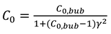 Where, and . is the flooding velocity which is sufficient to hold a liquid film around the annulus.
The gas flooding velocity was defined by Wallis and Makkenchery (1974) and can be expressed as
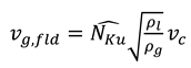 Where, is the critical velocity and is the critical Kutateladze number which can be correlated to the modified pipe diameter number by using equation
 Where, .
The drift velocity is determined by equation 5.
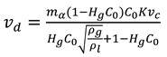 Where, = and
The gas hold up can be calculated using equation 6.
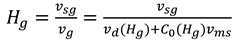
There are seven parameters in the drift flux model and they were optimized depending on the pipe diameter based on the experimental data in Table 1.
Compared to the Mukherjee and Brill model, drift-flux model is easy to follow and can be easily coupled with commercial reservoir simulators (CMG or Eclipse). Mukherjee and Brill model can give detailed flow regime predictions which makes this model easy to validate.
3. Methodology
3.1. Liquid and gas holdups calculation
The first step to program the drift-flux model is the liquid and gas holdups calculation. Depending on the size of the pipe diameter d, one of the two sets of parameters will be chosen. The calculation requires a first guess on gas holdup before other parameters, such as critical velocity the critical Kutateladze number can be calculated. The input value λg can be used for the initialization of gas holdup. vc, Nd, Nku will be calculated based on the guess of the gas holdup. The drift velocity vd can be calculated using the values of β, γ, C0.
Then the gas holdup can be determined in an iterative manner because drift velocity and other parameters depend on the new value of the gas holdup. The gas holdup can be updated in equation 7 using Picard iteration with a damping factor.

The detailed calculation can be summarized in the flow chart in Figure 1.
3.2. Pressure Gradient Calculation
After the liquid and gas holdups are determined, pressure drop and traverse calculations can be done using the method in the Hagedorn and Brown model. Specifically, Reynolds number and mixture density, viscosity, dimensionless kinetic energy are determined using equations 8-11.
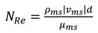


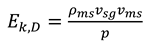
The friction factor will be determined using the correlation which is developed by curve fitting the Moody chart. The pressure gradient is determined by using equation 12.

3.3. Pressure Traverse Calculation
The pressure traverse, which is the pressure as a function of the distance along the wellbore, can be calculated by applying the ode45 function in Matlab which integrates the pressure drop at different locations. In this project, Dr. Jansen’s code example_traverse.m was modified for pressure traverse calculation.
3.4. Intake Curve
The intake curve depicts the pressure vs flow rate curve at the selected node. The pressure traverse can be calculated at different production rates, then the intake curve can be determined. In this project, Dr. Jansen’s code example_intake_curve.m was modified for intake curve determination.
3.4. Inflow Performance Relationship (IPR) Curve
IPR relates the bottomhole pressure to the flow rate using the upstream calculation. Vogel method (1968) is commonly used for IPR calculation which can be represented in equation 10.

In this project, Dr. Jansen’s code res_Vogel.m was used for IPR curve determination.
3.5. Well Deliverability Determination
When IPR curve and intake curve are plotted on the same figure, the well deliverability can be determined at the intersection.
3.6. Same Caveats in Coding in Matlab
3.6.1. The ode45 Function
The ode45 only accepts four arguments (odefun,tspan,y0,options) according to the Matlab’s manual while ode45 function takes 14 arguments in Dr. Jansen’s pipe.m file. This is because historically Matlab didn’t have function handles. Detailed explanation can be found on Matlab answer central (2019). If Matlab decides to make change to ode45 function at some point, the codes from Dr. Jansen may stop working.
3.6.2. The deal Function
If multiple variables need assignment, deal function in Matlab can be used. This function makes our code neat because we need to assign many values to the variables quite often. For example, there are seven parameters in drift flux model and we can assign all the values at once by using [C0_bub, beta_,a1,a2,m0,n1,n2]=deal(1,1,0.06,0.21,1.85,0.21,0.95).
3.6.3. Equation 7
In equation 7, and mean that they are function of the gas holdup, so it’s important that we don’t multiply to them in coding.
3.6.4. Vectors and Scalars
It is important to differentiate vectors and scalars used in the functions. For example, a function named local_gas_oil_water_props needs to be programed to have viscosity and flow rate as vectors.
4. Results and Discussion
The basic parameters used for the multiphase flow and IPR calculations are listed in Table 2 and Table 3. These parameters were taken from Dr. Jansen’s book.
4.1. Results from Drift Flux Model
4.1.1. Pressure Traverse
The pressure traverse along the wellbore calculated using the drift-flux model is shown in Figure 2. The acceleration term is very small while the gravity loss contributes the most pressure drop. The pressure drop due to friction is significant when the flow is near the wellhead. This is because a high gas flow rate will cause a high friction at a low pressure near the wellhead.
4.1.2. Intake Curve
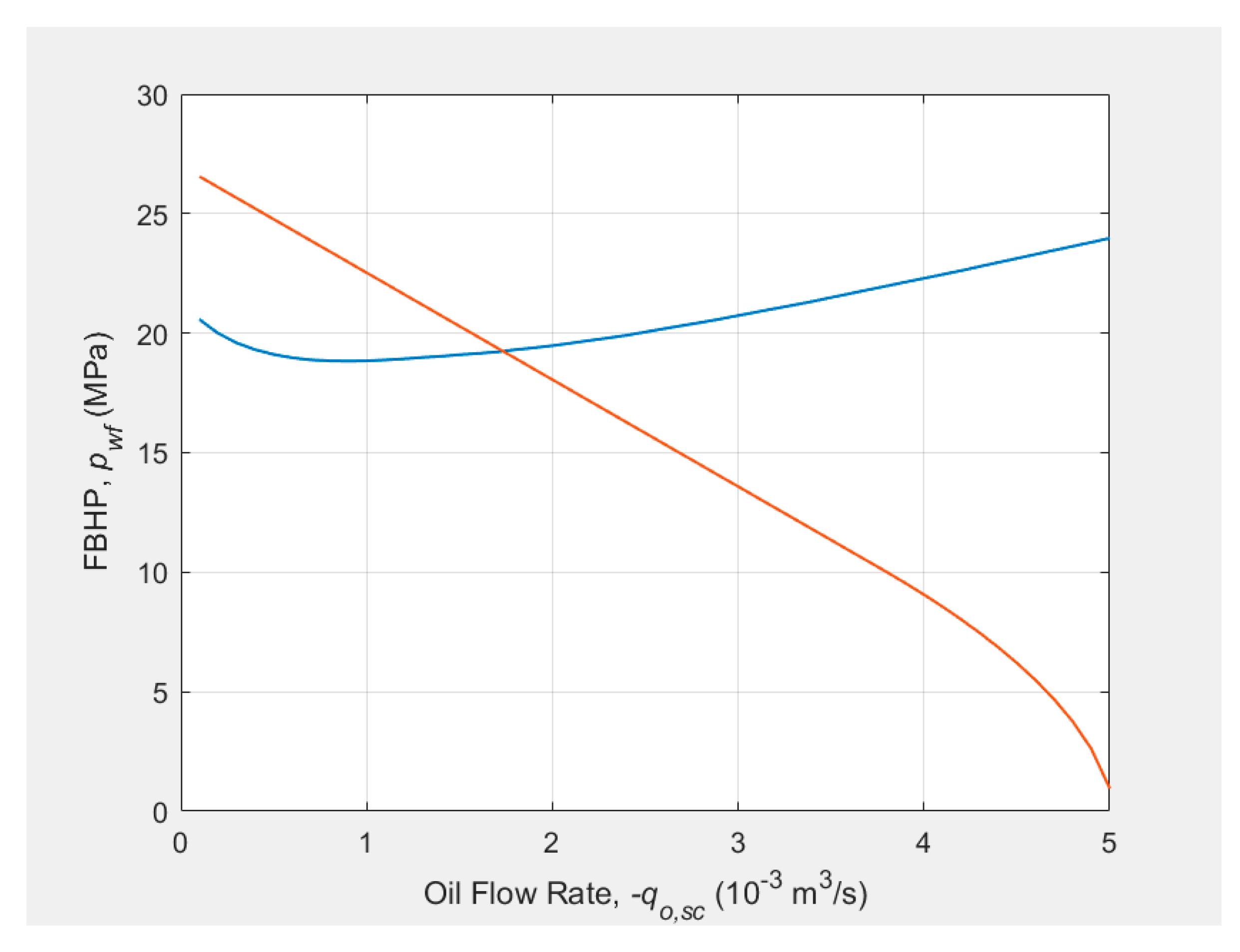
The tubing intake curve or the vertical lifting performance (VLP) curve calculated using the drift-flux model is plotted in Figure 3. The bottomhole pressure decreases with the oil production rate when the rate is low while it increases with the oil production rate when the rate is high. The mixture density increases with the decrease of flow rate at the low flow region which causes the gravity loss to be large. Thus the bottomhole pressure increases when the flow rate decreases at the low flow region. Friction loss will dominate the pressure drop when the flow rate is high which leads to the increase of bottomhole pressure.
4.1.3. Well Deliverability
The well deliverability is determined by plotting the IPR curve and the tubing intake curve calculated by using the drift-flux model. It is determined to be 1.7×10⁻³ m3/s.
Figure 3.
The well deliverability determined by using drift-flux model.
4.2. Compare with Mukherjee-Brill Method
4.2.1. Pressure Traverse
Pressure traverses calculated using M-B (dashed line) and drift-flux (solid line) models are plotted in Figure 4. The M-B model gives a slightly higher pressure at each location.
4.2.2. Intake Curve
The tubing intake curves calculated using M-B and drift-flux models are plotted in Figure 5. The bottomhole pressure calculated using M-B model is higher than that from drift-flux model.
4.2.3. Well Deliverability
The well deliverabilities determined by using M-B and drift-flux models are plotted in Figure 6. The M-B model gives a higher well deliverability (1.7×10⁻³ m3/s) than that determined by using drift-flux model (1.4×10⁻³ m3/s).
4.3. Effect of Main Parameters in the Drift Flux Model
4.3.1. Distribution Coefficient C0_bubble
The pressure traverses at three different distribution coefficient C0_bubble (0.5, 1, 2) are plotted in Figure 7. With the increase of the distribution coefficient, there is a slight increase in wellbore pressure.
4.3.2. Parameter
The pressure traverses at three different Parameter (0.6, 1, 2) are plotted in Figure 8. There is almost no impact of this parameter on the pressure traverse.
4.4. Parameters Affecting the Well Deliverability
4.4.1. Tubing Head Pressure
Three tubing intake curves with three tubing head pressure (0.5, 1, and 2 MPa) as well as the IPR curve are plotted in Figure 9. It can be seen that the well deliverability increases with the decrease of the tubing head pressure.
4.4.2. Tubing Size
Three tubing intake curves with three tubing size (0.05, 0.062, and 0.1 m) as well as the IPR curve are plotted in Figure 10. It can be seen that the well deliverability increases with the increase of the tubing size.
4.4.3. Reservoir Pressure
Three IPR curves with three reservoir pressures (27, 30 and 35 MPa) as well as the tubing intake curve are plotted in Figure 11. It can be seen that the well deliverability increases with the increase of the reservoir pressure. The higher operational oil flow rate is caused by higher driving force provided by the higher reservoir pressure.
5. Conclusions
In this study, the theoretical background of drift-flux model and the methodology of coding the model for holdup, pressure traverse, intake curve and well deliverability calculations in Matlab were presented. The results predicted from Mukherjee-Brill model and the drift-flux model were compared. The effects of the main parameters of the model were discussed. The effects of production and reservoir parameters on the well deliverability were analyzed. The major conclusions and remarks from this study are:
1. The predicted bottomhole pressure from the Mukherjee-Brill model was higher than that from the drift-flux model at a fixed oil flow rate;
2. The well deliverability determined using drift-flux model was higher than that from the Mukherjee-Brill model.
3. With the increase of the distribution coefficient, there is a slight increase in wellbore pressure; while the Parameter has little impact on the pressure calculation;
4. The well deliverability increased when the tubing size and reservoir pressure increased or the tubing head pressure decreased;
5. It should be noted that the conclusions were based on the case study with fixed parameters; therefore, cautions should be taken to generalize the results to other cases;
6. Matlab coding has been put into practice for multiphase flow calculations through this course project;
7. Well production optimization using nodal analysis has been achieved using Matlab code.
References
- Beggs, H.D. and Brill, J.P. 1973. A Study of Two-Phase Flow in Inclined Pipes. J. Pet. Technol 25(05): 607–617. [CrossRef]
- Duns, Jr. and Ros, N.C.J. 1963. Vertical Flow of Gas and Liquid Mixtures in Wells. Paper presented at 6th World Petroleum Congress. Frankfurt, 19-26 June 1963.
- Felizola, H. , and Shoham, O. 1995. A Unified Model for Slug Flow in Upward Inclined Pipes. ASME. J. Energy Resour. Technol. [CrossRef]
- Gomez, L. E., Shoham, O., Schmidt, Z., Chokshi, R. N., Brown, A., and T. Northug. 1999. A Unified Mechanistic Model for Steady-State Two-Phase Flow in Wellbores and Pipelines. Paper presented at the SPE Annual Technical Conference and Exhibition, Houston, Texas. [CrossRef]
- Hagedorn, A.R. and Brown, K.E. 1965. Experimental Study of Pressure Gradients Occurring during Continuous Two-Phase Flow in Small-Diameter Vertical Conduits. J. Pet. Technol., 17(04): 475-484. [CrossRef]
- Jansen, J.D. 2017. Nodal Analysis of Oil and Gas Production Systems. Society of Petroleum Engineers. [CrossRef]
- Matlab answer central 2019. https://www.mathworks.com/matlabcentral/answers/469314-ode45-varargin-additional-arguments-after-options.
- Mukherjee, H., and Brill J.P. 1983. Liquid Holdup Correlations for Inclined Two-Phase Flow. J Pet Technol 35(1983): 1003–1008. [CrossRef]
- Mukherjee, H.; Brill, J.P. Empirical equations to predict flow patterns in two-phase inclined flow. International Journal of Multiphase Flow 1985, 11, 299–315. [Google Scholar] [CrossRef]
- Wallis, G.B. and Makkenchery, S. 1974. The hanging film phenomenon in vertical annular two-phase flow. J. Fluids Eng 96(3): 297-298. [CrossRef]
- Shi, H., Holmes, J.A., Diaz, L.R. Durlofsky, L.J., Aziz, K. 2005a. Drift-Flux Parameters for Three-Phase Steady-State Flow in Wellbores. SPE J., 10 (2): 130-137. [CrossRef]
- Shi, H., Holmes, J.A. Durlofsky, L.J., Aziz, K., Diaz, L.R., Alkaya, B., Oddie, G. 2005b. Drift-Flux Modeling of Two-Phase Flow in Wellbores. SPE J. 10 (1): 24-33. [CrossRef]
- Zhang, H., Wang, Q., Sarica, C., and Brill, J. P. 2003. Unified Model for Gas-Liquid Pipe Flow via Slug Dynamics—Part 1: Model Development. ASME. J. Energy Resour. Technol. 125(4): 266–273. [CrossRef]
- Zuber, N. and Findlay, J.A. (1965) Average Volumetric Concentration in Two-Phase Flow Systems. Journal of Heat Transfer, 87, 453-468. [CrossRef]
Figure 1.
Flowchart to calculate holdups using drift flux model.
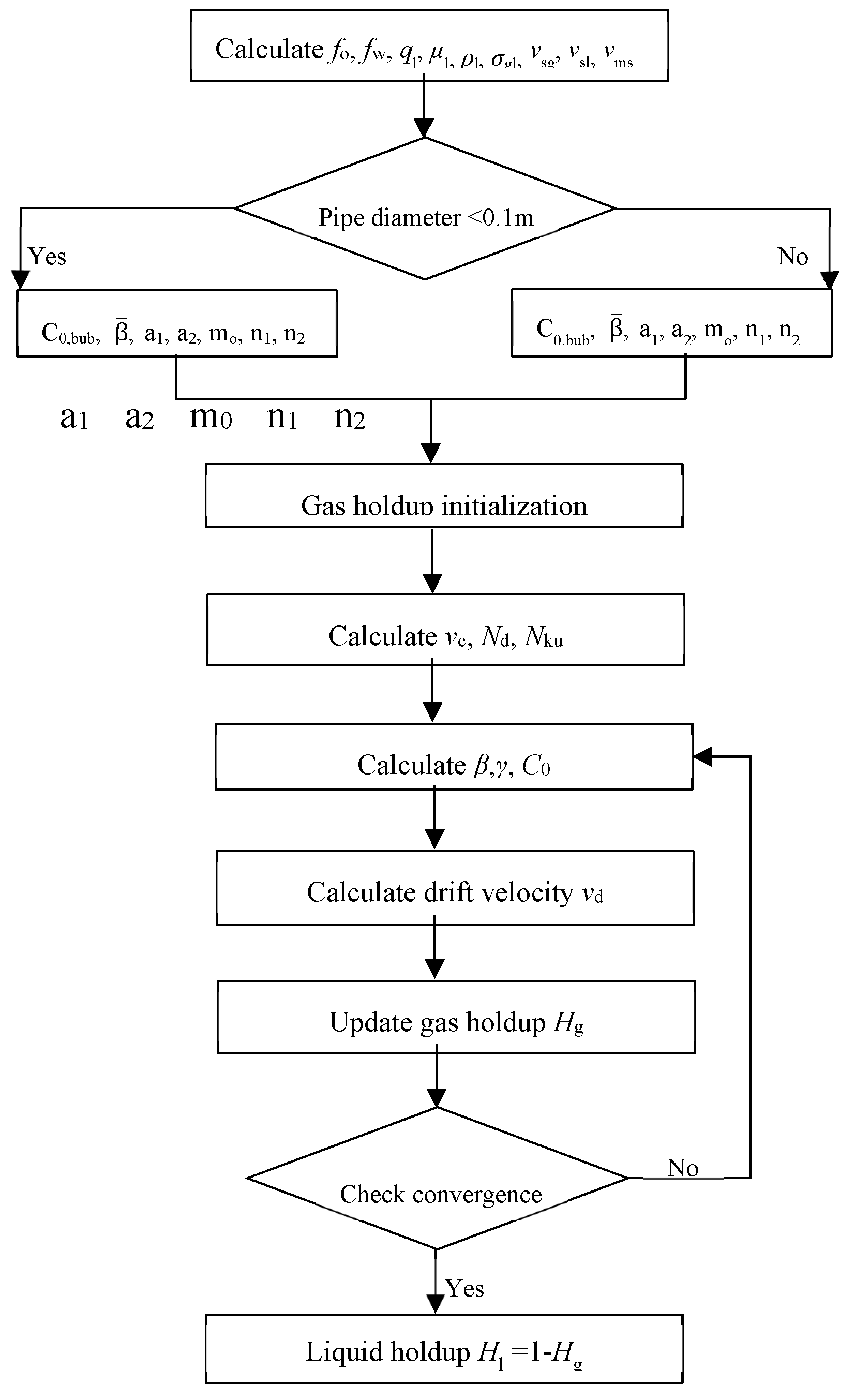
Figure 2.
Pressure traverse calculated using drift-flux model.
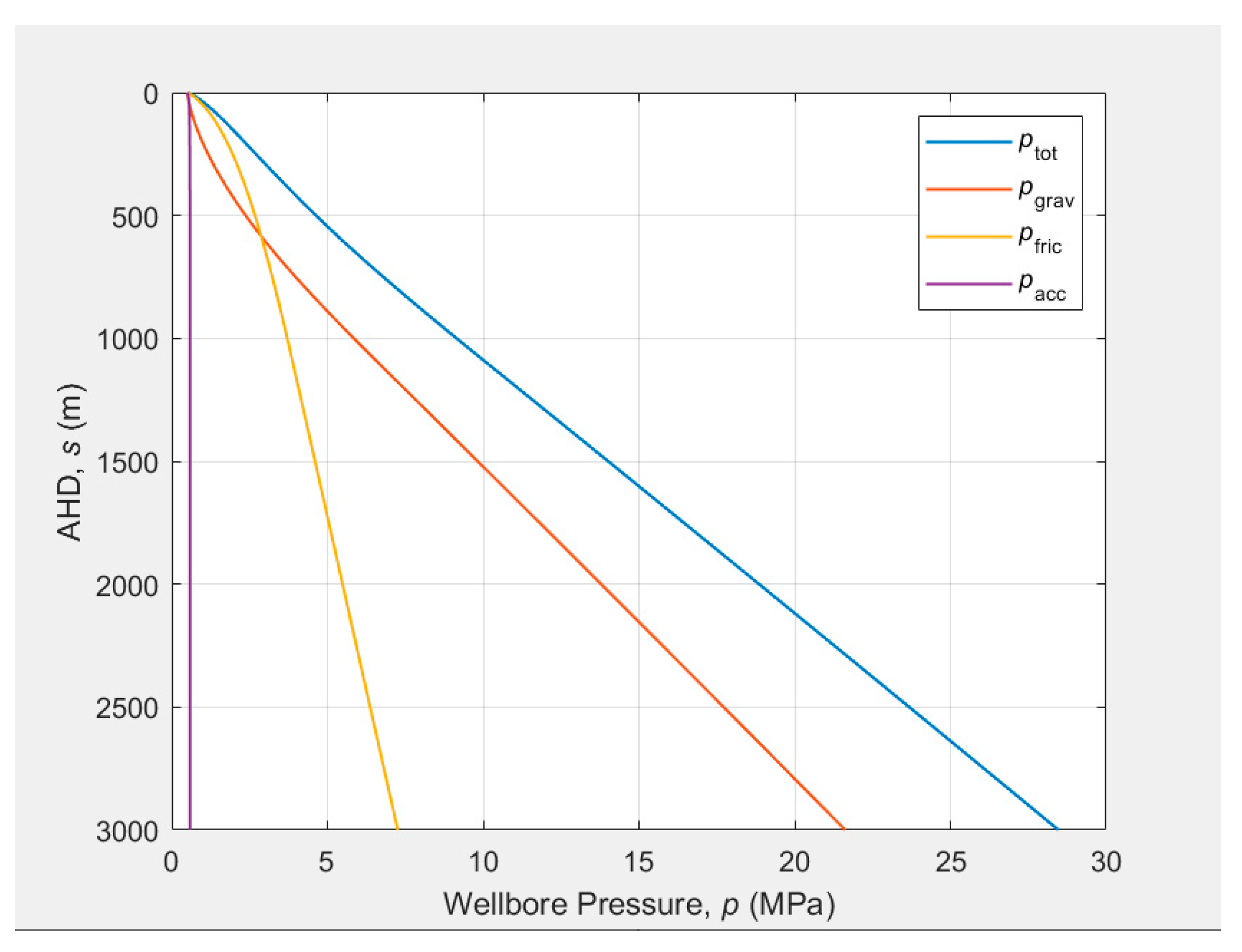
Figure 3.
The tubing intake curve calculated using drift-flux model.
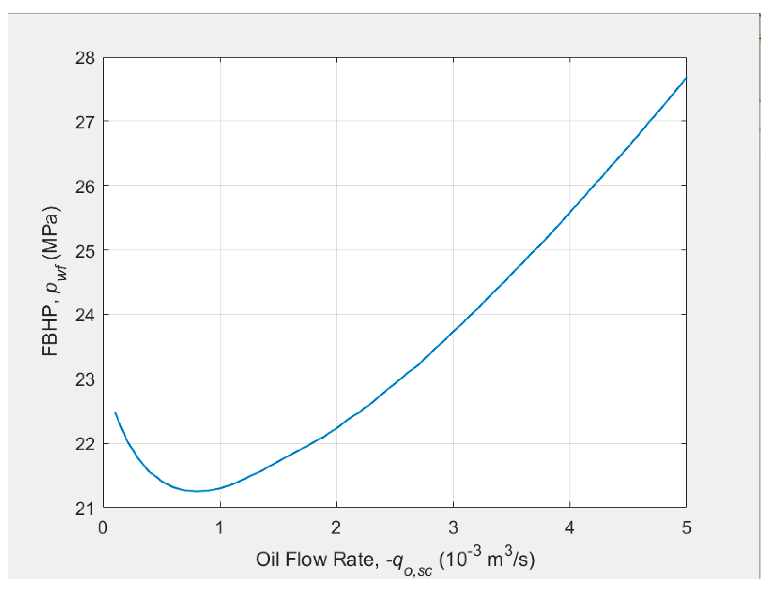
Figure 4.
Pressure traverses calculated using M-B and drift-flux models.
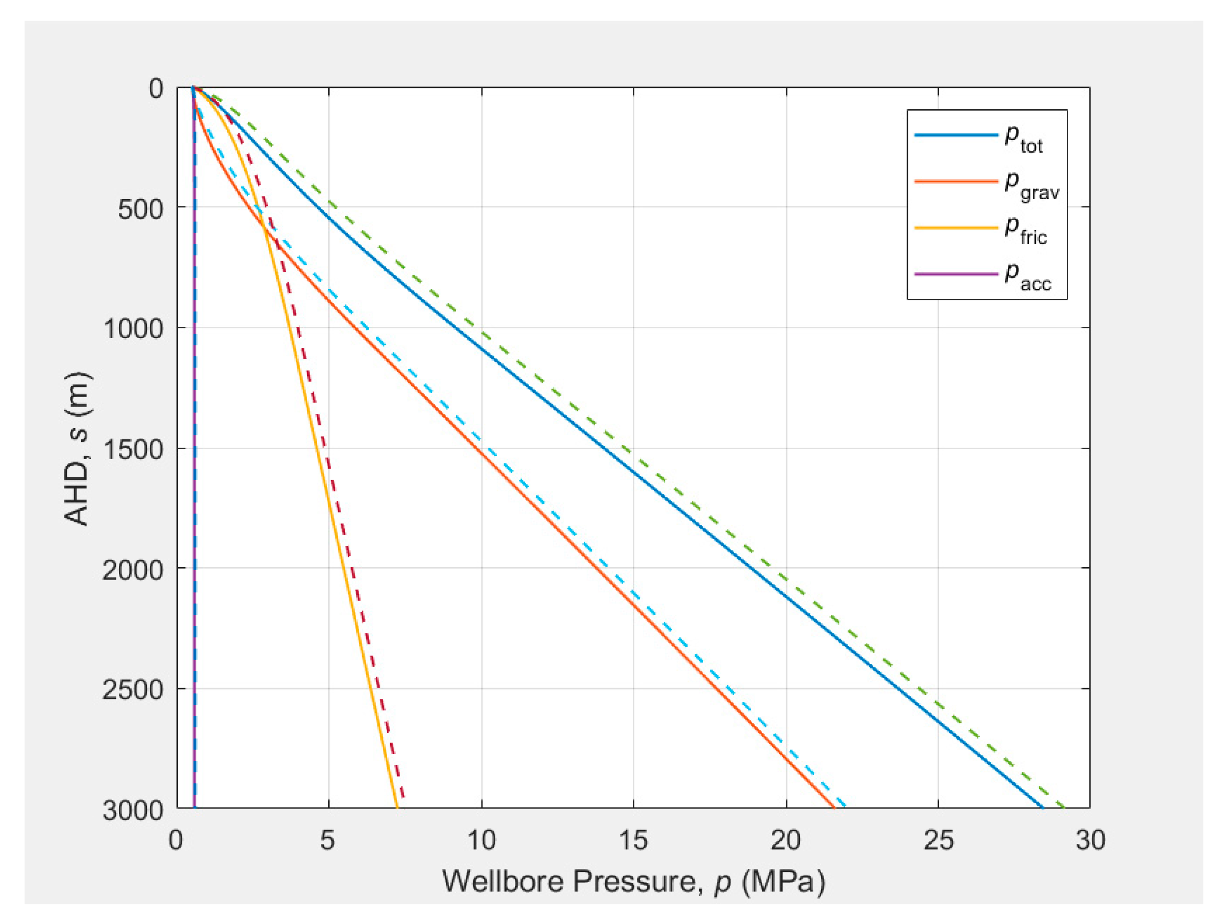
Figure 5.
The tubing intake curves calculated using M-B and drift-flux models.
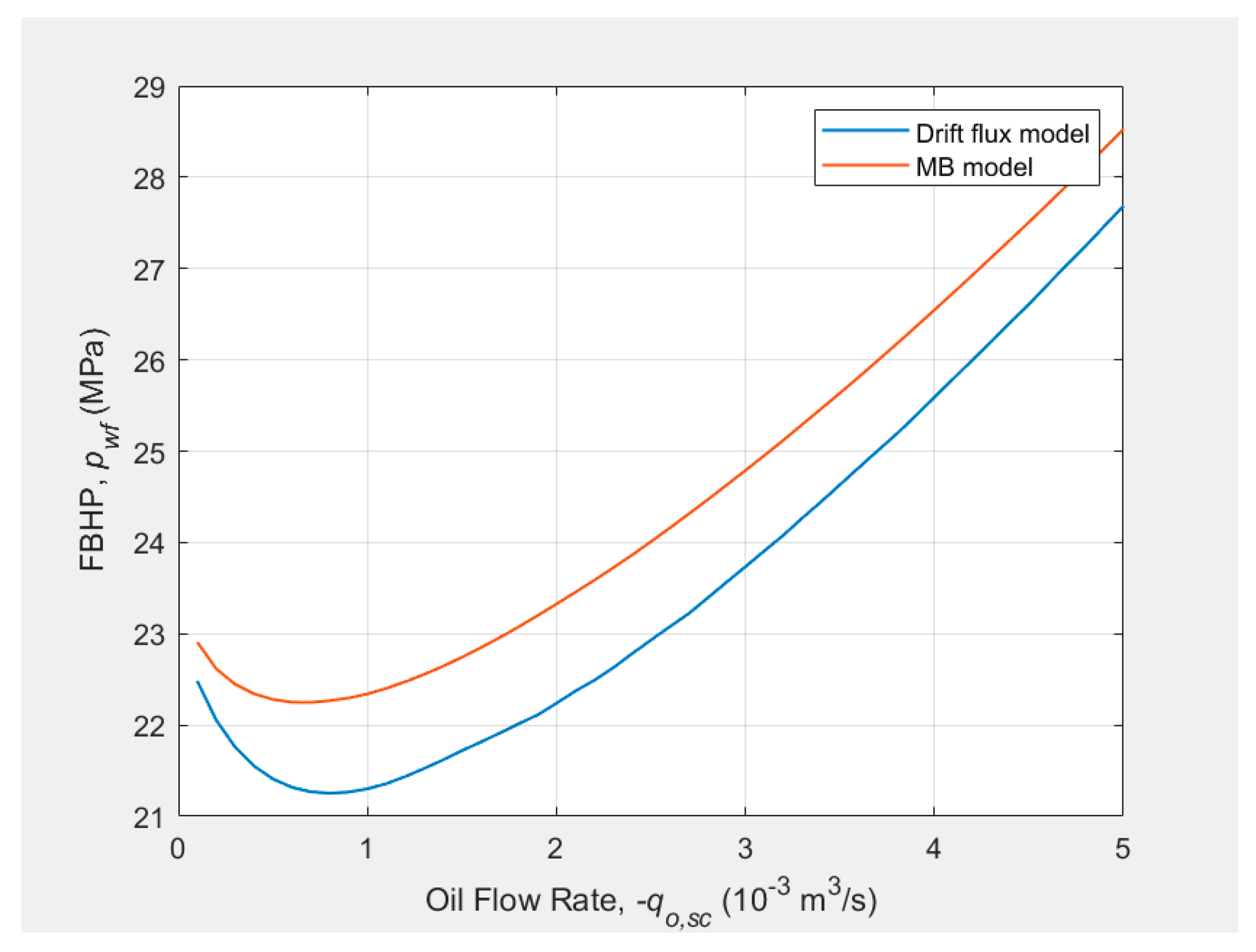
Figure 6.
The well deliverabilities determined by using M-B and drift-flux models.
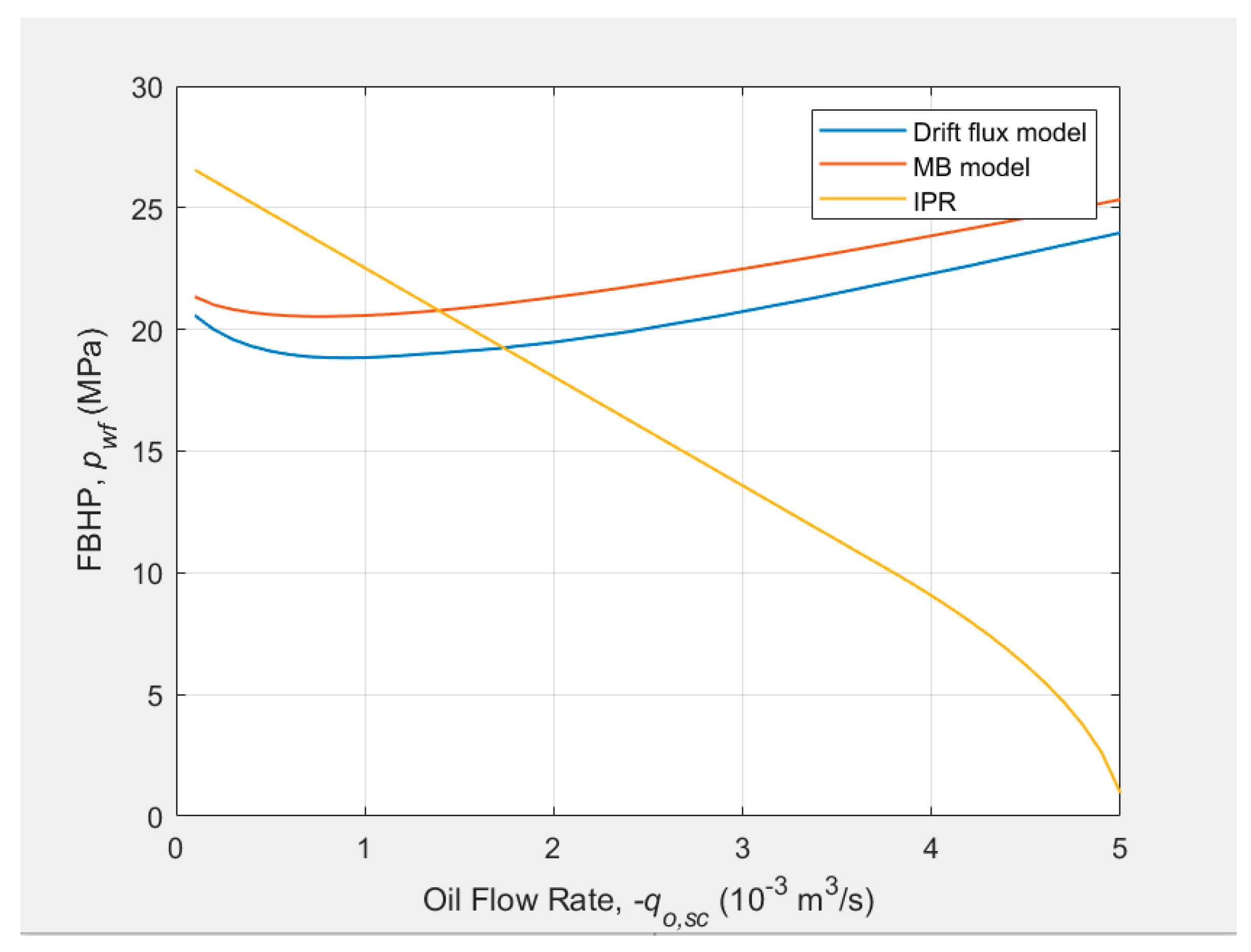
Figure 7.
The pressure traverses at three different distribution coefficient C0_bubble.
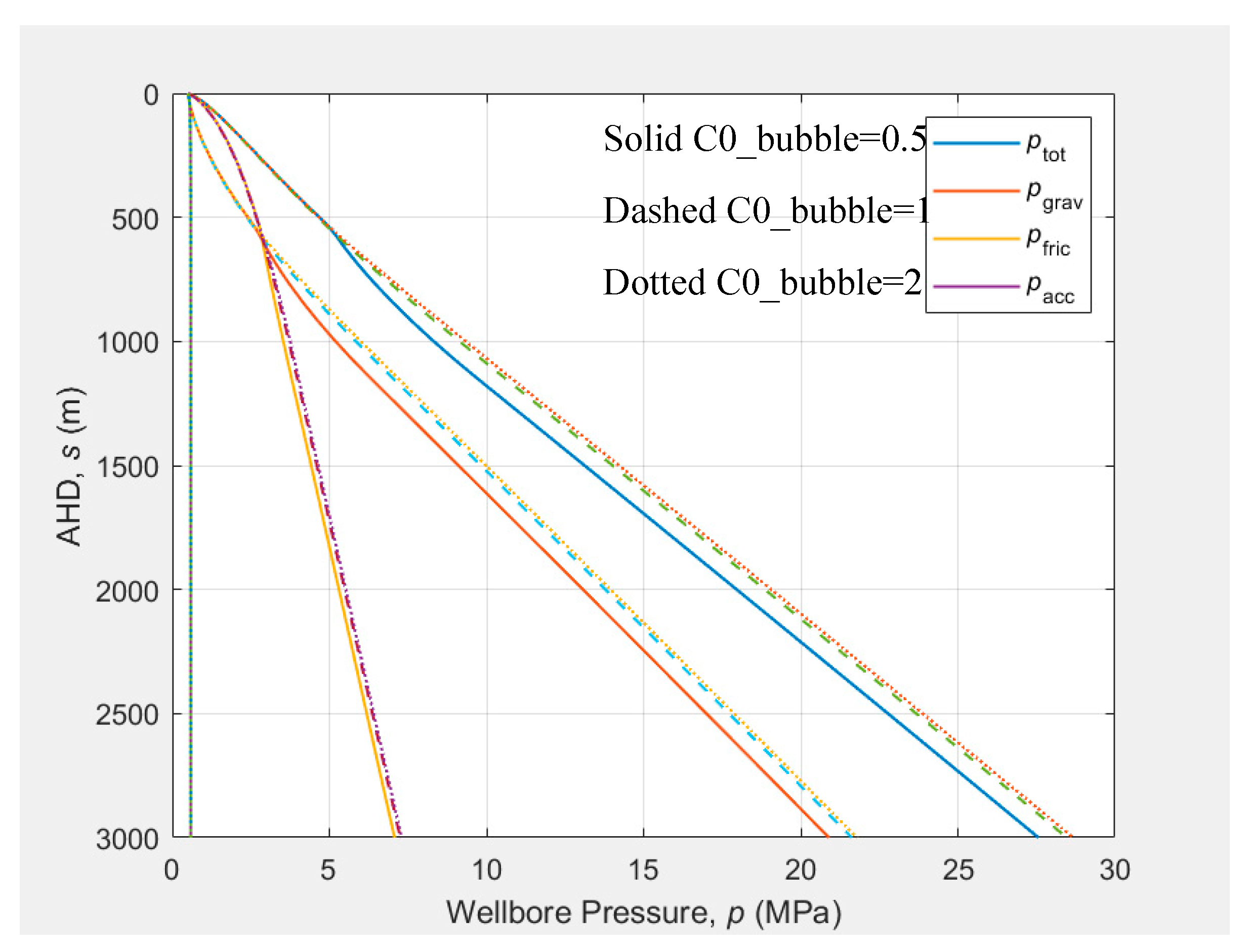
Figure 8.
The pressure traverses at three different Parameter .
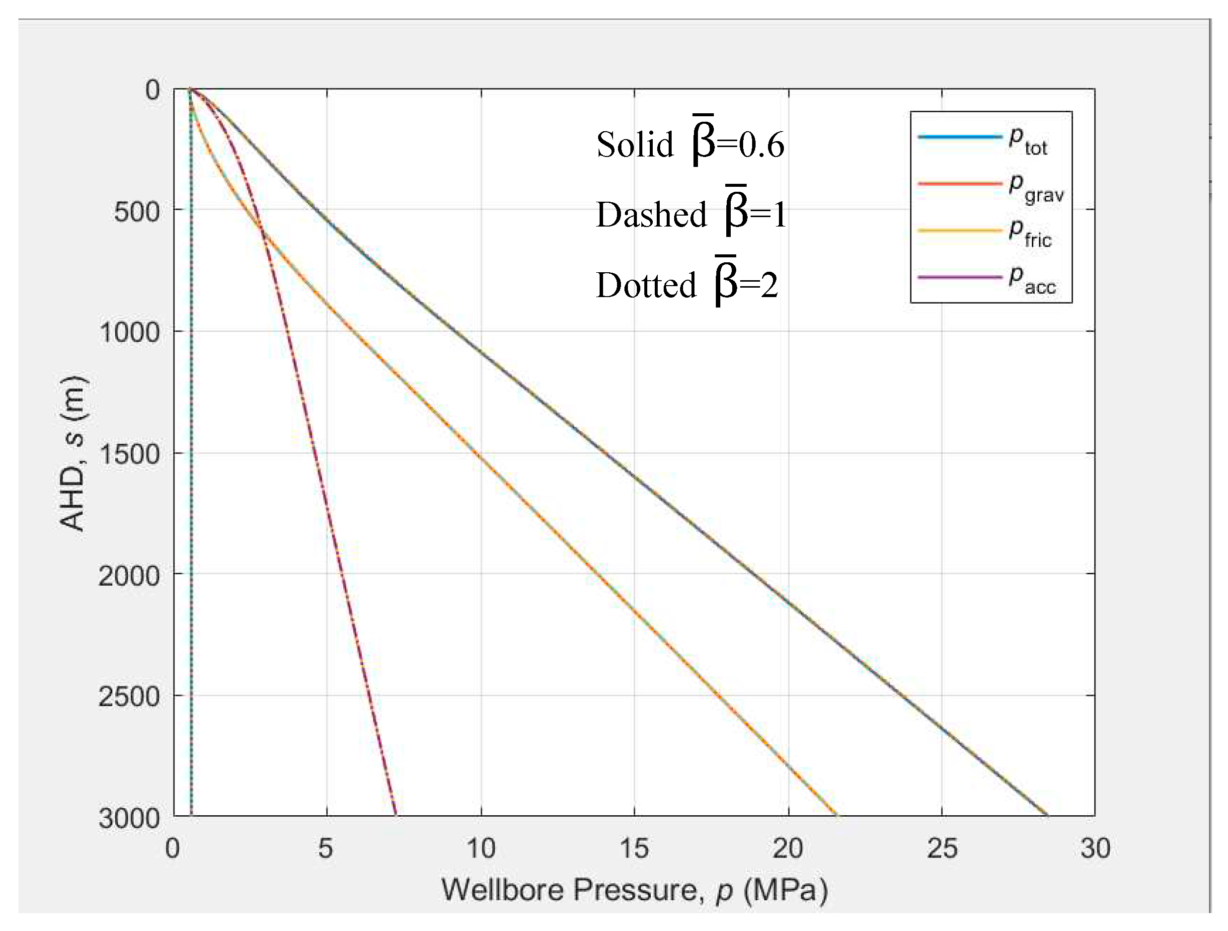
Figure 9.
Effect of tubing head pressure on the well deliverability.
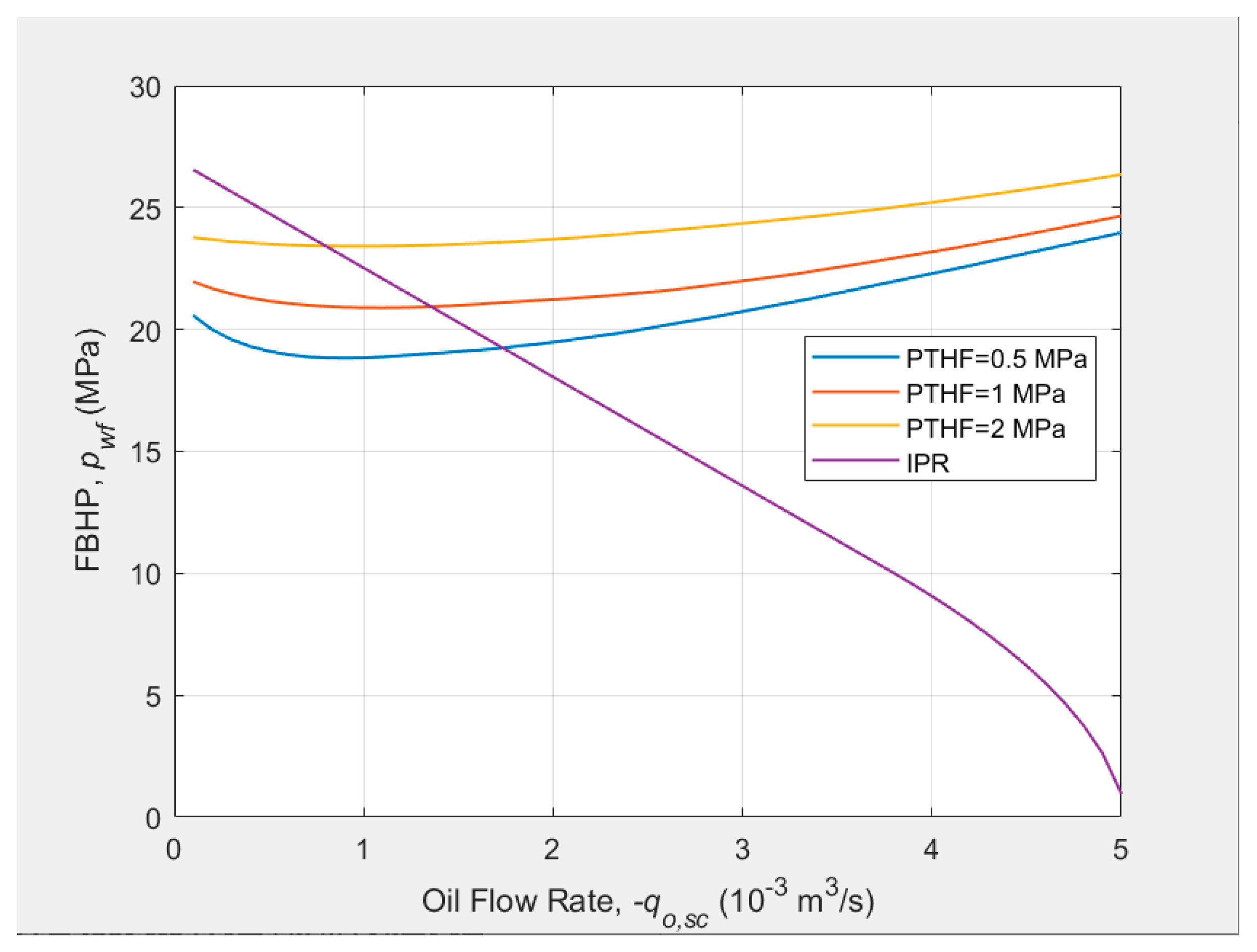
Figure 10.
Effect of the tubing size on the well deliverability.
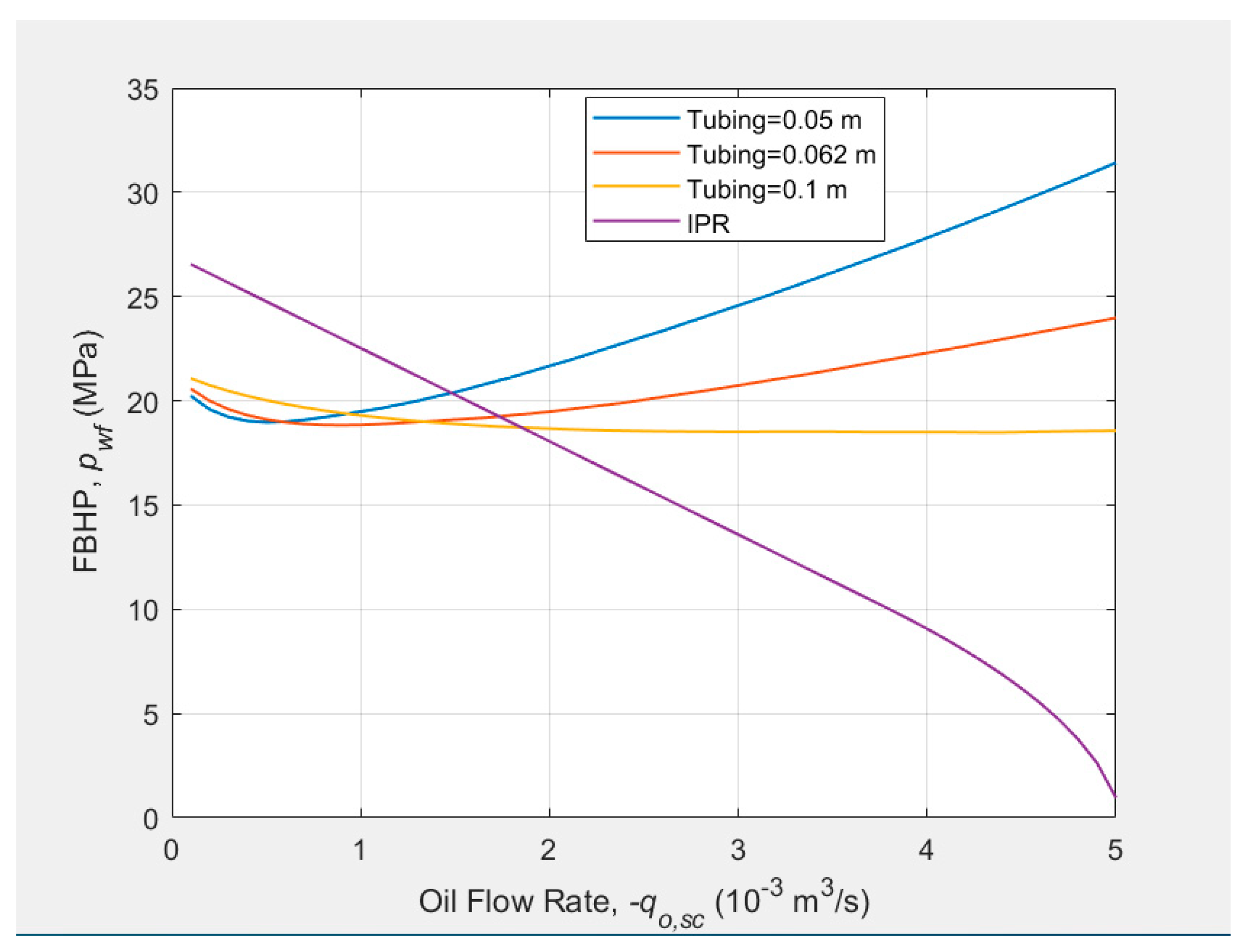
Figure 11.
Effect of the reservoir pressure on the well deliverability.
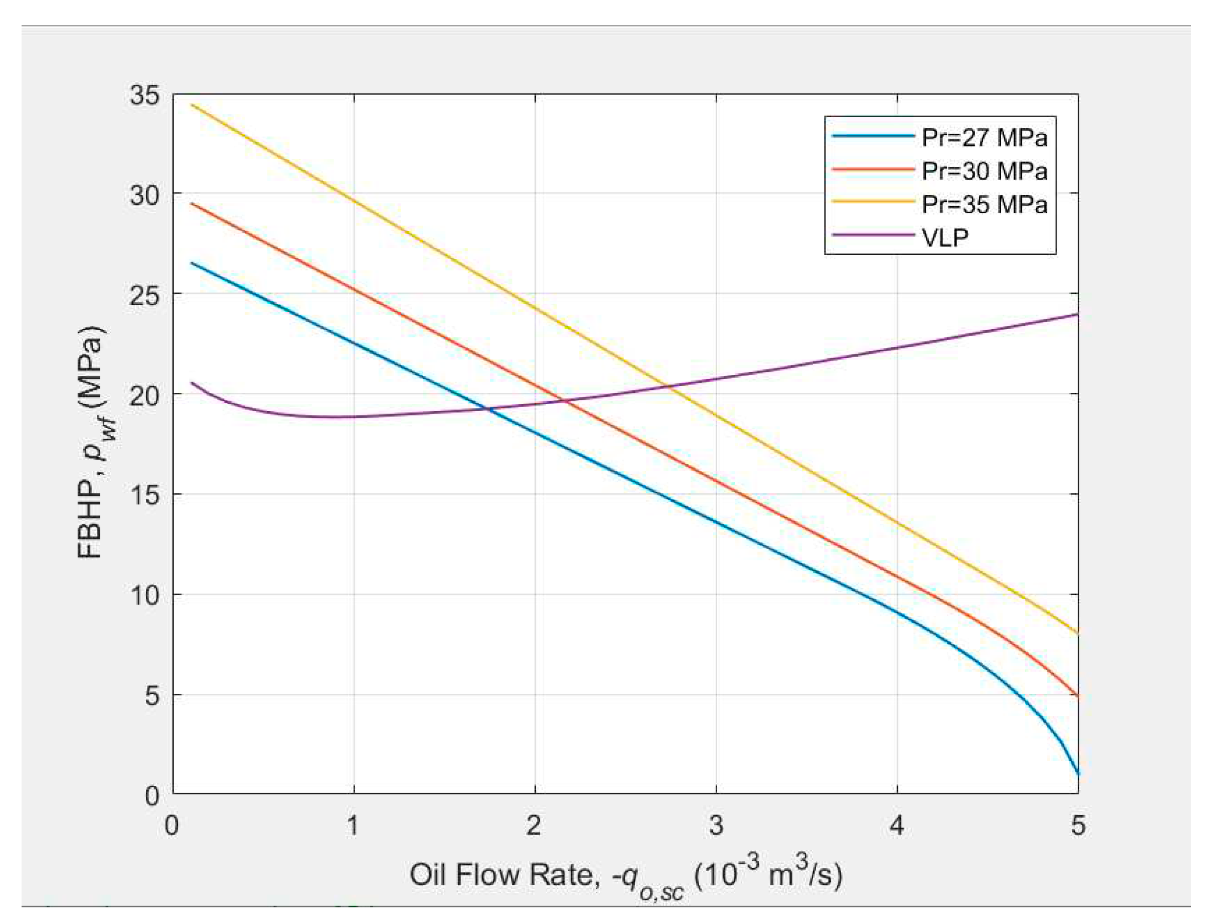

Table 1.
Optimized parameters in the drift flux model (Shi et al. 2005a).
| d | C0,bub | a1 | a2 | m0 | n1 | n2 | |
| >0.1 m | 1 | 1 | 0.06 | 0.21 | 1.85 | 0.21 | 0.95 |
| <0.1 m | 1.2 | 0.6 | 0.06 | 0.12 | 1.27 | 0.24 | 1.08 |
Table 2.
Parameters used for the multiphase flow calculation (Jansen, 2017).
| Parameter | Symbol | SI unit | Field units | ||
| Tubing diameter | d | 62.3×10⁻³ | m | 2.453 | in |
| Roughness | e | 30×10-6 | m | 0.0012 | in |
| Water cut | fw | 0.2 | - | 0.2 | - |
| FTHP | ptf | 0.5×10⁶ | Pa | 72.5 | psi |
| Gas/oil ratio | Rgo | 50 | m3/m3 | 281 | scf/STB |
| FTHT | Ttf | 30 | °C | 86 | °F |
| FBHT | Twf | 120 | °C | 248 | °F |
| Well depth | Ztot | 3000 | m | 9843 | ft |
| Inclination | α | 1.0472 | rad | 60 | ° |
| Gas viscosity | µg | Carr et al. (1954) | Pa·s | mPa·s | |
| Oil viscosity | µo | Beggs and Robinson (1975) | Pa·s | mPa·s | |
| Water viscosity | µw | 0.35×10⁻³ | Pa·s | 0.35 | mPa·s |
| Gas density/gravity | ρg,sc/γg | 0.95 | kg/m3 | 0.77 | - |
| Oil density/gravity | ρo,sc/γAPI | 850 | kg/m3 | 35 | °API |
| Water density | ρw,sc | 1050 | kg/m3 | 65.5 | lbm/ft3 |
| Gas/oil IFT | σgo | 0.008 | N/m | 8 | dynes/cm |
| Gas/water IFT | σgo | 0.04 | N/m | 40 | dynes/cm |
Table 3.
Parameters used for IPR calculation (Jansen, 2017).
| Parameter | Symbol | SI unit | Field units | ||
| Reservoir height | h | 30 | m | 98.42 | ft |
| Reservoir radius | re | 400 | m | 1312.34 | ft |
| Permeability | k | 1×10-14 | m2 | 10 | mD |
| Forchheimer coeff | β | 0 | 1/m | 0 | 1/in |
| Endpoint gas | krg0 | 0.7 | - | 0.7 | - |
| Endpoint oil | kro0 | 0.9 | - | 0.9 | - |
| Endpoint water | krw0 | 0.5 | - | 0.5 | - |
| Corey gas | ng | 3 | - | 3 | - |
| Corey oil | no | 3 | - | 3 | - |
| Corey water | nw | 3 | - | 3 | - |
| Corey oil/gas | nog | 3 | - | 3 | - |
| Corey oil/water | now | 3 | - | 3 | - |
| Critical gas sat. | Sgc | 0.0 | - | 0.0 | - |
| Critical oil sat. | Soc | 0.1 | - | 0.1 | - |
| Critical water sat. | Swc | 0.15 | - | 0.15 | - |
Disclaimer/Publisher’s Note: The statements, opinions and data contained in all publications are solely those of the individual author(s) and contributor(s) and not of MDPI and/or the editor(s). MDPI and/or the editor(s) disclaim responsibility for any injury to people or property resulting from any ideas, methods, instructions or products referred to in the content. |
© 2023 by the authors. Licensee MDPI, Basel, Switzerland. This article is an open access article distributed under the terms and conditions of the Creative Commons Attribution (CC BY) license (http://creativecommons.org/licenses/by/4.0/).
Copyright: This open access article is published under a Creative Commons CC BY 4.0 license, which permit the free download, distribution, and reuse, provided that the author and preprint are cited in any reuse.


