Methodology for Assessing the Technical Condition and Durability of Bridge Structures

Запропонована методика спрямована на визначення та прогнозування технічного стану елементів мосту, що може слугувати прогресивним інженерним інструментом для оцінки надійності та довговічності. Розроблено на основі фундаментальних досліджень, які узагальнюють досвід вивчення фізико-механічних і фізико-хімічних властивостей матеріалів мостових конструкцій, що експлуатуються в реальних умовах. Теоретичною основою методики є модель надійності та прогнозування залишкового ресурсу елементів мосту на основі теорії Маркова. Розроблена методика призначена для оцінки технічного стану окремих елементів мосту з подальшою комплексною оцінкою всієї конструкції. За показник технічного стану прийнята надійність при експлуатації. Цей кількісний показник надійності в моделі є критерієм для: оцінки рівня безпеки елементів мосту; ранжування елементів мосту за необхідністю для конкретних видів ремонту, реконструкції або заміни; стратегічне планування витрат на ремонт або реконструкцію в умовах обмеженого фінансування; прогнозування залишкового ресурсу елементів. Для застосування розробленої методики запропоновано алгоритм оцінки та прогнозування технічного стану мостів. Було проведено математичний експеримент розробленої методики, який підтвердив адекватність висунутої гіпотези, тобто використання моделі надійності та прогнозування залишкового ресурсу елементів мосту. По-перше, запропоновано триступеневий механізм уточнення технічного стану мосту, суттєво підвищення точності розрахунків. Тому розроблена методика має практичне значення і може слугувати основою для інформаційно-аналітичних систем управління станом мостів.

Keywords:

Subject: Engineering - Civil Engineering

1. Introduction

The assessment of the technical condition of bridges is a crucial aspect of effective operational maintenance management. Inadequate maintenance of bridge elements affects the overall structure’s durability. The performance and operational characteristics of bridges deteriorate over time, and they are constantly subjected to the aggressive influence of the environment (humidity, temperature, wind erosion), mechanical damage during winter maintenance, increased traffic intensity, and higher demands for load capacity [1]. This necessitates continuous monitoring of the state of bridges, as well as forecasting the residual capacity to take preventive actions for structure preservation. Thus, the theoretical approaches to testing bridges with subsequent diagnosis of their technical condition, taking into account the structural state and assessing their overall condition, were analyzed in the study.

In studies [1,2], the experience of managing the condition of bridges based on degradation models using information-analytical bridge management systems has been analyzed. It is emphasized that the accuracy of the decisions made, significantly depends on the model for predicting the bridge’s residual lifetime. The most common types of models used as the basis for bridge management information systems were deterministic orstochastic. However, authors in [3] have determined that mathematical formulations to describe degradation processes often have high complexity, so practical degradation models frequently rely solely on inspection results. Authors in [1,2] also emphasized that these models had inaccuracies in calculating the reliability of structural elements when determining the operational condition of bridges.

Reliability is one of the most important requirements for structures as outlined in the Eurocodes [4]. Therefore, it is crucial to ensure that the parameters of safety level, suitability for operation, and durability correspond to this indicator. In the study [5], a critical overview of models for calculating and predicting the technical condition of bridges based on the reliability parameter is provided. It is emphasized that most models are based on determining reliability for elements with a standard set of constructions and materials. Authors in [5] propose a hybrid calculation model that combines a modified process of fuzzy analytical hierarchy analysis (EA FAHP) and dominant analytical hierarchy process (DAHP). However, the authors note the complexity of calculations using their developed model for practicing engineers.

In the work [5], it is proposed to use a mathematical framework based on fuzzy logic and transition intensity from one state of the bridge to another to determine the technical condition of the bridge. The rating of the bridge condition is achieved by summing the products of all component ratings by their relative importance.

By using degradation models, a deterministic value of the averaged predicted state of the bridge can be obtained. In research and in practice in several countries, deterministic methods of condition assessment are used, such as linear extrapolation, linear, non-linear, and stepwise regression, as well as methods based on degradation curves [6,7]. However, these methods do not take into account historical data on the changes in the condition of bridge elements. Thus, they can only be applied to short-term degradation forecasting [2].

In the contribution [8], the application of stochastic models is investigated, considering the degradation of bridge elements as a probabilistic process accompanied by uncertainty and randomness. The most commonly used stochastic models for predicting the degradation of infrastructure objects are considered to be Markov models, which are used in the majority of information-analytical bridge management systems in various countries [2,9]. It is believed that the advantage of using Markov models is the ability to forecast the condition of a structure based on available information from at least two visual inspections. In other words, these models operate on the assumption that the probability of the future state of the structure depends solely on its current technical condition. The first Markov degradation model in Ukraine was proposed by Prof. A.I. Lantukh-Lyashchenko in 1999 [10]. Subsequently, the model was further developed and improved in works [11,12] and was verified in practical applications as an updated normative model for assessing and predicting the technical condition of bridge elements [13]. In the practices of Slovakia and the Czech Republic, a combined approach based on several models is used in the standards for assessing and predicting the condition of bridges [14].

However, despite the recognition of these models as the most effective for predicting the condition of structures, it is considered that existing information-analytical systems based on these models in various countries have a number of drawbacks [2]. In particular, this includes the failure to account for the overall service life of the bridge in determining the transition probability from one state to the next [15]. Kleiner [16] proposed using probability distributions with increasing failure rates for an indefinite time of the structure being present in each conditional state. This underscores the issue of accelerating the degradation of bridge elements at higher operational states. Thus, there is a problem of determining the probability of transitioning to the next state for bridges of different service lives.

Another issue is the non-uniformity of obtaining actual data from inspections or measurements of technical indicators of bridge elements. In the study [2], it is emphasized that the determined operational state is not an accurate indicator of safety and suitability for use of the structure. Therefore, it is considered impossible to achieve precision in determining the state of the bridge solely based on the data from inspecting its elements.

In the field of bridge engineering, separate developments have been made in models based on the use of artificial intelligence, Bayesian networks (BN), Petri-Net (PN) models, and others. These models were developed as an attempt to overcome some limitations of existing traditional models [2].

Thus, the models and methods for assessing and predicting the technical condition of bridges identified in the studies [1,2,3,4,5,6,7,8,9,10,11,12,13,14,15,16] are not perfect, have limitations in their application, and require refinement. Additionally, the analysis of these studies has shown that adequate results cannot be obtained using traditional models. However, the significant attention of researchers to this problem confirms the relevance of the proposed research direction.

Based on the theory of the process of assessing the technical condition of bridges we develope a methodology for determining the technical condition and durability indefinite in terms of residual lifetime of bridge structures.

2. Materials and Methods

The main goal of inspecting bridge structures is to determine their technical condition and operational mode, as well as to assess their ability to withstand the designed loads, considering any detected defects. The results of the inspection provide conclusions regarding the current state of the bridge, its load-bearing capacity, the parameters of temporary loading, which the structure can withstand. This information is crucial for making decisions about repair or reconstruction.

To formalize the inspection process, Ukrainian regulatory documents [13] consider a bridge structure as a system consisting of seven groups of structural elements: span elements, supports and bearing parts, foundations, roadway elements, approaches, substructure elements and acesssories. The categorization of bridge elements into these groups takes into account their functional characteristics, allowing for the determination of the significance of each element for the subsequent trouble-free operation of the structure. It is worth noting that these groups of elements are subjected to various force factors, have different functions, service life, and influence on the overall structural stability.

The analysis of the inspection materials allows for the assessment of the technical condition of each group of bridge elements, enabling the determination of the operational state of the element group and the bridge structure as a whole. The basis for categorizing a bridge element into a particular operational state is based on data obtained through the analysis of the bridge’s primary technical documentation, operational records, examination of the operational history, detailed inspection of the entire structure and its elements, assessment of material strength at the time of inspection, load-bearing capacity verification, and determination of the actual safety characteristics of the elements, as well as conducting load tests if necessary.

In this research, bridges are considered as systems consisting of seven groups of structural elements. Subsequently, the technical condition of these elements is assessed by classifying them into one of the five accepted operational states (see Table 1). The classification is based on data collected during inspections and is regulated by normative documents (e.g., [13]), including:

Primary technical documentation of the bridge;
Operational documentation data;
Analysis of the operational history;
Detailed inspection data of the entire structure and its elements;
Determination of the actual material strength of the structural elements;
Bridge testing data (if necessary).

According to the requirements of regulatory documents [13], validation calculations of load-bearing capacity are performed to determine the actual safety characteristics of the elements for refining the operational state.

The normative documents contain necessary classification tables, which are based on the assumption that widely used methods and tools are applied for inspections and examinations of bridges in the country. It should be noted that the tables in most countries are open for modernization and are constantly updated. This means that over time, experience will accumulate in inspections using advanced methods, and the tables will be supplemented with corresponding new quantitative and qualitative characteristics of operational states.

The procedure for classifying the state of bridge elements based on inspection results involves correlating defects and damages recorded during inspections with the descriptions of states provided in the degradation tables. Given that reliability (safety characteristic) is defined for each discrete state in the tables, the conclusion regarding the classification of the operational state of the element simultaneously determines its reliability.

Traditionally, three methods are used for predicting the service life of bridges: the coefficient method, the loading function method, and the principle of time segments.

The Coefficient Method, based on initial data, starts with a reference service life of the structure which is subsequently adjusted using coefficients. These coefficients account for factors such as the quality of construction materials, design level, manufacturing quality, internal and external environmental influences, usage of the structure, and maintenance level [17].

The Loading Function Method is formulated as a comparison of two stochastic variables: the influence of loading and the surrounding environment, and the resistance of the structure. By comparing these two values, information about the safety and performance (reliability) of the structure over time can be obtained. In specific cases, coefficients may be expanded. For instance, material quality coefficients may vary based on material grade. This method is used for a rough assessment of the technical state using coefficients.

The next method is the Time Function of Structure Operation. Based on this function, an exponential law is used to determine the operational time of the structure and the degree of its degradation.

The proposed model for predicting the operational state is based on phenomenological classification tables of discrete states and degradation functions. This model relies on four postulates (Figure 1):

The criterion for the technical state of an element is a numerical reliability parameter.
The life cycle of an element in operation is divided into 5 discrete states. Each state is described by a set of quantitative and informal (linguistic) qualitative degradation indicators, characterizing the hierarchy of element failures [18].
The process of element degradation throughout the operational life cycle is described by a discrete model of a continuous-time Markov process.
The time of transition between discrete states occurs at random time points.

3. Results

Based on the conducted research, an algorithm for assessing and predicting the technical condition of equipment was developed (Figure 2).

The algorithm for assessing and predicting the technical condition consists of the following main steps:

Step 1: Classification of the condition of bridge elements based on inspection and/or testing results using classification tables.

The procedure for classifying the operational condition of the bridge elements based on inspection involves correlating characteristic defects, damages, and other degradation indicators recorded during inspections and tests with the description of their degradation process provided in the classification tables of the regulatory document [13]. Based on this correlation, each element is assigned to one of the five operational states (Table 1). In cases where the wear level of an element or the state of its degradation is not specified in the information tables, the expert classifies the state using the general description of operational states of the structure. This procedure is notably subjective and heavily reliant on the expertise of the inspector conducting the survey.

Step 2: Classification of the state of bridge superstructures based on the calculation of their load-bearing capacity.

Determining load-bearing capacity is a mandatory regulatory procedure aimed at refining the classification of the operational condition of an element. Load-bearing capacity is determined with respect to temporary moving loads that were applicable at the time of design. The determination of load-bearing capacity of superstructures is performed based on the actual dimensions of structural elements, mechanical properties of materials, and a description of observed defects recorded during inspection.

In cases where the operational condition classified by load-bearing capacity is lower than what was obtained in Step 1, this condition should be conclusively accepted.

Step 3: Classification of the state of bridge superstructures based on the results of analytical calculation of their real-time safety characteristics. This calculation serves to refine the classification of the condition.

The initial data for determining safety characteristics include inspection data with specified mechanical characteristics of materials, quantitative indicators of degradation of their cross-section, aggregated values of resistance, and loads. Parameters reflecting the probabilistic nature of stress-strain state factors of the element are coefficients of variation of strength characteristics of materials and temporary moving load. These data are independent of the current state of the bridge element and are provided in regulatory documents.

Step 4: Prediction of the remaining service life of bridge elements.

The period of trouble-free operation of the bridge is predicted in accordance with the recommendations of regulatory documents. The degradation model of the element, i.e., the transition from one operational state to another, is described as a discrete-state Markov process with continuous time. The initial data for determining the remaining service life are the reliability of the element, the time elapsed from the start of operation to the time of inspection, and the failure intensity. These data are obtained based on inspections, load-bearing capacity verification calculations, real-time safety characteristic calculations, and operational state classification.

The failure intensity for the element is found from the degradation equation as its solution under known initial conditions: the reliability of the element in the i-th operational state obtained from the classification table of operational states, and the time elapsed from the start of operation of the element to the moment of classification of its operational state. The remaining service life of the structure as a whole (prediction of the period of trouble-free operation) is estimated based on the lowest of the remaining service life indicators of the superstructures, supports, and foundations.

Step 5: Assignment of operational measures for the considered elements is carried out using normative tables. For all discrete states, the level of wear of the element (in %) and the necessary regulatory operational measures for each state are determined.

Step 6: For integral assessment of the technical condition of the structure, two indicators are introduced: operational assessment of the bridge as a whole based on basic classification and formalized expert assessment of the technical condition of the entire structure.

The operational assessment of the bridge as a whole is a comprehensive characteristic of the operational suitability of the structure in the state of its non-bearing elements. The operational condition of the bridge is classified as the lowest among the indicators of the operational condition of its three main bearing elements: superstructure, supports, and foundation.

The expert operational assessment (rating) of the bridge as a whole is an integral comprehensive characteristic of the operational suitability of the bridge, determined by the state of all seven of its elements. For this purpose, a 100-point scale of dimensionless coefficients is used.

Formalized expert assessment (rating) is used for:

Ranking structures within a specific road network, with the need for repair or reconstruction.
Planning expenditures for repairs, reconstruction, or the construction of new structures.
Establishing the maintenance regime of the structure.
Determining the timing and types of repairs.
Assigning parameters for strengthening and widening of the roadway.
Making decisions regarding the necessity and feasibility of replacement, reconstruction, or major repairs.

Depending on the rating of the structure, the need for corresponding operational measures is determined.

Step 7: Assignment of operational measures for the bridge as a whole.

This final formalized stage of the procedure involves making the necessary operational decisions in accordance with the recommendations of regulatory documents.

In the methodology, it is assumed that reliability calculation is carried out on the theoretical basis [18]. In this case, the reliability of the structure (or its element) is the probability that the value of the generalized strength reserve will be positive, i.e.,

P = P_{r o b} (S > 0),

(1)

where P is the reliability of the structure and S is the strength reserve. The strength reserve is defined as the difference between the generalized resistance of the element and the generalized load:

S = R - Q,

(2)

where R denotes the generalized resistance of the element and Q is the generalized load on the element. In most practical tasks, the generalized resistance of the element and the load are considered random variables following a normal distribution. Therefore, according to [18], the strength reserve will also be a random variable, following a normal distribution (Figure 3):

μ_{S} = μ_{R} - μ_{Q}; σ_{S} = \sqrt{σ_{R}^{2} + σ_{Q}^{2}}

(3)

where

μ_{R}

μ_{Q}

denote the mathematical expectations of the generalized resistance and load respectively and

σ_{R}

σ_{Q}

are the standard deviations of the resistance and load distributions respectively.

Then the probability of structural failure is determined by:

V = P_{rob} (S < 0) = P_{S} (0) = \int_{- \infty}^{0} p_{S} d S,

(4)

where

p_{S}

is the probability function of strength reserve. Then, considering that

P + V = 1

, and

p_{S}

follows a normal distribution, we obtain [18]:

P = \frac{1}{2} + Φ (β),

(5)

where function

ϕ (x)

is the Gaussian probability integral. Safety characteristic

β

is determined by the formula

β = \frac{μ_{S}}{σ_{S}} .

(6)

As seen from Figure 1, the parameter

β

determines the number of standard deviations within the interval from

S = 0

S = μ_{S}

. By considering (3) and (6), the safety characteristic can be expressed as

β = \frac{μ_{R} - μ_{Q}}{\sqrt{σ_{R}^{2} + σ_{Q}^{2}}} .

(7)

Let’s introduce a deterministic value called the factor of margin

γ = \frac{μ_{R}}{μ_{Q}} .

(8)

Then, Equation (7) takes the form

β = \frac{γ - 1}{\sqrt{ν_{Q}^{2} + γ^{2} ν_{R}^{2}}},

(9)

where

ν_{R} = \frac{σ_{R}}{μ_{R}}

and

ν_{Q} = \frac{σ_{Q}}{μ_{Q}}

are coefficients of variation for the variables R and Q respectively.

The formula for determining the safety characteristic (9) has an advantage over formula (7) because the coefficients of variation can be estimated even with insufficient statistical information regarding the structural resistance and loading.

In a separate case, when the strength of the structure can be considered a deterministic quantity

(ν_{R} = 0)

, formula (9) takes the form:

β = \frac{γ - 1}{ν_{Q}} .

(10)

Thus, it has been shown that the reliability of the structure is uniquely expressed through the safety characteristic. It is proposed that bridge structures are divided into 5 states based on their operational condition (Table 1).

This number of states, in our view, is optimal. Each state corresponds to its own interval of

β

, and therefore the reliability calculated from (5). In most cases, the design value of the safety characteristic should be within the range of

β = 3.8 - 4.5

, which corresponds to the reliability interval of

P = (0.999928 - 0.999997)

. This reliability interval for bridge structures is quite sufficient. However, as experience shows, high design (or initial) reliability does not guarantee that the structure will operate without failure for the specified period required by regulatory requirements. In other words, initial reliability does not guarantee the specified service life. This is due to many factors, including the rate of material degradation, the quality of work executed, possible design flaws, and so on. Determining the time (or remaining capacity) by which the structure will transition to the 5-th (inoperative) state is the second part of the reliability theory problem.

According to the multiplication theorem, a complex event

P (t)

can be represented as the product:

P (t) = P_{0} \cdot P_{t} (t),

(11)

where

P_{0}

is the initial or design reliability at the start of structure operation

(t = 0)

is determined by formula (5),

P_{t} (t)

is the probability of failure-free operation of the structure until time

t > 0

. It is assumedthat when

t = 0

P_{t} (t) = 1 .

(12)

In other words, the function

P_{t} (t)

can be considered as the reliability of the structure at time

t > 0

, provided that its initial reliability (12) equals one.

Currently, there is no universally accepted model for determining reliability as a function of time. As one of the possible options, the research suggests determining

P_{t} (t)

using the Markov model of damage accumulation.

The failure rate function

λ_{f r}

(fail rate) is one of the most important parameters in reliability theory [18], which is associated with the reliability by the relationship:

λ_{f r} (t) = - \frac{1}{P} \frac{d P}{d t} .

(13)

The physical meaning of the function

λ_{f r} (t)

is that it equals the probability of failure within the time interval

(t, t + d t)

given that the structure has been operating without failure up to time t. At the beginning of the structure’s operation, when its reliability is close to one, taking into account (4) can be expressed as:

λ_{f r} (t) \approx - \frac{d P}{d t} = \frac{d V}{d t} .

(14)

That’s why the function

λ_{f r} (t)

is sometimes referred to as the degradation rate (reliability reduction rate) of the structure.

With the consideration of (11), the dependency (13) can be expressed as:

λ_{f r} (t) = - \frac{1}{P_{t}} \frac{d P_{t}}{d t} .

(15)

As we can see from (15), the failure intensity function does not depend on the initial reliability of the structure. If we assume that

λ_{f r} (t)

does not depend on time

(λ_{f r} (t) = λ_{C} = c o n s t)

, then from (15) we obtain the well-known exponential degradation law:

P_{t} (t) = e^{- λ_{C} t} .

(16)

This law is widely used for solving many reliability theory problems, particularly for various functional-purpose and bridge structures.

It’s worth noting that, based on practical operating experience, the failure intensity function cannot be considered constant throughout the entire life cycle. This is due to the significant role that metal and concrete corrosion plays in the degradation process of bridge structures. As of today, steel and reinforced concrete are the main materials used for bridge structures. At the beginning of a structure’s operation, when the reinforcement is covered with a protective layer of concrete, corrosion practically does not develop. Therefore, the rate of degradation, and hence the failure intensity function, will approach zero at this stage. With the development of corrosion processes, the derivative of the failure intensity function begins to increase, reliability decreases accordingly, and thus,

λ_{f r} (t)

increases quite quickly. Therefore, the application of the exponential degradation law (16) can lead to significant errors in determining the degradation process of the structure, which in turn will lead to errors in determining the remaining resource.

Therefore, to determine the probability of failure of a structure that would correspond more to real operating conditions, the authors propose a method based on a continuous-time discrete-state Markov model.

According to this model, the transition time from one state to another occurs at random points in time. The operational states (Table 1) that a structure may be in are adopted as the states of the Markov chain. Let’s consider the process graph in the form of Figure 4, where

λ_{i j}

is the density of the flow of random events (transition intensity) that transfers the system from state i to state j.

In the general case, transitions between states can be arbitrary. For example, if a transition from state 3 to state 1 is possible (due to repairs), the corresponding parameter

λ_{i j} \neq 0

It is important to emphasize that despite similar notations, the quantities

λ_{i j}

and

λ_{f r} (t)

are different functions with different physical meanings.

As known [18], a continuous-time Markov process is described by the Kolmogorov differential equations system, which in the considered case will have the form:

\{\begin{matrix} \frac{d p_{1}}{d t} & = - λ_{12} p_{1}; \\ \frac{d p_{2}}{d t} & = - λ_{23} p_{2} + λ_{12} p_{1}; \\ \frac{d p_{3}}{d t} & = - λ_{34} p_{3} + λ_{23} p_{2}; \\ \frac{d p_{4}}{d t} & = - λ_{45} p_{4} + λ_{34} p_{3}; \\ \frac{d p_{5}}{d t} & = λ_{45} p_{4} . \end{matrix}

(17)

In matrix form, this system takes the following shape:

\frac{d p}{d t} = A p,

(18)

where

p = {[p_{1}, p_{2}, p_{3}, p_{4}, p_{5}]}^{T}

is a column vector,

p_{i} (t)

is the probability of the system being in the i-th state and

A

is theflow density matrix. For the given system (17) matrix

A

is of the form:

A = ∥\begin{matrix} - λ_{12} & 0 & 0 & 0 & 0 \\ λ_{12} & - λ_{23} & 0 & 0 & 0 \\ 0 & λ_{23} & - λ_{34} & 0 & 0 \\ 0 & 0 & λ_{34} & - λ_{45} & 0 \\ 0 & 0 & 0 & λ_{45} & 0 \end{matrix}∥ .

(19)

Since the system can only be in one of the five states, we can express it as:

\sum_{i = 1}^{5} p_{i} (t) = 1 .

(20)

Condition (20) is the normalization condition for (17).

The initial conditions for integrating (17) characterize the state of the system at time

t = 0

p_{1} (0) & = 1, p_{2} (0) & = p_{3} (0) = p_{4} (0) = p_{5} (0) = 0 .

(21)

If we consider the coefficients

λ_{i j}

to be independent of time, then (17) represents a system of ordinary differential equations of the first order with constant coefficients.

The solution to the system (17) for the case of a homogeneous Markov process with equal coefficients

λ_{i j} = λ = c o n s t

can be obtained using the method of undetermined coefficients [18].

We can write the characteristic equation of the system (17) as:

\det ∥ A - k E ∥ = 0,

(22)

where

E

is a 5thorder identity matrix and k is the characteristic number.

Taking into account (19), the characteristic Equation (22) takes the form:

k {(k + λ)}^{4} = 0 .

(23)

The roots of Equation (23) are the numbers

k = 0

with multiplicity 1 and

k = - λ

with multiplicity 4. Therefore, the vector of fundamental solutions

q = {[q_{1}, q_{2}, q_{3}, q_{4}, q_{5}]}^{T}

will have the form:

q = {[1, e^{- λ t}, t e^{- λ t}, t^{2} e^{- λ t}, t^{3} e^{- λ t}]}^{T} .

(24)

According to the method of undetermined coefficients, we seek the solution of the system (17) in the form:

p_{j} (t) = \sum_{i = 1}^{5} C_{i j} q_{i},

(25)

where

C_{i j}

the constants (undetermined coefficients) are determined from the initial conditions (21).

Thus, the solution of the system (17) takes the form:

\{\begin{matrix} p_{1} (t) = e^{- λ t}, \\ p_{2} (t) = λ t e^{- λ t}, \\ p_{3} (t) = \frac{λ^{2} t^{2}}{2} e^{- λ t}, \\ p_{4} (t) = \frac{λ^{3} t^{3}}{6} e^{- λ t}, \\ p_{5} (t) = 1 - (1 + λ t + \frac{λ^{2} t^{2}}{2} + \frac{λ^{3} t^{3}}{6}) e^{- λ t} . \end{matrix}

(26)

It’s easy to verify that the functions (26) arethe solution of the system (17), which satisfy initial conditions (21), and normalization conditions (20).

The fifth state is a final state (the structure is in a non-operational state), so the probability of the structure being in a given state will be the sought reliability.

P_{t} (t) = 1 - p_{5} (t) = (1 + λ t + \frac{λ^{2} t^{2}}{2} + \frac{λ^{3} t^{3}}{6}) e^{λ t} .

(27)

Taking into account (27), the failure intensity function (13) can be expressed as:

λ_{f r} = \frac{λ^{4} t^{3}}{6 + 6 λ t + 3 λ^{2} t^{2} + λ^{3} t^{3}} .

(28)

Thus, the developed methodology allows for determining the technical condition of individual bridge elements, followed by a general assessment of the entire structure as a whole.

4. Discussion

Let’s conduct a numerical experiment to determine the probability function of the bridge being in the 5th state for failure intensities of

λ = 0.02

per year and

λ = 0.0128

per year (Figure 5a-b).

As we can see from the provided graphs, the reliability of the structure remains practically constant in the initial stage of its operation (10-15 years). After the initial stage, depending on the value of

λ

(

λ = 0.02

per year and

λ = 0.0128

per year), degradation processes start to develop much faster.

Given the known initial reliability of the structure, the analytical relationship (27) allows us to determine the remaining service life, i.e., the time of operation of the structure before it transitions to the 5th (non-operational) state. In this critical state, the reliability of the structure will be

P_{c} r = P (t) = 0.958351

(see Table 1).

To determine the remaining service life of the structure, the initial (design) reliability value, as practical experience shows, is very close to one. Therefore, we will consider that Equation (11) can be replaced with an approximate equality:

P (t) \approx P_{t} (t) .

(29)

Note that this constraint is not significant and does not alter the calculation algorithm.

To determine the remaining service life, it is convenient to express relationship (27) as a function of the parameter:

α = λ t .

(30)

Then, considering (29), we can write:

P (α) = (1 + α + \frac{α^{2}}{2} + \frac{α^{3}}{6}) e^{- α} .

(31)

The graph of function (31) is presented in Figure 6, where the horizontal lines

P = c o n s t

represent the reliability of the structure corresponding to its state according to Table 1.

The point of intersection of the line

P_{c r} = P (t) = 0.958351

with the curve (31) determines the maximum or critical value of the parameter

α_{c r}

. Then, with the known intensity value

λ

, we can determine the service life of the structure T as:

T = \frac{α_{cr}}{λ} .

(32)

From the provided graph, we determine that

α_{c r} \approx 1.28

. If the design service life of the bridge is

T = 100

years, then from Equation (32), we obtain the intensity value

λ = λ_{0} = 0.0128

. This intensity corresponds to a service life of 100 years and can be referred to as the design intensity of transitions between states that the structure may be in. In reality, the value of

λ

can be both greater and smaller than

λ_{0}

To determine the value of

λ

, it is necessary at a certain stage of the bridge’s operation

t = t_{e}

to conduct an inspection, as a result of which the corresponding reliability of the structure

P_{e}

will be determined. Based on the inspection results, the safety characteristic

β_{e}

that the structure has at the moment

t = t_{e}

is determined.

Using the value of reliability

P_{e}

, obtained either from the graph (Figure 6) or by using appropriate programs for finding roots of functions (31), we determine the parameter

α_{e}

and the intensity value

λ

, which is equal to:

λ = \frac{α_{e}}{t_{e}} .

(33)

Thus, the remaining service life of the structure, taking into account (32) and (33), will be equal to:

Δ T = T - t_{e} = (\frac{α_{k r}}{α_{e}} - 1) t_{e} .

(34)

If, as a result of the inspection, only the operational state of the structure is determined, then

P_{e}

is chosen from among the average reliability values for that particular state. This, of course, reduces the accuracy of forecasting the remaining service life, but can be used with insufficient information during the inspection of the structure.

It is important to emphasize that since the parameter

λ

characterizes the degradation process, the inspection time for its accurate determination should be no less than 10-15 years.

5. Conclusions

One of the key parameters in bridge management systems is the remaining service life of the structure, which represents the predicted period of its trouble-free operation. The behavior of a bridge depends on many factors, most of which have a random nature. Therefore, it is logical that degradation models of bridges in most countries are stochastic. One such model is the Markov model of damage accumulation. A significant advantage of the Markov model is that the future behavior of the structure depends only on its present state (known as the memoryless property). This enables the prediction of the remaining service life based on the results of the inspection at the current moment in time.

In many European Union countries, a discrete-time Markov model is applied, assuming that transitions from one state to another can only occur at discrete points in time. In Ukraine, a continuous-time Markov model is currently used. According to this model, transitions between states can occur at arbitrary, random points in time. The corresponding system of differential equations (Kolmogorov equations) was derived based on the Markov model with discrete states and continuous time. The analytical solution of the system of equations using the method of undetermined coefficients allowed for the formalization of the reliability function of the structure and the failure intensity function. As a result, a reliability graph was constructed, providing a straightforward algorithm for determining the remaining service life of the structure based on the conducted inspection of the bridge’s condition.

From the provided reliability and failure intensity function graphs, it can be concluded that for a certain period (approximately 10-20 years), the reliability of the structure remains practically unchanged. This indicates that during this time, degradation processes in the structure hardly occur, if disregarding unexpected events. Therefore, the parameter

λ

, which characterizes the deterioration of the structure’s condition, and the corresponding remaining service life can be accurately determined only after 20 years of operation. An advantage of such a model is that the reliability function of the system can be obtained in analytical form, greatly simplifying the algorithm for determining the remaining service life.

Author Contributions

Conceptualization, Kostiantyn Medvedev, Anna Kharchenko, Vitalii Tsybulskyi and Anzhelika Stakhova; methodology, Kostiantyn Medvedev and YuriiYevseichyk; validation, Anzhelika Stakhova and Adrián Bekö; formal analysis, Kostiantyn Medvedev and Yurii Yevseichyk; investigation, Kostiantyn Medvedev, Anna Kharchenko, Anzhelika Stakhova, Vitalii Tsybulskyi and Adrián Bekö; resources, Kostiantyn Medvedev and Vitalii Tsybulskyi; data curation, Kostiantyn Medvedev, Anna Kharchenko, Anzhelika Stakhova, Vitalii Tsybulskyi and Adrián Bekö; writing—original draft preparation, Kostiantyn Medvedev, Anna Kharchenko and Vitalii Tsybulskyi; writing—review and editing, Anzhelika Stakhova and Adrián Bekö; visualization, Anna Kharchenko and Vitalii Tsybulskyi; supervision, Kostiantyn Medvedev and Anna Kharchenko; project administration, Anzhelika Stakhova; funding acquisition, Anzhelika Stakhova and Adrián Bekö. All authors have read and agreed to the published version of the manuscript.

Funding

Funded by the EU NextGenerationEU through the Recovery and Resilience Plan for Slovakia under the project No. 09I03-03-V01-00104

Institutional Review Board Statement

Not applicable

Data Availability Statement

Data sharing not applicable. No new data were created or analyzed in this study. Data sharing is not applicable to this article.

Acknowledgments

We also gratefully acknowledge the financial support by the VEGA Grant Agency of the Slovak Republic, grant number 1/0230/22.

Conflicts of Interest

The authors declare no conflict of interest.

References

Folić, R., Partov, D. Comparative analysis of some bridge management systems. Građevinski Materijali I Konstrukcije 2020, 63(3), 21–35.
Santamaria, M.; Fernandes, J.; Matos, J. C. Overview on performance predictive models–Application to Bridge Management Systems. In Proceedings of IABSE Symposium 2019 Guimaraes, Guimaräes, Portugal, 27-29 March 2019.
Sánchez-Silva, M; Klutke, G-A. Reliability and life-cycle analysis of deteriorating systems; Publisher: Springer International Publishing, Switzerland, 2016.
Koteš, P., Strieška, M., Bahleda, F., Bujňáková, P. Prediction of RC bridge member resistance decreasing in time under various conditions in Slovakia. Materials 2020, 13(5), 1125. [CrossRef]
Fabianowski, D., Jakiel, P., Stemplewski, S. Development of artificial neural network for condition assessment of bridges based on hybrid decision making method–Feasibility study Expert systems with applications 2021, 168, 114271. [CrossRef]
Hatami A, Morcous G. Reliability and life-cycle analysis of deteriorating systems; Publisher: Nebraska Transportation Center, 2011.
Zayed, TM, Chang, L-M, Fricker, JD. Statewide performance function for steel bridge protection systems. Journal of performance of constructed facilities 2002, 16(2), 46–54. [CrossRef]
Biondini, F, Frangopol, DM. Life-cycle performance of deteriorating structural systems under uncertainty. Journal of Structural Engineering 2016, 16(2), F4016001. [CrossRef]
Rogulj, K., KilićPamuković, J., Jajac, N. Knowledge-based fuzzy expert system to the condition assessment of historic road bridges. Applied Sciences 2021, 11(3), 1021. [CrossRef]
Lantukh-Lyashchenko, A. I. Estimation of the reliability of the structure according to the Markov random process model with discrete states (in Ukraine). Collection Automobile Roads and Road Construction 1999, 57, 183–188.
Bashkevych, I. V., Yevseychyk, Y. B., Medvedev, K. V., Yanchuk, L. L. Determining the failure intensity function based on the Markov process (in Ukraine). Automobile Roads and Road Construction 2021, 109, 79–87.
Bashkevych, I. V., Yevseichyk, Y. B., Medvediev, K. V., Fal, A. E., Yanchuk, L. L. Analytical model expert assessment condition of bridges. Automobile roads and road construction 2022, 112, 154–162.
DSTU 9181:2022 Guidelines for the assessment and prediction of the technical condition of highway bridges (in Ukraine); Ministry of Regional Development of Ukraine: Kyiv, Ukraine, 2022.
Slovak Road Administration. Available online: https://www.ssc.sk/en/activities/road-network-development/bridge-management/extract-of-technological-regulations-for-bridge-management.ssc (accessed on 20 September 2023).
Lounis, Z.; Mirza, M. S. Reliability-based service life prediction of deteriorating concrete structures. In Proceedings of 3rd Int. Conf. on Concrete under Severe Conditions, University of British Columbia, Vancouver, Canada, 18-20 June 2001; Vol. 1, P. 965-972.
Kleiner Y. Scheduling inspection and renewal of large infrastructure assets. Journal of infrastructure systems 2001, 7(4), 136–143. [CrossRef]
Kanin, A., Kharchenko, A., Tsybulskyi, V., Sokolova, N., Shpyh, A. Construction of a simulation model for substantiating the parameters of long-term road maintenance contracts. Eastern-European Journal of Enterprise Technologies 2022, 2(3) 116, 33–42.
Strakhova N. YE., Holubyev V. O., Kovalov P. M., Todirika V. V., Khodun V. M. Operation and reconstruction of bridges (in Ukraine); Transport Academy of Ukraine: Kyiv, Ukraine, 2000.

Figure 1. The Theoretical Basis of the Model for Assessment and Prediction of the Technical State of Bridge Elements.

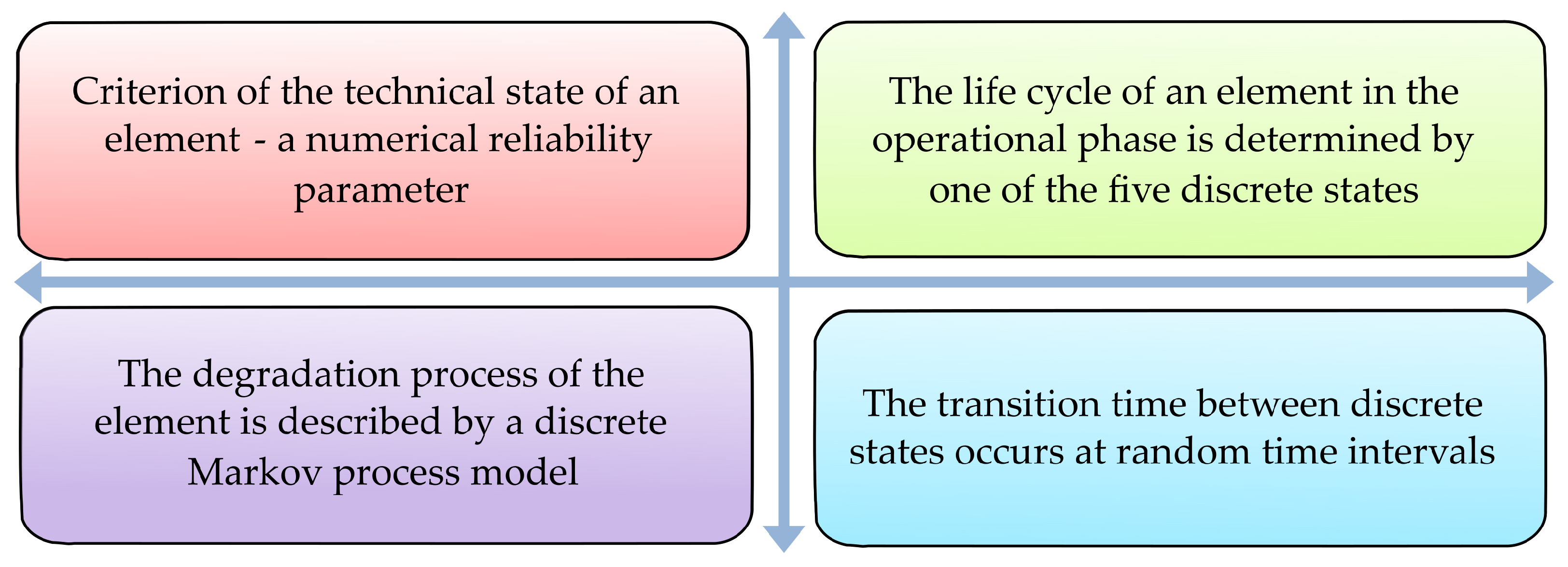
Figure 2. Algorithm for Assessing and Predicting the Technical Condition of the Bridge.

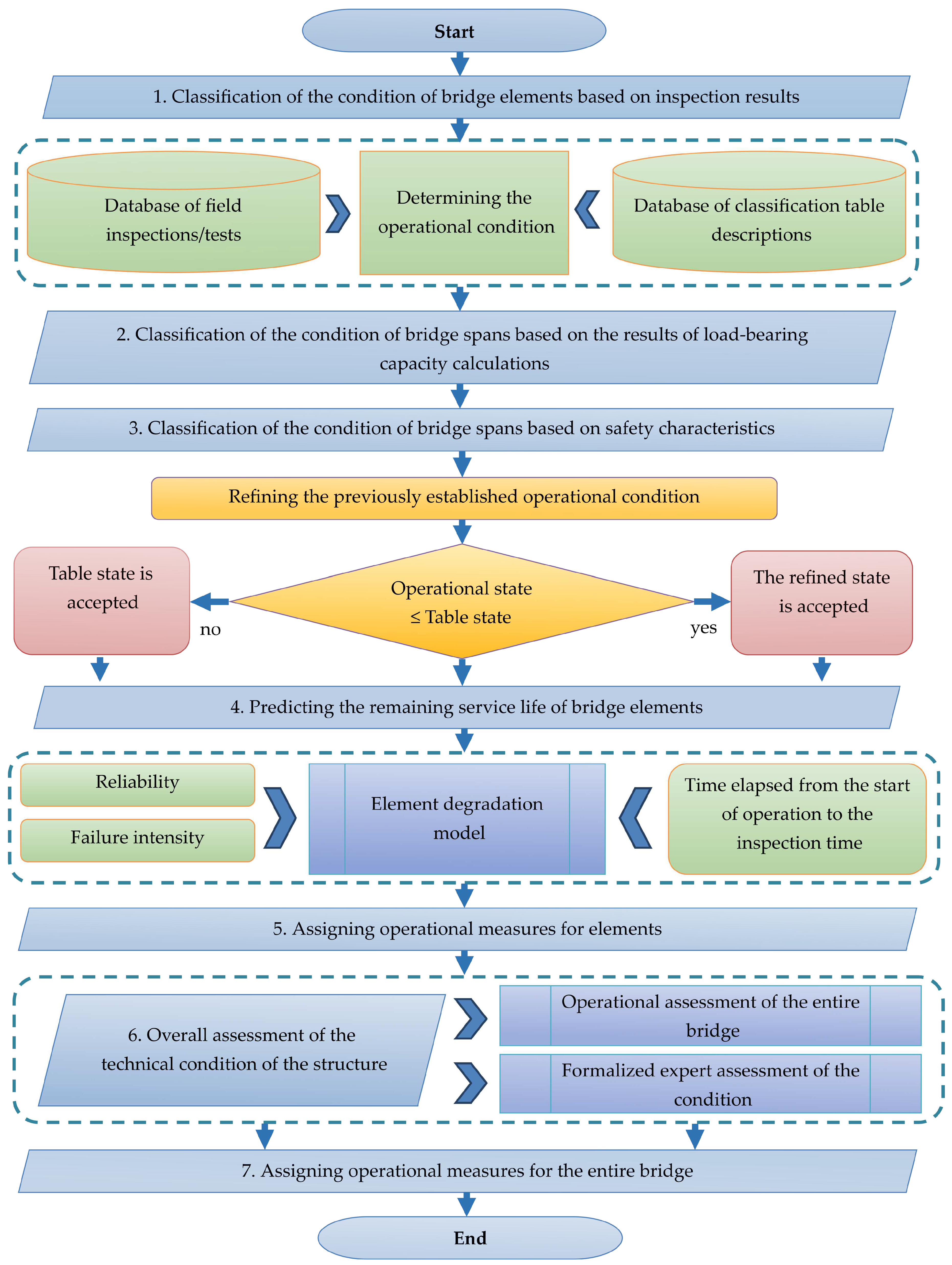
Figure 3. Strength reserve distribution function.

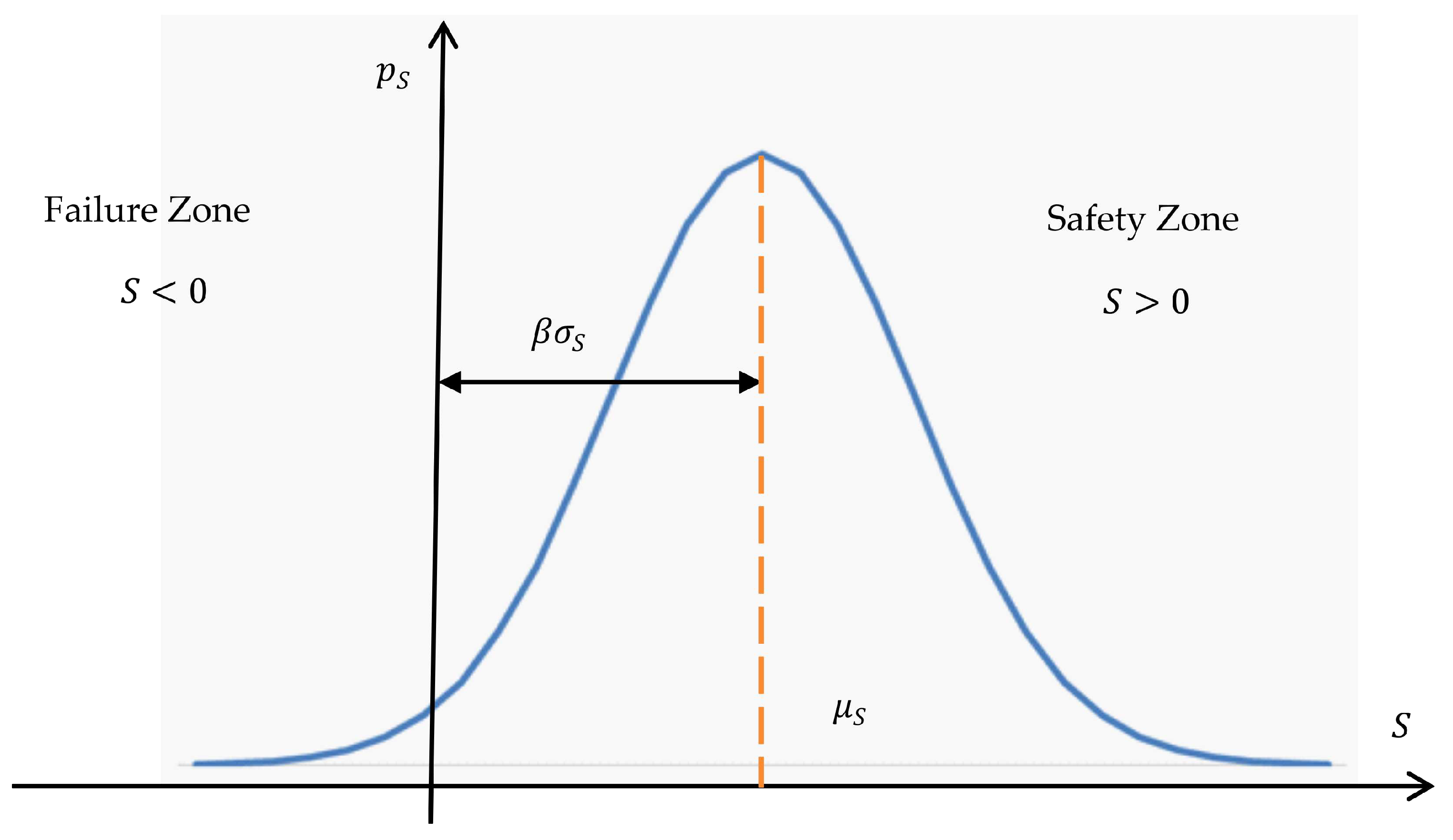
Figure 4. State Transition Graph.

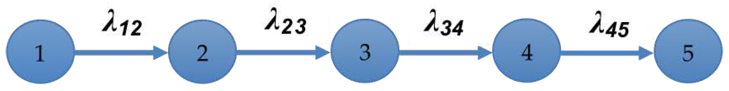
Figure 5. Probability functions (a) and degradation rates (b) for chosen failure intensities.

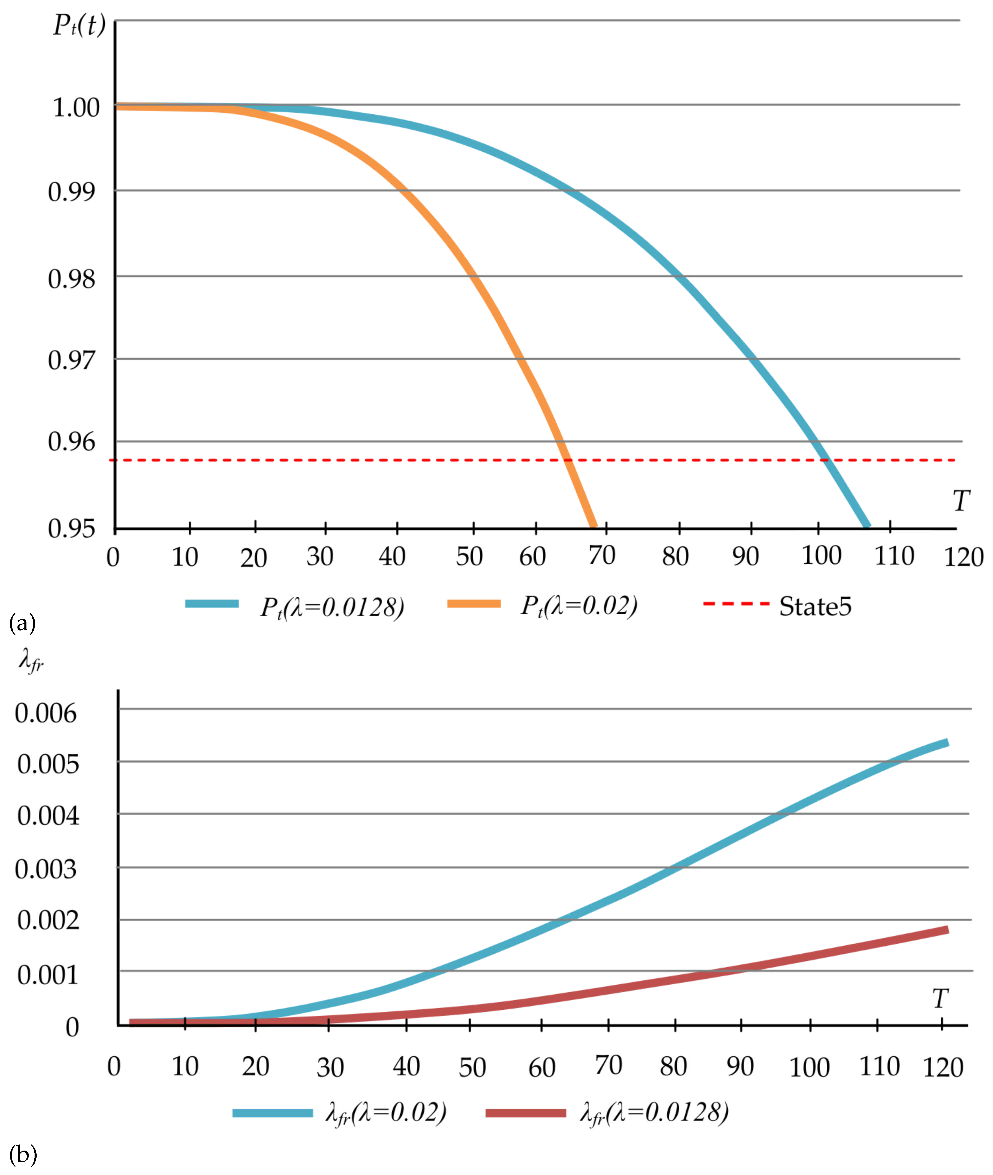
Figure 6. Graph of the reliability dependence on parameter

α

Figure 6. Graph of the reliability dependence on parameter

α

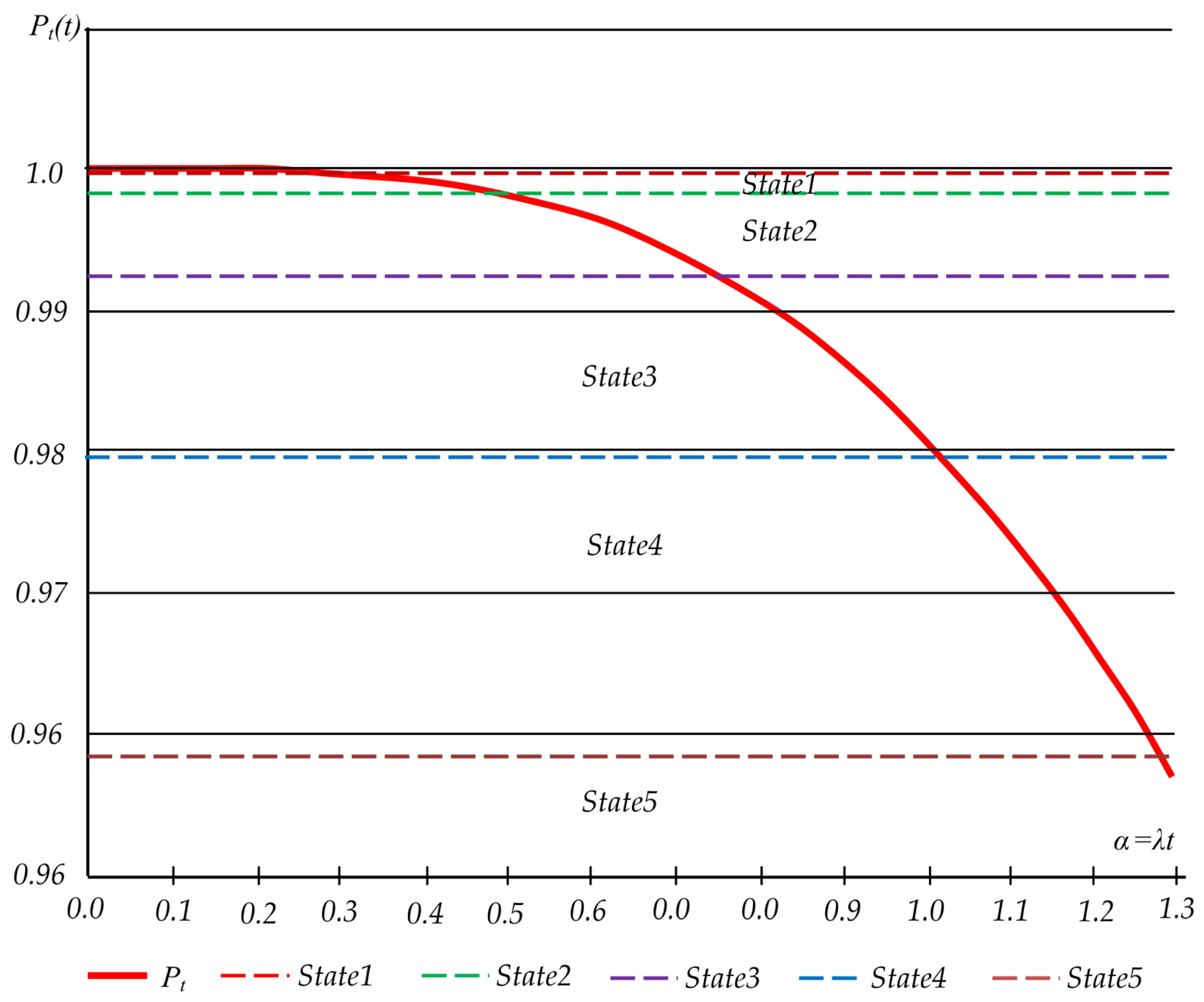
Table 1. Classification of Operational States of Elements.

Operational State	State Name	Reliability (according to the first group of limit states), P	Safety Characteristic, $β$
State 1	Serviceable	0,999844	3,80
State 2	Limited Serviceability	0,998363	2,95
State 3	Operational	0,992461	2,43
State 4	Limited Operational	0,979771	2,05
State 5	Non-Operational	0,958351	1,74

Disclaimer/Publisher’s Note: The statements, opinions and data contained in all publications are solely those of the individual author(s) and contributor(s) and not of MDPI and/or the editor(s). MDPI and/or the editor(s) disclaim responsibility for any injury to people or property resulting from any ideas, methods, instructions or products referred to in the content.

© 2023 by the authors. Licensee MDPI, Basel, Switzerland. This article is an open access article distributed under the terms and conditions of the Creative Commons Attribution (CC BY) license (http://creativecommons.org/licenses/by/4.0/).

Copyright: This open access article is published under a Creative Commons CC BY 4.0 license, which permit the free download, distribution, and reuse, provided that the author and preprint are cited in any reuse.

MDPI Initiatives

Important Links

Choose an area of interest and we will send you notifications of new preprints at your preferred frequency.

Disclaimer

Methodology for Assessing the Technical Condition and Durability of Bridge Structures

Abstract

1. Introduction

2. Materials and Methods

3. Results

4. Discussion

5. Conclusions

Author Contributions

Funding

Institutional Review Board Statement

Data Availability Statement

Acknowledgments

Conflicts of Interest

References

MDPI Initiatives

Important Links

Subscribe