
Submitted:
16 December 2023
Posted:
18 December 2023
You are already at the latest version
Abstract
Squash is a sport where referee decisions are essential to the game. However, referee decisions in squash are very subjective in nature. Disputes, both from the players and the audience, regularly happen because the referee made a controversial call. In this study ,we proposed to automate the referee decision process through machine learning. We trained neural networks to predict squash referee decisions using data from 400 referee decisions acquired through extensive video footage reviewing and labeling. Six positional values were extracted, including the attacking player’s position, the retreating player’s position, the ball’s position in the frame, the ball’s projected first bounce, the ball’s projected second bounce, and the attacking player’s racket head position. We calculated nine additional distance values, such as the distance between players and the distance from the attacking player's racket head to the ball's path. Models were trained on Wolfram Mathematica and Python using these values. The best Wolfram Mathematica model achieved an 86% ± 3.03% accuracy, while the best Python model performed a 0.852 ± 0.051 accuracy (85.2% ± 5.1%). These accuracies surpass 85%, demonstrating near-human performances. Our model has great potential for improvement as it's currently trained with limited data (400 referee decisions) and lacks crucial data points such as time and speed. The performance of our model is almost surely going to improve significantly with a larger training data set. Unlike human referees, machine learning models follow a consistent standard, have unlimited attention spans, and make decisions instantly. If the accuracy is improved in the future, the model can potentially serve as an extra refereeing official for both professional and amateur squash matches. Both the analysis of referee decisions in squash and proposal to automate the process using machine learning is unique to this study.
Keywords:
squash
; refereeing
; machine learning
; neural network
; sport
; referee
1. Introduction
1.1. What is Squash?
Squash is a racket sport played by two people on a four-wall court. The players alternate turns striking the ball, and the goal is to keep the ball in bounds while making the opponent unable to retrieve it before two bounces on the floor. Every shot should hit the front wall before it bounces on the ground for the shot to be deemed as an in-bound shot, while the sidewalls could be used to change the ball’s trajectory before or after the ball has reached the front wall. Squash is considered one of the most physically demanding sports, as the rallies are frequent and last for a long period of time.
1.2. Interferences and Referee Decisions
Because the two players are playing the game in one court, one inevitable aspect of squash is interference. The presence of one player, through inaccurate position or movement, might affect or prevent the shot of another player. For example: player A strikes the ball, but the ball lands back next to player A, and player A is not able to get out of the way (in squash terms, “clear the ball”). In this case, player B would have hit player A if player B attempted to hit the ball. This is one common example of interference. When players are stopped due to interference, the player who is supposed to strike the ball can choose to appeal to the referee for a decision.
In these situations, referees need to make a decision to fairly punish or reward players for the interference that has happened. In squash, there are three possible decisions: Stroke, Yes Let, and No Let. A Stroke for the appealing player awards a point to the player, a Yes Let means the point needs to be replayed, and a No Let for the appealing player awards a point to the other player.
The Professional Squash Association (PSA) defines the decisions and their situations of applications as follows:
“Yes Let decision results in the rally being played again – with the referee deeming that the interference was accidental and both players have made an equal effort to allow play to continue.
No Let decision is where the referee rules against the striker’s appeal and awards a point to the retreating player. In this situation, the referee deemed that the retreating player provided unobstructed access and that interference was minimal, therefore the appealing striker could have played a shot.
Stroke is when the point is awarded to the appealing player. A stroke is awarded when the referee deems the incoming striker is in a position to play a shot, but suffers interference due to the outgoing player not making every effort to clear. ” [1]
The ultimate guidelines for clearing a shot are explained by PSA as follows:
“After playing a shot, players must make every effort to ‘clear the ball’ so that when the ball rebounds from the front wall, the opponent has both
- A)
- a good view of the ball
- B)
- unobstructed access to the ball with the space to make a reasonable swing at the ball
- C)
- the freedom to strike the ball to any part of the entire front wall.
The incoming player must then make every effort to play through minimal interference and complete their shot. A striker who believes that interference has occurred may stop and request a let, at which point the referee must make a ruling, awarding either a ‘Let’, ‘No let’ or ‘Stroke’ [1].
Therefore, in the above-mentioned situation of players A and B, player B would stop and appeal. The correct decision from the referee would be a stroke to player B because player A had obstructed player B’s access to the ball. Therefore, player B would be awarded the point, and the match would continue with the next rally.
1.3. Controversies and Disputes
1.3.1. Regarding the Central Referee
Although all referees should strive for logical, unbiased decisions, the pace of squash and the complexity of professional players’ movements can make some decisions extremely difficult to make. An individual referee’s personal understanding of the game and the referee’s experience in the position could also affect the result. Although PSA has introduced the video review system, many controversies still exist, both between players and referees and from the viewing audiences.
1.3.2. The Video Review System
The video review system consists of a real-time replay system and one video referee. Whenever a player wants to challenge a referee’s decision and, at the same time, has a “review remaining,” the tech crew replays the recording from the past rally from multiple angles, and the video referee makes a decision based on the replay. The new decision can overrule or uphold the previous decision made by the central referee. The replay system allows the video referee to review the interference in slow motion and at various angles, and most of the time the review system can correct the calls. However, the video review can take a long time, including the time needed to retrieve the recordings and the time the video referee needs to fully understand the situation. This significantly disrupts the flow of the game. Therefore, the PSA only allows players one review per game, and if the player successfully reviews a decision, they will get another review. The disruption of the game is still a minor issue. After all, the decision is still made by an isolated individual, and the biases and differences in understanding of the game would also affect the video referee when making those decisions. There are numerous cases in which a controversial call is upheld after being video reviewed, or an even more controversial decision is made after video review.
1.3.3. Controversies and Arguments
PSA struggles with refereeing problems as the sport grows bigger and more popular among people, and the issue has been kept relatively small due to the video review system on the professional tour. However, junior and college squash have been very susceptible to controversial referee decisions as the referee’s words are the final judgment, and there is no way to reverse a referee’s decision. After all, decisions that go against the players’ and the viewers’ common sense undermine both the competing experience and the viewing experience. The PSA has strived to solve this issue by updating referee guidelines and refining the video review system. However, those measures have not been very effective. There still regularly exists dissatisfaction from audiences and arguments between players and referees.
Figure 1.
Example of player interference [2].
Figure 1.
Example of player interference [2].
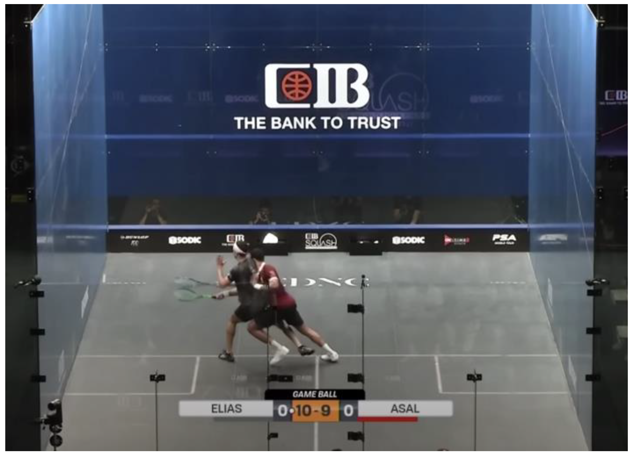
Figure 2.
Player unsatisfied with the decision and. opened the back door to argue with the referee (which would result in conduct warning if the referee does not want the discussion) [2].
Figure 2.
Player unsatisfied with the decision and. opened the back door to argue with the referee (which would result in conduct warning if the referee does not want the discussion) [2].
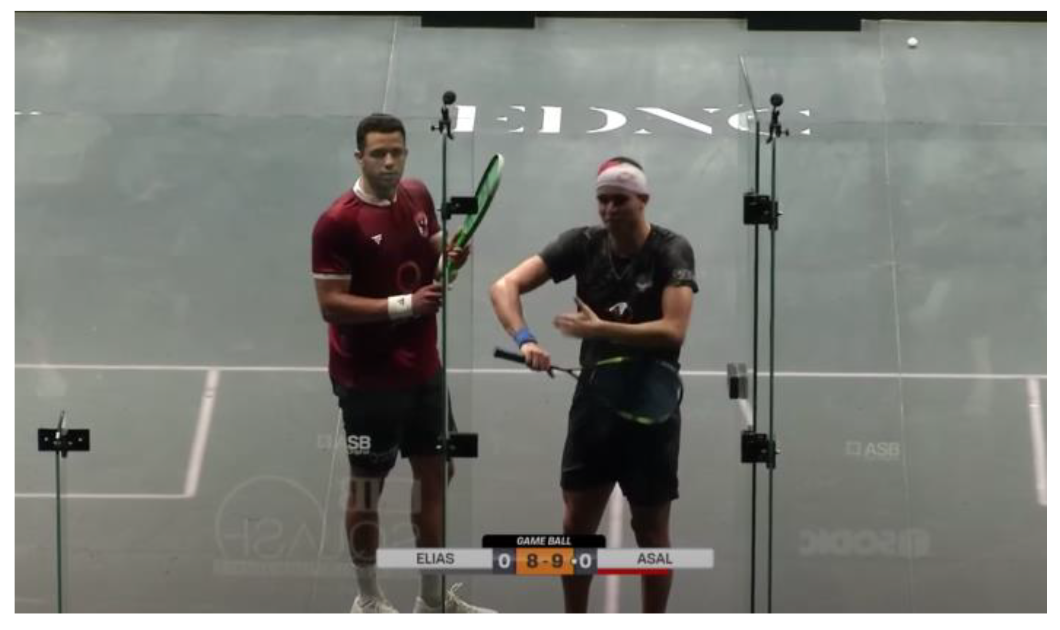
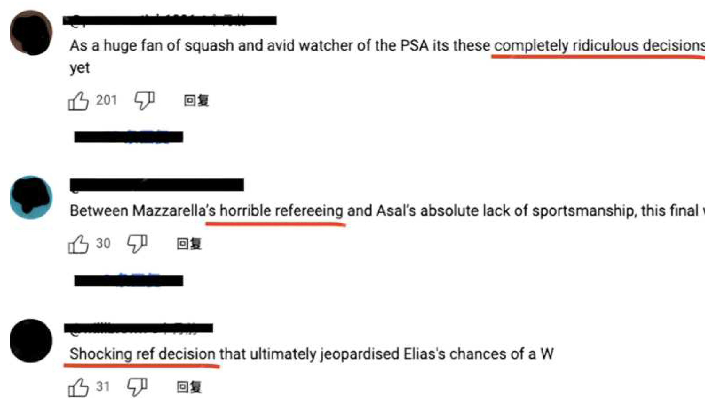
Figure 3.
Audience’s comments under Professional Squash Association’s YouTube channel commenting on their dissatisfaction with the refereeing work [2].
Figure 3.
Audience’s comments under Professional Squash Association’s YouTube channel commenting on their dissatisfaction with the refereeing work [2].
1.4. Machine Learning and Literature Review
One root cause of the controversy is a lack of exact measurement in referee decisions. Usually, referees make decisions based on several evaluations: is there a clear path to the ball? Was the retrieving player blocked from the path to the ball? Could the player have gotten it had there been no interference? Did the player show enough effort to play through the interference? Did the retreating player block the access to the entire front wall? Was it due to safety that the player stopped to appeal? Several crucial ideas exist: clear path, ability to retrieve, effort, blockage, and safety. All referees have different understandings of these concepts, which would result in different decisions. One referee might deem that a player is able to retrieve had there been no interference, but another referee might think the opposite. This disagreement in measures and the fundamental subjectivity underlying these decisions causes the never-ending disputes in squash refereeing.
Machine learning, on the other hand, could eliminate these differences caused by referees’ subjectivity since once the network is trained to have set parameters, the same situation would only result in the same decision. Though it has not specifically been applied to squash refereeing, machine learning has been widely used in sports applications.
For squash specifically, models have been trained to perform player detection and motion analysis [3]. Brumann’s research team investigated more than 250 Human Pose Estimation Convolutional Neural Networks (CNN) and found the five most effective models in the context of motion analysis for squash. The data being used were collected from publicly available squash videos, and Brumann’s team developed their own annotation tool and manually labeled frames and events. Using the labeled data and the trained CNNs, they were able to present heatmaps, which depict the court floor using a color scale and highlight areas according to the relative time for which a player occupied that location during play. Numerous general machine-learning models used for motion detection have also been proposed. In 2013, a motion detection model was proposed utilizing machine learning and data clustering and achieved scene adaptive motion detection [4]. In 2016, a model capable of accurately detecting black and white soccer balls was produced using a series of heuristic region-of-interest identification techniques and supervised machine learning methods [5]. In 2021, a model based on the YOLOv3 object detection model was introduced and addressed the detection of small, fast-moving balls in sport video data [6].
Machine learning has also been applied to the sport of tennis to predict match outcomes [7]. Bayram trained and tested models using advanced machine learning paradigms such as multi-output regression and learning using privileged information on more than 83,000 men’s singles tennis matches between the years 1991 and 2020. The results outperform the existing methods in the literature and the current state-of-the-art models in tennis. In 2018, a tree-based boosting model was proposed to predict biathlon shooting performance [8]. In 2019, a model using the RandomForest algorithm obtained a precision of 0.857 and a recall of 0.750 in soccer match prediction [9]. The model was trained with data acquirable both after the match and during the match play. In 2021, a deep-learning model featuring regression and classification analysis was trained to predict professional basketball players’ future performance and All-Star game selection [10].
In addition to detecting player motion and predicting match results, machine learning has also been utilized to predict shot success in table tennis [11]. In this study, Draschkowitz extracts features like length and direction of strokes from the videos and trained classifiers to predict shot success and failure. After training, these classifiers are capable of predicting the success of strokes for a particular game and player and thus allow players and coaches to adapt to strategies more suitable to specific players.
On the other hand, previous studies have also commented on the inconsistency of referee decisions in competitive sports. In “Influence of crowd noise on soccer refereeing consistency in soccer” [12], researchers investigate the effect of home crowds on referees. They found a significant imbalance of decisions in favor of the home side when crowd noise is present. Although the difference between home and away players for squash is less conceivable compared to soccer, many times the crowd could favor a player over another, which may impose similar effects on the refereeing official. Furthermore, studies have surveyed the empirical literature on the behavior of referees in professional football and other sports and have found that a number of studies have shown that referees favor the home team in football, basketball, or baseball [13]. On the other hand, a study in 2018 investigated basketball referees’ decisions on potential offensive foul situations, and in fact, there was no evidence of favoritism granted to the home team, to star players, to high-reputation teams, or to small players being tackled by significantly larger opponents [14].
To acquire data for this study, we took a similar approach to the study ”Using a Situation Awareness approach to determine decision-making behavior in squash” [15]. The researchers investigated the strategic nature of many shots in squash. 41 professional matches were recorded, and every shot, excluding serves, return of serves and rally ending shots, was analyzed and four values were calculated from the video: time between player A’s shot and player B returning the shot (time), distance player B moved to return player A’s shot (distance for B), maximum velocity of player B from the moment player A hit the shot to player B returning the shot (max speed for B), and the distance player B was from the T at the moment player A hit the shot (Bdistance from T).
Through cluster analysis of the four values, six shot types (attempted winners, attack, pressure, pressing, maintain stability, defense) were developed and differentiated through magnitudes of the four values. For example, if the distance from T exceeds 2.6 meters, time exceeds 1.7s, distance exceeds 4.0m, and speed exceeds 3.6m/s, the shot is classified as the most threatening “attempted winner.” Using the metrics, the researchers were able to categorize the strategical usage of every shot that has been played in the 41 matches.
Through analyzing video footage and collecting numerical data, Murray’s research team was able to find meaningful results regarding the strategic purpose of different types of shots. We proposed to use similar methods of data collection, in other words, analyzing video footage and collecting numerical data.
1.5. Objectives of This Study
The objective of this study is to investigate if machine learning can be applied to predict squash referee decisions. As the current measures in place (decisions by humans) are causing controversies, this study wants to explore the possibility of decisions by machine learning and, if possible, develop a model that can be utilized to perform real-life decision-making in a squash match.
2. Materials
2.1. Data Collection
2.1.1. The PSA YouTube Channel
As this study aims to train a model able to perform real-world decision-making, the data must be collected from real-world decisions as well. As there are no public datasets available for this purpose, we collected data and constructed a dataset from scratch.
The PSA YouTube Channel uploads publicly available squash matches played by the best professional players in the world, and we reviewed those videos to collect our data [16]. Over the course of this study, more than twenty hours of footage were reviewed, and 400 decisions were collected from these publicly available matches. Each decision, depending on the complication of the situation, can take three to five minutes to label. More than 25 hours were spent labeling the interferences for this study.
2.1.2. The Definition of “Moment” and Six Data Components
In reality, interference happens dynamically. In some interferences, players collide and stop moving, and in some, players try to move through after contact. As using video for input in machine learning is extremely challenging computationally and might not work for the purpose of this study, we collected positional data from the video after limiting the video to one single frame, or a “moment,” which is defined to be the frame when the players first collide, or the frame the ball entered the attacking player’s reach.
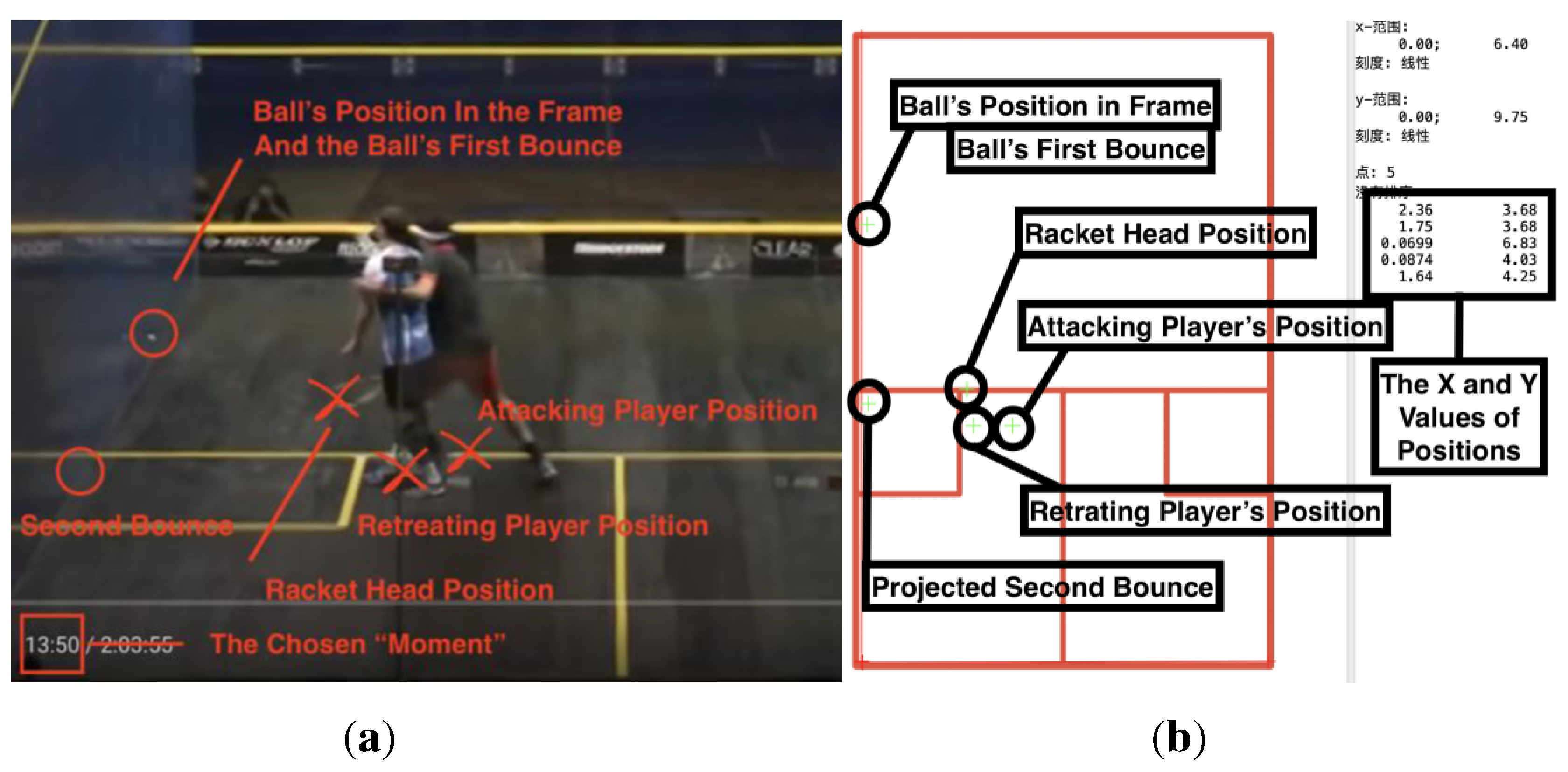
After a moment is selected, six data components are collected from the frame: the attacking player’s position, the retreating player’s position, the ball’s position in the frame, the ball’s projected first bounce, the ball’s projected second bounce, and the attacking player’s racket head position.
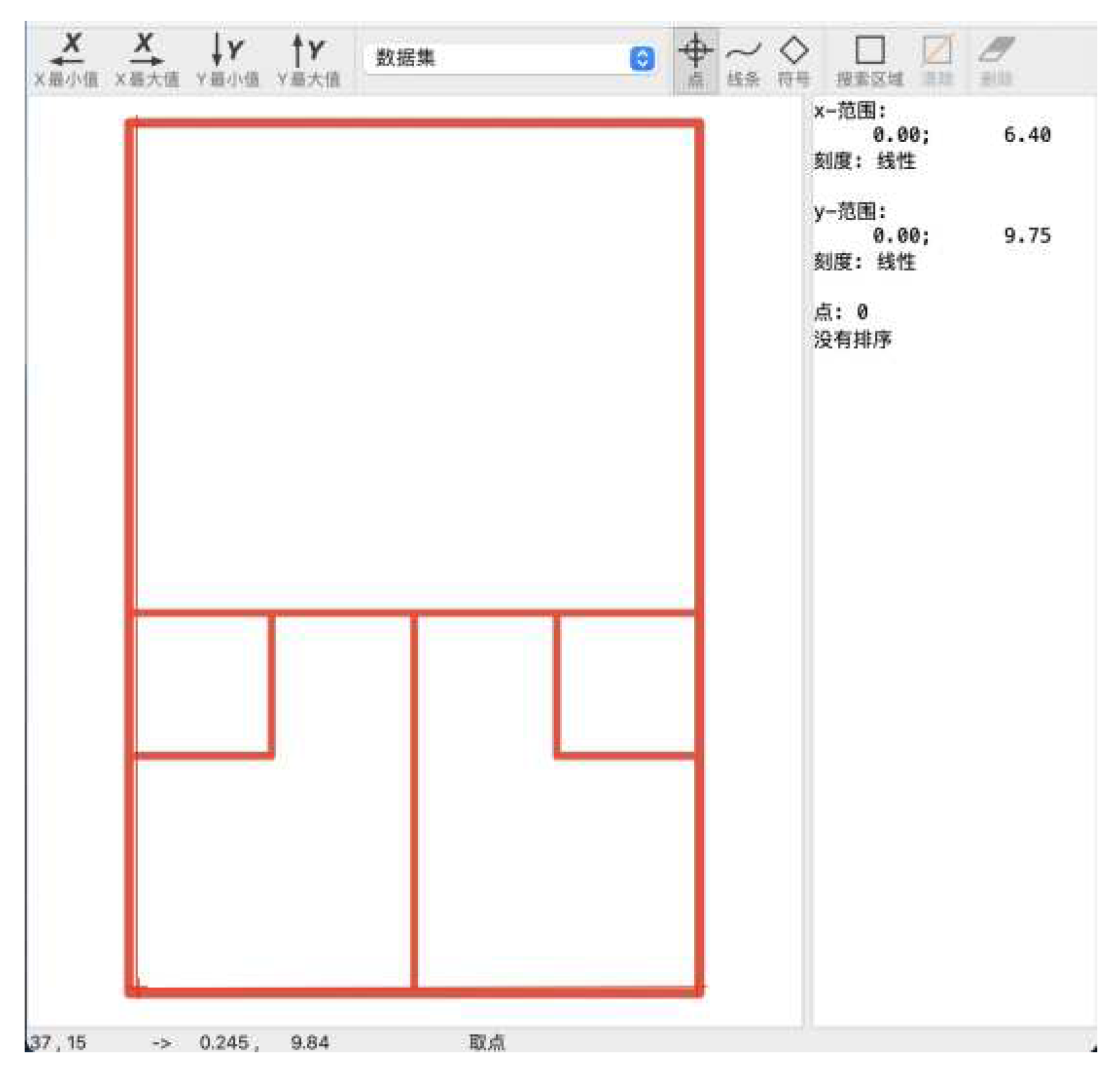
To collect this data, we used the tool Digitizeit. Inside Digitizeit, a top-down view of a standard squash court is uploaded. The x-axis and the y-axis are defined to begin at the bottom left of the squash court. A standard squash court’s dimensions are 6.40 meters in width and 9.75 meters in length. The x-axis ranges from 0 (meters) to 6.40 (meters), and the y-axis ranges from 0 (meters) to 9.75 (meters).
Figure 4.
Screenshot of the tool Digitizeit.
To collect the six data components, we plot a point on the graph of the squash court and Digitizeit labels its X and Y values. These values are then collected into our dataset together with the final decision. For instance:
Figure 5.
(a) Data #3, Gaultier/Elshorbagy 2014 ElGouna 13:50 YesLet [17]. The above format means: The Data Labeled “3” in our dataset. Taken from the match between Gregory Gaultier and Mohamed Elshorbagy in the 2014 ElGouna Championships. The interference happened at 13:50 in the video. The final decision is: Yes Let. (b) Labeling for Data #3 in the tool Digitizeit.
2.2. Data Distribution
Four hundred decisions were collected for this study, ranging from multiple years and from multiple world-class players.
Figure 6.
Distribution of data over time.
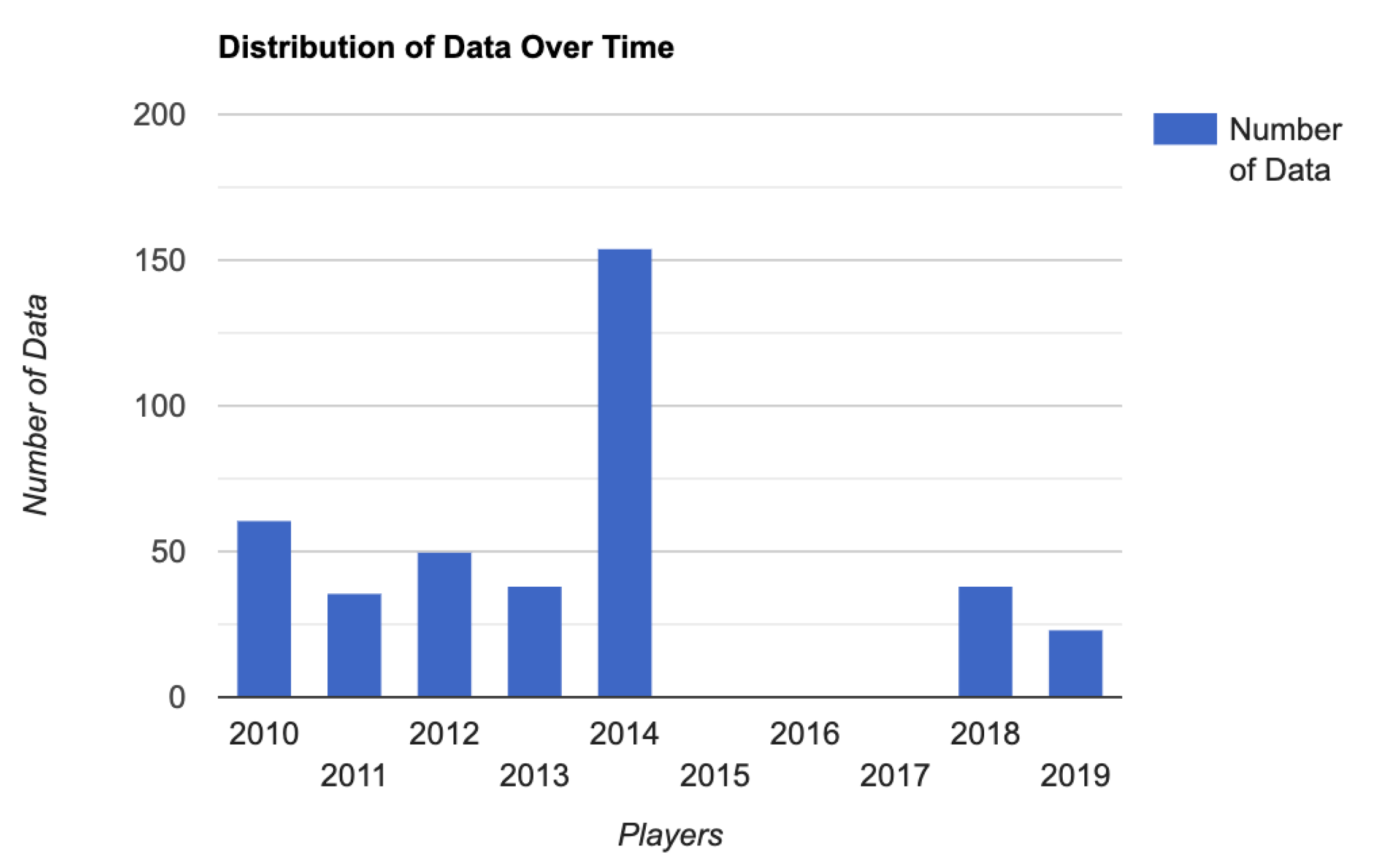
The refereeing standard has shifted over the past decade. By awarding more strokes and punishing more No Lets, the PSA intends to encourage fewer stoppages due to minimal interferences and more continuous plays. Such an effect is visible when reviewing matches from 2018 and 2019. Most of the data in this study are taken from 2010 to 2014, approximately when the video review system was available and when the refereeing standard was approximately consistent [18].
Figure 7.
Distribution of data over players.
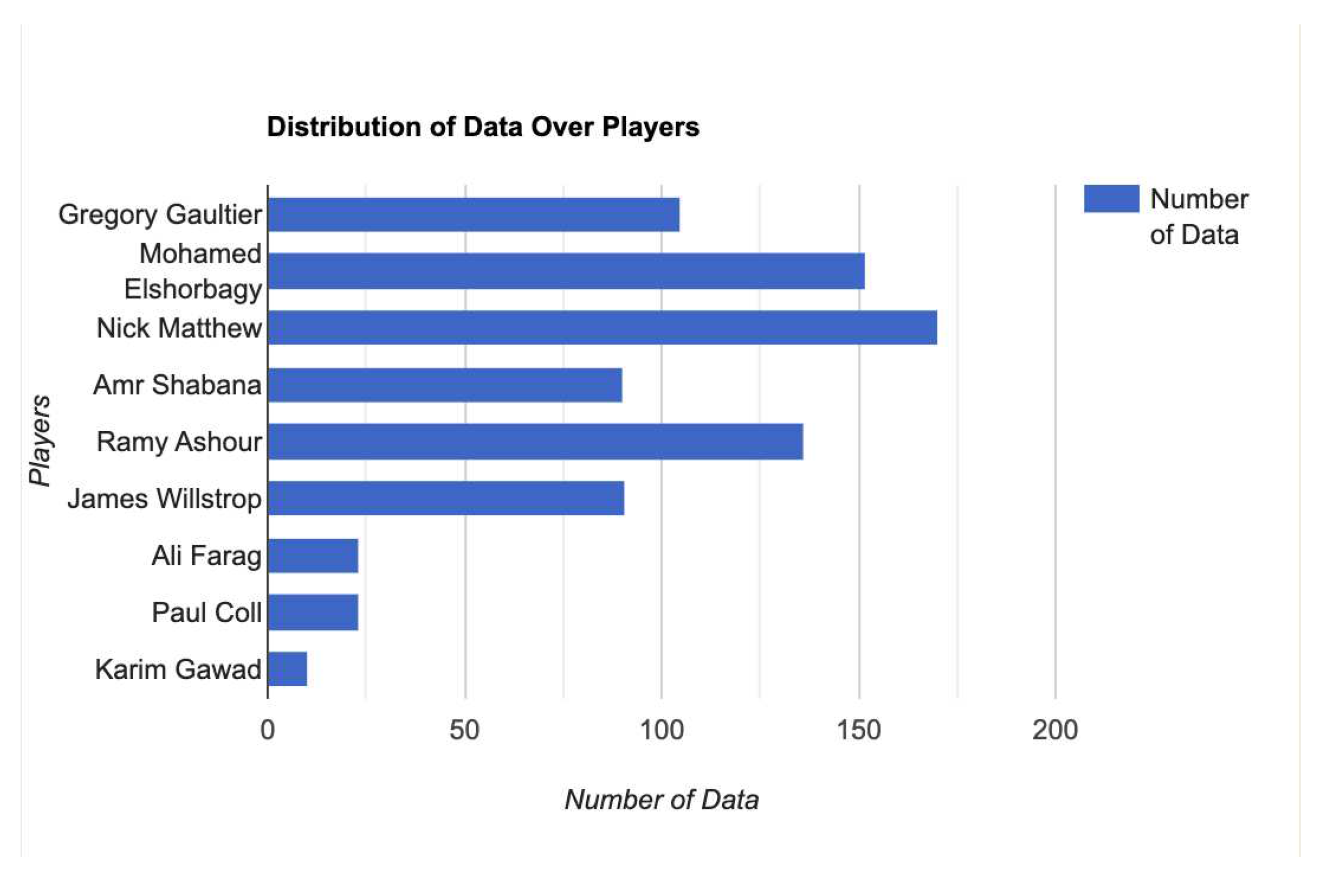
Due to factors such as the style of play, body strength, shot selection, dominance in the center of the court, and movement style, some players might be involved in more interference than others. We tried to collect approximately similar numbers of decisions from each player involved.
The involved players are all among the best in the world. All have reached world number one at some point in their career and are all winners of major titles for squash.
Figure 8.
Number of each decision.
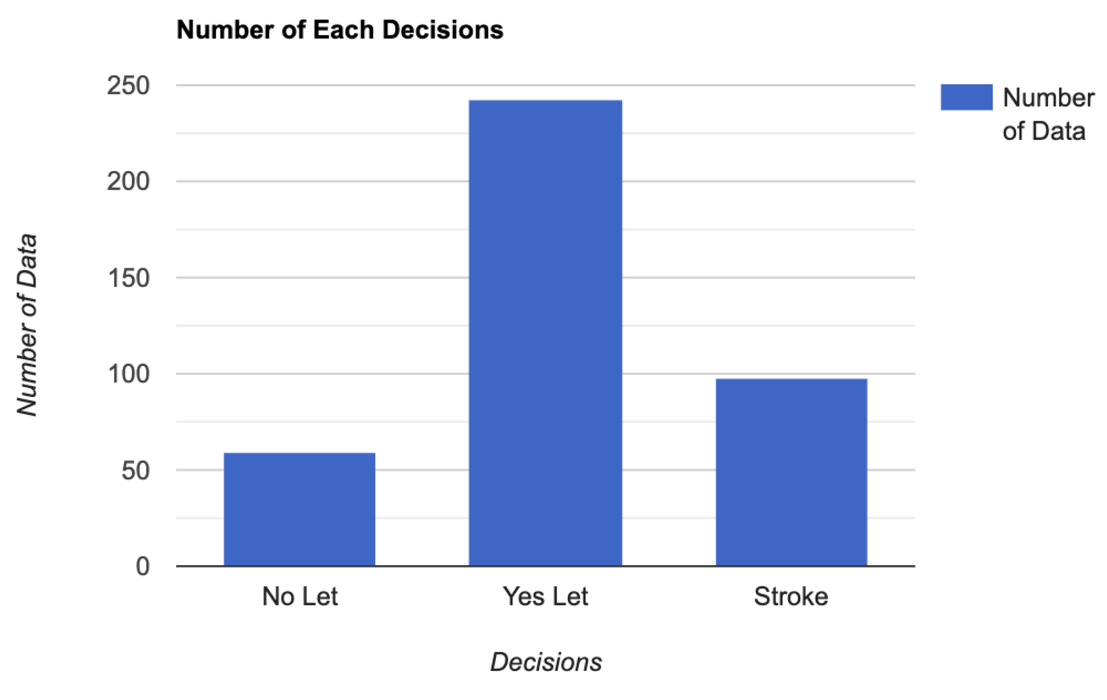
Due to the nature of the game, in any given match, there are more decisions ending in Yes Let than decisions ending in Stroke and No Let. Due to time constraints, we collected as many decisions as we could instead of discarding Yes Lets in search of No Lets and Strokes. As a result, our dataset consists of 59 No Lets, 243 Yes Lets, and 98 Strokes.
3. Methods
3.1. Python, TensorFlow, and Wolfram Mathematica
This study will use two programming platforms to train the model: Python and Wolfram Mathematica. The rationale for selecting Python is that it grants the ability to make many modifications to our model, including the Network layers, nodes, different methods and functions, etc. The TensorFlow package constructs model layers with ease and provides freedom in modifying and fine-tuning the model. The combination of Python and TensorFlow has been widely used to train machine learning models. A study in 2019 used TensorFlow and achieved competitive performance results in classifying breast cancer malignancy [19]. A study in 2021 used TensorFlow and compared artificial neural networks and convolutional neural networks in image classification tasks [20].
Wolfram Mathematica, on the other hand, is easy to program and provides useful visualizations for model performances. Previous studies have successfully used this tool to train powerful models. A study in 2022 used Wolfram Mathematica’s system and developed an algorithm for localizing car license plates [21]. A study in 2021 used Wolfram Mathematica and produced Covid-19 projections by using a machine-learning method with cumulative data for confirmed infected patients, deaths, and vaccinated patients in Mexico during 2021 [22].
The results of this study are, therefore, separated into the Python sections and the Wolfram Mathematica sections.
3.2. Neural Network
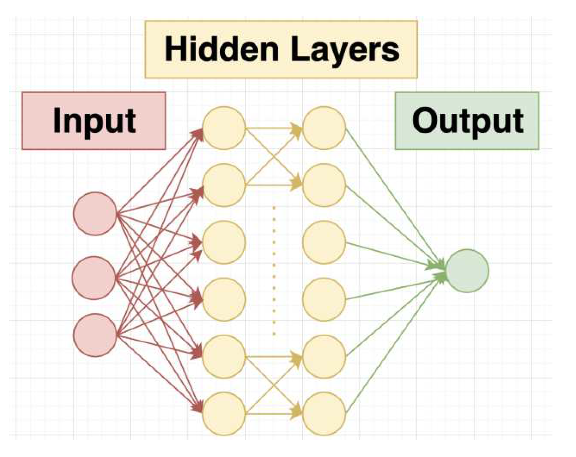
This study implements machine learning through neural networks. Neural networks are machine learning algorithms inspired by the human brain and simulate the connection between neuron cells. Through layers of fully connected nodes, with each node performing a simple calculation task of multiplication and addition of parameters, the inputs go through numerous calculations and reach a final value or the intended answer. After being trained using a large amount of data, a neural network can perform classification or clustering tasks in a very short period of time.
Figure 9.
Illustration of a neural network’s structure.
3.3. Normalization
To pre-process the dataset, this study explores the technique of normalization. Normalization is a technique often used in machine learning to set a common scale for data with different ranges and measures. For this study specifically, although all X-values share a common measure (0m to 6.4m) and all Y-values share a common measure (0m to 9.75m), it is worth exploring whether the two axes could be normalized to allow the model to perform better.
3.4. Selection from the Six Data Components
As there exist many complicated reasons as to why a situation results in a decision, a neural network may be unable to learn all the relations between all data component values. Dropping out some less meaningful data components may, in fact, help the model to perform better, as some too much information could act as a noise to the model and impede its improvement.
3.5. Modified Data Points
We hypothesized that the initial six data components (or, the primitive data components) would not be enough to achieve the accuracy needed in real-life squash refereeing. There are more than six factors that decide what should be the right decision for an interference. Therefore, we decided to calculate a second layer of data using the primitive components we had acquired. The second layer of data components may be able to provide more insights into why and how a situation is considered one of the three decisions. More specifically, we used the primitive data components and calculated nine more values which we think can provide useful information. The second layer of data components is explained below:
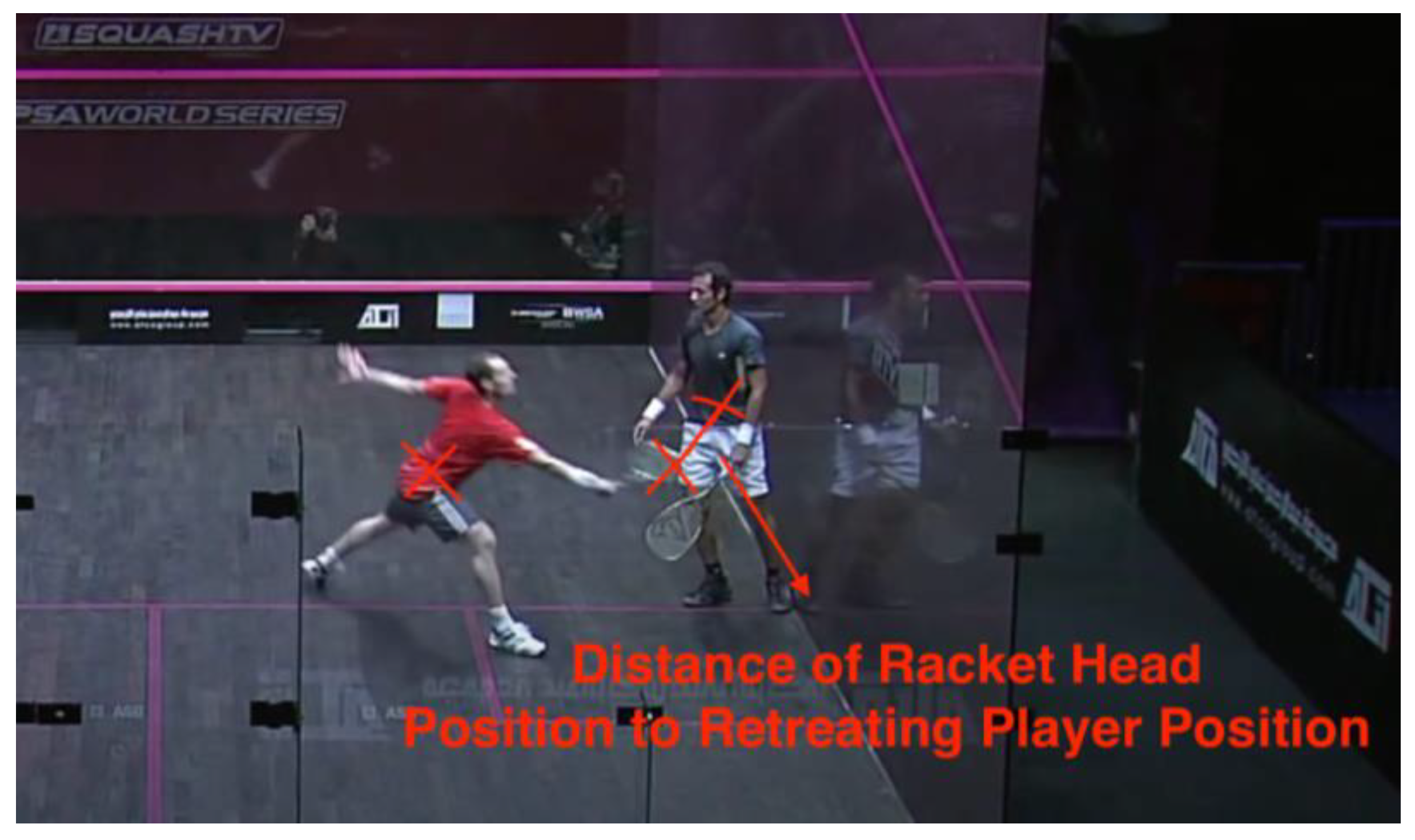
3.5.1. Distance of Attacking Player (AP) to Retreating Player (RP)
The distance between two players is calculated through the Pythagorean theorem. This value is included because how close the players are may affect how the decision is made, especially in situations where no physical contact is presented but the ability to play the ball is impeded. This value may provide less useful information in cases where physical contact occurs, as in those situations the distance tends to be short as the players’ bodies have made contact.
Figure 10.
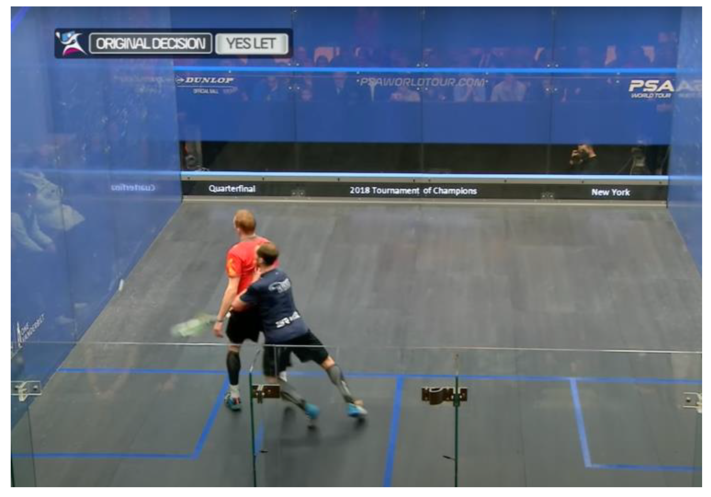
(a) Data #402, Gawad/Willstrop 2018 Grasshopper 1:02:48 Stroke [23]. (b) Data #92, Matthew/Shabana 2014 Tournament of Champions (ToC) 1:35:10 Yes Let [24].
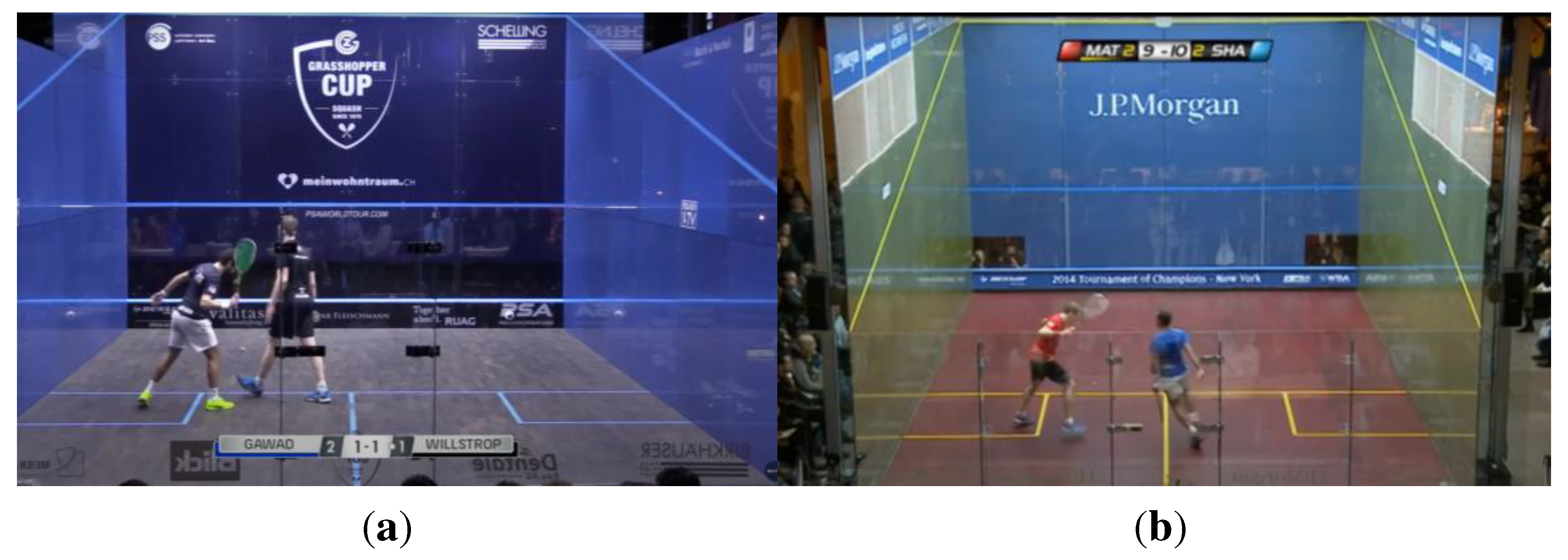
The above two cases are a great demonstration of how distance between players can cause the decision to change. In both scenarios, the player location and the ball locations are similar, yet the former is decided a Stroke and the latter a Yes Let. This is because in the first scenario, the two players are very closely positioned. If the attacking player was going to play the ball, he would likely strike his opponent. Therefore, a stroke is awarded to the attacking player. In the second scenario, there is more space between the two players, and the attacking player would have space to hit the ball without hitting his opponent. Therefore, the referees deemed the situation as Yes Let.
3.5.2. Distance of Attacking Player to Ball Position in Frame
The distance of AP to the ball provides useful information in making decisions. If the ball is close to the AP, there is more possibility of the decision being a stroke; the further the ball is from the AP, the higher the chance of the decision being a No Let. The distance can be a good indicator of the attacking player’s ability to play the ball. There are fewer chances of No Lets if the attacking player is ready to play the ball instead of being on the way to the ball.
However, the ball position may not be a good indicator of where the player will play the ball. In situations where the ball travels to the back of the court and the interference happens when the ball is in the middle, the distance of AP to the ball can provide information about where the player will be playing the ball. In situations where the ball stays up in the court, the distance of AP to the ball can be misleading because the ball position in frame will travel towards the player and end at the second bounce position. In this case, where the player will play the ball is closer to the player than the ball position in frame, and the distance of AP to the ball is exaggerated.
Figure 11.
Data #4, Gaultier/Elshorbagy 2014 ElGouna 19:57 YesLet [17].
Figure 11.
Data #4, Gaultier/Elshorbagy 2014 ElGouna 19:57 YesLet [17].
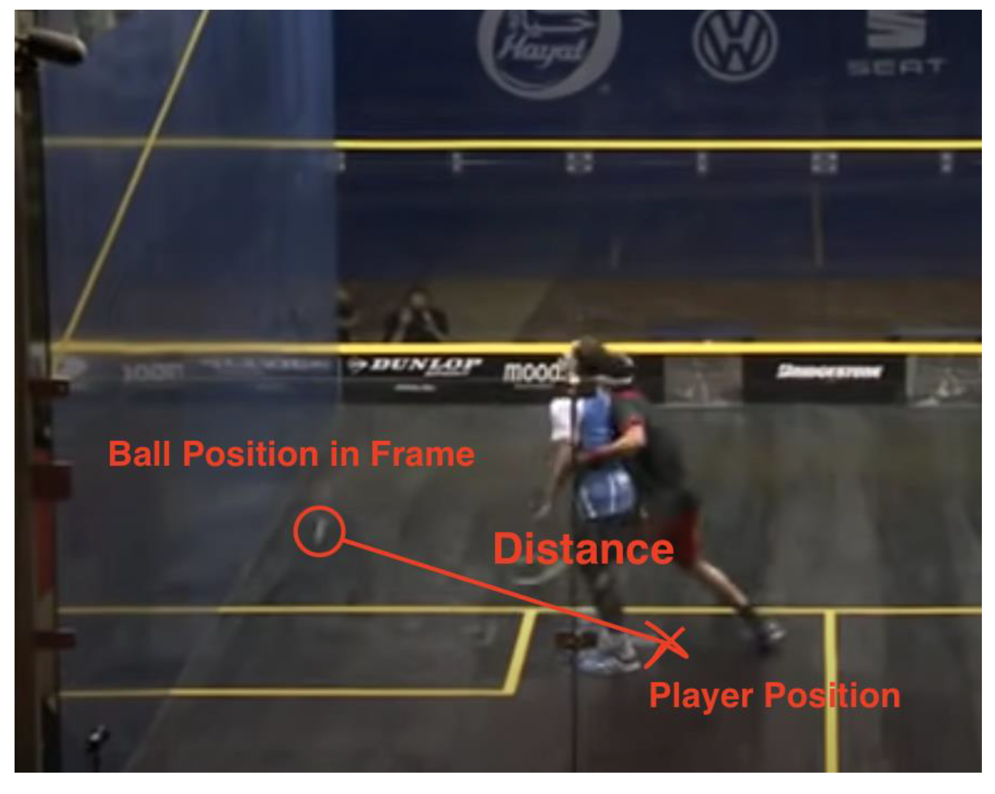
The above situation is a case in which this information can be a useful tool, as the ball position in frame is close to where the player is going to play it. The distance therefore provides insights into the player’s ability to get to the ball.
Figure 12.
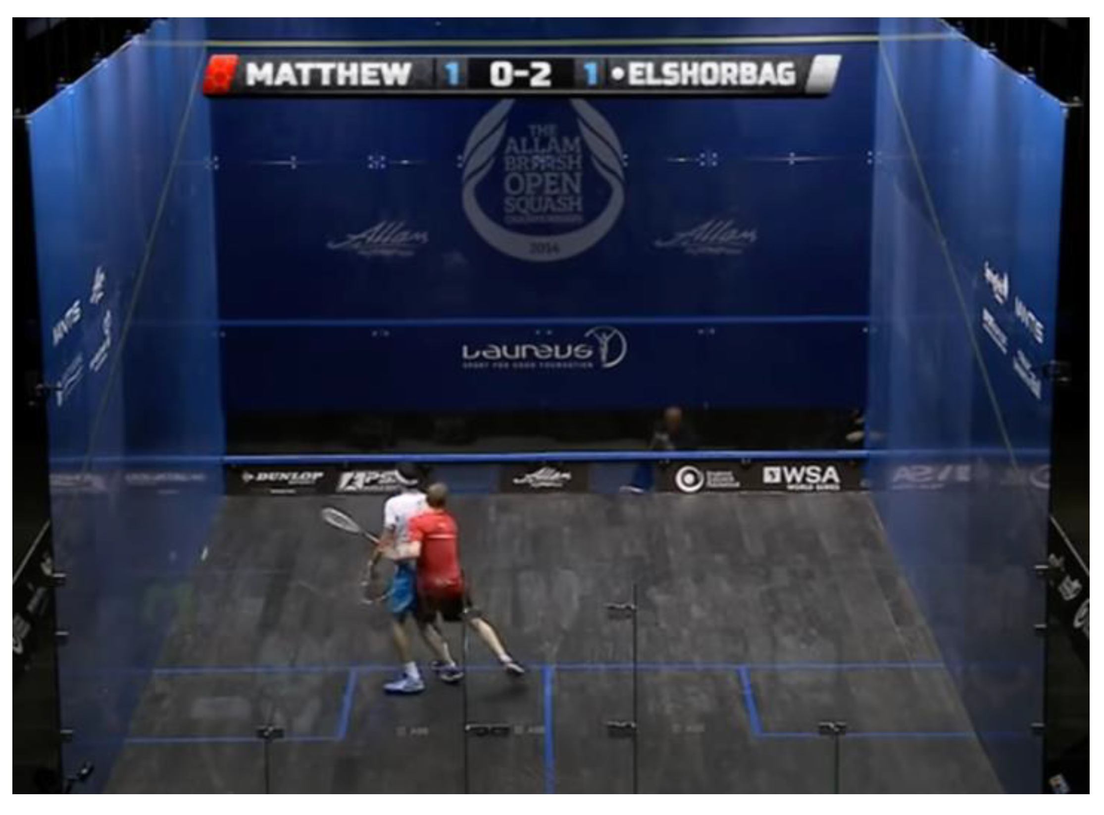
Data #39, Matthew/Elshorbagy 2014 British Open 49:11 Yes Let [25].
Figure 12.
Data #39, Matthew/Elshorbagy 2014 British Open 49:11 Yes Let [25].
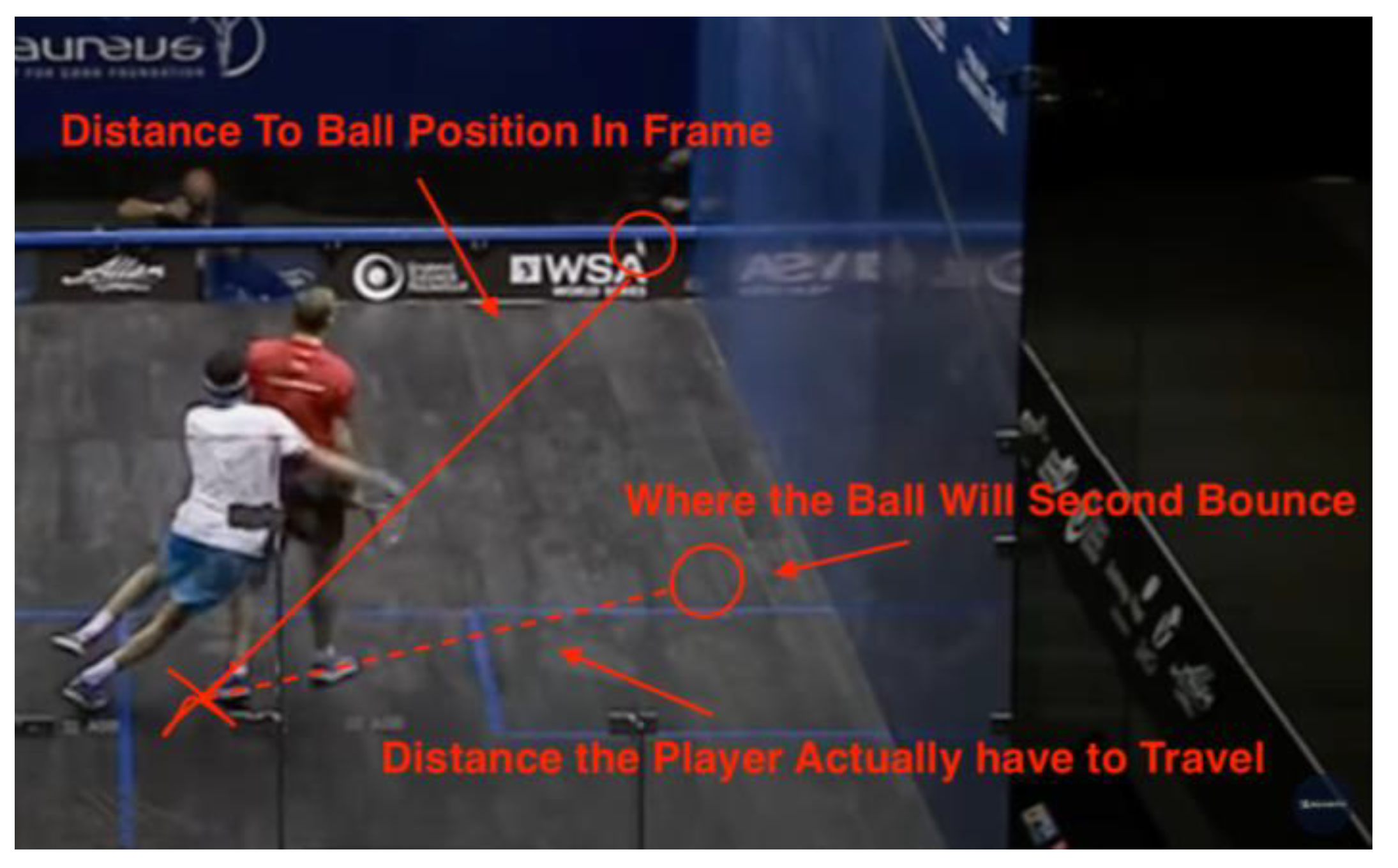
This situation is a case in which the information can be misleading. The ball travels towards the attacking player, therefore, the ball position in frame is a lot further than the distance the attacking player actually has to travel.
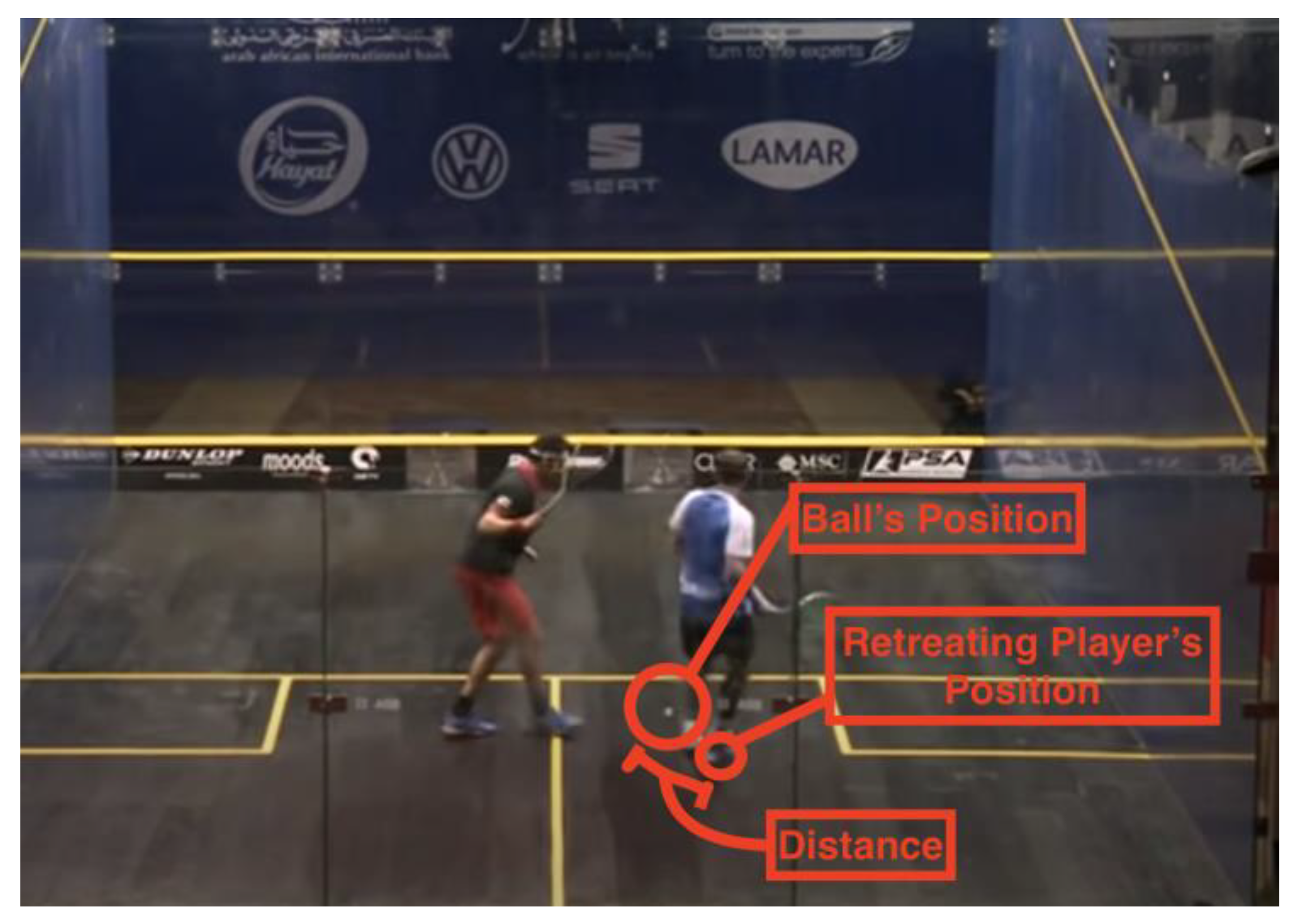
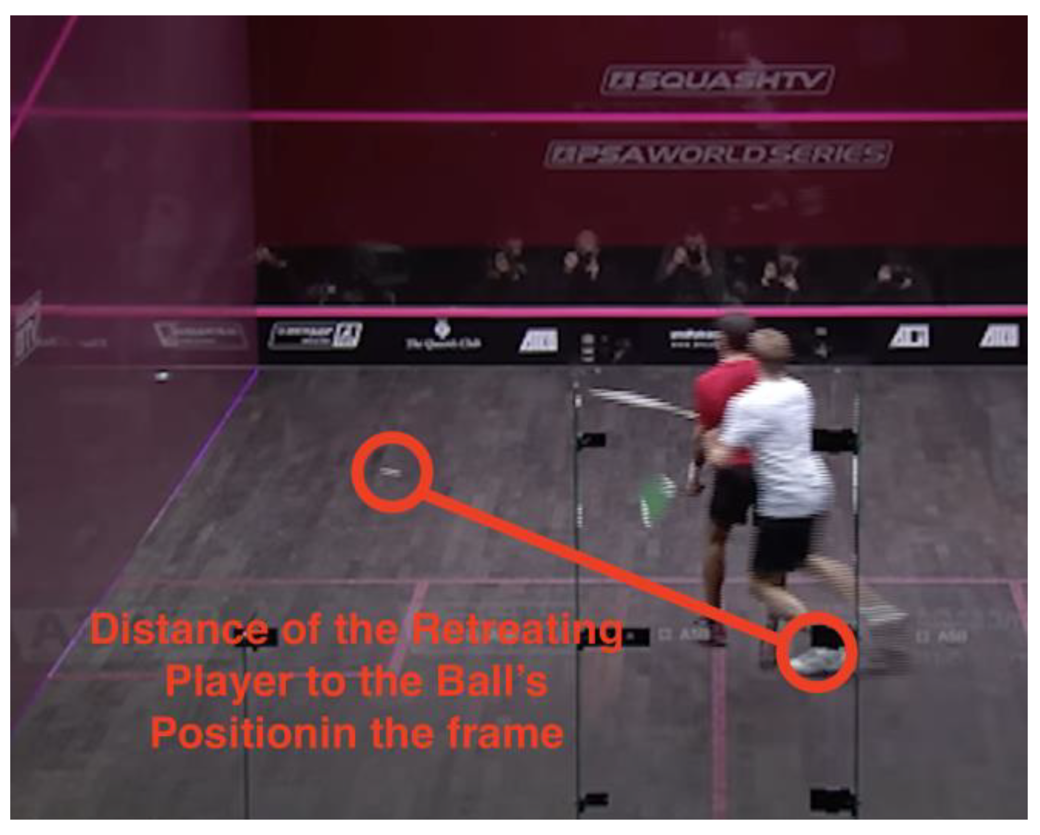
3.5.3. Distance of Retreating Player to Ball Position in Frame
The distance of the retreating player to the ball can provide information about how much the RP is blocking access to the ball. If the RP is away from the ball, the situation should lean away from a stroke. If the RP is right next to the ball, it shows that the RP is blocking access to the ball, which would push the decision towards a stroke.
Similar to the distance of AP to ball position in frame, this value may not be a good indicator of where the attacking player can play the ball. If the ball position in frame is next to the RP, but the AP is still too far away to play the ball, the situation can be considered a Yes Let or No Let. On the other hand, if the ball position in frame is away from the RP, but it will eventually end next to the RP, the situation can still be considered a Stroke.
Figure 13.
Data #25, Gaultier/Elshorbagy 2014 ElGouna 1:42:50 Stroke [17].
Figure 13.
Data #25, Gaultier/Elshorbagy 2014 ElGouna 1:42:50 Stroke [17].
This example shows how the distance of RP to the ball can be a good indicator that the situation is a stroke. In this case, the RP accidentally hits the ball back to himself, and the AP would have hit him had he attempted to swing at the ball. Therefore, because the distance of RP to the ball is small, this situation is considered a stroke.
Figure 14.
Data #364, Shabana/Matthew 2013 World Tour Finals 1:00:33 No Let [26].
Figure 14.
Data #364, Shabana/Matthew 2013 World Tour Finals 1:00:33 No Let [26].
This situation shows that the distance of RP to the ball can also be an indicator if the situation is a No Let. In this case, the RP is very far away from the ball, which suggests that the AP created his own interference by going directly at the RP, or the AP could not have reached the ball had there been no interference. In either case, the decision would be No Let.
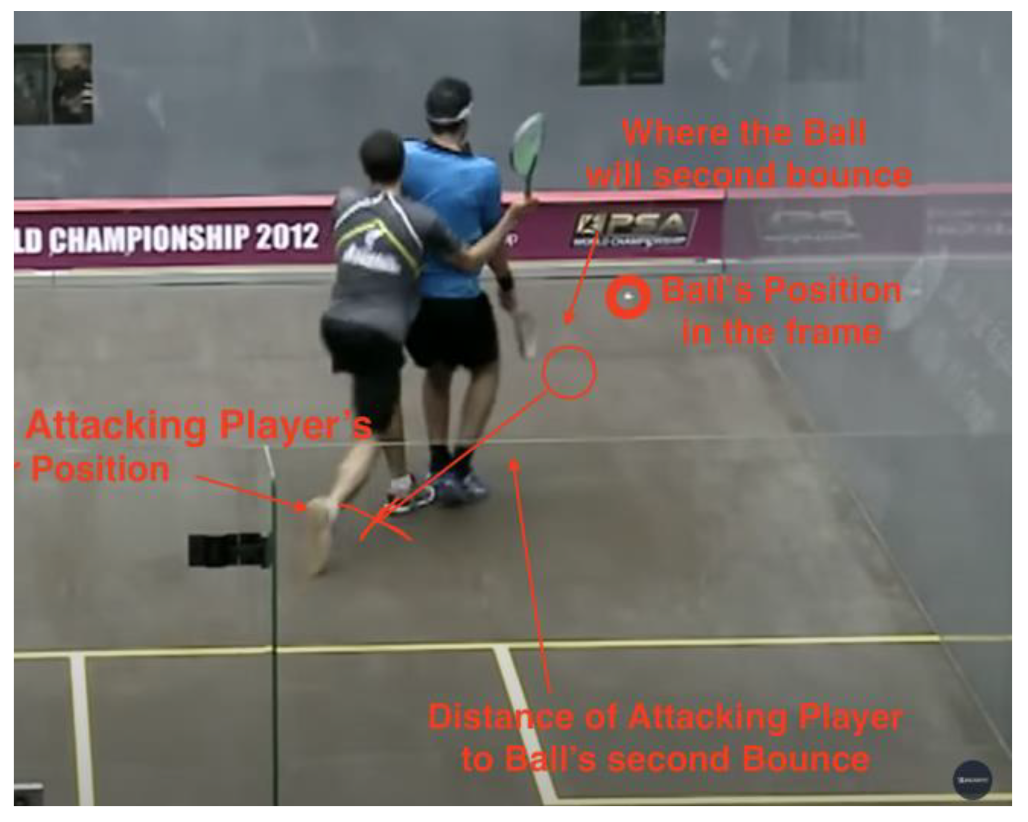
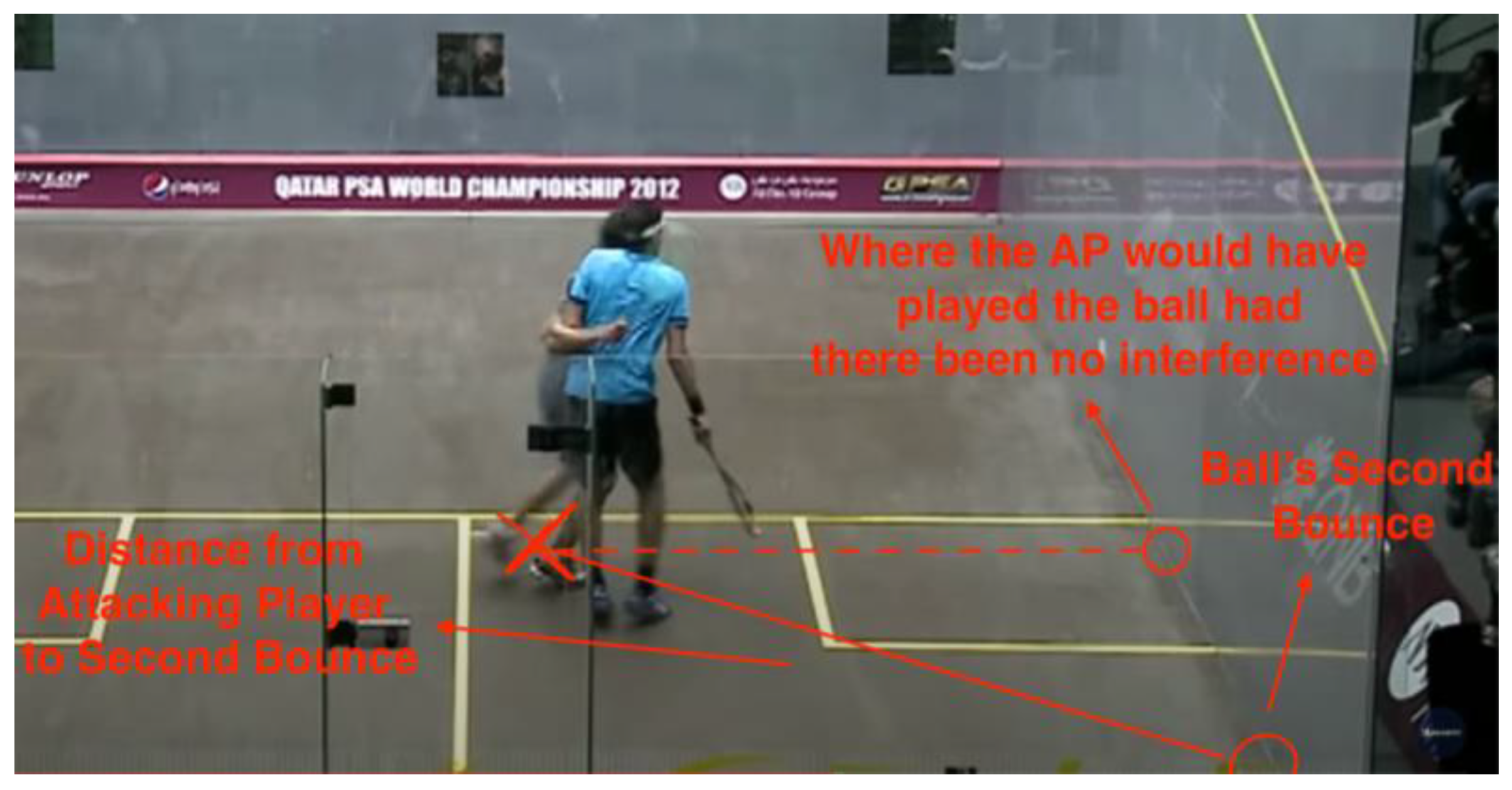
3.5.4. Distance of Attacking Player to Second Bounce
Usually, the referee looks at the second bounce to determine how far away the ball is from the players. By considering the distance of the AP to the second bounce, we can gain information about how much the attacking player has to move before arriving at a position to play the ball. This value can be very straightforward when the ball remains at the front of the court: the closer it gets to the AP, the higher the chance it is a stroke.
However, when the ball travels to the back of the court, at some point the ball is closest to the attacking player, and it will travel away. Had there been no interference, the attacking player would ideally play the ball where it is closest to him instead of following the ball until its second bounce. In this case, the distance of AP to the second bounce position again fails to identify the position where the player is going to play the ball.
Figure 15.
Data #142, Ashour/Elshorbagy 2012 World Championship 1:30:41 Stroke [27].
Figure 15.
Data #142, Ashour/Elshorbagy 2012 World Championship 1:30:41 Stroke [27].
In the case above, the distance of the attacking player to the second bounce supports why the decision is a Stroke. Where the ball lands for its second bounce is really close to the AP, which means the AP could easily play the shot, had there been no interference. Since the retreating player is directly in the way, this is one of the most obvious stroke decisions.
Figure 16.
Data #134, Ashour/Elshorbagy 2012 World Championship 1:13:29 Yes Let [27].
Figure 16.
Data #134, Ashour/Elshorbagy 2012 World Championship 1:13:29 Yes Let [27].
This is a case where the distance of the attacking player to the second bounce is an inaccurate representation of the attacking player’s ability to get to the ball. Had there been no interference, the AP would have played the ball around the service box. If we consider the distance to the second bounce, the AP would be unjustly evaluated for his ability to retrieve the ball, since he only has to move to the service box instead of having to move to the back of the court.
3.5.5. Distance of Racket Head to Retreating Player
If the swing of a player is impeded by the other player and he would have been able to play the ball otherwise, a Stroke would be awarded to the player. The distance of the racket head to the retreating player aims to capture this aspect of decision-making. If the racket head is close to the retreating player and the ball is close to the AP, the situation will likely be a Stroke.
Figure 17.
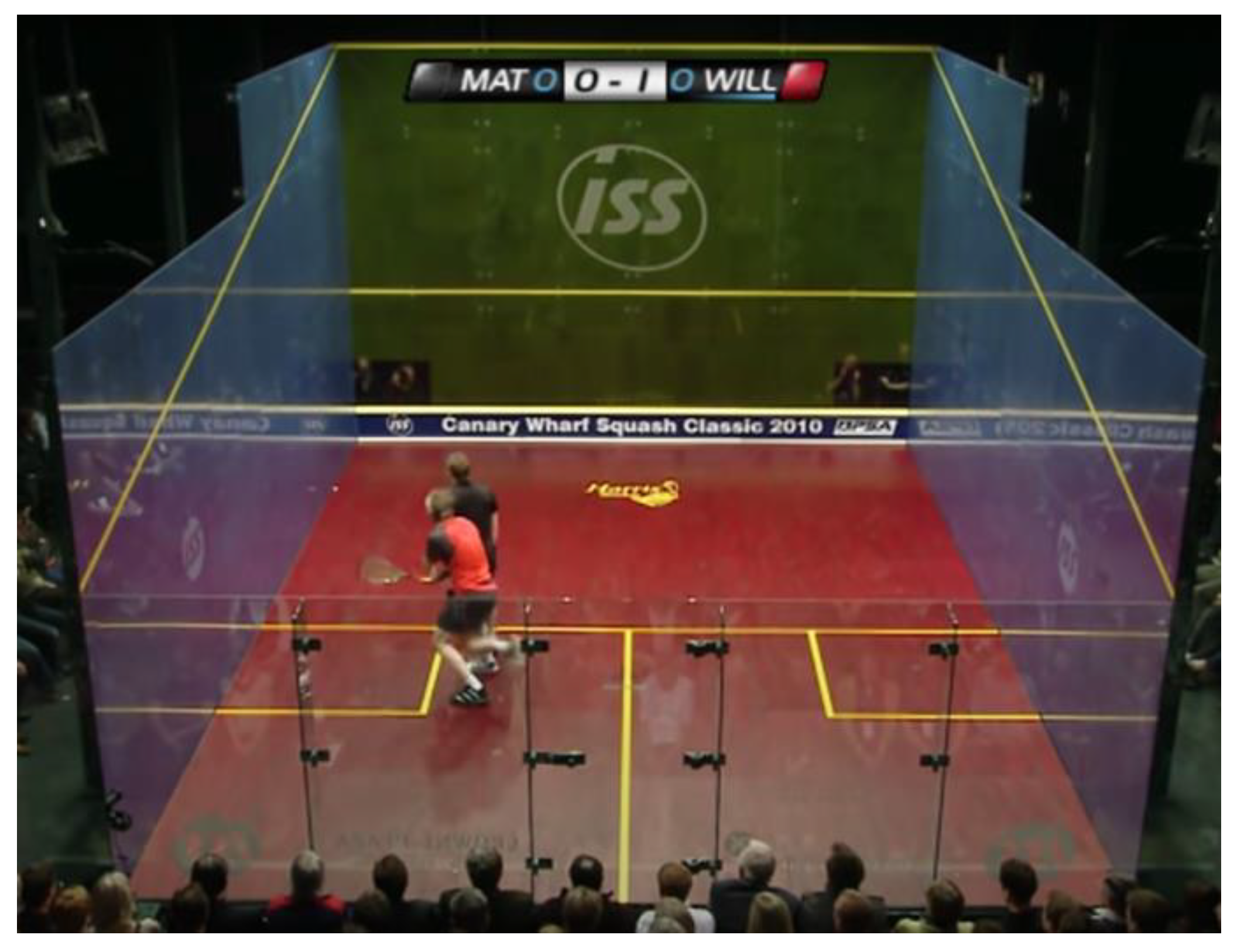
Data #192, Matthew/Willstrop 2010 Canary Wharf 1:41:18 Stroke [28].
Figure 17.
Data #192, Matthew/Willstrop 2010 Canary Wharf 1:41:18 Stroke [28].
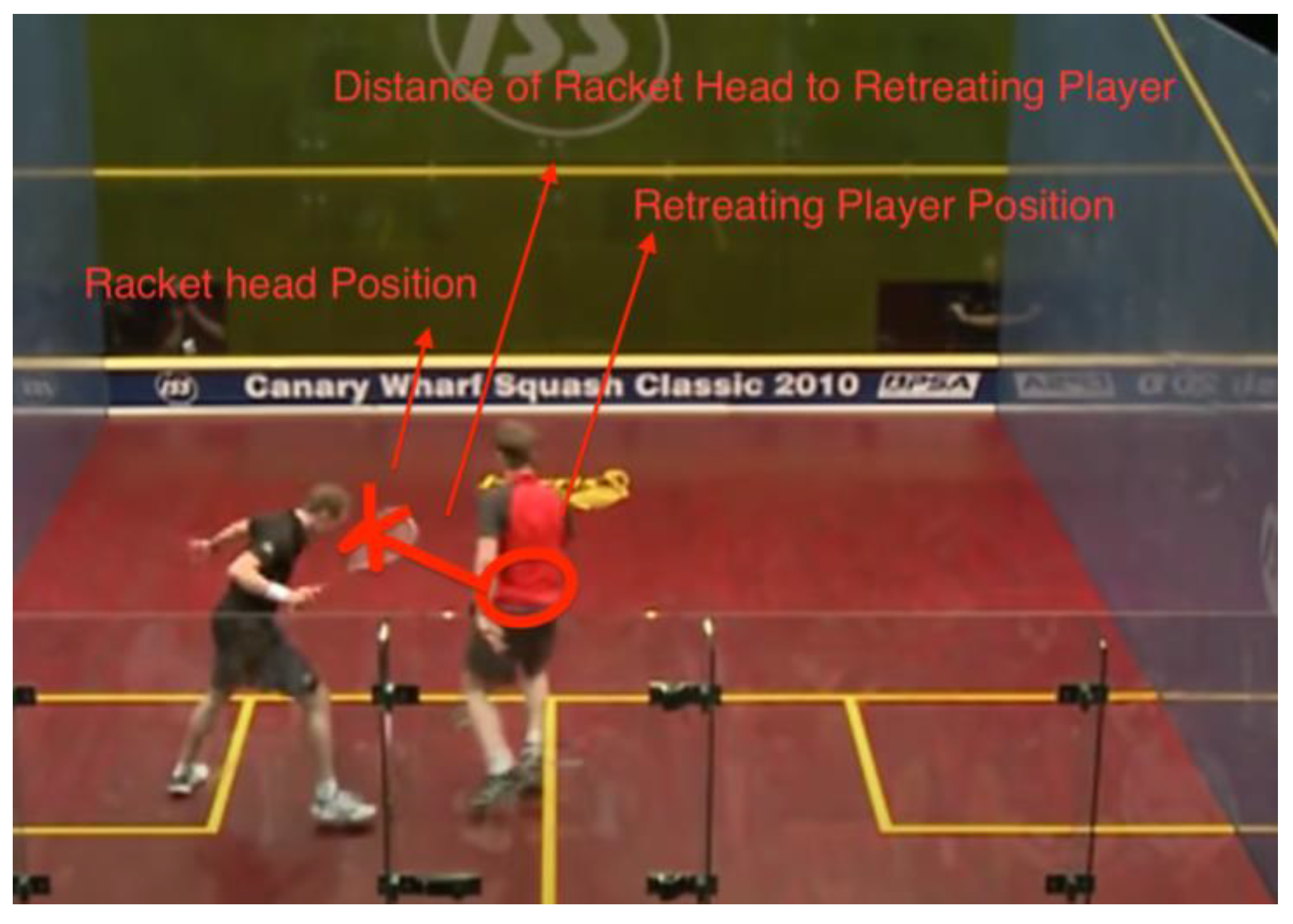
This is an example of the racket head being too close to the retreating player, and the referee deemed the situation a stroke. Had the AP swung at the ball, the RP would likely have been hit. After all, this distance provides similar information to the Distance of AP to RP, but we hypothesize that this may provide a more accurate value.
3.5.6. Distance of the Ball Position in Frame to Second Bounce
In making decisions, the referee considers the “quality of shot.” If there is interference, yet the shot is “too good,” the referee makes the decision of No Let. This value aims to present information about how good the ball is. The distance of the ball position in frame to the second bounce shows how far the ball travels before it dies, and therefore indirectly provides information about how much time the player has to retrieve the ball if there has been no interference, or the “time remaining.” If the contact happened and the ball died right away, the AP could not have gotten to the ball, even if there was not any interference. On the other hand, if there is still lots of time until the ball dies after the interference, the situation is likely a Yes Let.
Figure 18.
Data #167 Matthew/Willstrop 2010 Canary Wharf 1:02:50 No Let [28].
Figure 18.
Data #167 Matthew/Willstrop 2010 Canary Wharf 1:02:50 No Let [28].
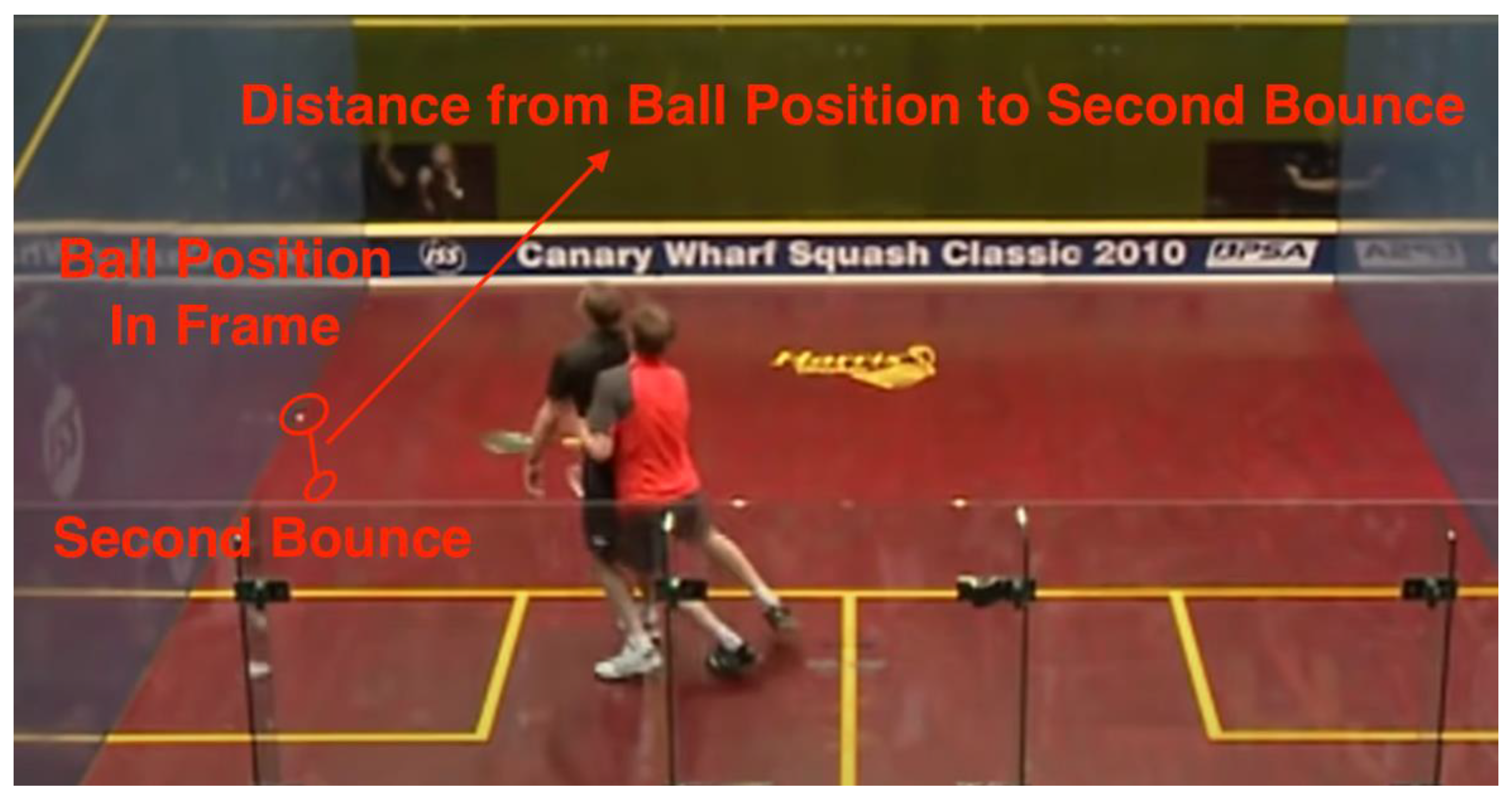
This situation demonstrates how this information can be used to determine No Let. As the ball hits the “nick” on the first bounce (the “nick” is the corner between the floor and the wall. When a ball lands in the nick, energy is taken away and it can die very quickly), the ball stays very short, which leaves no time for the AP to retrieve the shot. Because the distance of ball position to second bounce is short, the referee deemed the situation a No Let, as the AP could not reach the ball even if there was not any interference.
3.5.7. Distance of Racket Head to Ball Position in Frame
This value provides similar information to the distance of the attacking player to the ball position in frame. We included this information because sometimes the reach of the player can be long enough to reach the ball even when their body is more than a meter away. The racket head position may provide more useful information about the attacking player’s ability to play the ball than the attacking player’s position.
Figure 19.
Data #214, Shabana/Gaultier 2011 World Series Finals 33:09 Stroke [29].
Figure 19.
Data #214, Shabana/Gaultier 2011 World Series Finals 33:09 Stroke [29].
This case is an example of why the distance of racket head to ball position may provide a better notion of the attacking player’s ability to play the ball than the distance of attacking player to ball position. In this case, the AP’s racket head is very far away from his body. He is fully stretched and can strike a ball that is more than one and a half meters away from him. In this case, simply calculating the distance of the AP to the ball may provide a false sense that the AP is still some distance away from the ball, Therefore, we decided to include this value.
3.5.8. The Shortest Distance from Racquet Head to The Path of Ball
For multiple values described above, the limitation of “not able to identify where the AP is going to play the ball” exists. This value aims to resolve the issue by calculating the shortest distance from the path of the ball to the AP’s racket head. The path of the ball is defined as the straight line segment from the ball position in frame to the second bounce position. We define the shortest path to be the line which originated from the racket head position and is perpendicular to the ball’s path. If the line intersects the ball path (as the ball path is a line segment and could end before the intersection happens), we calculate the distance from the racket head position to the intersection. If the intersection does not exist on the line segment, we take the closest ending point (either second bounce or ball position) on the line segment and calculate the distance from it to the racket head position.
Figure 20.
Data #283 Gaultier/Ashour 2013 British Open 22:55 Yes Let [30].
Figure 20.
Data #283 Gaultier/Ashour 2013 British Open 22:55 Yes Let [30].
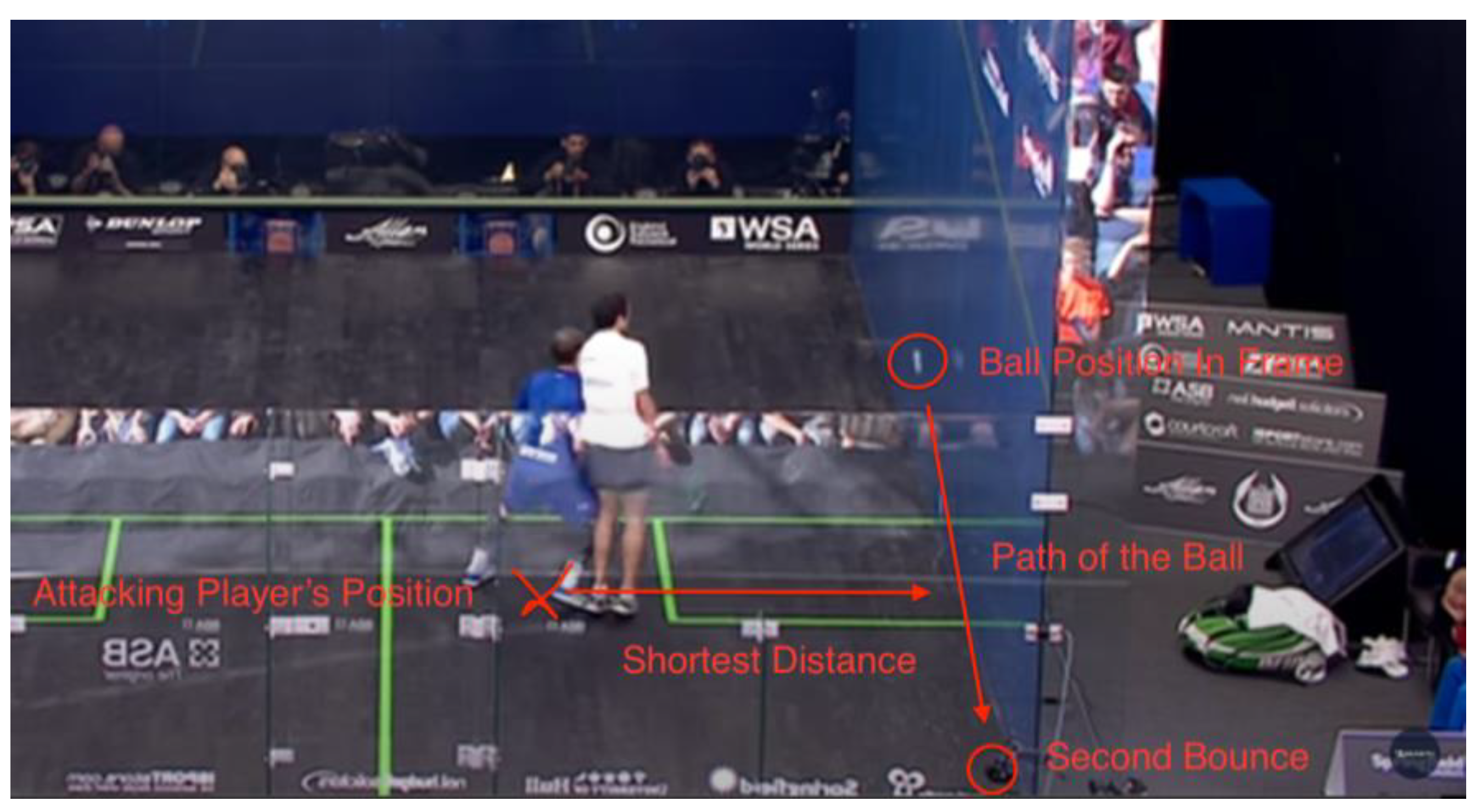
This is an example of the shortest distance to the ball’s path. If there was not any interference, the AP would have chosen to approach the ball through the path with the shortest distance (which is the line perpendicular to the path) instead of going all the way to where the ball bounces.
Figure 21.
Data #390 Farag/Coll 2019 British Open 1:05:40 Yes Let [31].
Figure 21.
Data #390 Farag/Coll 2019 British Open 1:05:40 Yes Let [31].
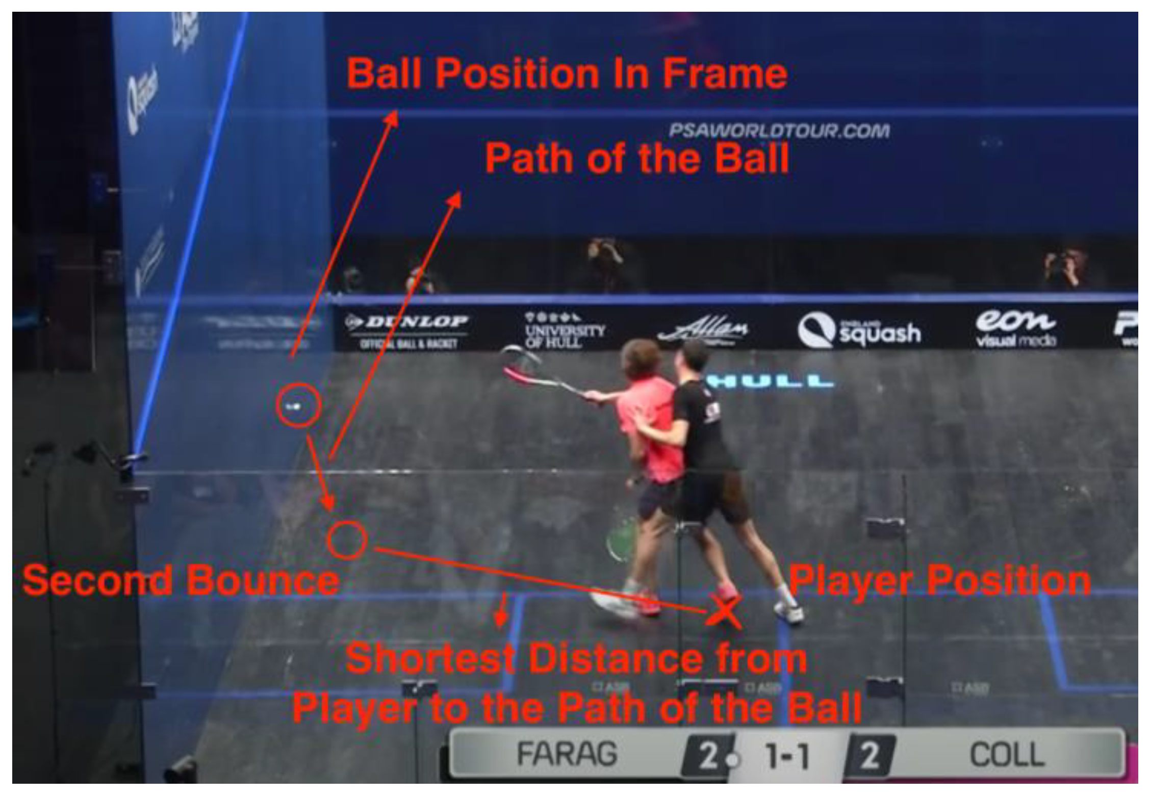
In this case, the shortest distance to the path of the ball is the distance to the second bounce position. Because the perpendicular line to the ball’s path originating from the AP’s position does not intersect with the line segment (does not exist on the path), we take the closest ending point of the segment (either ball position in frame or second bounce position) as the closest point.
3.5.9. Access to the Front Wall: How Much is Blocked by the Other Player
When the RP blocks the AP’s access to the front wall, the situation is considered a Stroke. This rule is sometimes compromised when the blockage is little or the AP is not able to make shots due to the speed or the position of the ball. Although it is not a clear-cut situation, a significant blockage of the front wall is still considered a Stroke. We calculated the blockage by drawing lines from the AP to both sides of RP, offset by the player’s body width, and analyzing where the lines meet the front wall. For this study, we defined the body width as 80 cm, as the average shoulder width for men is around 40 cm, and we added 40 cm of width to the total width due to the arms and the legs on each side [32].
Figure 22.
Data #118, Elshorbagy/Ashour 2012 World Championship 23:16 Stroke [27].
Figure 22.
Data #118, Elshorbagy/Ashour 2012 World Championship 23:16 Stroke [27].
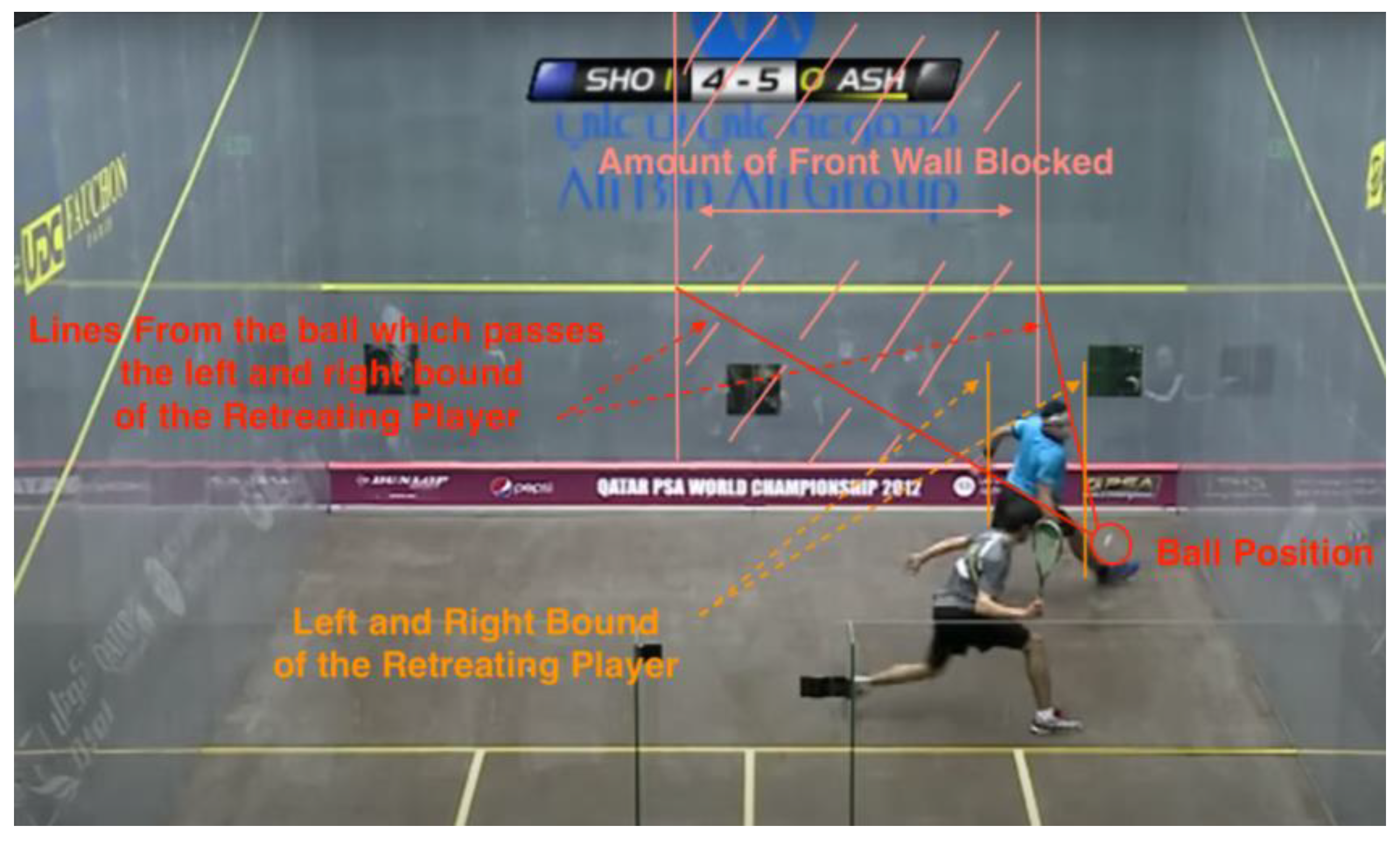
This is an example of how the amount of blockage on the front wall is calculated. Two imaginary lines are drawn from the ball passing the bounds of the RP and reaching the front wall. The final blockage is the width of the area (labeled in pink) inside the two lines.
4. Results
4.1. Results with Mathematica
4.1.1. Experimental Design
Out of the 400 decisions, 60 decisions are taken out as the test set and 340 remain as the training set. The dataset is shuffled before the test set is taken out. As the dataset is small in number and each shuffle may cause big percentile changes to the testing set, every experiment will be done five times to have a better understanding of the average model performance.
We used the built-in functions provided by Mathematica, which is the classify function through application of neural networks [33].
4.1.2. Model Performance on Primitive Data Components
4.1.2.1 Training on All Six Data Components
Figure 23.
A trial of the five models trained on all six data components (for remaining four trials, see Appendix A).
Figure 23.
A trial of the five models trained on all six data components (for remaining four trials, see Appendix A).
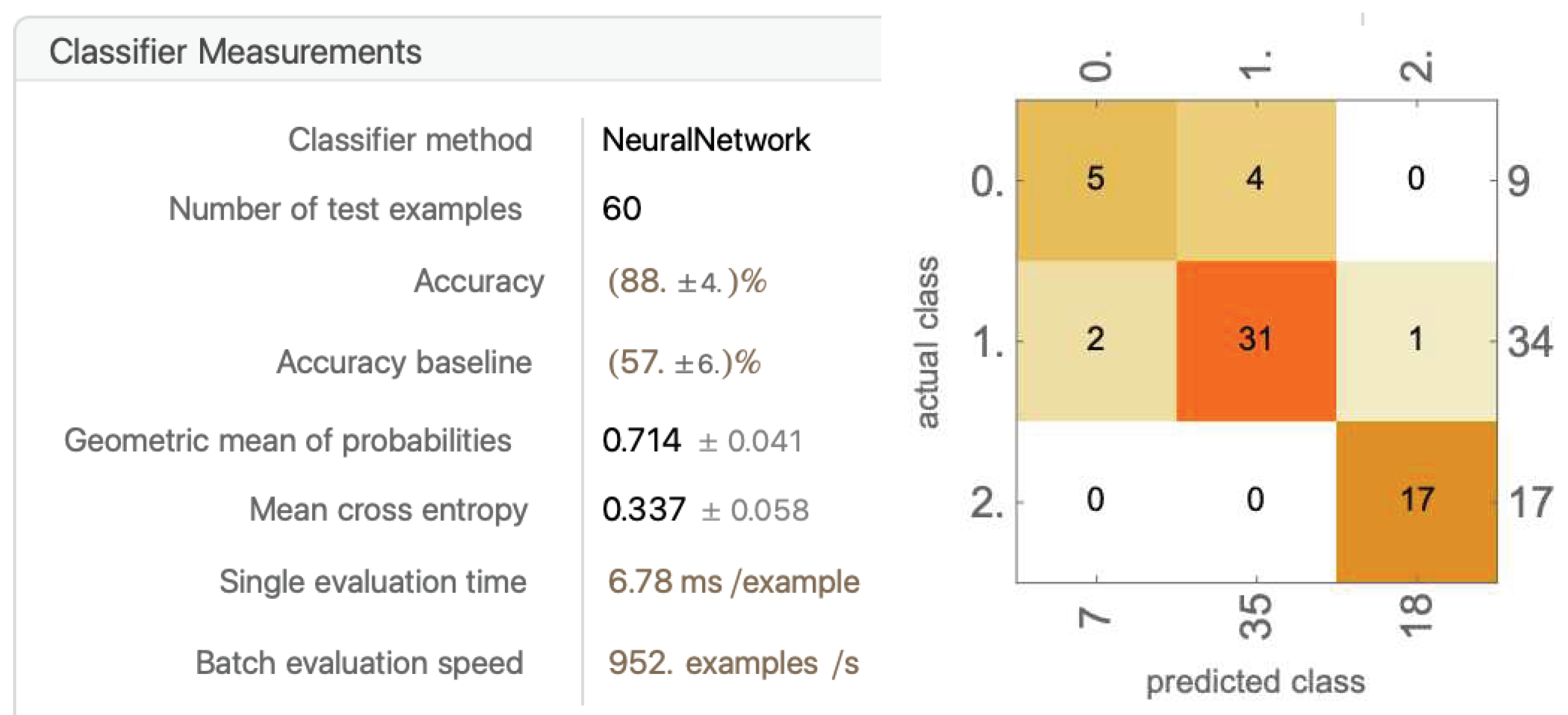
Overall, the five runs averaged an average accuracy of 81.4% ± 8.36%. The accuracy varies drastically over the five runs. The highest accuracy reached 95%, and the lowest fell down to 70%. Over the five runs, the distribution of the randomized data is relatively consistent: 8 No Lets, 33 to 36 Yes Lets, and 16 to 19 Strokes. The models are able to accurately classify Yes Lets, and are relatively able to accurately classify Strokes. Most models struggle with classifying No Lets.
Worth noting, in every model, the values of No Let being classified as stroke and stroke classified as No Lets are mostly zero, with the greatest not exceeding two. This shows that there is, in fact, a clear divide in Strokes and No Lets, and such a difference can be detected with the neural network.
4.1.2.2 Dropping Out Data Components
As only the positional values are inputted, some values may act as noise to the model and, in fact, cause the model to perform worse. We kept the AP position, the RP position, and the ball position in frame, then investigated the effect of dropping out combinations of the remaining values.
Figure 24.
A trial of the five models trained with dropping out racket head position (for remaining four trials, see Appendix B).
Figure 24.
A trial of the five models trained with dropping out racket head position (for remaining four trials, see Appendix B).
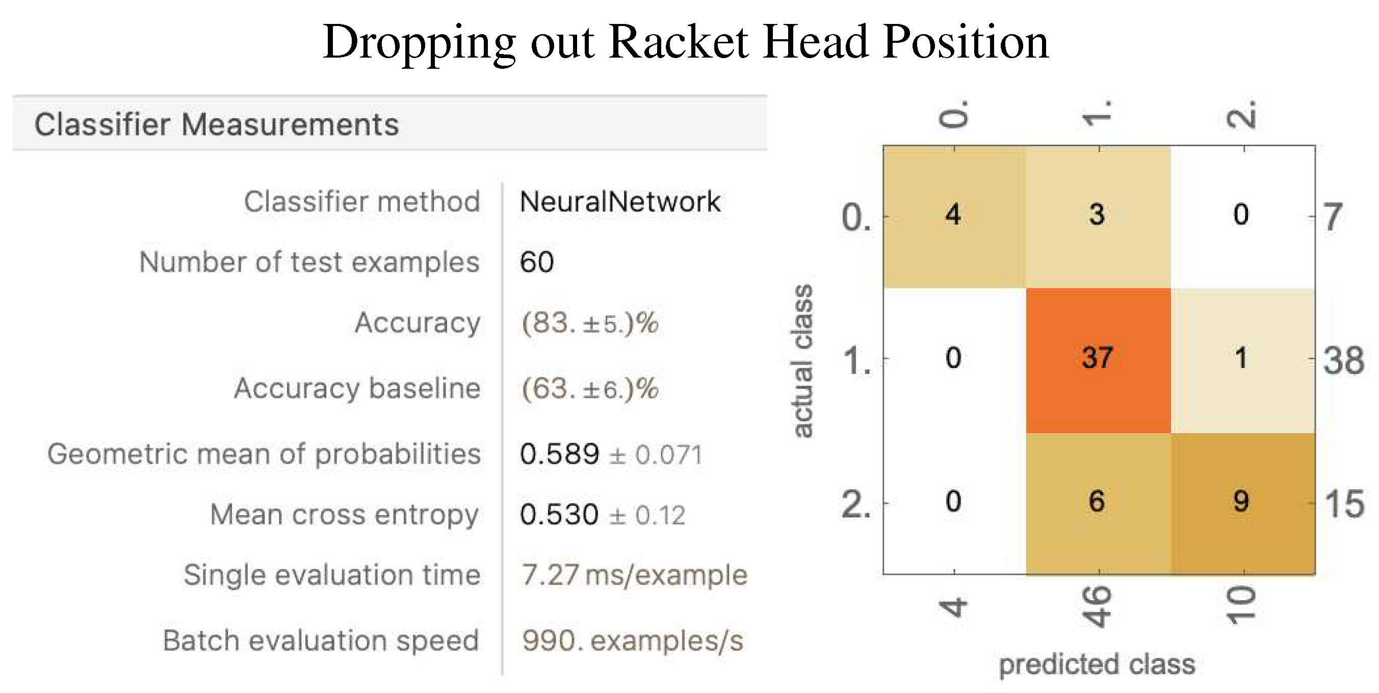
The result of dropping out the racket head position yielded an average accuracy of 82.6% ± 5.89%. The accuracy improved by 1%, and the standard deviation went down by nearly 3%. Over the few runs, the randomized dataset was less stable than when trained using six parameters, with more fluctuations in the amount of each decision. The Yes Lets and Strokes were still being classified with accuracy, and the No Lets were being classified with more consistent accuracy. The results confirmed the hypothesis that the model may perform better after dropping out some data components. The rationale behind this scenario could possibly be that the racket head position provides similar information as the AP position, just offset by the reach of the player. Thus, having similar information with noise may not help the model after all.
Dropping out Racket Head Position and the First Bounce Position
Figure 25.
A trial model trained with dropping out racket head position and the first bounce position (for remaining 4 trials, see Appendix C).
Figure 25.
A trial model trained with dropping out racket head position and the first bounce position (for remaining 4 trials, see Appendix C).
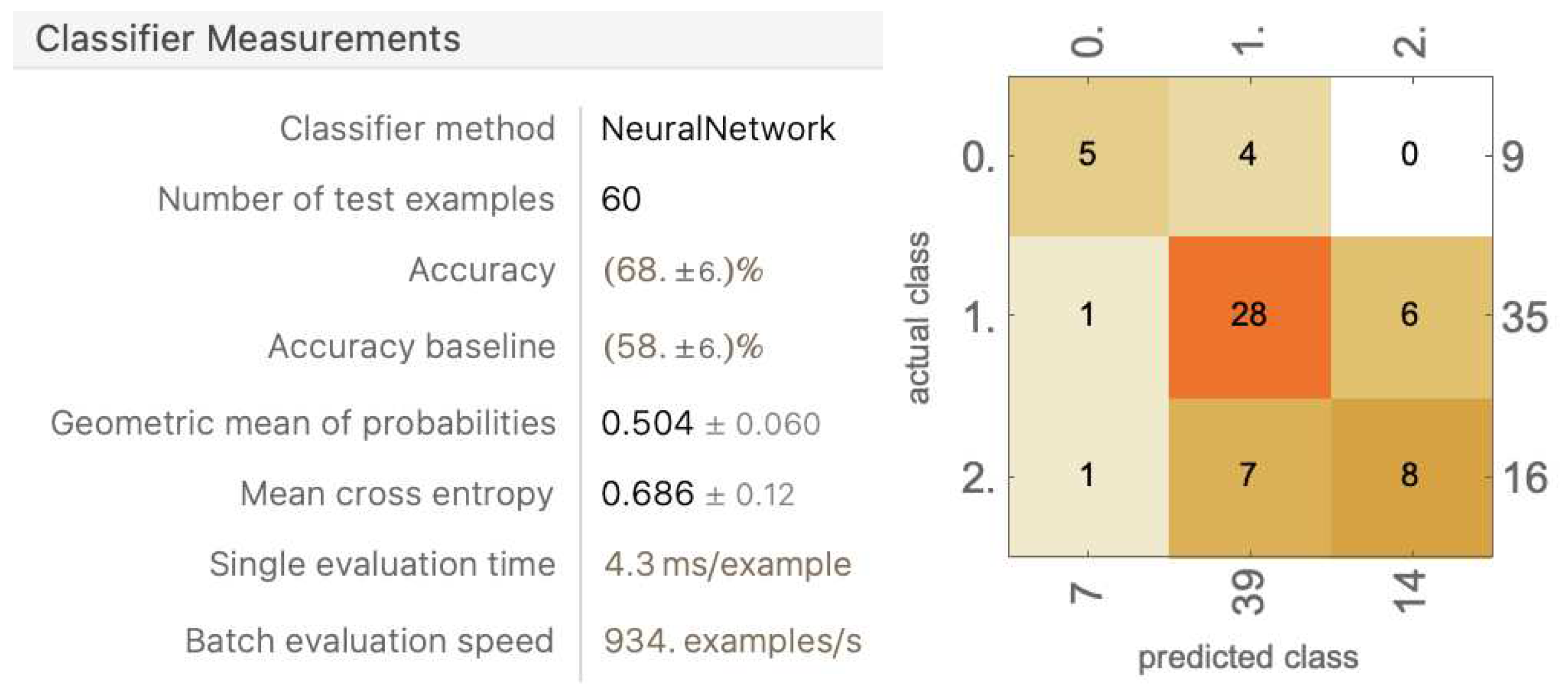
Removing the information of the first bounce position drastically decreased the model performance to an average accuracy of 71.6% ± 5.82%. The model became more inconsistent with every category compared to only dropping out racket head position. The first bounce position was removed, as we hypothesized that the ball position in frame and the second bounce could provide enough information about the ball’s path, and the first bounce position, sometimes located in front of the ball position in frame and sometimes located behind, will only provide a noise. This hypothesis was proven wrong, as the first bounce position does play an important role in predicting decisions.
Dropping out Racket Head Position and Second Bounce Position
Figure 26.
A trial model trained with dropping out racket head position and the second bounce position (for remaining 4 trials, see Appendix D).
Figure 26.
A trial model trained with dropping out racket head position and the second bounce position (for remaining 4 trials, see Appendix D).
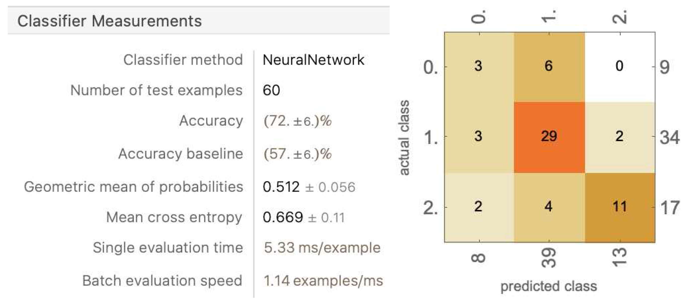
The models trained with these sets of data components performed the worst of all, with average accuracy falling below 69% ± 1.79%. The rationale behind taking away the second bounce is that, in all interferences, the contact happened before the second bounce, and in many interferences, the second bounce traveled away from the position of contact, which may have caused it to be less valuable as an informational data component. However, this notion has been proven wrong, as the accuracy fell below 70% and became inconsistent in all categories.
4.1.3. Model Performance with Modified Data Components
The nine modified data components are as follows:
Distance of Attacking Player (AP) to Retreating Player (RP)
Distance of Attacking Player to Ball Position in Frame
Distance of Retreating Player to Ball Position in Frame
Distance of Attacking Player to Second Bounce
Distance of Racket Head to Retreating Player
Distance of the Ball Position in Frame to Second Bounce
Distance of Racket Head to Ball Position in Frame
The Shortest Distance From Racquet Head to The Path of Ball
Access to the Front Wall: How Much is Blocked by the Other Player
We proposed to train a model using this second-layer of information to see if it improves our model performance. Considering that within those nine pieces of information, some may contain similar information to others, we will train several models with selected values and compare their performances.
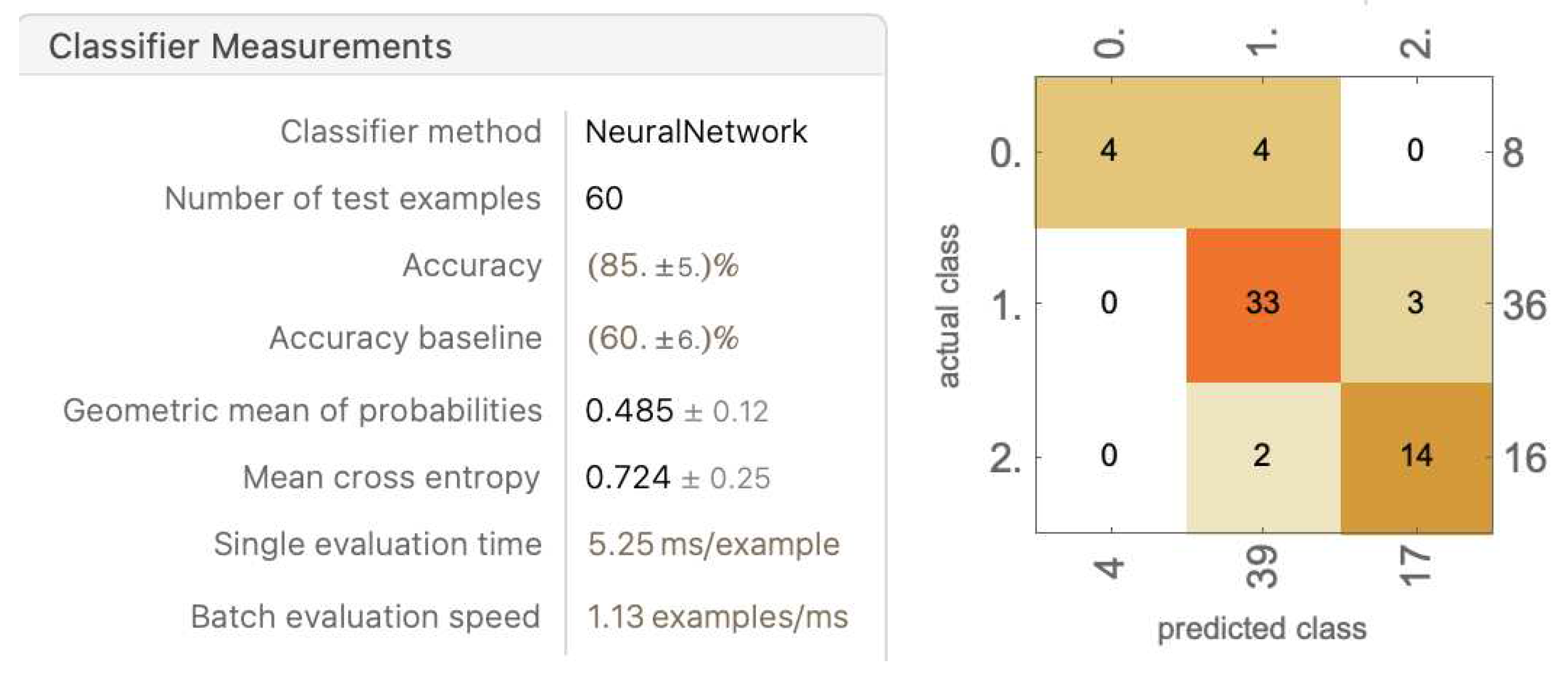
4.1.3.1. All Nine Modified Data Components (MDCs)
In this experiment, we used all nine MDCs to train the model. 340 decisions are used in the training set, and 60 are used in the testing set.
Figure 27.
A trial model trained on all nine modified data components (for remaining four trials, see Appendix E).
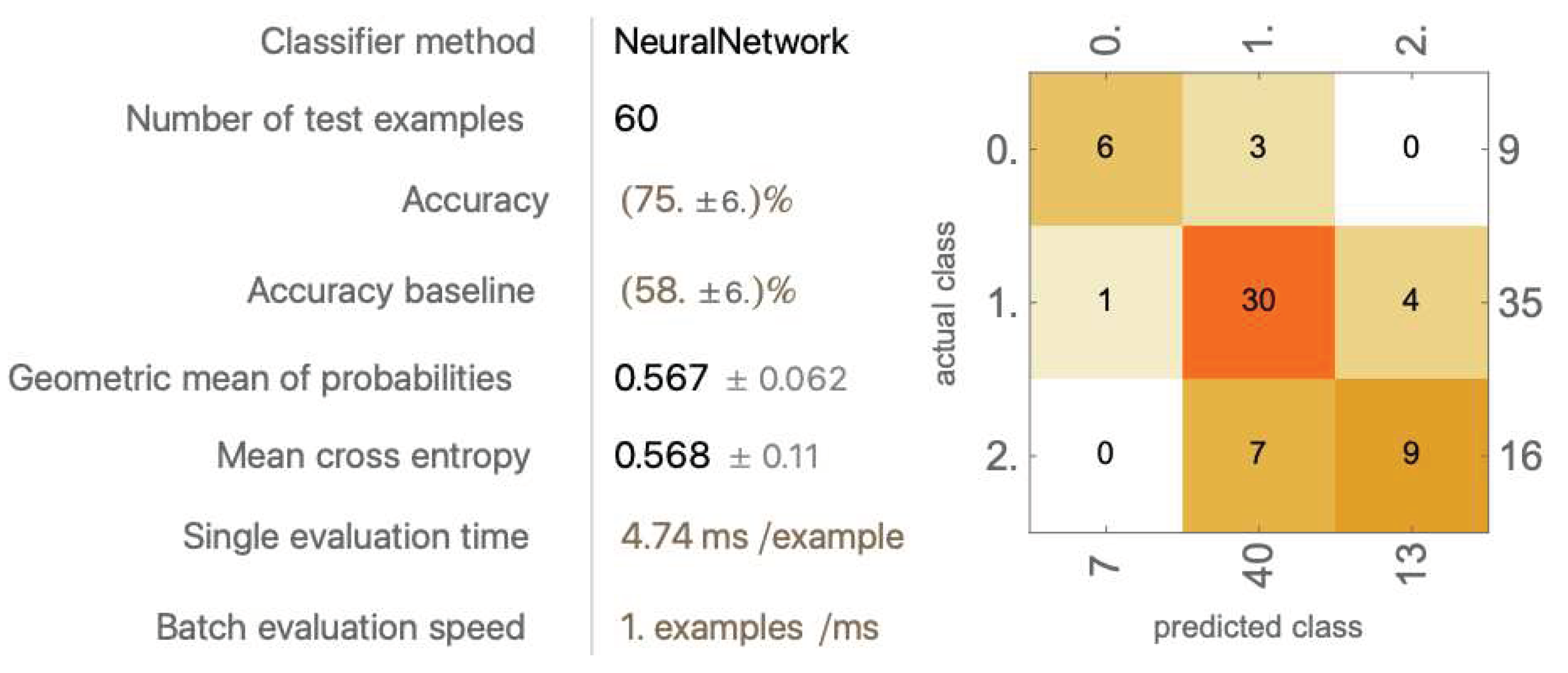
Figure 27.
A trial model trained on all nine modified data components (for remaining four trials, see Appendix E).
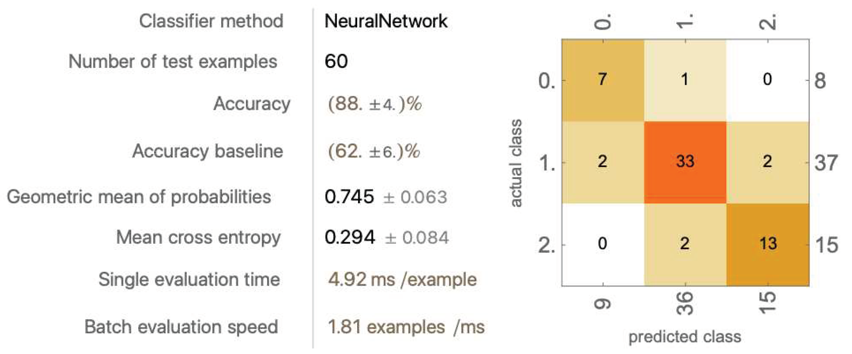
The average accuracy reached 86% ± 3.03%. This performance was the best model achieved yet through Wolfram Mathematica. Compared to the previous best model achieved by dropping out racket head position, the average accuracy improved by 3.4% and standard deviation decreased by 2.86%
4.1.3.2 Including Modified Data Components (MDCs) #1, #2, #3, #4, #6, #8, #9
In the second experiment, we excluded MDC #5 and MDC # 7 as we believe they can be redundant to some of the other values. MDC #5, “Distance of Racket Head to Retreating Player,” provides similar information to MDC #1, “Distance of Attacking Player to Retreating Player. ” MDC #7, “Distance of Racket Head to Ball Position in Frame,” provides similar information to MDC #4, “Distance of Attacking Player to Second Bounce.”
Figure 28.
A trial model trained on seven modified data components (for remaining four trials, see Appendix F).
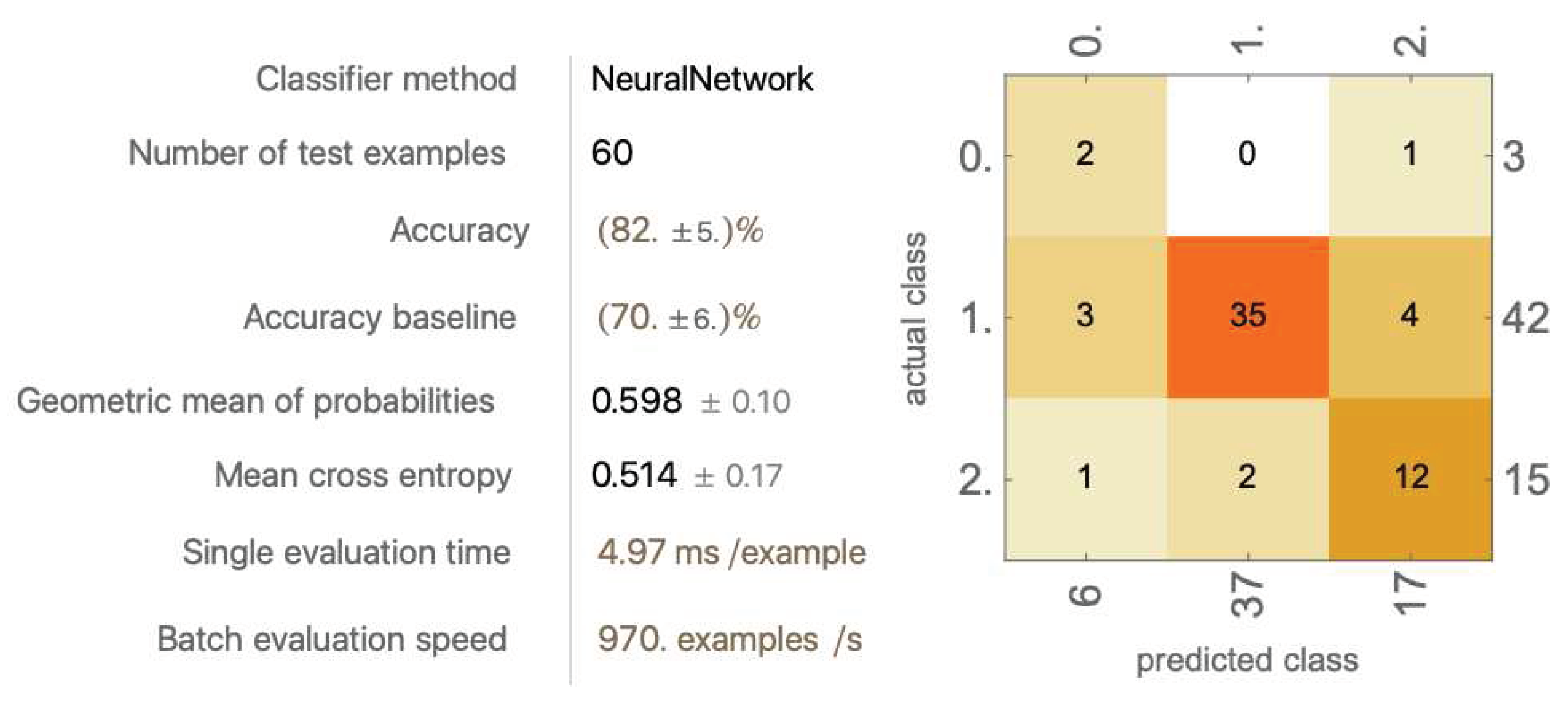
Figure 28.
A trial model trained on seven modified data components (for remaining four trials, see Appendix F).
The average accuracy dropped to 81.2% ± 6.625%. This indicates that this was a failed attempt to remove information. The standard deviation also drastically increased. Some trials reached an accuracy of 90%, yet some dropped to 73%. Overall, the results were inconsistent and the accuracy dropped.
4.1.3.3 Including Modified Data Components (MDCs) #1, #2, #3, #4, #6
In our third experiment, MDC #8 and MDC #9 were also removed. Those two values are two special cases because, in the process of calculating these values, complicated methods were used (see section 3.5.8 and 3.5.9). All other values were calculated simply by finding the distance between positions. In removing those two values we wanted to see how much they contributed to the model performance.
Figure 29.
A trial model trained on five modified data components (for remaining four trials, see Appendix G).
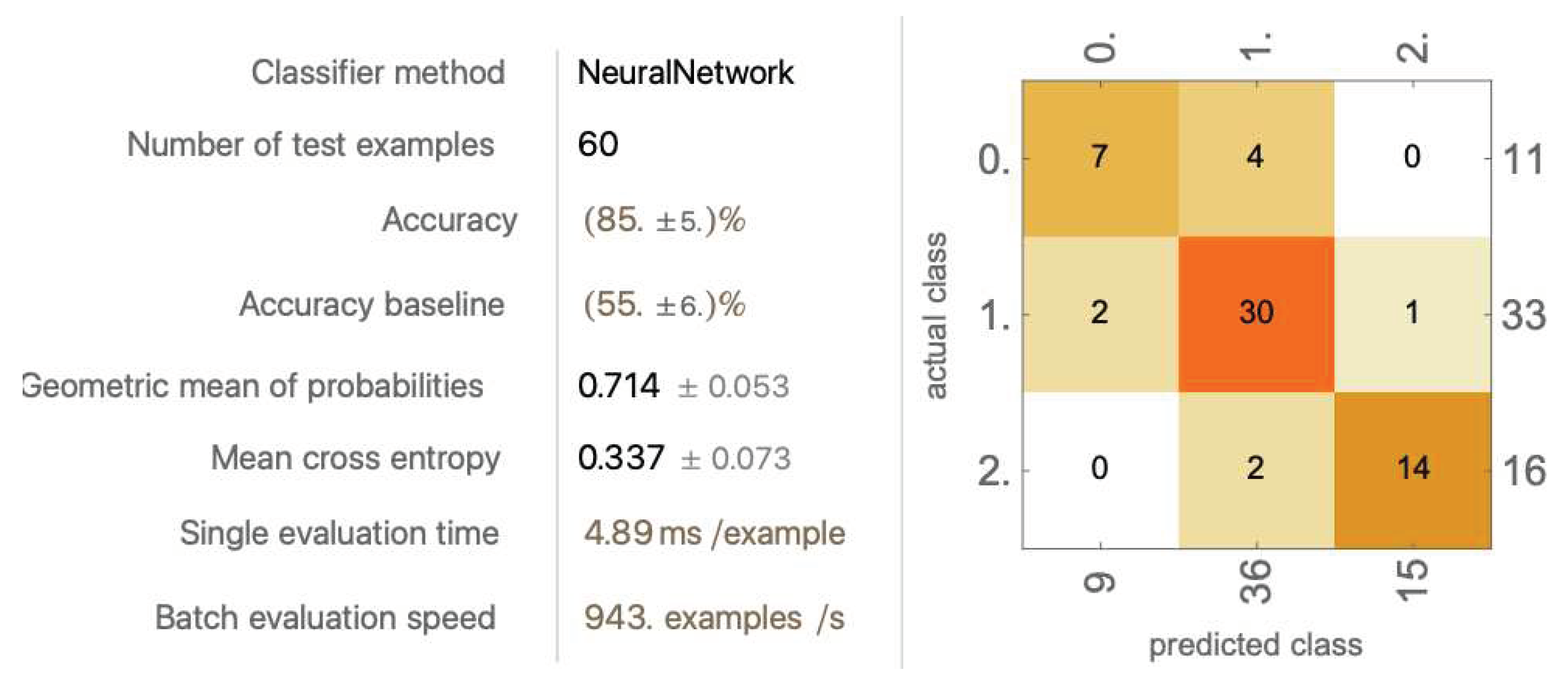
Figure 29.
A trial model trained on five modified data components (for remaining four trials, see Appendix G).
The model performance reached an average accuracy of 78.8 % ± 5.84 %. This value is more than 7% lower than when all nine MDCs were used and 2.4% lower than when only MDCs #5 and #7 were removed. This indicates that those two values indeed contain useful information for the model’s performance.
4.1.4. Model Performance with Modified Data Components Combined with Primitive Data Components
In this 4.1 section showing the Wolfram Mathematica results, we explored the performance of our model when trained with two sets of data components: the modified data components (MDCs) and the primitive data components (PDCs). The idea behind this is that although the distance-related data components, which are the modified data components, can provide a good insight of what the situation is, the model could not understand the location of where on the court this happened. Therefore, by combining the position-related data components and the distance-related data components, we can build a model that considers the situation in a more well-rounded way, which hopefully can increase the model performance.
There are, in total, 21 data components in consideration (12 Primitive and 9 Modified). In this section, combinations of each are going to be tested. All PDCs and MDCs are listed here.
PDCs:
1 & 2: Attacking Player Position X and Y Value
3 & 4: Retreating Player Position
5 & 6: Ball Position in the frame
7 & 8: First Bounce
9 & 10: Second Bounce
11 & 12: Racket Head Position
MDCs:
Distance of Attacking Player (AP) to Retreating Player (RP)
Distance of Attacking Player to Ball Position in Frame
Distance of Retreating Player to Ball Position in Frame
Distance of Attacking Player to Second Bounce
Distance of Racket Head to Retreating Player
Distance of Ball Position in Frame to Second Bounce
Distance of Racket Head to Ball Position in Frame
The Shortest Distance from Racquet Head to The Path of Ball
Access to the Front Wall: How Much is Blocked by the Other Player
4.1.4.1 Training with all 21 Data Components
In the first experiment, we utilize all data components we have. All 21 data components are fed into the model, and we investigated the model performance.
Figure 30.
A trial model trained on all 21 data components (for remaining four trials, see Appendix H).
Figure 30.
A trial model trained on all 21 data components (for remaining four trials, see Appendix H).
The model’s accuracy dropped to 81.8% ± 3.71%. Surprisingly, the model performance did not improve after combining the PDCs and the MDCs. One possible explanation for this is that too many data components were provided for a small dataset. The model is incapable of learning all the correlations using the resources it has.
4.1.4.2 Training with Primitive Data Components (PDCs) #1-10 and all Modified Data Components (MDCs)
As shown in previous experiments, including PDCs #11 and 12 (racket head position) acted as a noise to the model. In this experiment, we excluded those two values and evaluated the model performance.
Figure 31.
A trial model trained on primitive data components #1-10 and all modified data components (for remaining four trials, see Appendix I).
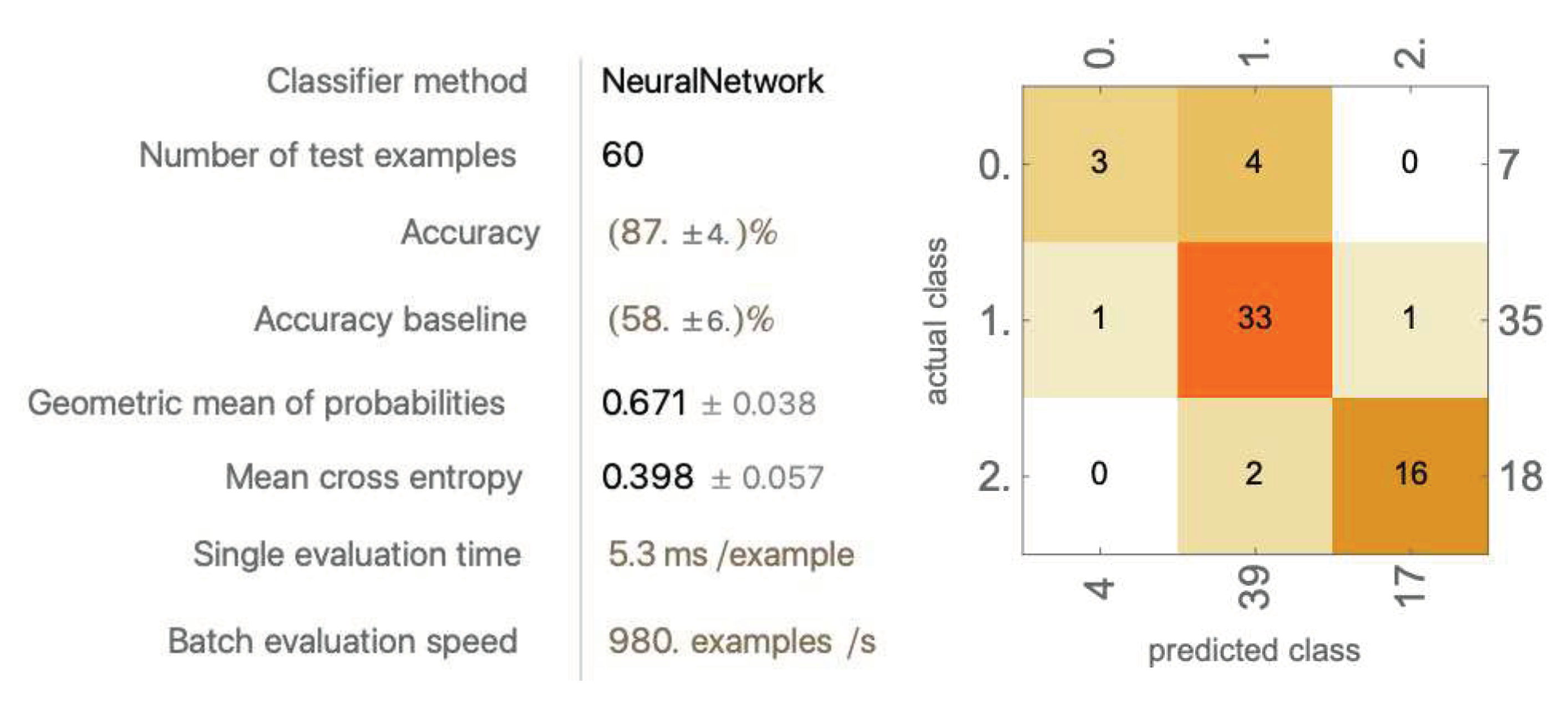
Figure 31.
A trial model trained on primitive data components #1-10 and all modified data components (for remaining four trials, see Appendix I).
The average accuracy is 82.2% ± 6.68%. No significant improvements are made after those values are removed.
4.1.4.3 Training with Primitive Data Components (PDCs) #1-10 and Modified Data Components (MDCs) #3, 5, 6, 8, and 9
In this experiment, we selected from MDC values and evaluated model performance.
Figure 32.
A trial model trained on primitive data components #1-10 and five modified data components (for remaining four trials, see Appendix J).
Figure 32.
A trial model trained on primitive data components #1-10 and five modified data components (for remaining four trials, see Appendix J).
The average accuracy reaches 84.8% ± 6.17%. No significant improvements are made after some values are removed.
4.2. Results with Python
4.2.1. Experimental Design
Slightly different from the method used with Wolfram Mathematica, the 400 decisions are split into three sections: 280 (70%) in the training set, 40 (10%) in the validation set, and 80 (20%) in the testing set. The neural network consists of two layers with 64 nodes and 128 nodes, and one output layer.
In the training process, the Pandas package is used to read the dataset. The Scikit-learn package is used to shuffle the dataset. The TensorFlow package is used to modify the data and train the neural network.
4.2.2. Model Performance on Primitive Data Components
4.2.2.1 Training on All Six Data Components

Table 1.
Five trials of the model trained on all six data components.
| Trial 1 | Trial 2 | Trial 3 | Trial 4 | Trial 5 | |
|---|---|---|---|---|---|
| Accuracy on the Test Set | 0.762 | 0.750 | 0.775 | 0.712 | 0.737 |
| Loss | 0.714 | 0.729 | 0.656 | 0.725 | 0.761 |
The models trained with all six data components performed significantly worse than their Wolfram Mathematica counterparts, achieving an average accuracy of 0.747 ± 0.022 and an average loss of 0.717 ± 0.034. With Wolfram Mathematica’s built-in neural network training method unavailable, it was hard to replicate the results achieved by Wolfram Mathematica.
4.2.2.2 Dropping Out Data Components
Although it is hard to replicate the results achieved by Wolfram Mathematica, the same drop-out method can be tested on the neural network. The core data components of AP Position, RP Position, and the ball position in frame are kept, and the remaining three are dropped to test if this method will increase the performance of the model.
Table 2.
Five trials of the model trained by dropping out the racket head position.
| Trial 1 | Trial 2 | Trial 3 | Trial 4 | Trial 5 | |
|---|---|---|---|---|---|
| Accuracy on the Test Set | 0.825 | 0.712 | 0.813 | 0.700 | 0.800 |
| Loss | 0.747 | 0.571 | 0.461 | 1.03 | 0.491 |
Average Accuracy: 0.77 ± 0.053; Average Loss: 0.66 ± 0.21
Table 3.
Five trials of the model trained by dropping out racket head position and second bounce position.
Table 3.
Five trials of the model trained by dropping out racket head position and second bounce position.
| Trial 1 | Trial 2 | Trial 3 | Trial 4 | Trial 5 | |
|---|---|---|---|---|---|
| Accuracy on the Test Set | 0.800 | 0.75 | 0.738 | 0.788 | 0.738 |
| Loss | 0.930 | 0.643 | 0.624 | 0.552 | 0.662 |
Average Accuracy: 0.763 ± 0.026; Average Loss: 0.682 ± 0.129
Table 4.
Five trials of the model trained by dropping out racket head position and first bounce position.
Table 4.
Five trials of the model trained by dropping out racket head position and first bounce position.
| Trial 1 | Trial 2 | Trial 3 | Trial 4 | Trial 5 | |
|---|---|---|---|---|---|
| Accuracy on the Test Set | 0.788 | 0.800 | 0.800 | 0.775 | 0.75 |
| Loss | 0.714 | 0.525 | 0.526 | 0.934 | 0.634 |
Average Accuracy: 0.783 ± 0.016; Average Loss: 0.667 ± 0.151
Table 5.
Five trials of the model trained by dropping out racket head position, first bounce position, and second bounce position.
Table 5.
Five trials of the model trained by dropping out racket head position, first bounce position, and second bounce position.
| Trial 1 | Trial 2 | Trial 3 | Trial 4 | Trial 5 | |
|---|---|---|---|---|---|
| Accuracy on the Test Set | 0.738 | 0.675 | 0.775 | 0.712 | 0.738 |
| Loss | 0.568 | 0.752 | 0.617 | 0.752 | 0.943 |
Average Accuracy: 0.728 ± 0.033; Average Loss: 0.726 ± 0.131
The model that achieved the best accuracy is the one trained on the dataset, which dropped out the racket head position and first bounce position, with an average accuracy of 78.3% ± 1.6%, around 4% less accurate than the best model trained in Wolfram Mathematica.
4.2.3. Model Performance and Normalization
Taking the best model (trained on dropping out the Racket Head Position and First Bounce Position), we investigated the effect of Normalization on this task. The above results were all performed by models trained with data normalized by TensorFlow’s built-in normalization function. We trained models five more times without the Normalization to see the result.
Table 6.
Five trials of the model trained without normalization.
| Trial 1 | Trial 2 | Trial 3 | Trial 4 | Trial 5 | |
|---|---|---|---|---|---|
| Accuracy on the Test Set | 0.625 | 0.712 | 0.712 | 0.825 | 0.712 |
| Loss | 0.849 | 0.679 | 0.733 | 0.59 | 0.714 |
Average Accuracy: 0.717 ± 0.064; Average Loss: 0.713 ± 0.084
The average accuracy dropped by around 7% with a similar average loss. This result demonstrates that the normalization method has helped the model during the classification process.
4.2.4. Model Performance with Modified Data Components
The nine modified data components are as follows:
Distance of Attacking Player (AP) to Retreating Player (RP)
Distance of Attacking Player to Ball Position in Frame
Distance of Retreating Player to Ball Position in Frame
Distance of Attacking Player to Second Bounce
Distance of Racket Head to Retreating Player
Distance of Ball Position in Frame to Second Bounce
Distance of Racket Head to Ball Position in Frame
The Shortest Distance From Racquet Head to The Path of Ball
Access to the Front Wall: How Much is Blocked by the Other Player
We proposed to train a model using this second-layer of information to see if it will improve our model performance. Considering that within those nine pieces of information, some may contain similar information with another, we will train several models with selected values and compare their performances.
4.2.4.1 All Nine Modified Data Components (MDCs)
In the first experiment of this section, we decided to use all nine values to train the model. The experimental parameters were kept the same, with 280 decisions in the training set, 40 in the validation set, and 80 in the testing set. The neural network still consists of two layers with 64 nodes, 128 nodes, and one output layer.
Table 7.
Five trials of the model trained with all nine modified data components.
| Trial 1 | Trial 2 | Trial 3 | Trial 4 | Trial 5 | |
|---|---|---|---|---|---|
| Accuracy on the Test Set | 0.825 | 0.837 | 0.762 | 0.774 | 0.825 |
| Loss | 0.685 | 0.374 | 0.430 | 0.615 | 0.603 |
Average Accuracy: 0.805 ± 0.030, Average Loss 0.541 ± 0.119
Our model reached an accuracy of 80.5% ± 3.0%. This result exceeded the previous best model achieved in Python by around 1.7% on average. The average loss drastically decreased by more than 15%. This indicates that the modified data approach may indeed be useful to the model training process.
4.2.4.2 Including Modified Data Components (MDCs) #1, #2, #3, #4, #6, #8, #9
In the second experiment, we excluded MDC #5 and MDC # 7. These two values are excluded as we believe they can be redundant to some of the other values. MDC #5, “Distance of Racket Head to Retreating Player,” provides similar information to MDC #1, “Distance of Attacking Player to Retreating Player.” MDC #7, “Distance of Racket Head to Ball Position in Frame,” provides similar information to MDC #4, “Distance of Attacking Player to Second Bounce.”
Table 8.
Five trials of the model trained with seven modified data components.
| Trial 1 | Trial 2 | Trial 3 | Trial 4 | Trial 5 | |
|---|---|---|---|---|---|
| Accuracy on the Test Set | 0.813 | 0.800 | 0.775 | 0.813 | 0.850 |
| Loss | 0.557 | 0.538 | 0.421 | 0.535 | 0.985 |
Average Accuracy: 0.810 ± 0.024, Average Loss 0.607 ± 0.195
The average accuracy increased by 0.5%, indicating that this was a successful attempt of removing information. The average loss stayed around the same value, increasing by 6%.
4.2.4.3 Including Modified Data Components (MDCs) #1, #2, #3, #4, #6
In our third experiment, MDC #8 and MDC #9 were removed. Those two values are two special cases, because in the process of calculating those values, complicated methods were used (see section 3.5.8 and 3.5.9). All other values were calculated by finding the distance between positions. In removing those two values, we wanted to see how much they contributed to the model performance.
Table 9.
Five trials of the model trained with five modified data components.
| Trial 1 | Trial 2 | Trial 3 | Trial 4 | Trial 5 | |
|---|---|---|---|---|---|
| Accuracy on the Test Set | 0.775 | 0.75 | 0.887 | 0.762 | 0.850 |
| Loss | 0.573 | 0.530 | 0.353 | 0.528 | 0.545 |
Average Accuracy: 0.805 ± 0.054, Average Loss 0.505 ± 0.078
Surprisingly, the model accuracy did not drop compared to using all nine data components. The model also has a lower and comparatively more stable standard deviation. This might indicate that MDCs #8 and #9 do not provide extremely useful information.
4.2.5. Model Performance with Modified Data Components combined with Primitive Data Components
In this 4.2 section showing the Python results, we explored the performance of our model when trained with two sets of data: the modified data components (MDCs) and the primitive data components (PDCs). The idea behind this is that although the distance-related data components, which are the modified data components, can provide a good insight of what the situation is, the model could not understand the location of where on the court this happened. Therefore, through combining the position-related data components and the distance-related data components, we can build a model that considers the situation in a more well-rounded way, which hopefully can increase the model performance.
There are, in total, 21 data components in consideration (12 primitive and 9 modified). In this section, combinations of each are going to be tested. All PDCs and MDCs are listed here.
PDCs:
1 & 2: Attacking Player Position X and Y value
3 & 4: Retreating Player Position
5 & 6: Ball Position in the frame
7 & 8: First Bounce
9 & 10: Second Bounce
11 & 12: Racket Head Position
MDCs:
Distance of Attacking Player (AP) to Retreating Player (RP)
Distance of Attacking Player to Ball Position in Frame
Distance of Retreating Player to Ball Position in Frame
Distance of Attacking Player to Second Bounce
Distance of Racket Head to Retreating Player
Distance of Ball Position in Frame to Second Bounce
Distance of Racket Head to Ball Position in Frame
The Shortest Distance From Racquet Head to The Path of Ball
Access to the Front Wall: How Much is Blocked by the Other Player
4.2.5.1 Training with all 21 data Components
In the first experiment, we utilized all data components we have. All 21 data components were fed into the model, and we investigated the model performance.
Table 10.
Five trials of the model trained with all 21 data components.
| Trial 1 | Trial 2 | Trial 3 | Trial 4 | Trial 5 | |
|---|---|---|---|---|---|
| Accuracy on the Test Set | 0.850 | 0.813 | 0.837 | 0.850 | 0.837 |
| Loss | 0.562 | 1.32 | 0.561 | 0.425 | 0.547 |
Average Accuracy: 0.837 ± 0.014, Average Loss: 0.683 ± 0.323
The model achieved the highest accuracy yet in the Python section, exceeding the previous best Python model by 2.7%. This proves the idea that positional data components, adding to the distance-related data components, can improve the model’s understanding of interferences and thereby improve its performance.
4.2.5.2 Training with Primitive Data Components (PDC) 1-10 and all Modified Data Components (MDCs)
As shown in previous experiments, PDCs #11 and 12 (racket head position) could act as a noise to the model. In this experiment, we excluded those two values and evaluated the model performance.
Table 11.
Five trials of the model trained with primitive data componentss #1 - #10 and all modified data components.
Table 11.
Five trials of the model trained with primitive data componentss #1 - #10 and all modified data components.
| Trial 1 | Trial 2 | Trial 3 | Trial 4 | Trial 5 | |
|---|---|---|---|---|---|
| Accuracy on the Test Set | 0.875 | 0.762 | 0.875 | 0.837 | 0.912 |
| Loss | 1.39 | 0.764 | 0.319 | 0.399 | 0.252 |
Average Accuracy: 0.852 ± 0.051, Average Loss: 0.625 ± 0.421
In this experiment, the average accuracy once more experienced a considerable improvement of around 1.5% over the model trained in the last experiment. It is currently the model with the best accuracy in the Python section. Worth noting, the fifth trial provided the current best singular trial model in Python with 91.2% accuracy.
4.2.5.3 Training with Primitive Data Components (PDCs) #1-10 and Modified Data Components (MDCs) #3, 5, 6, 8, and 9
In this experiment, we selected from MDC values and evaluated model performance.
Table 12.
Five trials of the model trained with primitive data components #1 - 10 and five modified data components.
Table 12.
Five trials of the model trained with primitive data components #1 - 10 and five modified data components.
| Trial 1 | Trial 2 | Trial 3 | Trial 4 | Trial 5 | |
|---|---|---|---|---|---|
| Accuracy on the Test Set | 0.875 | 0.813 | 0.837 | 0.850 | 0.875 |
| Loss | 0.466 | 0.760 | 0.472 | 0.424 | 0.364 |
Average Accuracy: 0.850 ± 0.024, Average Loss: 0.497 ± 0.137
Compared to the last model, this model achieved 85% accuracy (within 0.2% of the last model) with far better loss. The loss is 12% lower than the previous model with a far steadier standard deviation.
5. Discussion
5.1. Analysis of Result
In this section, we analyze the results we found in the study. We compared the best results from both Python and Mathematica.
5.1.1. Overall Result
Overall, the best model by Wolfram Mathematica performed an average accuracy of 86% ± 3.03%; the best model by Python performed an average accuracy of 0.852 ± 0.051 (which is 85.2% ± 5.1%).
An average accuracy of 85% already reaches the level of satisfaction in a real-life setting. For instance, in a regular professional match, the number of calls can vary between 20 to 30. If 85% of the decisions are made correctly, only three to five decisions are going to be incorrectly made. Given that, in many cases, an interference can be called either way (No Let or Yes Let, Yes Let or Stroke), referees nowadays already make almost three controversial calls in a regular match.
On the other hand, although the best models from Wolfram Mathematica and Python have similar average accuracies, they were trained using drastically different data components. In Wolfram Mathematica, the best model was achieved using only the nine modified data components. In Python, the best model was achieved using both the 9 modified data components (MDCs) and the primitive data components (PDCs) #1 - 10. This result indicates that models trained on different platforms vary in performance using the same data components. Wolfram Mathematica’s models dropped in accuracy when both PDCs and MDCs were used, but Python’s models peaked using these sets of data components.
After all, we do not have enough knowledge as to how Wolfram Mathematica’s neural networks are structured. This blind spot prevents us from being able to analyze why the two platforms vary in performance using the same sets of data components.
5.1.2. Usefulness of Different Data Components
To some extent, this study is an investigation into how different combinations of data components contribute to the model performance. Different combinations cause the models to perform differently, and their effects vary between the Wolfram Mathematica section and the Python Section.
The six primary data components (PDCs) already provide enough information for the model to perform at an acceptable level. Using only the six PDCs, the Wolfram Mathematica models reached an average accuracy of 81.4% ± 8.36%. The Python models reached a lower average accuracy of 74.7% ± 2.2% (0.747 ± 0.022).
The initial drop-out method removes different data components and evaluates the impact of those data components being removed. For Wolfram Mathematica, the accuracy increased to 82.6% ± 5.89% after the racket head position was removed. The accuracy drastically dropped after any other values were removed. For Python, the accuracy increased the most when both the racket head position and the first bounce position were removed, reaching 78% ± 1.6% (0.783 ± 0.016). The increase in performance after the removal of data components indicates that for the initial six data components, some contain information that could act as noise and actually stop the model from improving.
Then, the nine modified data components (MDCs) were introduced to the dataset. We conducted one round of experiments using only the nine MDCs and evaluated the models. Wolfram Mathematica’s models provided the best performance at this stage, reaching an average accuracy of 86% ± 3.03%. The Python models also experienced an increase in performance, reaching an average accuracy of 80.5% ± 3.0% (0.805 ± 0.030). This shows that the nine MDCs do, in fact, provide very useful information, and we were right in calculating the MDCs.
As some MDCs are slightly redundant, we experimented with data component drop-out on the nine MDCs. In the first round, MDCs #5 and #7 were removed. This dropped the Wolfram Mathematica models’ average accuracy to 81.2% ± 6.625% but increased the Python model’s average accuracy to 81.0% ± 2.4% (0.810 ± 0.024). In the second round, MDCs #8 and #9 were removed to evaluate their usefulness to our model, and for both platforms, the accuracy decreased, indicating that those two values are helpful to the model’s performance.
We then combined the MDCs and the PDCs to do a final round of evaluation. In this section, only the Python models have gained accuracy and better performance. When all MDCs and PDCs were used, the Python models achieved an average accuracy of 83.7% ± 1.4% (0.837 ± 0.014). When all MDCs and PDCs #1 - #10 were used, the Python models achieved their best performance of an average accuracy of 85.2% ± 5.1% (0.852 ± 0.051). Another combination of data components using MDCs #3, #5, #6, #8, #9 and PDCs #1 - #10 reached an average accuracy of 85.0% ± 2.4% (0.850 ± 0.024), with 15% less loss and far steadier standard deviation compared to the best-performing model.
5.2. Case-by-case Analysis of Some Wrong Calls
In this section, we performed a case-by-case analysis of incorrectly made decisions. We take two of each kind of incorrect decision made by our models and provide reasons as to why this might be incorrectly called in the model’s perspective and in the real-life perspective. We hope that in doing this, we can find some insights regarding why the model made the wrong calls.
The incorrect decisions are made by the best-performing models in Python. We chose models trained in Python for this section because the prediction results were easier to fetch, and the Python best-performing model was trained using PDCs #1 - #10 and all MDCs, thus, almost all data components were considered.
5.2.1. Yes Lets Classified Incorrectly
Figure 33.
Data #144, Matthew/Willstrop 2010 Canary Wharf 8:39 Yes Let [28]. Possibility given by model: [No Let - 94%, Yes Let - 6%, Stroke - 0% ].
Figure 33.
Data #144, Matthew/Willstrop 2010 Canary Wharf 8:39 Yes Let [28]. Possibility given by model: [No Let - 94%, Yes Let - 6%, Stroke - 0% ].
In this situation, the RP played a ball that died very quickly. The AP was provided a line to the ball. The referee deemed this situation a Yes Let, as interference happened and he thought that the AP could get the ball. From our perspective (as a non-professional normal viewer biased by our experiences), this could also be identified as a No Let, as the ball’s quality is high, and the AP may not be able to get the ball even without the interference.
The model deemed this more likely a No Let, possibly because the ball stayed up short. Worth noting, the possibility it provided is overwhelmingly in favor of the No Let decision, which should not be correct. The possibility for No Let should not reach more than 90%, as this case would be a close call.
Figure 34.
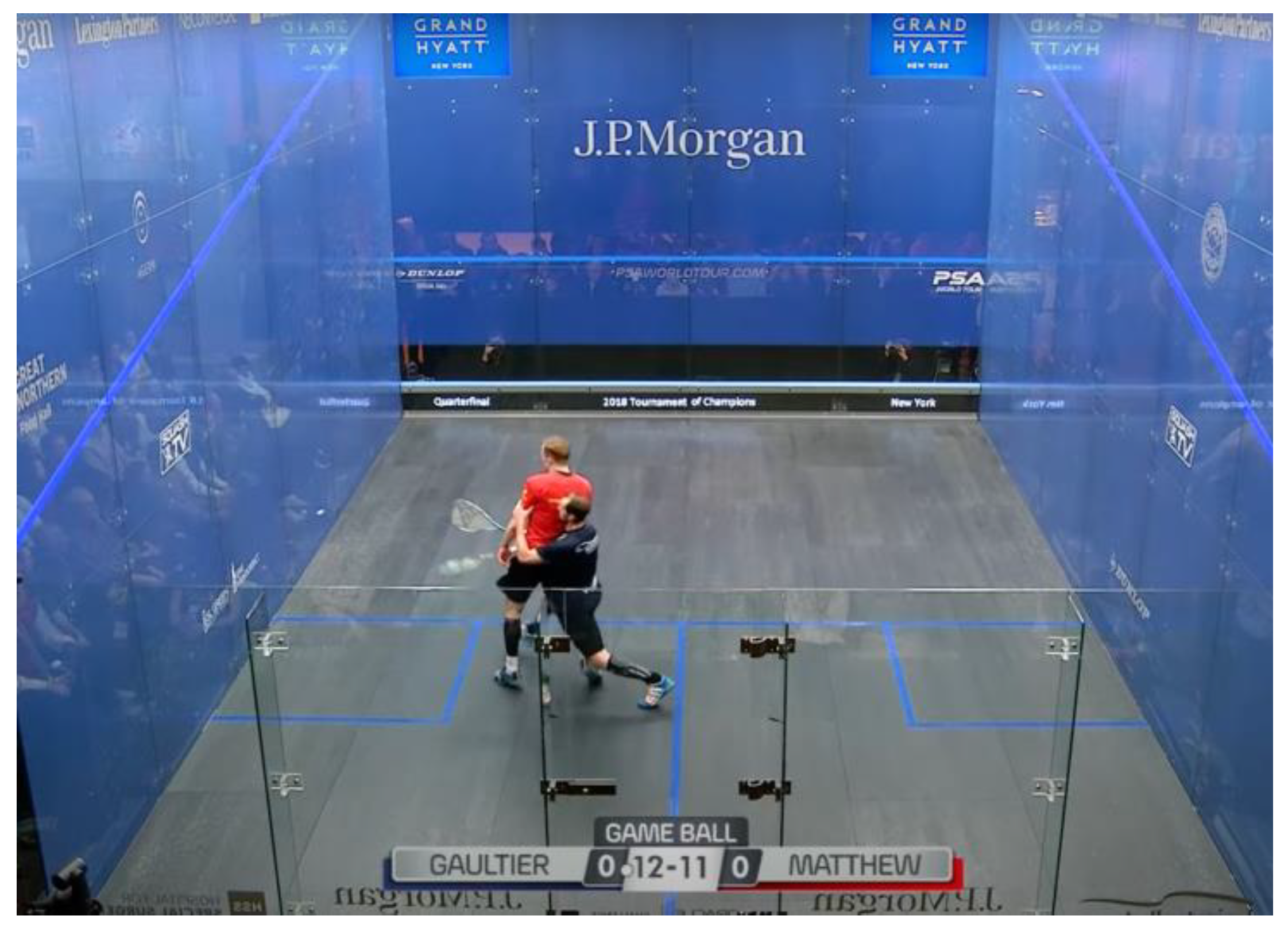
Data #347, Matthew/Gaultier 2018 ToC 1:32:33 Yes Let [34]. Possibility given by model: [No Let - 0%, Yes Let - 43%, Stroke - 57%].
Figure 34.
Data #347, Matthew/Gaultier 2018 ToC 1:32:33 Yes Let [34]. Possibility given by model: [No Let - 0%, Yes Let - 43%, Stroke - 57%].
This case, in fact, is a controversial case in itself. The RP played a ball that landed very close to him, yet the referee thinks there is enough distance away from it to be considered a Yes Let. In the video, the commentators pointed out that this case could well be a Stroke:
“Well, I mean eh, it's not the best of shots here from Matthew (the RP). This is going to be interesting, Massarella (the referee) is gotta be consistent… If you watch where the ball bounces, the second bounce is by the service line…. Well, I can assure you that Gregory Gaultier (the AP) will not be taking John Massarella out for any type of food or beverage… I think that was a stroke” [42].
Similar to the commentators, we think that this should be decided as a Stroke, because the ball bounced right back to the RP and the RP was not able to clear. Our model agreed with us by giving 57% of the possibility to Stroke. This provides a good example of how human referees can make controversial decisions that the commentators and the audiences disagree with.
5.2.2. No Lets Classified Incorrectly
Figure 35.
Data #46, Matthew/Elshorbagy 2014 British Open 1:03:19 No Let [25]. Possibility given by model: [No Let - 6%, Yes Let - 93%, Stroke - 0% ].
Figure 35.
Data #46, Matthew/Elshorbagy 2014 British Open 1:03:19 No Let [25]. Possibility given by model: [No Let - 6%, Yes Let - 93%, Stroke - 0% ].
This is not a very controversial decision. The RP’s shot went backward and was very tight to the side wall. Although the AP could have possibly retrieved the shot had the RP not been there, the AP first went the wrong way (forwards) as he was deceived by the shot. The AP also showed very little effort to go through the interference and play the ball. The AP took the “wrong path” to the ball, combined with the quality of the shot from RP and the AP’s lack of effort, which is why the referee deemed this a No Let.
Since our model has not learned the idea of “wrong path” and “effort,” it makes sense that it is unable to understand this situation. From the same position shown in the picture, if the AP took the “right path,” which is left and backward around the RP, this could well be decided as a Yes Let.
Figure 36.
Data #333, Matthew/Gaultier 2018 ToC 36:22 No Let [34].Possibility given by model: [No Let - 32%, Yes Let - 68%, Stroke - 0% ].
Figure 36.
Data #333, Matthew/Gaultier 2018 ToC 36:22 No Let [34].Possibility given by model: [No Let - 32%, Yes Let - 68%, Stroke - 0% ].
This case is a situation between a Yes Let and a No Let. The referee deemed the AP unable to reach the shot as the shot quality was “too good.”
In our opinion (as non-professional normal viewers biased by our experiences), this could be decided either way. Personally, we think that the AP might have been able to reach the ball had the RP provided a path, therefore, this could be decided as a Yes-Let. The commentators and the referee think the opposite because the ball’s quality was very good.
Our model, in fact, reflects our thinking by only providing a 32% possibility to No Let. This means that to the model, this could possibly be determined a No Let as well, although the model thinks that this situation is more towards a Yes Let.
After all, our model is trained with only 59 cases of No Let. This limits the amount of knowledge our model is able to learn, and it makes sense that our model is still unable to perform the most accurate refereeing.
5.2.3. Strokes Classified Incorrectly
Figure 37.
Data #46, Matthew/Elshorbagy 2014 British Open 58:10 Stroke [25]. Possibility given by model: [No Let - 0%, Yes Let - 53%, Stroke - 47%].
Figure 37.
Data #46, Matthew/Elshorbagy 2014 British Open 58:10 Stroke [25]. Possibility given by model: [No Let - 0%, Yes Let - 53%, Stroke - 47%].
This is a really interesting case. In this case, the AP is actually “fishing” for a Stroke. This means that the AP is manipulating his body position and exaggerating his swing to make the situation look more like a Stroke than a Yes Let. In this case, the AP stood his ground and waited for the ball instead of looking to play it normally. If the AP was going to play it normally, he would step into the ball and strike. Since he decided to fish for a Stroke, he shapes up and waits until the ball comes to him, as if he was going to hit the ball from where he is. This pushed the striking spot way back, which brought the RP into the range of the AP’s swing. This, combined with the AP’s exaggerated swing, makes the situation look more like a stroke. In reality, when the ball reaches him, it has already second-bounced, so he could not have hit it from where he is.
The commentators commented on the AP’s actions: “He (the AP) is looking for Shorbagy (the RP) there…Well, he’s got it (the Stroke), he is playing the rules…He (the AP) doesn’t usually do that, he doesn’t usually exaggerate. He is doing that (exaggerating his swing)” [46].
In this case, the referee gave a Stroke, although the AP is slightly fishing. In our understanding, the AP’s fishing actions changed the situation from a 50% Stroke to a 70% Stroke.
Our Model deemed this almost a fifty-fifty situation. Of course, there is no knowledge that informs the model that the AP is fishing for a Stroke. It makes sense that our model is deciding this slightly towards a Yes Let situation.
Figure 38.
Data #244, Ashour/Elshorbagy 2014 World Championship 12:08 Stroke [35]. Possibility given by model: [No Let - 0%, Yes Let - 51%, Stroke - 49%].
Figure 38.
Data #244, Ashour/Elshorbagy 2014 World Championship 12:08 Stroke [35]. Possibility given by model: [No Let - 0%, Yes Let - 51%, Stroke - 49%].
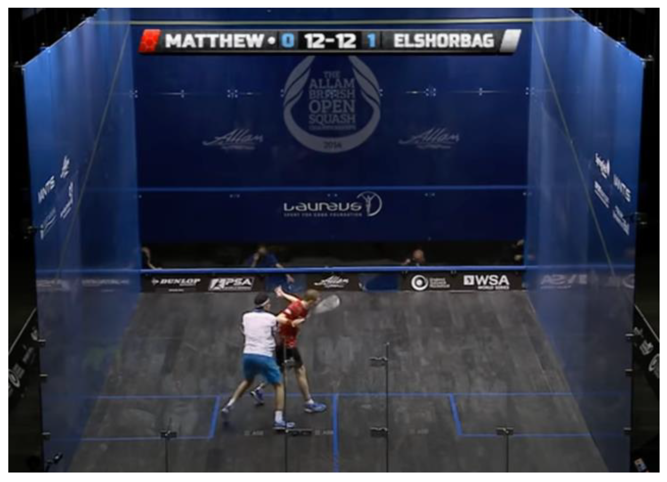
This is a pretty clear Stroke. The AP’s swing was prevented by the RP, and the ball was going right into the AP’s range of swing. The model made the wrong decision, possibly because the ball was at the front of the court when the interference happened, but it did not know that the ball was traveling really fast, and it entered AP’s range when the interference was still happening.
The model provided a 51% to 49% chance in favor of a Yes Let. These are two close possibilities, and with a slight change of one data component, this could possibly be overturned to a Stroke. This shows that our model is not far off in its predictions.
5.3. Limitations
5.3.1. Limitations in the Data Collection Process
5.3.1.1 Dataset is Too Small
The most glaring limitation of this study is the limited dataset. As there is no available dataset regarding squash refereeing decisions, we had to collect our own. Due to the limited time and resources, only 400 data were collected. The dataset is also severely imbalanced, with 243 Yes Lets but only 59 No Lets and 98 Strokes. If more data were provided, our model would be able to have more knowledge and almost surely going to perform significantly better in its tasks.
5.3.1.2. Speed and Height of The Ball
In our data collection process, we did not collect data components related to the speed and the height of the ball. However, those two data components can provide critical information about what a decision should be. With similar positioning and different speed and height of the ball, the decision could change from a Stroke to a No Let.
Figure 39.
Illustration of how balls with different speeds and heights can have the same first and second bounce positions.
Figure 39.
Illustration of how balls with different speeds and heights can have the same first and second bounce positions.
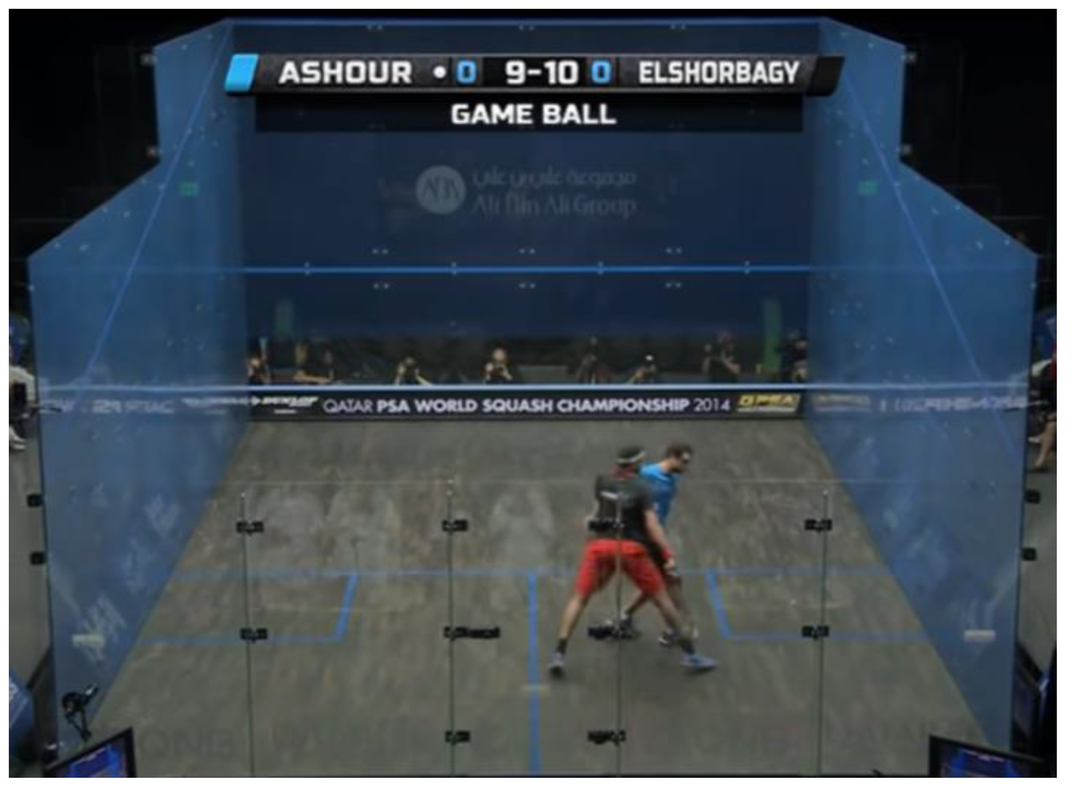
As shown in Figure 39, two shots can land in the same position, but the implications can differ drastically. The green path is a slow shot that could be easily retrieved, but the purple path is low and hard to retrieve. Without these two pieces of information, our model cannot learn the difference between the green path and the purple path.
5.3.1.3. Assumed All Decisions are Correct
During our data collection process, we had assumed all decisions we took in were correct decisions. However, some of them still are controversial (Data #347, see second example of 5.2.1). Our model is currently trained using some controversial data, which may have negatively influenced the model performance. If this issue is to be resolved, we need more than one squash professional discussing what each decision should be before putting the data into the dataset.
5.3.1.4. Took in Different Standards of Refereeing
Different referees have different standards of refereeing. Some referees are relatively soft, giving more Yes Lets on ambivalent cases. Some referees are harsh and give more Strokes and No Lets. The data collected for this study came from multiple referees, each having an individual system of refereeing. This leads to some similar cases in our dataset being classified as different decisions. One way to solve this is, like the possible resolution to 5.3.1.3, to have several squash professionals decide on one correct decision using one standard of refereeing during the process of data collection.
5.3.1.5. Different Definition of “Moment”
To collect our data, we defined a “moment,” which is the frame when the players first collide or when the ball first enters the AP’s range of swing. However, it is not always obvious when the moment is. Therefore, throughout the dataset, there are slight inconsistencies in the picking of moments.
5.3.1.6. When the Ball Bounces Off the Back Wall
When a ball travels deep and bounces off the back wall, it gives the AP more time to retrieve the wall. Most of the time, if the ball bounces off the back wall, the situation is not considered No Let. In our dataset, we did not put in a measure for when the ball bounced off the back wall. Simply noting down the second bounce of the ball does not tell the model if the ball has reached the back wall and bounced back, giving the AP more time to retrieve the ball.
5.3.1.7. Time Taken to Clear
A situation could also be decided differently based on how quickly the RP cleared the ball, which means the RP is no longer preventing the AP from striking the ball. In some extreme cases, the RP can take very long or is unable to clear at all.
Figure 40.
Data #213, Shabana/Gaultier 2011 World Series Finals 31:11 Stroke [29].
Figure 40.
Data #213, Shabana/Gaultier 2011 World Series Finals 31:11 Stroke [29].
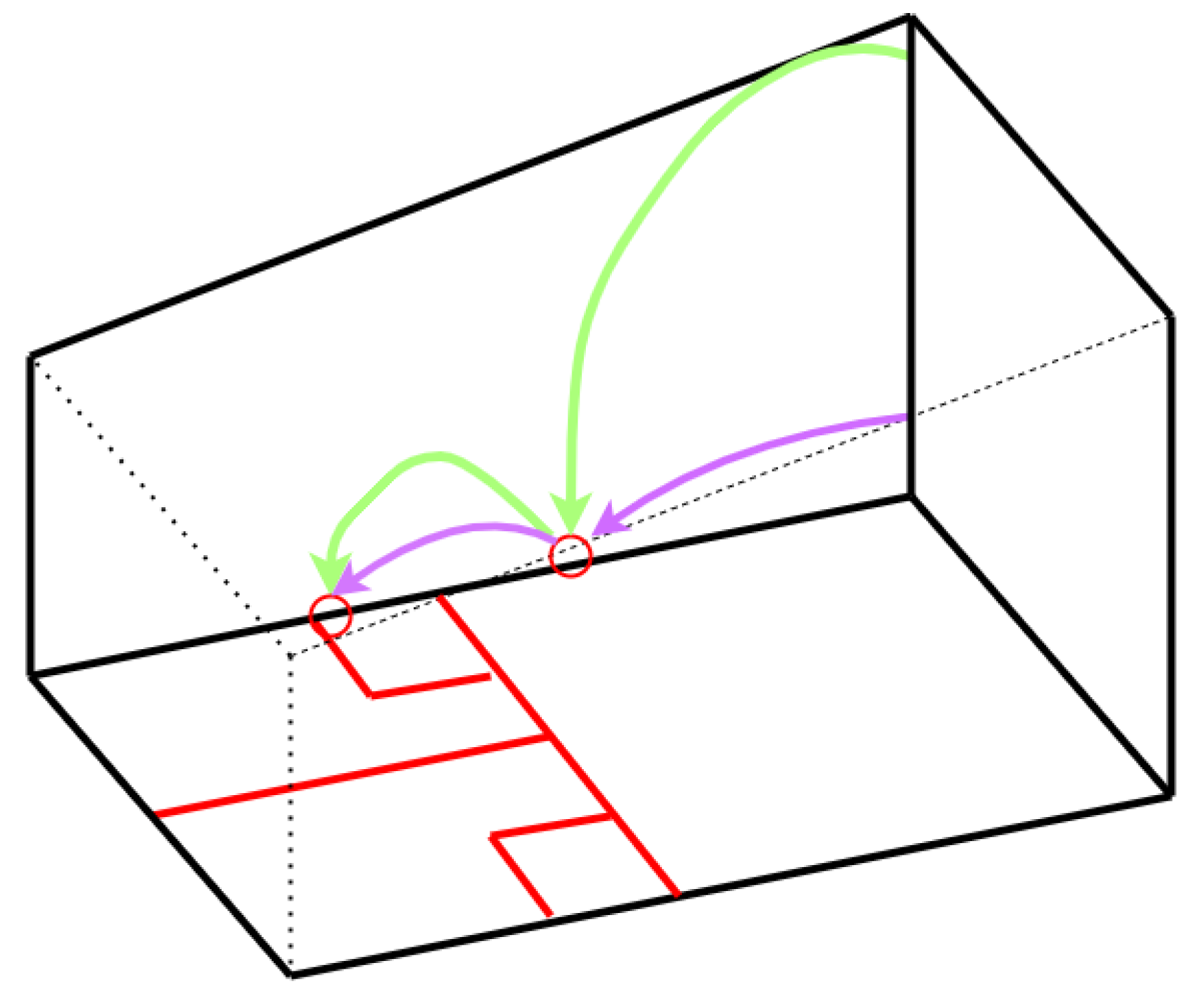
In this case, the AP slipped and fell down. Even though the ball was a little bit far away, the referee deemed this situation a Stroke, because the AP has both blocked the path for too long and provided absolutely no path to the ball by falling down. Had the AP stood still, this situation would probably be considered a Yes Let.
Our model currently does not take clearing time into consideration. To improve on this, more measures should be taken during the data collection process.
5.3.1.8. Speed and Arm Length of Different Players
Naturally, different players have different speeds and reaches. This is also taken into consideration when a referee is making decisions. A player who consistently shows his ability to retrieve hard shots may leave an impression of “fast” to the referee, which potentially makes the referee less inclined to give a No Let to the player.
The speed could be calculated by analyzing video frames or putting motion sensors into the courts. Previous studies have collected data components such as max speed and average speed during squash rallies successfully [15].
5.3.1.9. Situations of No Appeal
Sometimes, when players think they are going to get a No Let decision, they do not appeal at all. From a strategic perspective, appealing and then being rejected disrupts the mentality and flow of one’s game. In our data collection process, we could not take in all of these cases, because although there was interference, there was not any appeal at all.
These situations are hard to classify, as they could also be a mistake from the player; the situation may be given as a Let. In the future, these situations can either be put into the category of No Let, or create the fourth category of “No Appeal" and categorize them as “No Appeal.”
5.3.1.10. Ability to Take Further Movement
The referees evaluate a player’s ability to reach the ball also on the player’s ability to take further movement after the interference.
Figure 41.
Data #249, Ashour/Elshorbagy 2014 World Championship 1:06:12 No Let [35].
Figure 41.
Data #249, Ashour/Elshorbagy 2014 World Championship 1:06:12 No Let [35].
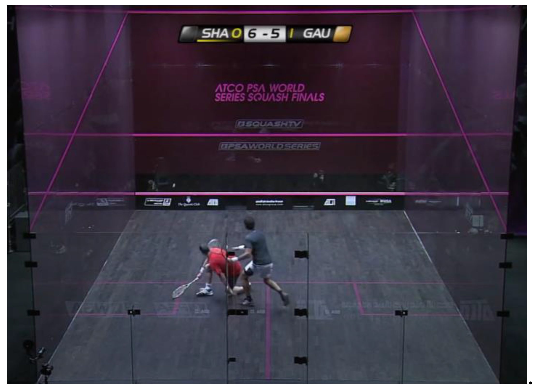
For example, this situation was decided as a No Let. The AP fell down before the contact happened, so he was not able to take further movement from this body position. The referee deemed this situation a No Let because the AP could not have reached the ball, although it was only one step away from him. However, our model does not understand that the AP has fallen down and could not take the extra step to the ball. This is another limitation of this study.
5.3.1.11. Ability to Make Shot
Sometimes, even though the ball is within the reach of the AP, the AP’s ability to make shots can be hindered.
Figure 42.
Not Included in Dataset, Shabana/Matthew 2013 World Tour Finals 59:30 No Let [26].
Figure 42.
Not Included in Dataset, Shabana/Matthew 2013 World Tour Finals 59:30 No Let [26].
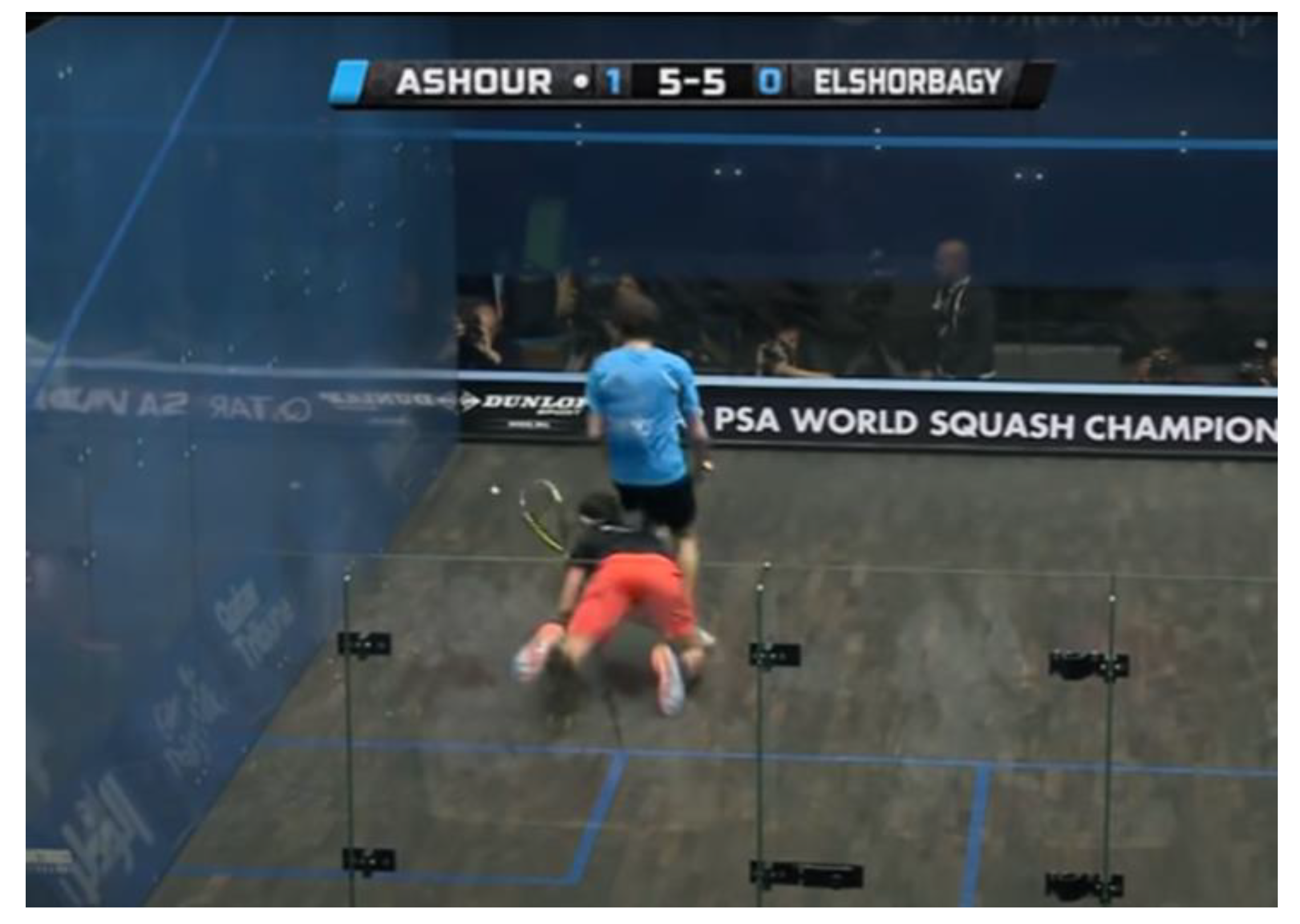
In this case, the ball is right in front of the AP, but the AP could not have hit the ball because it went right into him and his racket could not get in position quickly enough. To our model, this is a case where the ball is close to the AP and the AP is close to the RP, which means it could be a Stroke and is at least a Yes Let. However, in the real-life scenario, the AP is unable to hit the ball, therefore it is decided as a No Let.
5.3.1.12. Degree of Interference
Some interferences can be heavier than others. Usually, the heavier the interference is, the more inclined the referee is to give a Yes Let or a Stroke because it means that the AP’s ability to reach the ball is taken away more.
Figure 43.
Data #157 Matthew/Willstrop 2010 Canary Wharf 39:57 Yes Let [28].
Figure 43.
Data #157 Matthew/Willstrop 2010 Canary Wharf 39:57 Yes Let [28].
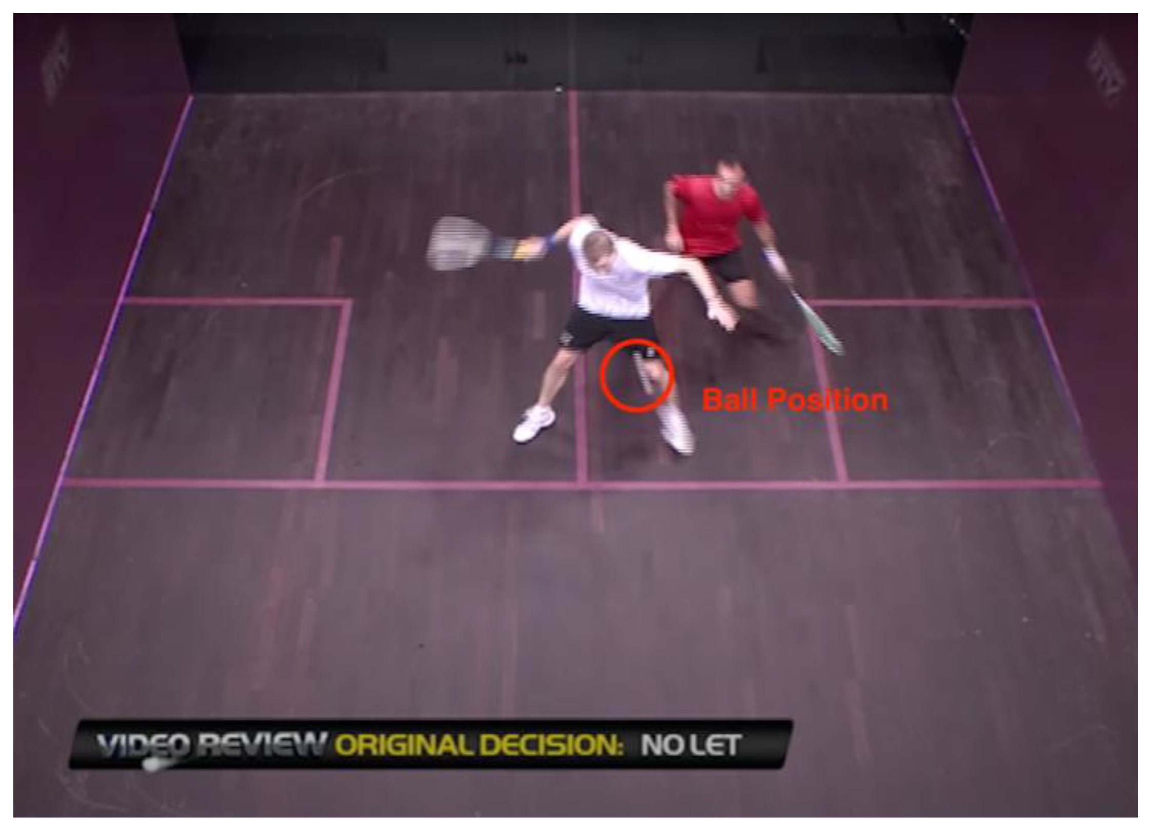
This is an example of one very heavy contact. The AP fell down after tripping on the RP’s foot. Usually, when the AP is taken out completely like this, the referee would not give a No Let no matter how good the ball was.
Our model has no idea of the degree of interference. To account for this, a parameter could be collected by classifying the degree of each interference based on a scale. This is, however, still an objective case and might not be good to be included in the dataset.
5.3.2. Limitations Caused by Abstract Refereeing Concepts
5.3.2.1. Idea of “Wrong Path”
The concept of “wrong path” is an abstract refereeing concept. To retrieve a shot, the AP should take the closest path to the ball. If the AP has taken the “wrong path” and is then blocked by the RP, the referees may give a Yes Let or even No Let.
This case often happens when the AP is first deceived by the shot by RP and goes the wrong way. When the AP realizes and goes to the ball from where he is after the initial movement, he is blocked by the RP. The referees sometimes punish the AP being deceived, in this case, by giving a No Let.
5.3.2.2. Idea of “Accepting Interference”
The concept of “accepting interference” means that the referee deems the AP went through the interference and can play the ball. Thus if the AP then stops and appeals, the referee would give a No Let.
Figure 44.
Data #276, Ashour/Elshorbagy 2014 World Championship 1:21:15 No Let [35]. (a) View taken by the back camera. (b) View taken by the top camera.
Figure 44.
Data #276, Ashour/Elshorbagy 2014 World Championship 1:21:15 No Let [35]. (a) View taken by the back camera. (b) View taken by the top camera.
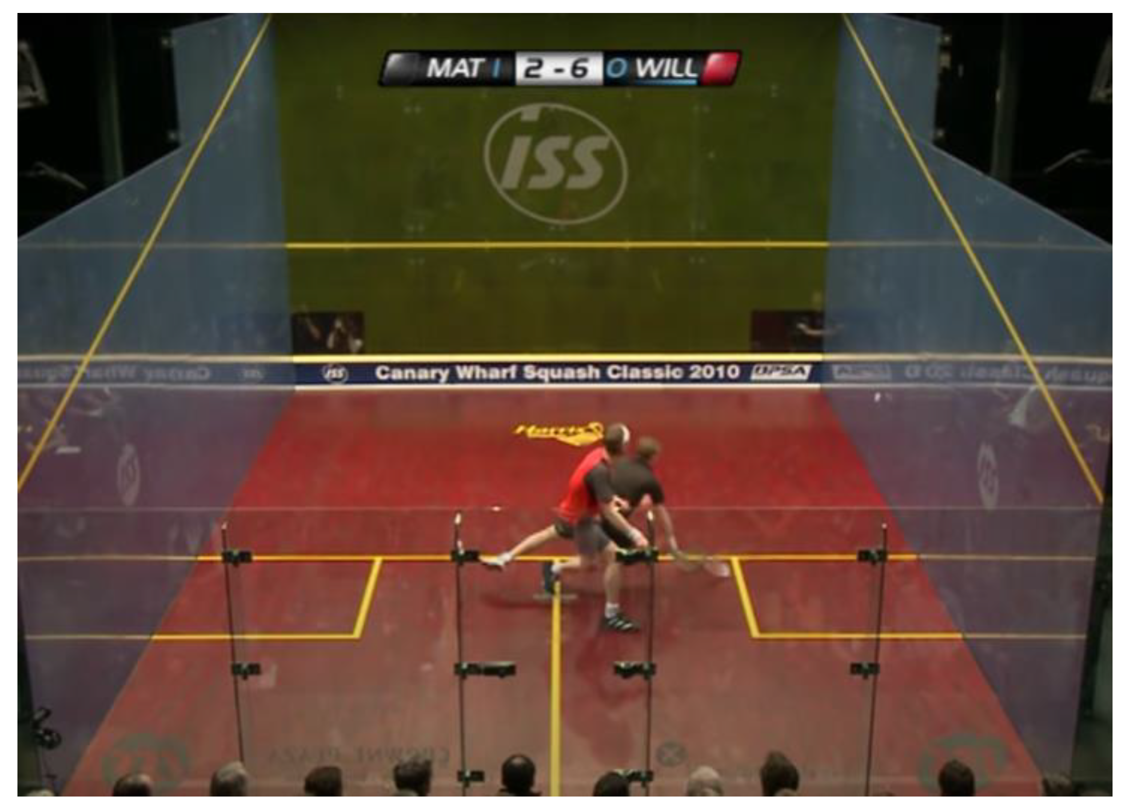
In this case, the AP actually went through the interference and stopped the ball before the second bounce (the AP usually stops the ball to show they can get it, then appeals for a decision). Although the AP showed that he could get it, the referee thought that when he could play the ball, the RP was already away from his swing, and he had “accepted the interference” by going through and reaching the ball. The referee therefore gave a No Let.
This idea of accepting interference varies drastically between different referees. Only referees with harsh standards would impose this concept and give No Lets in this case. Other referees understand that the AP has been impacted on the way to the ball and would give a Yes Let. This remains a controversial idea among referees and audiences.
Our model has no idea what “accepting interference” is. There is no way to learn that although the AP could have reached the ball, he should have played it.
5.3.2.3. Idea of “Minimal Interference” and “Lack of Effort”
When the interference is slight and the AP chooses to not play the ball, some referees give a No Let based on the idea of “minimal interference” and “lack of effort.” The referee wants to promote continuous play, which means that the players need to go through interference that is minimal and show effort that they want to play the ball.
Figure 45.
Not Included in Dataset, Ashour/Gaultier 2013 British Open 41:08 No Let [30].
Figure 45.
Not Included in Dataset, Ashour/Gaultier 2013 British Open 41:08 No Let [30].
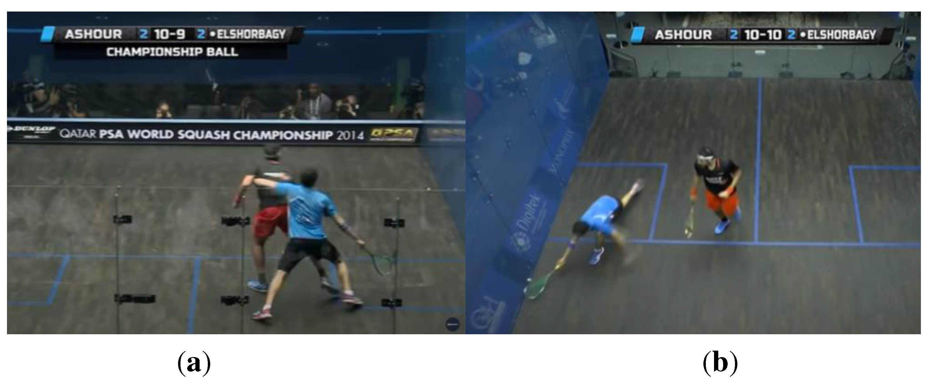
In this case, the AP skimmed through the RP, barely touching him, and decided to stop the ball and appeal. The referee thought that the AP had shown no effort to play the ball, and therefore gave a No Let. The commentators described the situation as this:
“We’ve seen Ramy Ashour (the AP) do this, he does actually get to the ball, but there is interference on his way through… Oh, there’s not much interference, minimal there, it’s minimal. So the question for the referee is why doesn’t he go through and play that? There's not a huge amount of interference. This could stay as a No Let, you know, purely because of lack of effort…He could have clearly played the ball, he elected not to, and he’s paid the price. I think that’s a good decision (No Let).” [54]
Our model would only know that the AP is close to the ball and could have got it. It does not understand that the referee wants to promote continuous play and those situations should be a No Let.
5.3.2.4. Idea of “Punishment for Bad Shot,” “Going Around Opponent,” and “Shut Out”
Figure 46.
Data #43, Matthew/Elshorbagy 2014 British Open 55:56 No Let [25].
Figure 46.
Data #43, Matthew/Elshorbagy 2014 British Open 55:56 No Let [25].
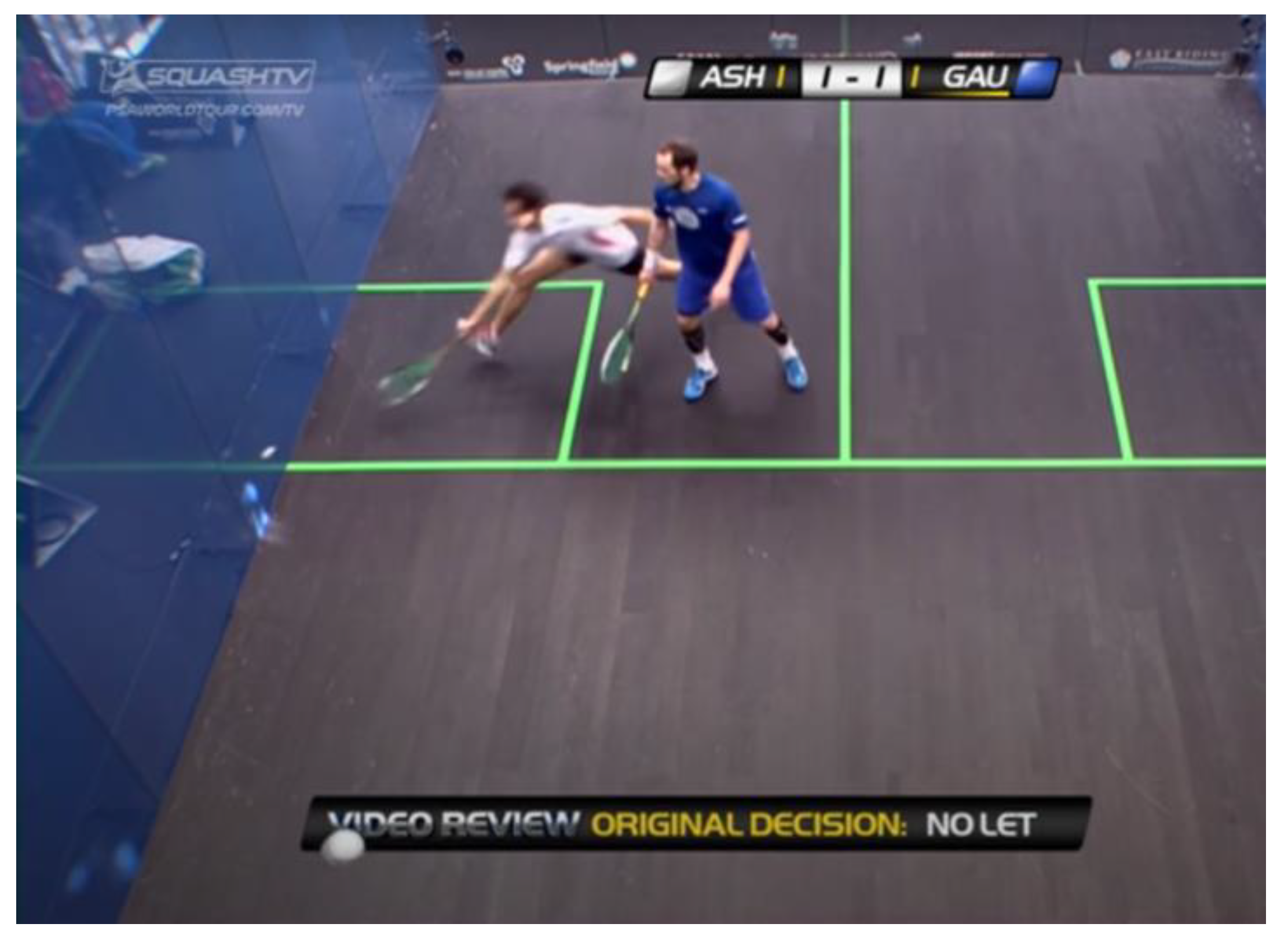
In this case, the AP’s previous shot was loose and the RP hit a ball straight down the left side wall. The AP tried to get it but his path was blocked by the RP. The RP has “shut out” the AP. The referee gave No Let and explained “the ball was too good.” (SQUASHTV, 2014). Here is what the commentators said:
“He’s taken his space there, Elshorbagy (the RP). Loose shot from Nick Matthew (the AP). Nick Matthew has to go around the back of Elshorbagy if he wants to go and get that ball. (The other commentator) Well, it’s his shot to play, Elshorbagy. Definitely his shot to play. But you also, I mean, this is where you get the middle ground. Because it’s his (the RP’s) shot to play, therefore Matthew needs to go around and play the ball, but then he (the RP) also needs to give access” [56].
To the commentators, this could be decided either way: either a No Let, because the AP played a loose ball and therefore should be punished and go the long way through; or a Yes Let, because the RP was not providing the shortest path to the ball.
This is, in fact, a controversial decision as the referees’ ideas collide. The RP is not providing a path (shutting the AP out), but the AP has hit a loose shot and has compromised his position on the court to compensate for the bad shot. Some referees think that in this case, it is justified to punish the AP and give a No Let. Some referees believe that because a path was not provided, it should be given as a Yes Let.
5.3.2.6. Idea of “not allowing to clear”
The idea of “not allowing to clear” describes the situation where the AP holds the RP in position to make the situation look more like a Stroke.
Figure 47.
Data #316, Elshorbagy/Ashour 2014 World Series Finals 37:47 Yes Let [36].
Figure 47.
Data #316, Elshorbagy/Ashour 2014 World Series Finals 37:47 Yes Let [36].
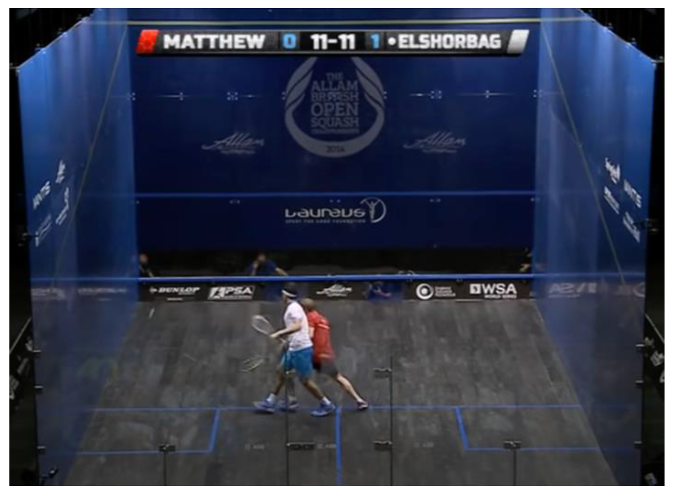
In this case, the AP’s left hand is holding the RP, preventing the RP from exiting the AP’s swing. The referee saw this action and gave a Yes Let instead of a Stroke. If the AP’s left hand was not there, but the RP was in the same position, the referee may have given a Stroke.
5.4. Novel Contributions of this Study
This study is the first study to investigate the process of squash referee decisions and its implications. This study is also the first to propose the use of machine learning as a resolution to refereeing discrepancy in the sport of squash. The proposals of the data collection method and usage of datapoints is unique to this study, along side many detailed analysis of case-specific professional squash decisions. In the process of data collection, the first dataset of refereeing decisions in squash is also made in this study.
6. Conclusions
In this study, we trained neural networks to predict squash referee decisions. Four hundred interferences were collected from public videos as our dataset, and six positional components were annotated, such as the attacking player’s position and the retreating player’s position. Using the six positional components, nine more distance-related components are calculated, such as the distance of the attacking player to the retreating player.
Using combinations of the data components collected, models were trained on Wolfram Mathematica and Python. The results are as follows:
- Wolfram Mathematica achieved a best average accuracy of 86% ± 3.03%; Python achieved a best average accuracy of 85.2% ± 5.1%.
- The accuracies indicate near-human performances, as in most squash matches with 20 to 30 decisions, the referees already make almost three controversial decisions each match.
- Our model has a high potential for improvement, as it is currently being trained with a limited amount of data and a lack of essential information such as the time and the speed. The performance of our model is bound to improve significantly with a larger training data set (say, with 10 or even a 100 times more referee decisions).
- Compared to human referees, the models trained through machine learning follow a singular refereeing standard, do not have a limited attention span, and make decisions almost instantly.
- The model can potentially serve as an extra refereeing official for professional squash matches.
This study makes novel contributions by examining squash referee decision processes and proposing original, innovative solutions to resolve the issue of refereeing discrepancy. This study provides a comprehensive analysis of professional squash decisions while creating the first automated refereeing model for the sport of squash.
7. Future Work
In the future, several measures could be taken to improve the model’s performance.
First of all, simply acquiring more data. This study was trained with only 400 labeled data, which is both limited and unbalanced. If more data were available, the model performance could possibly increase significantly.
Several more methods could be experimented with, such as data augmentation, weighting the data during the training process, and thresholding the output values. The dataset could also be split into two separate sections, one featuring shots where the second bounce is before the service line and another one with shots in which the second bounce is after the service line. This may allow the model to learn more details about how the interferences should be decided.
Some of the new data components could be collected with better tools: speed of the ball, height of the ball, average and max speed of the players, time taken for the ball to die, time taken for the RP to clear, arm length of the player, and the degree of interference. Those values, if considered, could possibly enhance the model’s performance even more.
Supplementary Materials
Although we posted our data on Github, we are happy to submit and share them as Supplementary Materials. We leave this decision up to the Editor and Reviewers.
Author Contributions
Conceptualization, EM and ZJK.; Data curation, Methodology, and Visualization, EM; Project Administration and Formal analysis, EM and ZJK; Supervision, ZJK; Writing – original draft, EM; Writing – review & editing, EM and ZJK.
Funding
This research received no external funding.
Data Availability Statement
Our Dataset is Avaliable at: https://github.com/MaEnqiMark/Dataset_MakingSquashRefereeDecisionsWithMachineLearning.git
Acknowledgements
Thank you to Alan Ji, Benji Kuo, Lucas Yu, and Michael Huang for collecting a separate dataset for exploration purposes, although that part of the study is not included in this final draft. Thank you to Mr Downes, Coach Shabana, Mr Wood, Coach Azam, and my captains, Peter Yuen and Belal Kadry, for instilling in me a love for the sport and inspiring me to play squash competitively.
Conflicts of Interest
The authors declare no conflict of interest.
Appendix A: Remaining four trials for “Training on All Six Data Points”
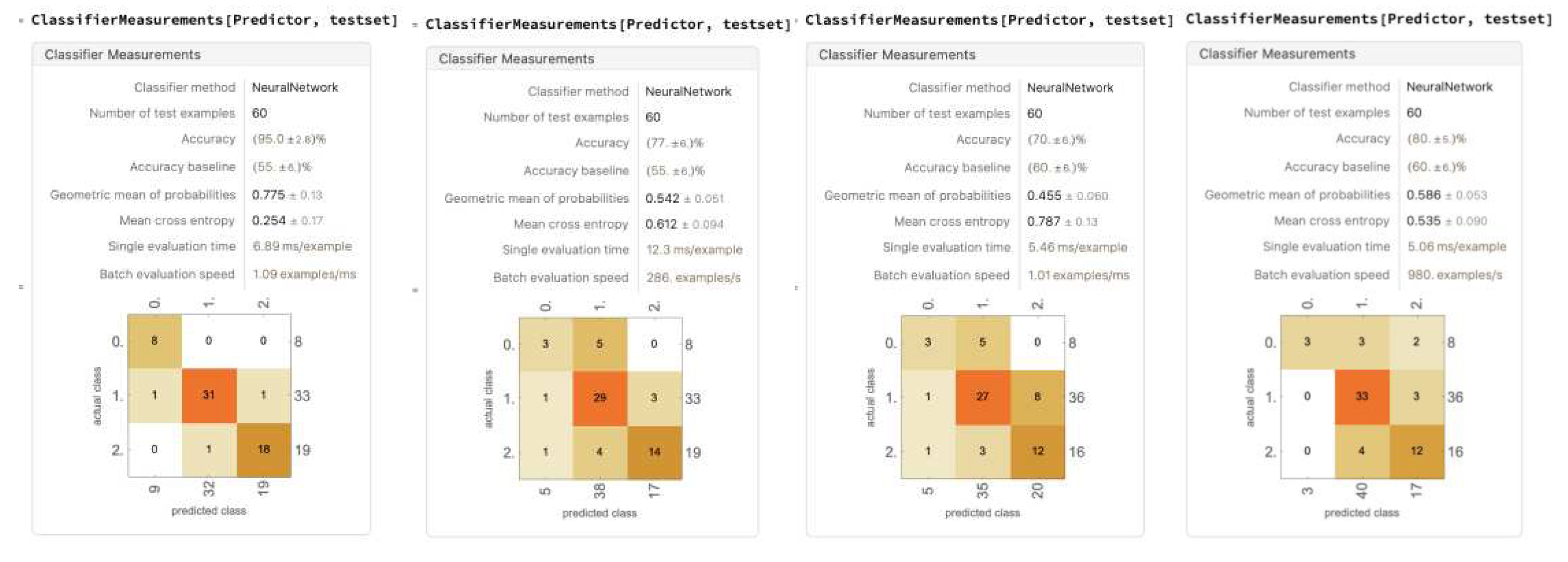
Appendix B: Remaining four trials for “Dropping out Racket Head Position”
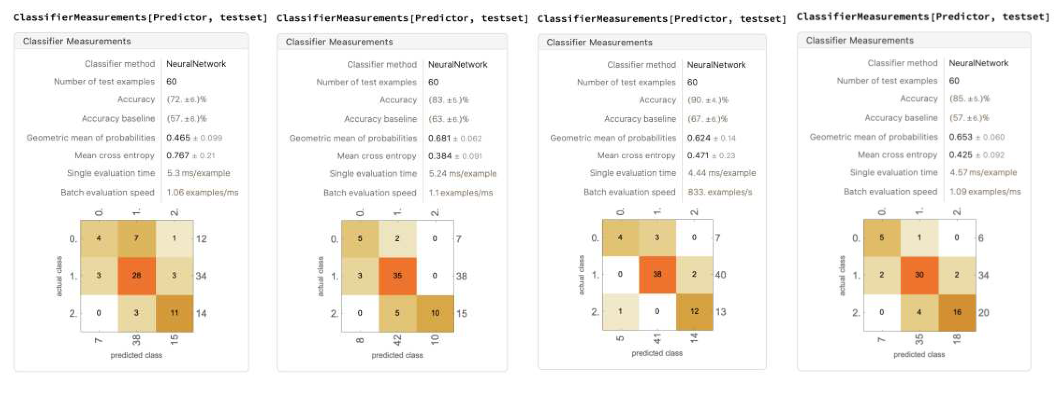
Appendix C: Remaining four trials for “Dropping out Racket Head Position and the First Bounce Position”
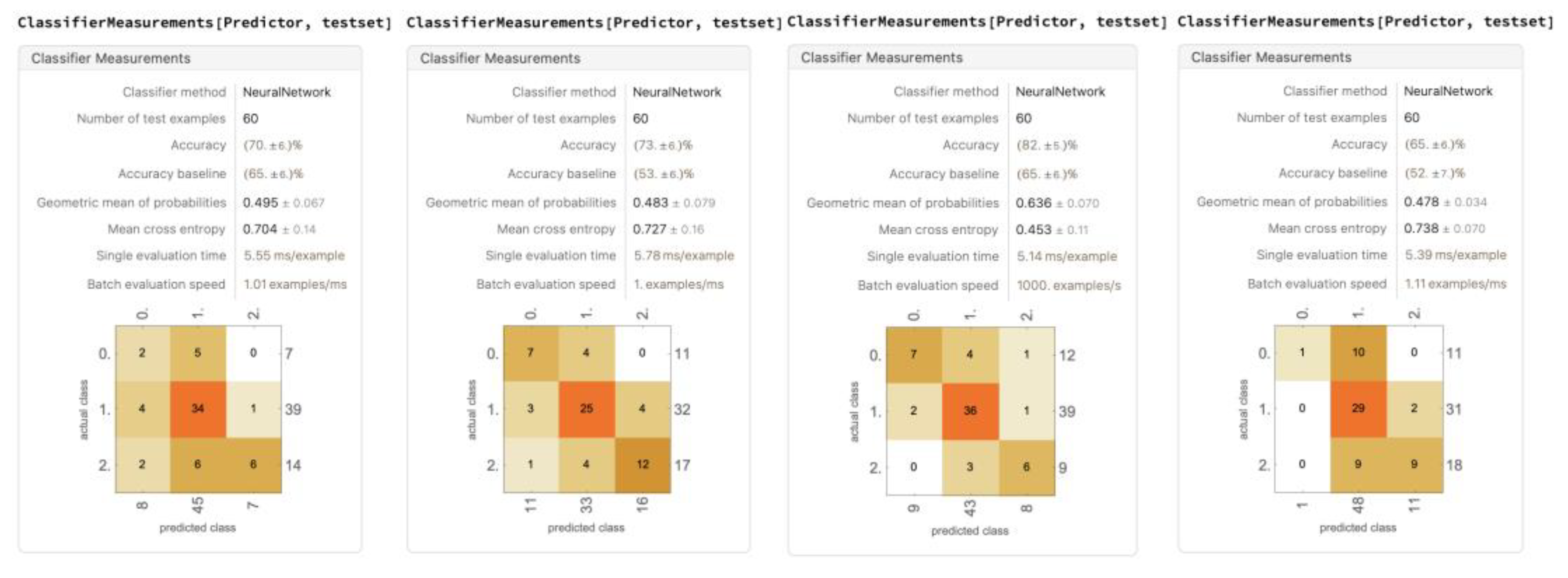
Appendix D: Remaining four trials for “Dropping out Racket Head Position and Second Bounce Position”
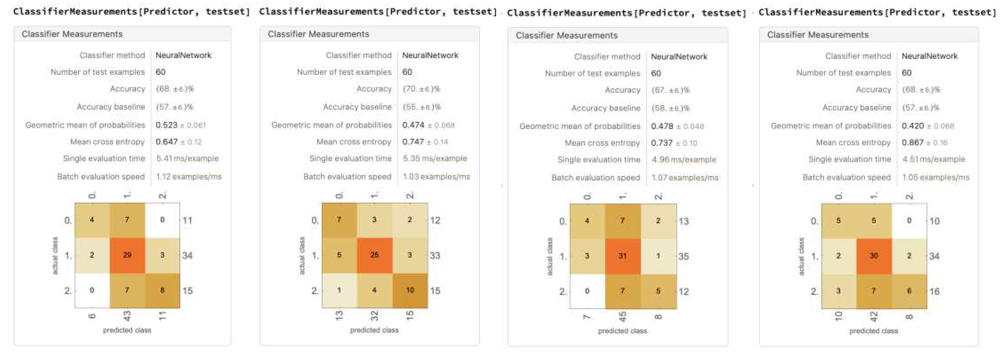
Appendix E: Remaining four trials for “All Nine Modified Data(MD) Points”
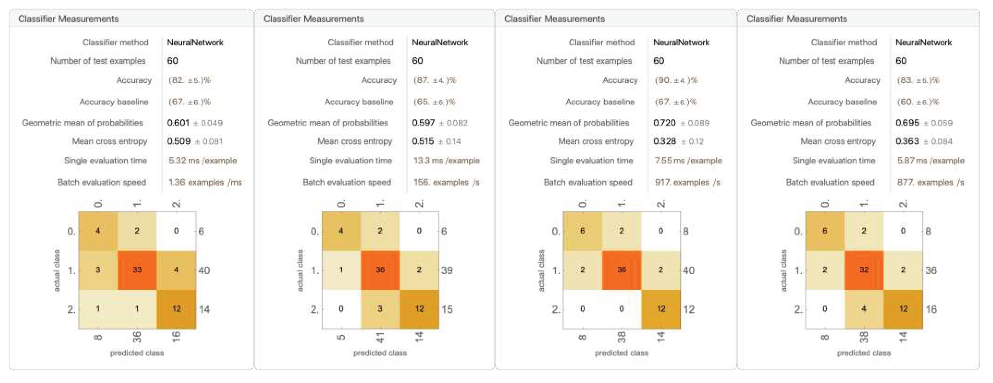
Appendix F: Remaining four trials for “Including MD #1, #2, #3, #4, #6, #8, #9”
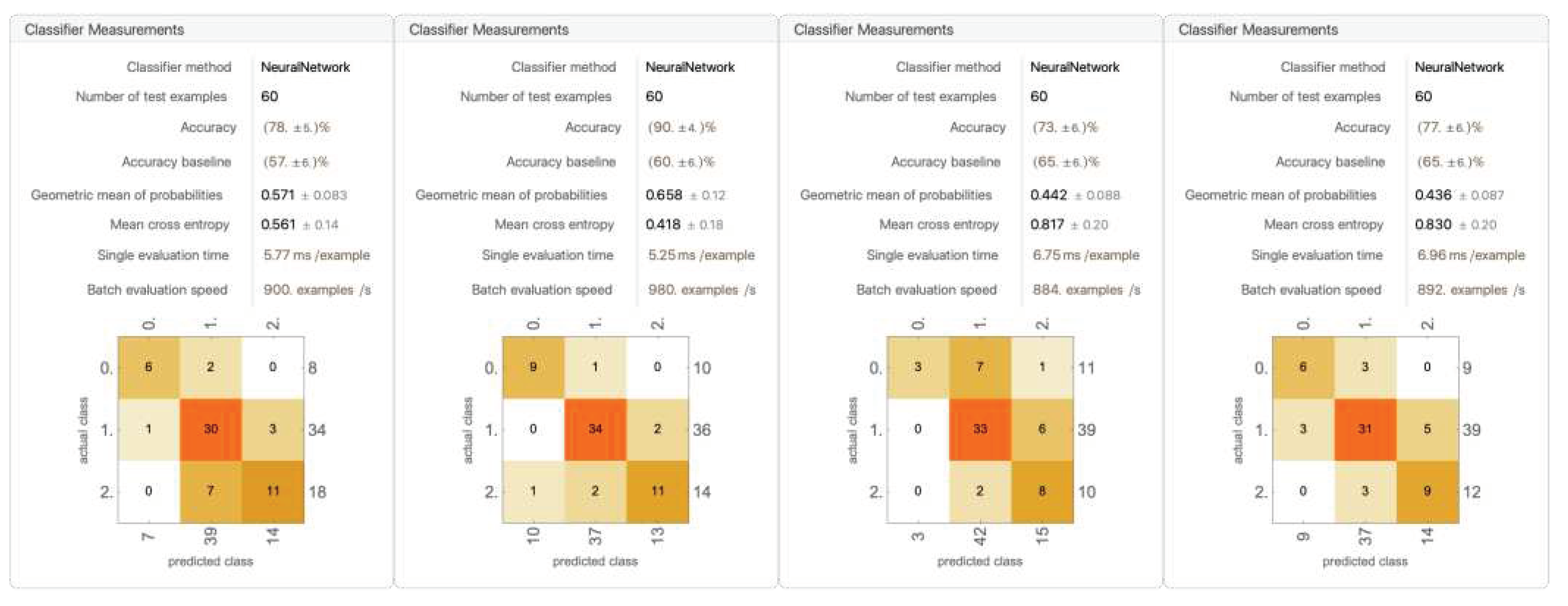
Appendix G: Remaining four trials for “Including MD #1, #2, #3, #4, #6”
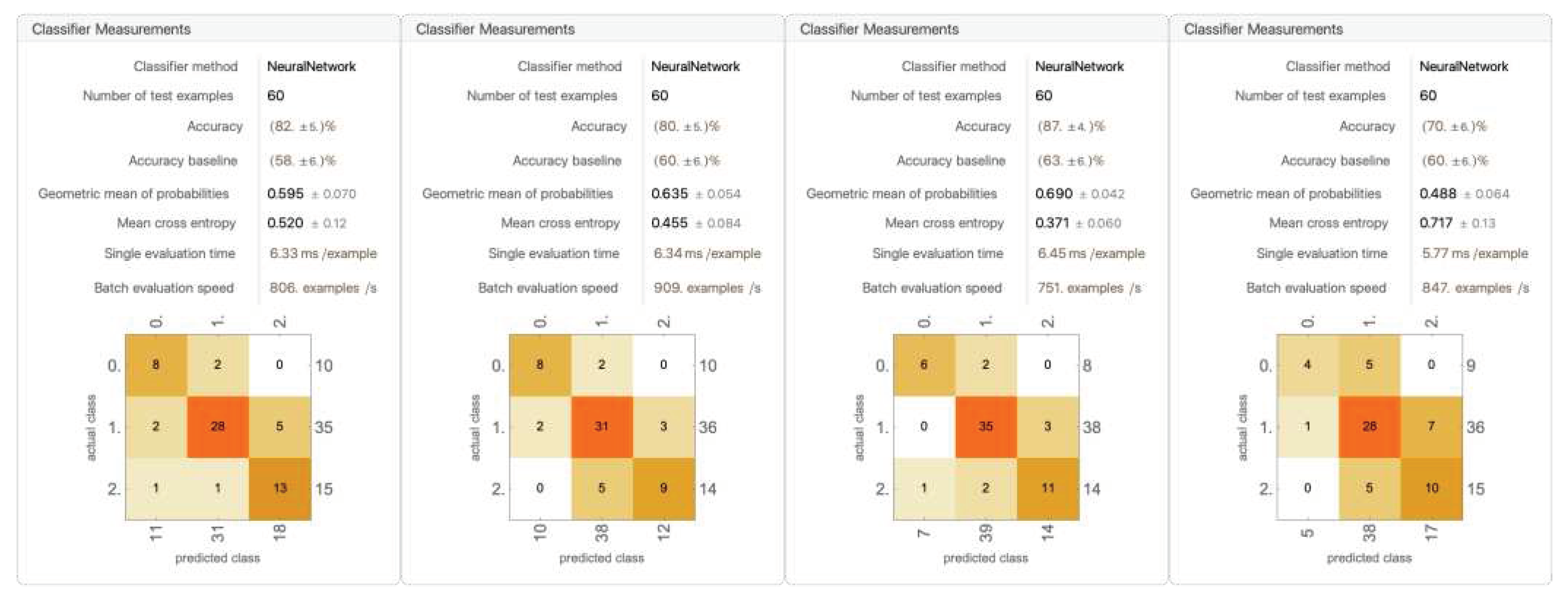
Appendix H: Remaining four trials for “Training with all 21 data points”
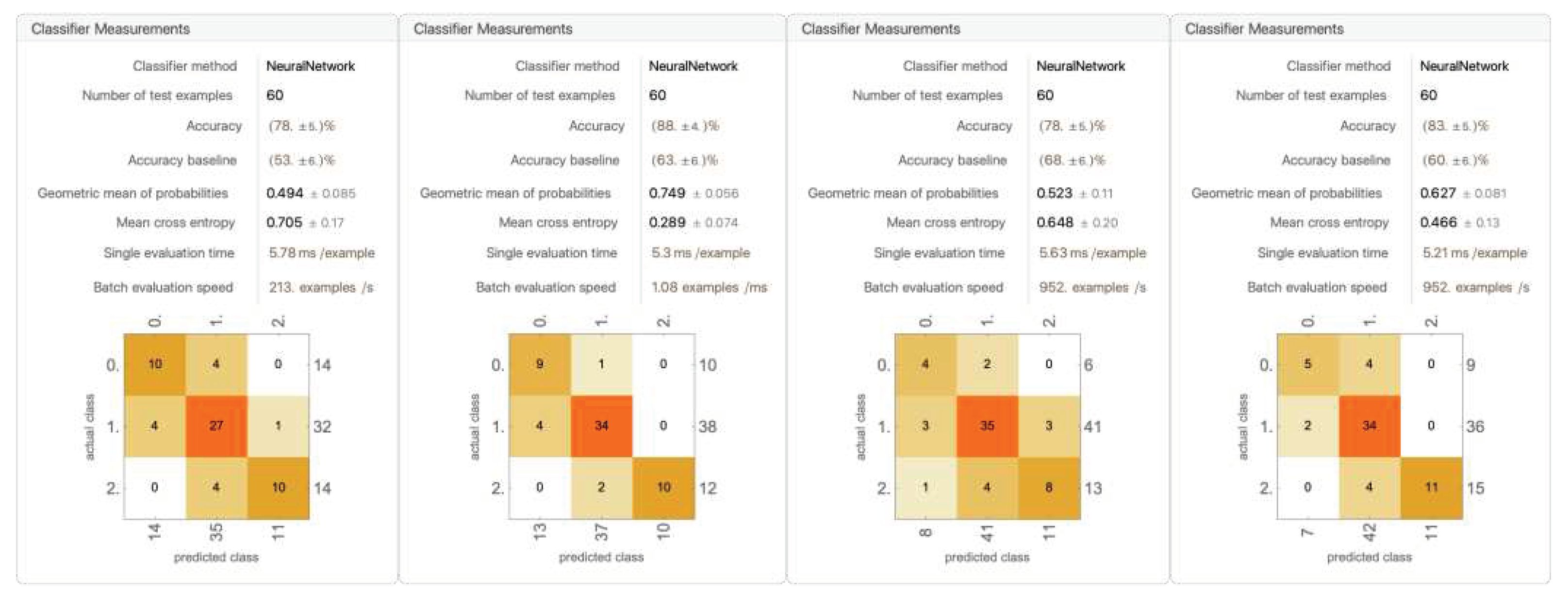
Appendix I: Remaining four trials for “Training with PD 1-10 and all MD”
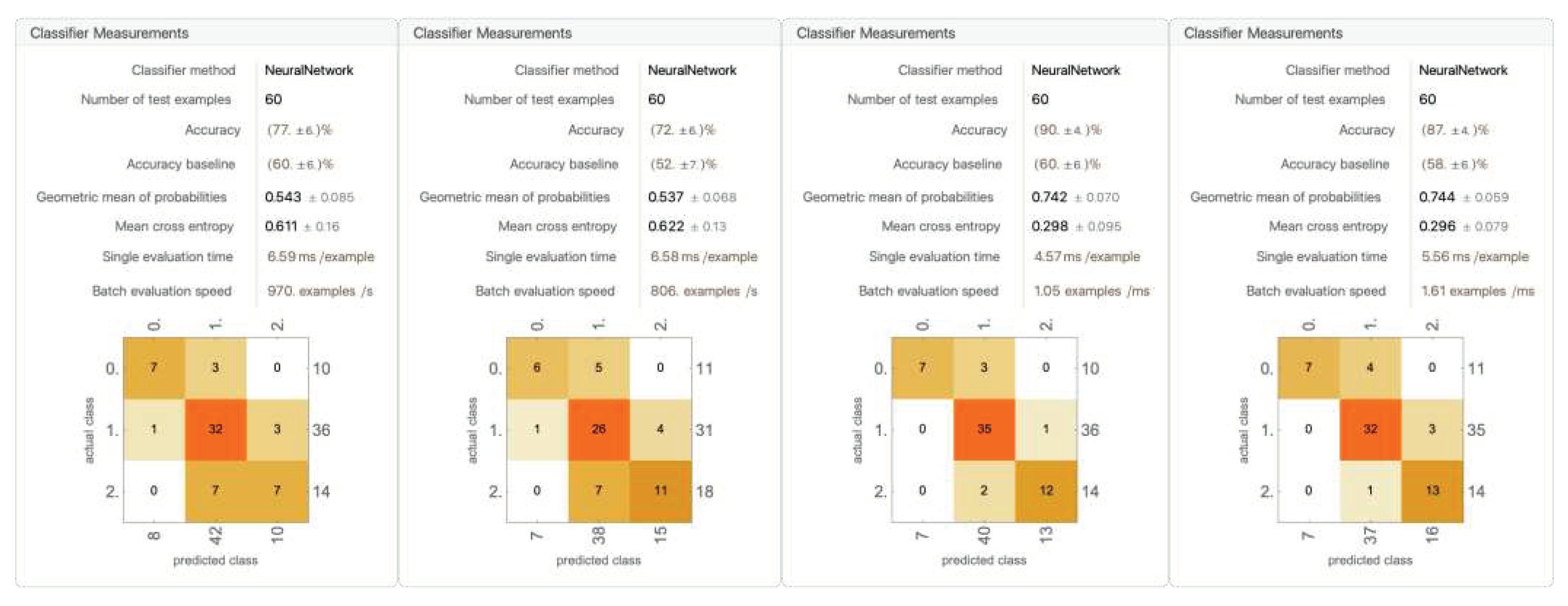
Appendix J: Remaining four trials for “Training with PD 1-10 and MD #3, 5, 6, 8, and 9”
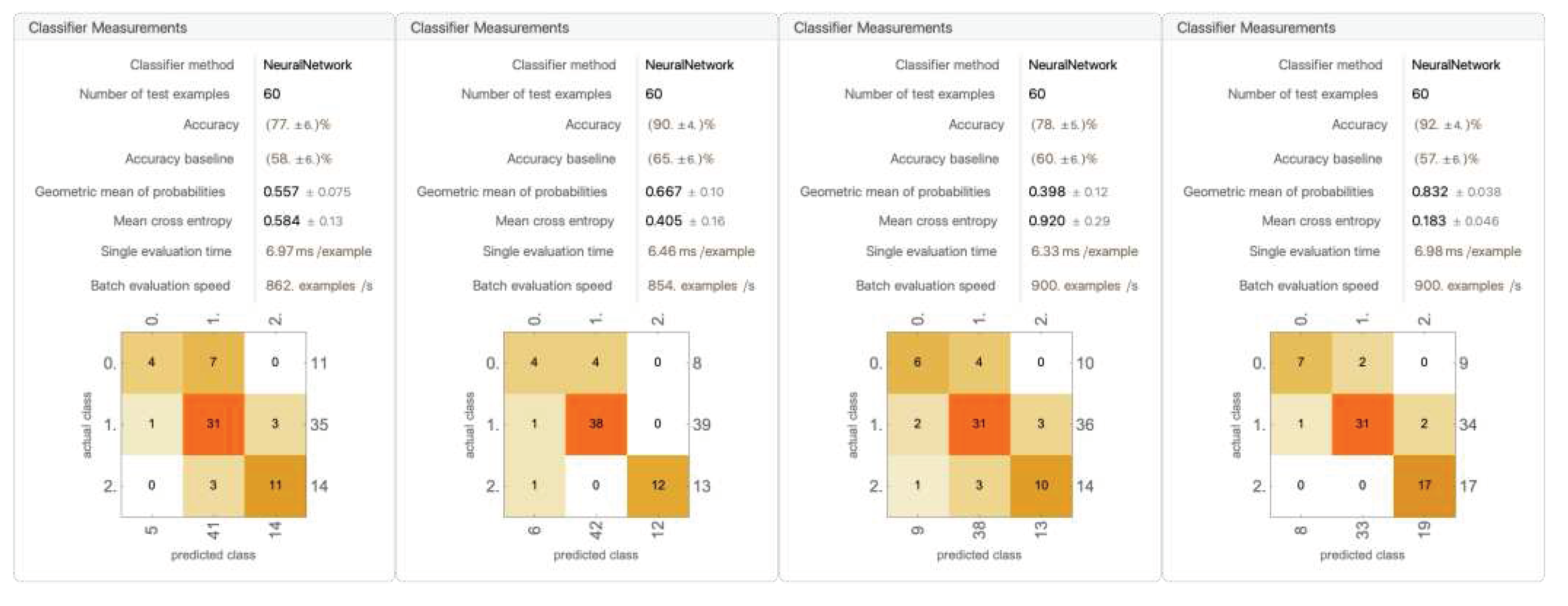
References
- PSA World Tour. (2023, January 26). Squash rules - the basics explained. PSA World Tour. https://www.psaworldtour.com/news/squash-rules-the-basics-explained/.
- SQUASHTV. (2023, June 21). Elias v Asal | World Tour Finals 2022-23 | FREE LIVE MATCH! [Video]. YouTube. https://www.youtube.com/watch?v=Fg_7zxHsFUU&t=2123s.
- Brumann, C., Kukuk, M., & Reinsberger, C. (2021). Evaluation of open-source and pre-trained deep convolutional neural networks suitable for player detection and motion analysis in squash. Sensors, 21(13), 4550. [CrossRef]
- Hu, T., Zheng, M., Li, J. et al. A scene-adaptive motion detection model based on machine learning and data clustering. Multimed Tools Appl 74, 2821–2839 (2015). https://doi-org.ezproxy.oberlin.edu/10.1007/s11042-013-1741-0.
- Menashe, J. et al. (2018). Fast and Precise Black and White Ball Detection for RoboCup Soccer. In: Akiyama, H., Obst, O., Sammut, C., Tonidandel, F. (eds) RoboCup 2017: Robot World Cup XXI. RoboCup 2017. Lecture Notes in Computer Science(), vol 11175. Springer, Cham. https://doi-org.ezproxy.oberlin.edu/10.1007/978-3-030-00308-1_4.
- Hiemann, A., Kautz, T., Zottmann, T., & Hlawitschka, M. (2021). Enhancement of Speed and Accuracy Trade-Off for Sports Ball Detection in Videos—Finding Fast Moving, Small Objects in Real Time. Sensors, 21(9), 3214. MDPI AG. [CrossRef]
- Bayram, F., Garbarino, D., Barla, A. (2021). Predicting Tennis Match Outcomes with Network Analysis and Machine Learning. In: Bureš, T., et al. SOFSEM 2021: Theory and Practice of Computer Science. SOFSEM 2021. Lecture Notes in Computer Science(), vol 12607. Springer, Cham. https://doi-org.ezproxy.oberlin.edu/10.1007/978-3-030-67731-2_37.
- Maier, T., Meister, D., Trösch, S., & Wehrlin, J. P. (2018). Predicting biathlon shooting performance using machine learning. Journal of Sports Sciences, 36(20), 2333-2339. [CrossRef]
- Capobianco, G., Di Giacomo, U., Mercaldo, F., Nardone, V., & Santone, A. (2019). Can Machine Learning Predict Soccer Match Results? In Proceedings of the 11th International Conference on Agents and Artificial Intelligence - Volume 2: ICAART (pp. 458-465). SciTePress. [CrossRef]
- Nguyen, N. H., Nguyen, D. T. A., Ma, B., & Hu, J. (2021). The application of machine learning and deep learning in sport: Predicting NBA players’ performance and popularity. Journal of Information and Telecommunication, 6(2), 217-235. [CrossRef]
- Draschkowitz, L., Draschkowitz, C., Hlavacs, H. (2014). Predicting Shot Success for Table Tennis Using Video Analysis and Machine Learning. In: Reidsma, D., Choi, I., Bargar, R. (eds) Intelligent Technologies for Interactive Entertainment. INTETAIN 2014. Lecture Notes of the Institute for Computer Sciences, Social Informatics and Telecommunications Engineering, vol 136. Springer, Cham. [CrossRef]
- Balmer, Nigel J., Alan M. Nevill, Andrew M. Lane, and Paul Ward. "Influence of crowd noise on soccer refereeing consistency in soccer." Journal of Sport Behavior 30, no. 2 (2007): 130.
- Dohmen, T., & Sauermann, J. (2016). REFEREE BIAS. Journal of Economic Surveys, 30, 679-695. [CrossRef]
- Morgulev, E., Azar, O. H., Lidor, R., Sabag, E., & Bar-Eli, M. (2018). Searching for Judgment Biases Among Elite Basketball Referees. Frontiers in Psychology, 9. [CrossRef]
- Murray, S., James, N., Perš, J., Mandeljc, R., & Vučković, G. (2018). Using a situation awareness approach to determine decision-making behaviour in squash. Journal of Sports Sciences, 36(12), 1415-1422. [CrossRef]
- Professional Squash Association (PSA). (2012, Janurary 9). PSA Squash TV [YouTube Channel]. YouTube. https://www.youtube.com/@squashtv.
- SQUASHTV. (2014, December 25). Squash: Full Match - 2014 El Gouna International SF - Elshorbagy v Gaultier [Video]. YouTube. https://www.youtube.com/watch?v=HyX7IV-YhKo&list=PLxmhcE3iz1lCnuIXg2hOHD29HooENItXg&index=130.
- PSA World Tour. (2011, September 8). PSA to Roll Out Video Review for all TV events. World Squash. https://www.worldsquash.org/psa-to-roll-out-video-review-for-all-tv-events/.
- Chang, YH., Chung, CY. (2020). Classification of Breast Cancer Malignancy Using Machine Learning Mechanisms in TensorFlow and Keras. In: Lin, KP., Magjarevic, R., de Carvalho, P. (eds) Future Trends in Biomedical and Health Informatics and Cybersecurity in Medical Devices. ICBHI 2019. IFMBE Proceedings, vol 74. Springer, Cham. https://doi-org.ezproxy.oberlin.edu/10.1007/978-3-030-30636-6_6.
- Kompella, S., Likith Vishal, B., Sivalaya, G. (2022). A Comparative Study of Classification Algorithms Over Images Using Machine Learning and TensorFlow. In: Shakya, S., Bestak, R., Palanisamy, R., Kamel, K.A. (eds) Mobile Computing and Sustainable Informatics. Lecture Notes on Data Engineering and Communications Technologies, vol 68. Springer, Singapore. https://doi-org.ezproxy.oberlin.edu/10.1007/978-981-16-1866-6_20.
- Gundina, M. A., & Zhdanovich, M. N. (2022). Automatic localization of a car license plate in the Wolfram Mathematica system. SCIENCE and TECHNOLOGY, 21(5), 367-373. [CrossRef]
- Ortigoza, G., & Zapata, U. (2021). Covid-19 Projections: A Simple Machine Learning Approach. In 2021 IEEE International Conference on Engineering Veracruz (ICEV) (pp. 1-4). Boca del Río, Veracruz, Mexico. [CrossRef]
- SQUASHTV. (2020, March 18). PSA Rewind: Willstrop v Gawad - 2018 Grasshopper Cup - Full Squash Match [Video]. YouTube. https://www.youtube.com/watch?v=2T6AXYrhwZQ&list=PLxmhcE3iz1lCnuIXg2hOHD29HooENItXg&index=72.
- SQUASHTV. (2014, December 24). Squash: Full Match - 2014 Tournament of Champions - Shabana v Matthew [Video]. YouTube. https://www.youtube.com/watch?v=OI0xHMRut88&list=PLxmhcE3iz1lCnuIXg2hOHD29HooENItXg&index=125.
- SQUASHTV. (2014, December 25). Squash: Full Match - 2014 British Open SF - Matthew v Elshorbagy (British Open) [Video]. YouTube. https://www.youtube.com/watch?v=nwzMnIECgDk&list=PLxmhcE3iz1lCnuIXg2hOHD29HooENItXg&index=127.
- SQUASHTV. (2019, June 5). Squash Archive: Shabana v Matthew - 2012/13 World Tour Finals [Video]. YouTube. https://www.youtube.com/watch?v=AASrbKRyAUo&list=PLxmhcE3iz1lCnuIXg2hOHD29HooENItXg&index=79.
- SQUASHTV. (2013, December 24). SQUASH: Full Match - 2012 PSA World Championship Final - Ashour v Elshorbagy [Video]. YouTube. https://www.youtube.com/watch?v=s6QcWY5wEak&list=PLxmhcE3iz1lCnuIXg2hOHD29HooENItXg&index=119.
- SQUASHTV. (2013, October 5). Squash: Full Match - Canary Wharf 2010 SF - Matthew v Willstrop [Video]. YouTube. https://www.youtube.com/watch?v=HtwckCfSIHU&list=PLxmhcE3iz1lCnuIXg2hOHD29HooENItXg&index=118.
- SQUASHTV. (2013, October 5). Squash: Full Match - 2011 World Series Finals, Final - Shabana v Gaultier [Video]. YouTube. https://www.youtube.com/watch?v=fdYZePDe69s&list=PLxmhcE3iz1lCnuIXg2hOHD29HooENItXg&index=118.
- SQUASHTV. (2016, March 18). Squash: Free (Match) Friday - Ashour v Gaultier - British Open 2013 Final [Video]. YouTube. https://www.youtube.com/watch?v=5O3fpxcExu0&list=PLxmhcE3iz1lCnuIXg2hOHD29HooENItXg&index=115.
- SQUASHTV. (2019, December 25). Squash: Farag v Coll - Full Match - British Open 2019 - Christmas Cracker [Video]. YouTube. https://www.youtube.com/watch?v=ntNh7L1pTag&list=PLxmhcE3iz1lCnuIXg2hOHD29HooENItXg&index=77.
- Saini, V. (2023, April 18). Average shoulder width for men and women. Fitness Volt. https://fitnessvolt.com/average-shoulder-width/#:~:text=According%20to%20the%20same%20CDC,the%2030%2D39%20age%20group.
- Wolfram. (n.d.). Classifying Data with Neural Networks. Classifying data with neural networks-wolfram language documentation. https://reference.wolfram.com/language/tutorial/NeuralNetworksClassification.html.
- SQUASHTV. (2018, December 18). Squash: 100k Subscriber Special - Matthew v Gaultier ToC 2018 Full Match [Video]. YouTube. https://www.youtube.com/watch?v=6lniVi_ScJI&list=PLxmhcE3iz1lCnuIXg2hOHD29HooENItXg&index=82.
- SQUASHTV. (2014, December 25). BEST SQUASH MATCH EVER? 2014 World Championship Final: Ashour v Elshorbagy - Full Match [Video]. YouTube. https://www.youtube.com/watch?v=-xs8EUlCL5o&list=PLxmhcE3iz1lCnuIXg2hOHD29HooENItXg&index=116.
- SQUASHTV. (2016, May 6). Squash: Free (Match) Friday - 2013/14 World Series Finals - Elshorbagy v Ashour FINAL [Video]. YouTube. https://www.youtube.com/watch?v=lpEQp1raU00&list=PLxmhcE3iz1lCnuIXg2hOHD29HooENItXg&index=113.
- SQUASHTV. (2012, June 22). Squash: Full Match - 2012 British Open SF - Willstrop v Ashour [Video]. YouTube. https://www.youtube.com/watch?v=8eaAa0R4nck&list=PLxmhcE3iz1lCnuIXg2hOHD29HooENItXg&index=120.
- SQUASHTV. (2019, April 23). Squash: Ramy Retirement Special - Full Match - Ashour v ElShorbagy - Grasshopper Cup 2018 [Video]. YouTube. https://www.youtube.com/watch?v=yhKcp2QpdI4&list=PLxmhcE3iz1lCnuIXg2hOHD29HooENItXg&index=80.
Disclaimer/Publisher’s Note: The statements, opinions and data contained in all publications are solely those of the individual author(s) and contributor(s) and not of MDPI and/or the editor(s). MDPI and/or the editor(s) disclaim responsibility for any injury to people or property resulting from any ideas, methods, instructions or products referred to in the content. |
© 2023 by the authors. Licensee MDPI, Basel, Switzerland. This article is an open access article distributed under the terms and conditions of the Creative Commons Attribution (CC BY) license (http://creativecommons.org/licenses/by/4.0/).
Copyright: This open access article is published under a Creative Commons CC BY 4.0 license, which permit the free download, distribution, and reuse, provided that the author and preprint are cited in any reuse.


