
Submitted:
29 November 2023
Posted:
30 November 2023
You are already at the latest version
Abstract
In order to achieve the target, several activities are being undertaken, including the development of multipurpose reservoir planning for the water supply and sanitation infrastructure, irrigation, and hydropower development for the H project. To undertake this work, the main data given was rainfall data, flow data, catchment area, base population for water supply, and so on. This report presents a specifically preliminary study and design of water supply, irrigation, and hydropower development for the project, which is carried out in accordance with the scope of work given by our professor. The preliminary study and design are therefore to investigate scenarios and alternatives and prepare a document of water supply, irrigation, and hydropower infrastructures for the provision of the assignment. This report, as required in the assignment, contains project background, water sources assessment, selection of suitable hydropower potential, and irrigation sizing, design criteria, descriptions of the proposed scheme, preliminary design of water supply components. The objective of the project is to recommend and design a cost-effective water supply system, irrigation, and hydropower development to supply reliable, sufficient, and safe water from a defined water source to the H project. The specific objectives of the investigation works are: • To assess potential water source alternatives for water supply • Selecting appropriate size for the reservoir which could satisfy all water demand • Assess and select suitable irrigation development and hydropower potential. • Preliminary study and design of all components of the reservoir and appurtenant structures The scope of the project generally focuses on preliminary study and design of water supply, irrigation and hydropower development components from water sources potential and the water balance output.
Keywords:
Hydropower
; Irrigation
; water supply
; pre-feasibility
1. Introduction
1.1. General
The main purpose of this project is to enable us work and make exercise on multipurpose reservoir planning. And, this project is undertaken and worked according to the specific guidelines and science of water science and engineering in the study and design of a multipurpose reservoirs.
1.2. Project background
In order to achieve the target several activities are undergoing with the development of multipurpose reservoir planning of the water supply and sanitation infrastructure, irrigation and hydropower development for H project. To undertake this, work the main data given was rainfall data, flow data, catchment area, base population for water supply and so on.
This report presents specifically preliminary study and design of water supply, irrigation and hydropower development for the project, which is carried out in accordance with the scope of works given by our professor. The preliminary study and design is therefore to investigate scenarios, alternatives, and prepare the document of water supply, irrigation and hydropower infrastructures for the provision of the assignment.
This report, as required in the assignment, contains: project background, water sources assessment, selection of suitable hydropower potential, and irrigation sizing, design criteria, descriptions of the proposed scheme, preliminary design of water supply components.
1.3. Project objective
The objective of the project is to recommend and design cost effective water supply system, irrigation and hydropower development; to supply reliable, sufficient and safe water from defined water source to the H project. Specific objectives of the investigation works are;
- To assess potential water source alternatives for water supply
- Selecting appropriate size for the reservoir which could satisfy all water demand
- Assess and select suitable irrigation development and hydropower potential.
- Preliminary study and design of all components of the reservoir and appurtenant structures
1.4. The scope of the project
The scope of the project generally focuses on preliminary study and design of water supply, irrigation and hydropower development components from water sources potential and the water balance output.
1.5. Limitations of the study
There are some data limitations encountered during the study and preliminary studies including;
- Longest path, rigidity/slope of the catchment
- Lack of topographic data as with required scale and accuracy.
2. Approaches and materials used in the study
2.1. Materials Used
The following materials were used during the study, these are spreadsheet models are developed for all works as follows
- Filling missing data
- Flood frequency analyses
- Catchment yield calculation
- Flood routing
- Water balance and demand analyses
- Estimation of hydropower potential and irrigation sizing
2.2. Approaches used
2.2.1. Field Work
Since this assignment is worked out from the given data so, no any fieldwork is undertaken.
2.2.2. Office/ Desk Work
In the office/desk work different activities have been carried on including;
- Identification of secondary data requirement of the project area.
- Collection of relevant secondary data
- Review of previous studies conducted, relevant documents pertaining to the assignment.
- Identify potential water sources for water supply, irrigation & hydropower
- Summarizing, analysis, interpretation of collected data, Conduct preliminary design of water supply, irrigation & hydropower.
2.2.3. Results of Field and Desk work
After performing intensive office work, outputs and result of the different aspects of water supply system: reservoirs options, hydropower potential, and spillway appurtenant structures are identified and presented below. The design will be based on the Federal Ministry of Water Resource Design guideline, different design reports, text books and field work conducted in similar projects to collect important data for the design work.
2.2.4. Stakeholder consultation
Stakeholders like for such mega projects are critical in making stakeholder consultation. The aim was to get ideas and views, how they understood the proposed project and consider their feedback and say towards successful selection, design and implementation of the project. Presentation of the preliminary phase of study with client representatives in project office will be significant to consider additional water source options.
3. Project Description
3.1. Location
The project H is a multipurpose reservoir for water supply, hydropower and irrigation development located in X and Y Coordinate.
3.2. Accessibility
The accessibility of the project is unknown.
3.3. Climate
Before undertaking any analyses of climate data homogeneity, consistency and normality test of climate data are mandatory[1]. The climatic condition of the project area has warm climatic condition. The project areas mean rainfall series estimated from 50 years’ (1951-2000) record of stations. These estimations revealed that the annual average rainfall over the project is estimated to be 1284 mm.
3.4. Estimation of stream flow missing data
The main purposes of this part of study are to evaluate missing stream flow data using several interpolation methods which are arithmetic average (AA) method, normal ratio (NR) method, inversed distance (ID) method, and coefficient of correlation (CC) method[2]. However, if the data are still missing and information from surrounding stations cannot be utilized due to a lack of data, the mean for the same day and month but in a different year is used to estimate the missing values on that specific day. To assess missing values at the target station using information from surrounding stations, the analysis would be separated into four or more distinct percentages, such as 5%, 10%, 15%, and 20%, to reflect various types of missing data [2]. However, just 20% (10 years' worth of missing data from 50 years) is considered for this experiment. Additionally, the Mean Absolute Error (MAE), Correlation Coefficient (R), and Root Mean Square Error (RMSE) tests are used to compare the effectiveness of various strategies [2].
3.4.1. Estimation Methodology
There are two primary subsections in this section. We'll talk about missing data estimation techniques in the first subsection. The target and a few carefully chosen nearby stations were included in the analysis. In the meanwhile, the second part will cover evaluating the effectiveness of the employed techniques. The target station contains all of the data in the first part. Next, data at the target station are taken to be missing in order to evaluate the estimating techniques. The target station's missing stream flow and rainfall data are compared to the actual records using interpolation techniques.
3.4.2. Interpolation methods
(i) Arithmetic Average Method
The arithmetic average (AA) Two major subsections comprises this section. The first topic will provide techniques for estimating missing data. A study was conducted with a target and a few carefully chosen nearby stations. The second subsection will include evaluating the effectiveness of the employed techniques in the interim. The target station possesses the entire collection of data in the first segment. Afterwards, data at the target station are taken to be missing in order to evaluate the estimating techniques [3, 4].. The missing stream flow and rainfall data at the target station are compared to the real records using interpolation techniques.
Where xi is the observed data at ith neighboring stations or the date of the same date with various years, n is the number of nearby stations or number of years, and pt is the predicted value of the missing data at the t target station/date.
(ii) Normal Ratio Method
The target station's and its surrounding station's ratio mean of accessible data is the basis for the weighting of the normal ratio (NR) approach. This approach is applied if any nearby stations have data on typical annual rainfall and stream flow that surpasses ten percent of the station under consideration [5, 6].. Given by is the estimated missing value.
Where Nt is the annual rainfall and stream flow amount at the target station and Ni is the annual rainfall and stream flow amount at the ith nearby station.
(iii) Inverse Distance Method
The approach that is most frequently used to estimate missing data is the inverse distance (ID) method. The target station's distance from the neighboring station is the basis for this strategy. Compared to further stations, the nearby stations have a stronger correlation with the target station[5, 6]. Given by is the estimated missing value.
where dit is the distance between target station and the ith nearby station.
(iv) Coefficient of Correlation Method
correlation coefficient (CC) Using this strategy, the correlation coefficient is employed as the weighting value instead of the distance [7]. Given by is the estimated missing value [8].
where rit is the correlation coefficient of daily time series data between the target station and the ith nearby station.
3.4.3. Performance of the estimation methods
Three performance criteria are applied in this study [9]. To assess spatial interpolation techniques, statistics such as the correlation coefficient (R), mean absolute errors (MAE), and root mean square errors (RMSE) are computed. The difference between the estimation values and the matching observed values is measured by the error. Better results will be shown by RMSE and MAE, which show lower values. Meanwhile, correlation coefficient indicates the strength of the relationship between observations and estimates which the higher positive coefficients estimate the best results.
where xi is the observed rainfall and stream flow at nearby station, xiˆ is the estimated value and is the number of nearby station.
3.4.4. Results and discussion of estimation methods
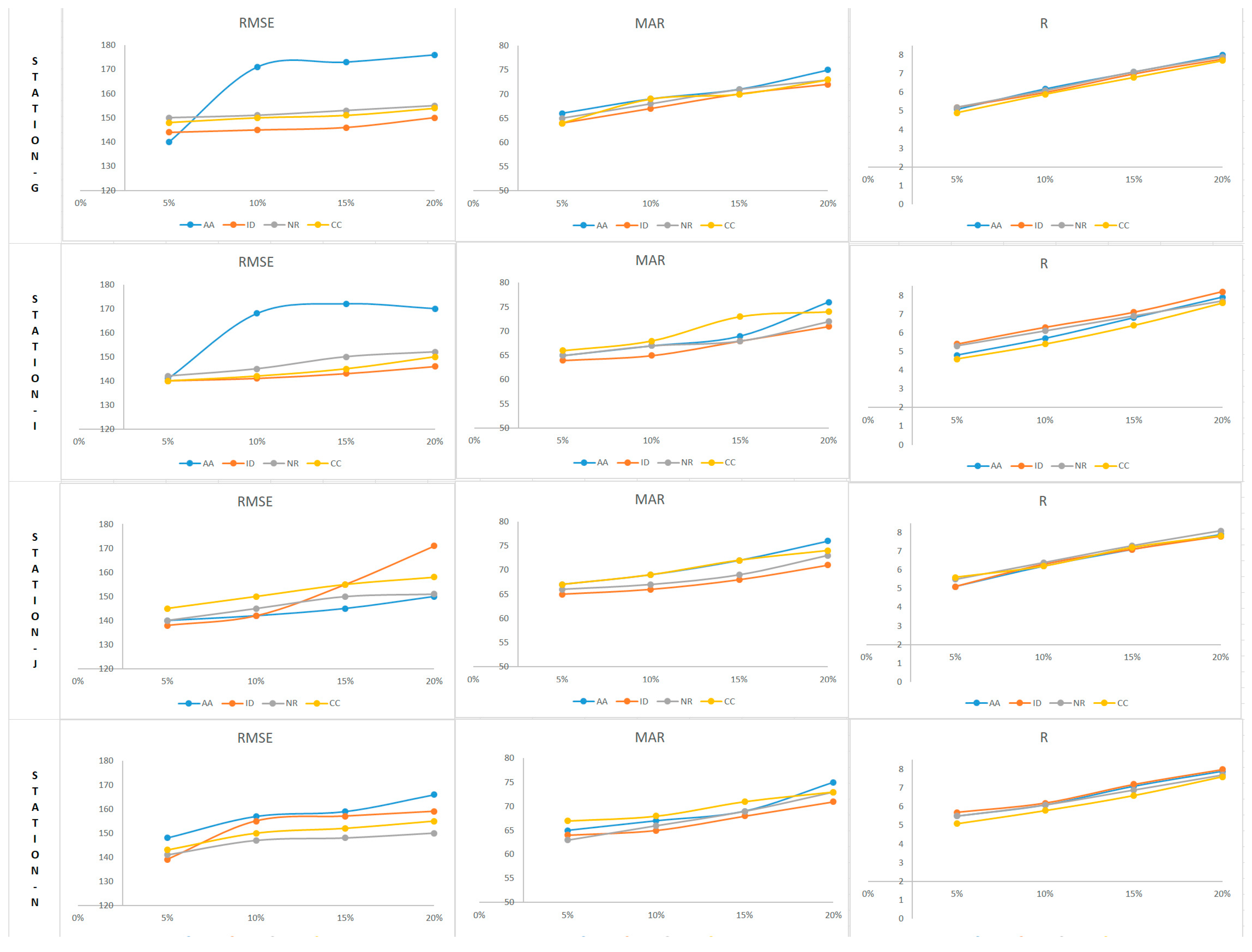
We shall touch on the analysis's findings in this part. We tried each of the four interpolation techniques on a single percentage at 20 percent. The table below, Table 3-1, presents the findings of the approaches' overall performance. The comparison of flow data estimating techniques is presented in Table 3-1. For G, I, and J stations, the ID approach is proven to be the most effective. NR is the most effective approach for N station. Additionally, it is demonstrated that for all stations that produced the lowest RMSE, the CC technique is the second-best approach. Additionally, Table 3-2 just compares the estimating techniques with four distinct percentages of missing values—that is, five, ten, fifteen, and twenty percent.
Figure 3-1.
Comparison of RMSE, MAE and R method with various percentages of missing values for G. I, J and N Stations.
Figure 3-1.
Comparison of RMSE, MAE and R method with various percentages of missing values for G. I, J and N Stations.
4. Water Demand, Sources and Storage
4.1. Water Demand of the Project
The design basis for the sizing of any water resource planning is first of all an estimate of the amount of water expected to be used by the project [10]. Accurate estimate of water demand is a basic consideration to the sizing of storage facilities, this involves consideration of a number of factors depending on the nature of the project [11].
The water demand required for the development of water supply, irrigation and hydropower has been fixed and estimated by the following procedures.
Based on client provision the project water supply demand is estimated to be 100lit/day/cap and crop water and irrigation requirement is given below in Table 4-1 and for the hydropower it is to be decided at later stage after analyses.
4.2. Surface Water Sources
The project must have water source with sufficient capacity and reliably to full fill the water demand.
4.2.1. General site selection criteria for the reservoir
- The reservoir site should be such that the leakage of water through the ground is minimum
- Sites having permeable rocks reduce the water tightness of the reservoir. The rocks which allow less passage of water include shales, slates, schists, gneiss, and crystalline igneous rocks such as granite.
- A suitable site for the darn must exist. The dam should be founded on sound watertight rock base, and percolation below the dam should be minimum. The cost of the dam depends on the suitability of a site and is often a controlling factor in the site selection.
- The reservoir basin should have a narrow opening in the valley so that the length of the dam is the least possible.
- The cost of the real estate for the reservoir, including road, railway, rehabilitation and resettlement etc. must be as small as possible.
- The topography of the reservoir site should be such that, it has adequate storage capacity without submerging excessive land and other properties.
- The site should be such that a deep reservoir is formed. A deep reservoir is preferable to a shallow one because of the lower cost of the land submerged per unit of capacity, less evaporation losses due to reduction in the water spread area, and less likelihood of weed growth.
- The reservoir site should be such that it avoids or excludes water from those tributaries which have a high concentration of sediments in water.
4.3. Elevation-Area-Capacity Curves
According the given formula Reservoir surface area=6H^1.5 [16] is used to produce the capacity curve shown in Figure 4-1 below. Thus, a curve may be drawn with elevation on the Y-axis and area on the X-axis. Such a curve for a reservoir is shown in following figures. The contour plan also shows the water spread corresponding to the maximum water level in the reservoir. This information is used to determine the area likely to come under submergence.
The reservoir capacity or the volume of storage corresponding to a given water level may be calculated by the trapezoidal formula [17]. Thus, if A1 and A2 are the areas between two successive contours, and h is the contour interval, the intermediate storage volume V can be calculated using the formula:
The total reservoir capacity at a given elevation is computed by adding the incremental volumes up to that elevation. The storage volumes corresponding to various water-surface elevations may be calculated and a curve, called capacity curve, may be plotted between elevation and storage as shown in the following tables and figures for this option.
V = (A1 + A2) *h/2

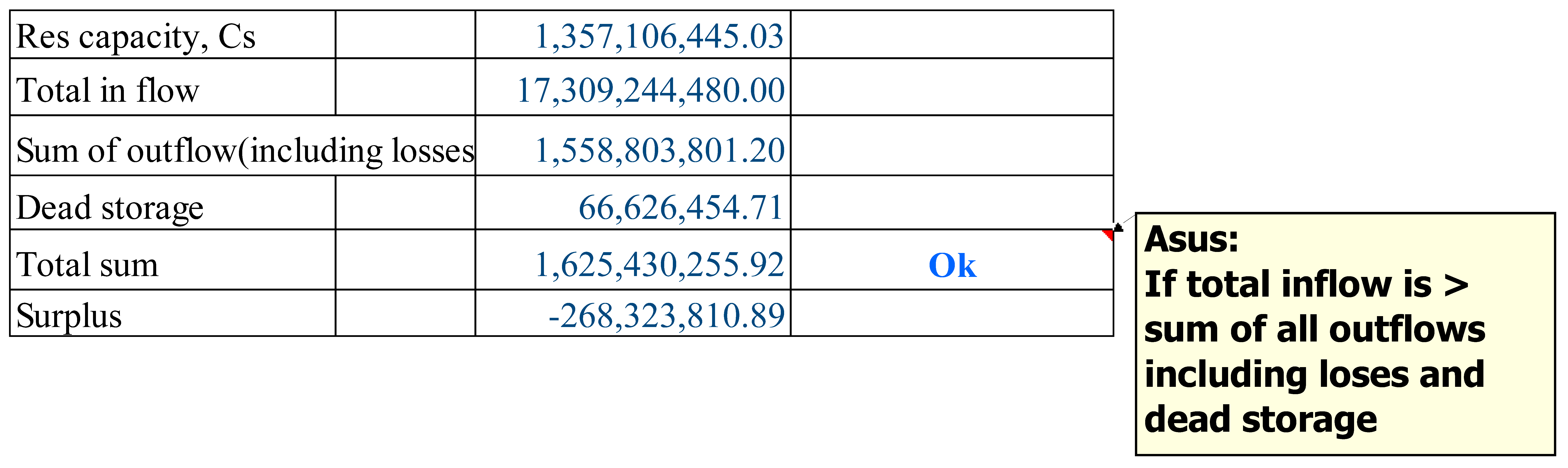
Table 4-2.
Summary of Computed reservoir storage capacity.
| S/N | Dam Site | Reservoir Capacity, Mm3 |
|---|---|---|
| 1 | Dam Site H | 1,357.11 |
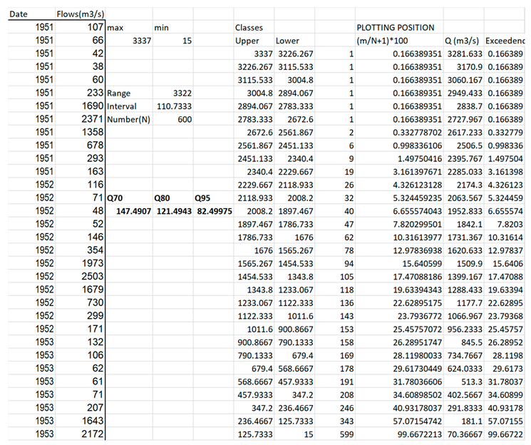
4.4. Downstream release estimation
In order to compute the water balance for further design analyses Q95 is tabulated from the given data for downstream release from the flow duration curve developed[18, 19] and shown in Figure 4-2 and tabulated in Table 4-3 below.
5. Population and Water Supply Demand Estimation
5.1. Population
5.1.1. General
A water supply scheme includes huge and costly structures, which cannot be replaced or increased in their capacities easily and conveniently[20]. Hence all scenarios affecting the water supply system should have to be thoroughly accessed before the system is designed. One of the scenarios that have great impact on estimating the water demand of a particular project is the projection of the population sizes [21]. Hence, the planning of any water supply system has to be based on the forecast of population size, population growth rate and distribution.
There are a number of factors that should be taken in to consideration in projecting the future population size of a project, some of which are fertility, mortality, economic activity in and around the project town, availability of natural resources, and status of the town in the region, i.e. its political and economic significance, relative location of the town with respect to main highways and availability of reliable urban infrastructure facilities and etc [22].
5.1.2. Base Population
The use of a reliable base population figure is very important for optimizing the project costs and sustaining the project’s service year. Over and under estimation of the populations could result in a higher investment cost and a lower service run period respectively. Hence it is very important to initially get a realistic base population figures not to come with the above-mentioned problems. This design has taken the base population of 5 million given for this exercise.
5.1.3. Population Projection
The Central Statistical Authority has established an annual growth rates for population projection from 1995 up to the year 2030. Hence, in projecting the future population sizes of the town and the rural, the country level CSA’s growth rates as presented in the table below have been used. The projected populations using the base populations presented above; and in this report the annual population growth rate is fixed in three scenarios low, medium and high variant. The growth rates presented below are shown in the table and chart presented underneath. For water supply design projects, the medium annual growth rate scenario is adopted.
Figure 5-1.
Population Projection Curve for H project.
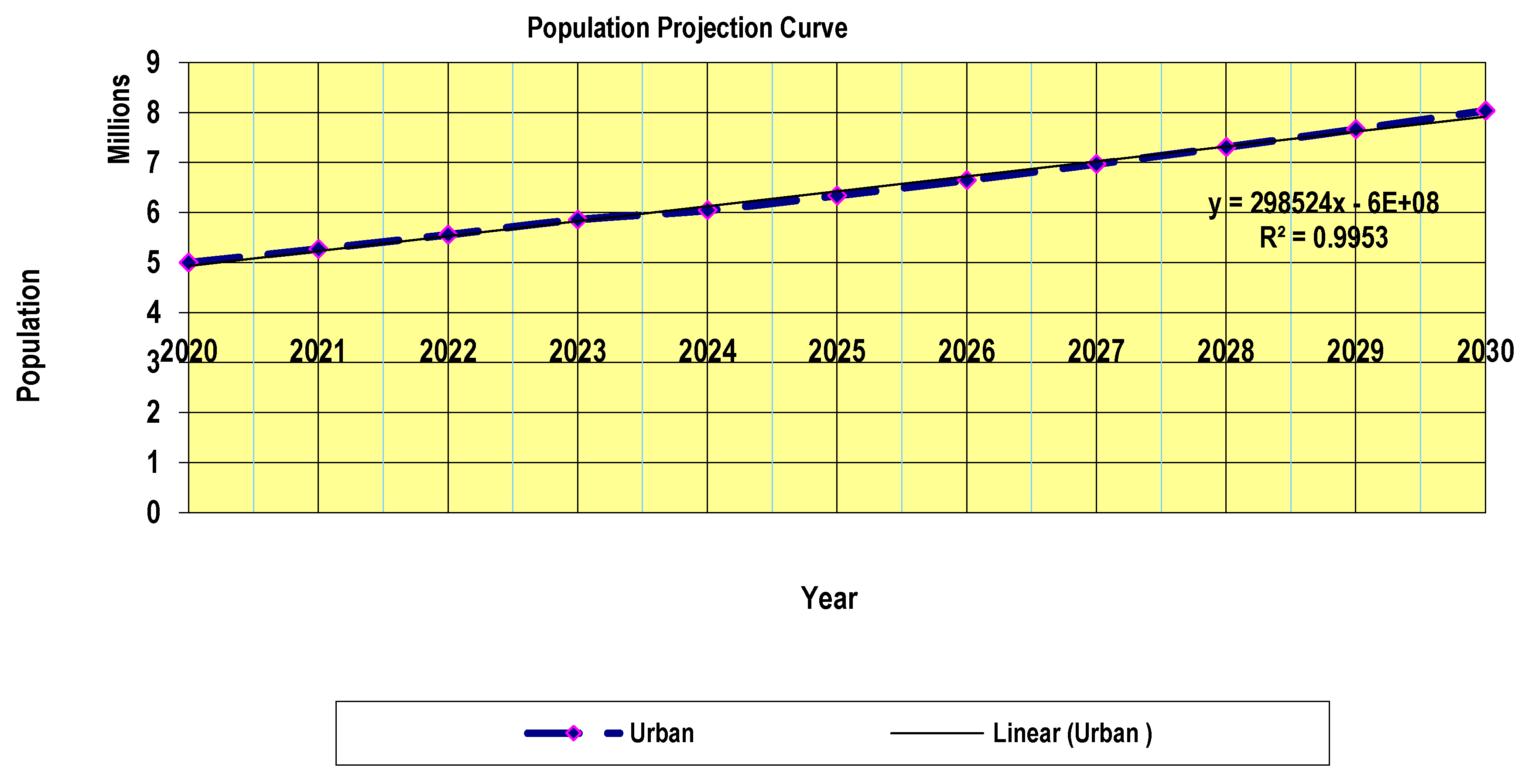
Table 5-1.
Fertility Rate Set by CSA for Urban Population and For Projections.
| Years | Low variants | Medium variants | High variant | Average | Remark |
|---|---|---|---|---|---|
| 1995-2000 | 6.53 | 6.72 | 6.95 | 6.7 | |
| 2001-2005 | 5.28 | 5.97 | 6.72 | 6.0 | |
| 2006-2010 | 4.76 | 5.42 | 6.27 | 5.5 | |
| 2011-2015 | 4.24 | 4.86 | 5.75 | 5.0 | |
| 2016-2020 | 3.8 | 4.29 | 5.22 | 4.4 | |
| 2021-2025 | 3.36 | 3.73 | 4.69 | 3.9 | |
| 2025-2030 | 2.92 | 3.24 | 4.2 | 3.5 |
Table 5-2.
Projected Populations of the given project.
| Years | H project | Rural | Total |
|---|---|---|---|
| 2020 | 5,000,000 | 0 | 5,000,000 |
| 2021 | 5,271,000 | 0 | 5,271,000 |
| 2022 | 5,556,688 | 0 | 5,556,688 |
| 2023 | 5,857,861 | 0 | 5,857,861 |
| 2024 | 6,045,183 | 0 | 6,045,183 |
| 2025 | 6,338,978 | 0 | 6,338,978 |
| 2026 | 6,647,053 | 0 | 6,647,053 |
| 2027 | 6,970,100 | 0 | 6,970,100 |
| 2028 | 7,308,846 | 0 | 7,308,846 |
| 2029 | 7,664,056 | 0 | 7,664,056 |
| 2030 | 8,036,529 | 0 | 8,036,529 |
5.2. Water Demand
Development of reliable water demand is not a straight forward process, but requires detailed socio-economic survey in the supply area, as the potential consumers ability and willingness to pay for the water depends of the tariff, which again depends of the number of people using the improved water supply. The process to develop the demand is hence iterative.
5.2.1. Domestic Water Demand
The Domestic water demand is the daily water requirement for use by human being for different domestic purposes like drinking, cooking, bathing, cleaning, gardening and etc. The domestic water demand required by human being could be supplied or obtained through different modes of services depending on the economic level and facilities owned by the individual.
2.2.1.1. Modes and Level of Services
In a conventional water supply system, there are five modes of services in which an individual could be served. These are:
- House Tap Users [23]
- Yard Tap Users (YTU)
- Neighbor Hood Tap Users (NTU)
- Traditional Sources Users (TSU)
However, in most water supply system feasibility studies for urban centers here in Ethiopia, the modes of services are generally stick to the first three classical modes of services because of their simplicity from the viewpoint of service giving institutions. Hence, for this project, it is assumed all the public to be served by one of the first three modes of services described above.
In estimating the future water demand, it is determined all the rural peoples to be served by public taps as their economic condition doesn’t allow them to use either of the other two modes of services. For the case of this assignment, it is assumed all the three modes of service to prevail and serve the dwellers of the town.
Hence, using the three modes of services namely: Yard Connection, House Connection, and Public Tap and their respective per capita water consumption are described based on the design criteria (willingness and affordability to pay) as stated below: the future water requirement of the town will be estimated in the proceeding section.
- Public Tap users 100litter/day
- Yard Connection 100litter/day
- House Connection 100litter/day
5.2.1.2. Growth Rate of Domestic Water Demand
It is evident that as the socioeconomic condition and the living standard of the people improves; their water consumption will increase depending on their mode of service. The demand of the public tap users will increase very little as the distance involved for fetching water will not encourage the collection of more water and the collection time is limited to day time only, as a result the growth rate has been limited here to 1% per annum. For HCU and YCU, the water demand growth rate per annum could be as high as 2% as it is stated in the design criteria.
Using the above assumptions, the projected per capita water demand for the three demand categories over the expected design period is given in the table hereunder.
5.2.1.3. Projected Level of Service
The percentage of population to be served by each demand category will vary with time. The variation is caused by changes in living standards, improvement of the Service level and the capacity of the water supply service.
Although the standard approach of projecting would normally involves a detail analysis of past consumption trends by consumers group to which alternative economic development scenarios would be applied to produce future consumption levels, this approach requires detail information on the present consumption pattern and future economic development scenarios, which is difficult to get for H town with limited water supply system in the past. However, for this exercise estimation of percentages of each demand category is assumed.
As per the assumption from the willingness and affordability to pay, 50% of the population needs to be served by public taps, 40% of the population need to be served by yard tap connection and 10 % needs to be served house connection.
Table 5-3.
Percentage of Population by Mode of Services in the (2007).
| Mode of Service | Percentage of population |
|---|---|
| House Tap Users | 10.00 |
| Yard Tap Users | 40.00 |
| Public Tap Users | 50.00 |
| Total | 100.00 |
The percentage of population to be served by each demand category is therefore, estimated taking the condition stated above as well as to consider the impact of increasing tariff rate on demand for the future; and assuming that the percentage for the yard taps users and the house tap users will increase gradually during the project service period while that of the public tap users will reduce as people shift to the next demand category. This is because of the expectation that the economic and living standard of the town will increase in the future. Those who previously using public tap will shift their mode of service to either yard connection or house connection.
Figure 5-2.
Percentage of population served by each demand category.
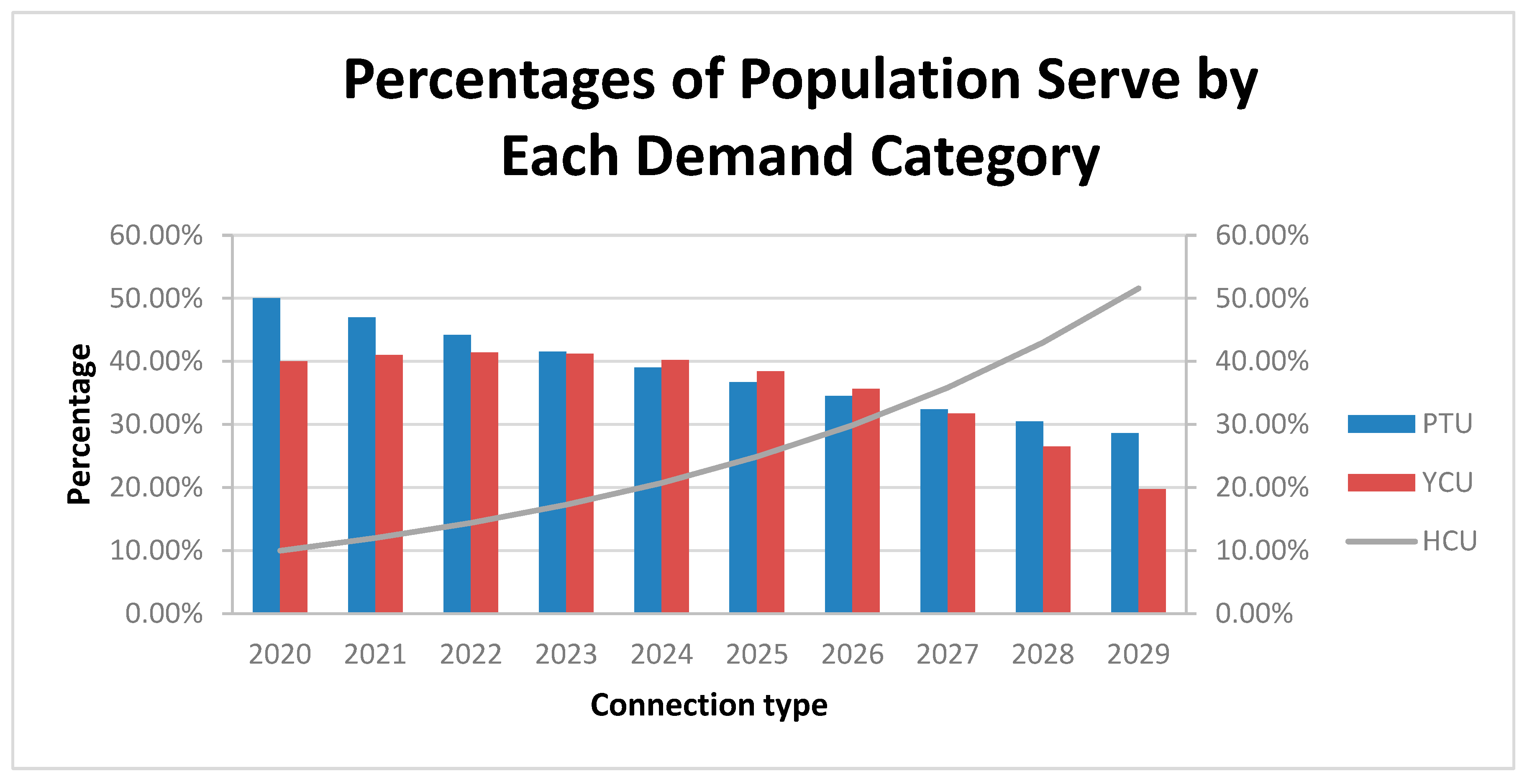
Table 5-4.
Percentages of Population Served by each demand Category (%).
| Demand Category | Year | |||||||||
|---|---|---|---|---|---|---|---|---|---|---|
| 2020 | 2021 | 2022 | 2023 | 2024 | 2025 | 2026 | 2027 | 2028 | 2029 | |
| PTU | 50% | 47% | 44.% | 41.5% | 39.% | 36.7% | 34.5% | 32.4% | 30.5% | 28.6% |
| YCU | 40% | 41% | 41.4% | 41% | 40.2% | 38.4% | 35.6% | 31.7% | 26.5% | 19.7% |
| HCU | 10% | 12 % | 14.4% | 17.3% | 20.74% | 24.9% | 29.8% | 35.8% | 43% | 51.6% |
| Total | 100% | 100% | 100% | 100% | 100.% | 100% | 100% | 100% | 100% | 100% |
5.2.1.4. Projected Per capita Average Domestic Water Demand
The projected per capita average domestic water for a particular year is obtained by multiplying the per capita demand in each category for the year under consideration obtained from Table 4-5 with the corresponding population figure for the same year obtained from Table 4-3 and summing the results for all the demand categories. The proceeding tables show the projected per capita average domestic water demand for H project.
Table 5-5.
Projected Average per capita Domestic Water Demand for H project town.
| Year | 2020 | 2021 | 2022 | 2023 | 2024 | 2025 | 2026 | 2027 | 2028 | 2029 |
|---|---|---|---|---|---|---|---|---|---|---|
| Demand (l/c/d) | 100.0 | 101.5 | 103.1 | 104.8 | 106.6 | 108.5 | 110.4 | 112.4 | 114.5 | 116.6 |
5.2.1.5. Climatic Grouping
In addition to the already discussed factors which influence the quantity of water consumption, climatic of the area is also directly related to the consumption and for this reason, the design criteria consider three climatic group[24, 25]. Hence to consider climatic conditions, factors are adopted and applied to the average demands obtained from Table 4-8. The climatic grouping and corresponding factors are shown in Table 4-9 below.
Table 5-6.
Climatic Grouping.
| Group | Mean annual Precipitation | Factor |
|---|---|---|
| A | <600 | 1.1 |
| B | 601-900 | 1.0 |
| C | >900 | 0.9 |
From the hydro-metrological data, H project has a mean annual rainfall of 1248 mm. Therefore, a climatic adjustment factor of 0.9 is used to adjust the per capita average domestic water demand.
5.2.1.6. Socio-Economic Adjustment Factor
The Socio-economic condition of a town also plays a role in determining the water consumption of an individual town. The design criteria provide for this in the form of categories for the various degrees of development. It is however difficult to quantify many aspects of development and consequently the classification of particular town is made relatively to the others.
Hence, the socioeconomic adjustment factor is determined based on the degree of the development of the particular town under study. The determination of the degree of the existing development and future potential of the town depend on personal judgment due to difficult conditions in quantifying them in short time. The town of H project for this exercise i.e. town under normal Ethiopian condition is asumed. Therefore, socioeconomic adjustment factor of 1.00 is adopted. Table 4-10 below shows the factors of socioeconomic grouping.
Table 5-7.
Socio-Economic Grouping Factor.
| Group | Description | Factor |
|---|---|---|
| A | Towns enjoying high living standard and with very high potential for development | 1.10 |
| B | Towns having a very high potential for development but lower living standard at present | 1.05 |
| C | Towns under normal Ethiopian Condition | 1.00 |
| D | Advanced Rural town | 0.90 |
Applying the climatic and socio-economic adjustment factors to the average domestic water demand calculated in Table 4-8 above, the adjusted average daily domestic water demand for H project town is shown in the Table 4-11 below.
Table 5-8.
Adjusted Average Daily per Capita Demand for H project Town.
| Year | 2020 | 2021 | 2022 | 2023 | 2024 | 2025 | 2026 | 2027 | 2028 | 2029 |
|---|---|---|---|---|---|---|---|---|---|---|
| Average per capita demand l/c/d | 100.00 | 101.53 | 103.14 | 104.84 | 106.61 | 108.46 | 110.39 | 112.39 | 114.46 | 116.60 |
| Climatic adjustment factor | 1 | 1 | 1 | 1 | 1 | 1 | 1 | 1 | 1 | 1 |
| Socio-economic adjustment factor | 1 | 1 | 1 | 1 | 1 | 1 | 1 | 1 | 1 | 1 |
| Adjusted per capita demands l/c/d | 100.00 | 101.53 | 103.14 | 104.84 | 106.61 | 108.46 | 110.39 | 112.39 | 114.46 | 116.60 |
5.2.1.7. Summary of Projected Population and Growth in Domestic Water Demand by Mode of Service
Table 5-9 here under shows summary of population projection; percentages of population served by different modes of service, water demand determination and its growth in the expected service year of the new system are also indicate the calculated adjusted average domestic water demand.
5.2.2. Public Water Demand
The Water required for schools, hospitals, hotels, public facilities, parks, offices, commercial establishments, military camps, small-scale industries and etc. are included in this demand category. Public demand is usually expressed as a percentage of the average day domestic demand.
The general situation related to the public demand is that it is high at the initial stage of the service installation and gradually reduces as the number of connections increase. It is also understood that the percentage of public demand is high in smaller towns as compared to large towns where there could be high number of domestic connections.
The studies in towns having metered water supply system shows that the public water demand ranges between 10 to 20% of domestic consumption depending on the size of the town, type and extents of commercial, economic and industrial activities[26]. For this town, it is considered adequate to assume public demand to be 10% of domestic demand. Table 4-13 below presents the estimated public water demand.
Table 5-10.
Public Water Demand as % of Domestic Water Demand.
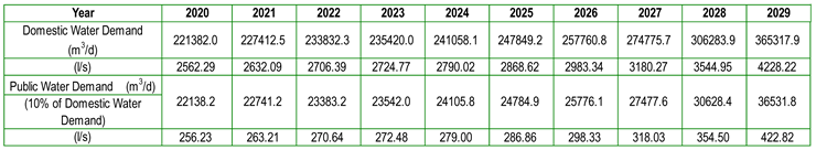 |
5.2.3. Livestock Water Demand
As it is well known, the H project town a town Therefore, the inclusion of the livestock water demand is not obligatory.
5.2.4. Industrial Water Demand
The establishment of an industry is very rare at H project and hence the industrial water demand is not accounted. Even if there could be some industrial development in the future, which is beyond cottage industries, it has to develop its own water supply system not to compete with the new system and impose a higher tariff rate for the customers. Industries, which require water only for domestic use, could take water from the town system and this demand has already been covered under the public water demand.
5.2.5. Water Requirement for Fire Fighting
No extra capacity for firefighting to be considered in small to medium size towns. In case of fire, water required shall be met by stopping supply to consumers for the required time.
5.2.6. Unaccounted for Water [27]
All the water that goes in the distribution pipe does not reach the consumer. Some portion of this is wasted in the pipelines due to defective pipe joints, cracked and broken pipes, faulty valve and fittings. Some consumer keep open their taps or public taps even when they are not using the water and allow continuous wastage of water which also includes illegal connection, unmetered usages such as flushing, firefighting, cleaning the system and overflow from components of the water supply system and etc.
To calculate the future distribution loss it is considered appropriate to relate the percentage of losses to both the age of the distribution system and to the percentage of the total pipeline length, which made up the new distribution system. Water loss relationship curve, which had been adopted by Alexander GIBB’S in 12 towns’ water supply study and from the records of the Water Service office of the town, is utilized in this study to estimate the future water loss of the system. Accordingly, the loss coefficients used for the entire design horizons of the system are presented in the table below.
Table 5-11.
Water Losses Coefficient.
| Year | 2020 | 2021 | 2022 | 2023 | 2024 | 2025 | 2026 | 2027 | 2028 | 2029 |
|---|---|---|---|---|---|---|---|---|---|---|
| % of losses | 20% | 21% | 21% | 22% | 22% | 23% | 23% | 24% | 24% | 25% |
5.2.7. Average Day Demand
The average day water demand is the sum of adjusted domestic water demand, non-domestic water demand and system water loss. The values calculated in the previous sections are summarized and added to estimate the total average day water demand of the project as shown in the Table 4-15 hereunder.
Table 5-12.
Summary of Average Day Water Demand.
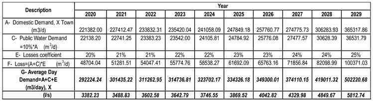 |
*Note: it is assumed major loss to occur in the distribution pipeline only.
5.2.8. Variations of Water Use
The rate of water demand keeps changing from season to season, from day to day and from hour to hour. In hot season, more water is consumed for drinking, bathing and washing clothes than in wet season. The consumption of water is high at weekends and holidays than on normal days, and also more water is required in morning and evening than early in the afternoon and late at night. Therefore, to account these fluctuating water demands, it is necessary to step up the average day demand by certain factor to get the maximum day demand and the peak hour demand. These scaled up water demand figure are used to design the capacities of pumping station, rising main and distribution network.
5.2.8.1. Maximum Day Water Demand
The maximum day water demand is the highest demand of any one 24-hour period over any specified year. If there is sufficient water and enough daily consumption record, it is possible to assume a realistic maximizing factor, however, since there is no any conventional water supply system in the past, the maximizing coefficient are taken from the design guideline of Cost effective Water Supply and Sanitation Project, and are presented on Table 4-16 below.
Table 5-13.
Maximum Day Factor.
| Population | Maximum Daily coefficient (Cd max.) |
|---|---|
| 0-50,000 | 1.2 |
| 50,000-100,000 | 1.15 |
| >100,0000 | 1.1 |
From Table 5-13 and the calculated average day water demand, the maximum daily coefficient to be adopted for H project town and the calculated maximum day demand is presented on Table 5-14 below.
Table 5-14.
Maximum Day Water Demand for H project Town.
| Year | Average Day water Demand | Maximum Day Coefficient (Cd max.) | Maximum Day Demand | |
|---|---|---|---|---|
| (m3/d) | m3/d | l/s | ||
| 2020 | 292224.24 | 1.2 | 350669.09 | 4058.67 |
| 2021 | 301435.22 | 1.2 | 361722.27 | 4186.60 |
| 2022 | 311262.95 | 1.2 | 373515.54 | 4323.10 |
| 2023 | 314736.81 | 1.2 | 377684.17 | 4371.34 |
| 2024 | 323702.17 | 1.2 | 388442.60 | 4495.86 |
| 2025 | 334326.18 | 1.2 | 401191.42 | 4643.42 |
| 2026 | 349300.01 | 1.2 | 419160.01 | 4851.39 |
| 2027 | 374110.15 | 1.2 | 448932.18 | 5195.97 |
| 2028 | 419011.32 | 1.2 | 502813.58 | 5819.60 |
| 2029 | 502220.68 | 1.2 | 602664.81 | 6975.29 |
5.2.8.2. Peak Hour Demand
The peak hour demand is the highest demand in any one hour over the year. It represents the diurnal variation in water demand resulting from behavioral patterns of the local population.
The size, mode of service and social activities of the town significantly influence the peak hour demand. Further, studies show that the peak hour factor is greater for smaller population than bigger population. A peaking factor suiting the town is selected from the design criteria correlating peaking factor with number of population as stated in the table below.
Table 5-15.
Peak Hour Factor.
| Town Population | Peak Hour Factors |
|---|---|
| 0-10,000 | 2.5-3.0 |
| 10,001 - 50,000 | 2.0-2.2 |
| 50,001-100,000 | 1.8 |
| >100,000 | 1.6 |
Hence, since the population of H project town is in the range of >100,000 up to the end of the design period, a peaking factor of 1.6 is adopted to estimate the peak hour demand of the town.
5.2.9. Summary of Water Demand
The calculated water demands are summarized in the form tables and Charts as shown hereunder.
Table 5-16.
Summary of Water Demand.
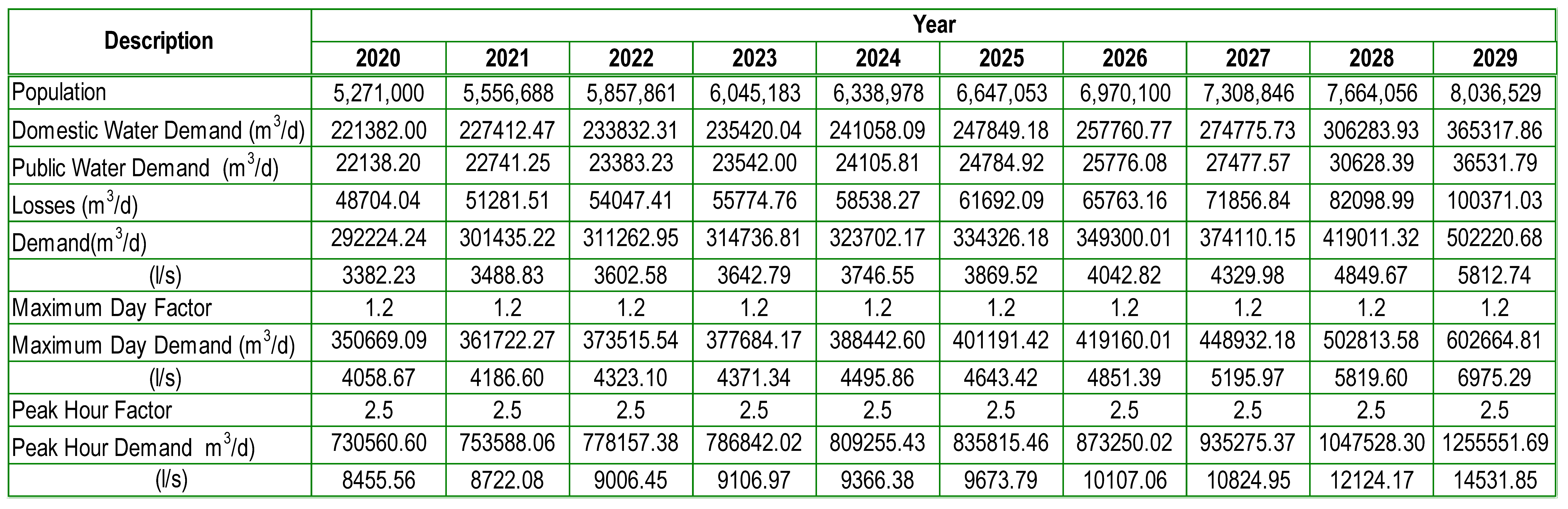 |
Table 5-17.
Summary of Total Water Demands.
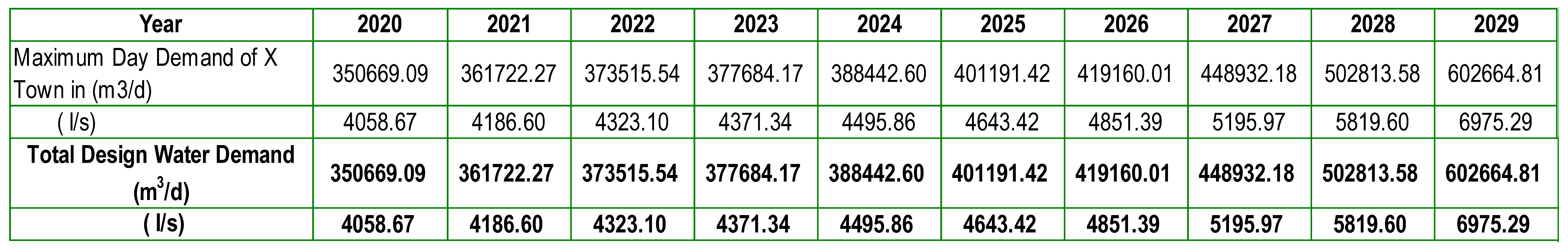 |
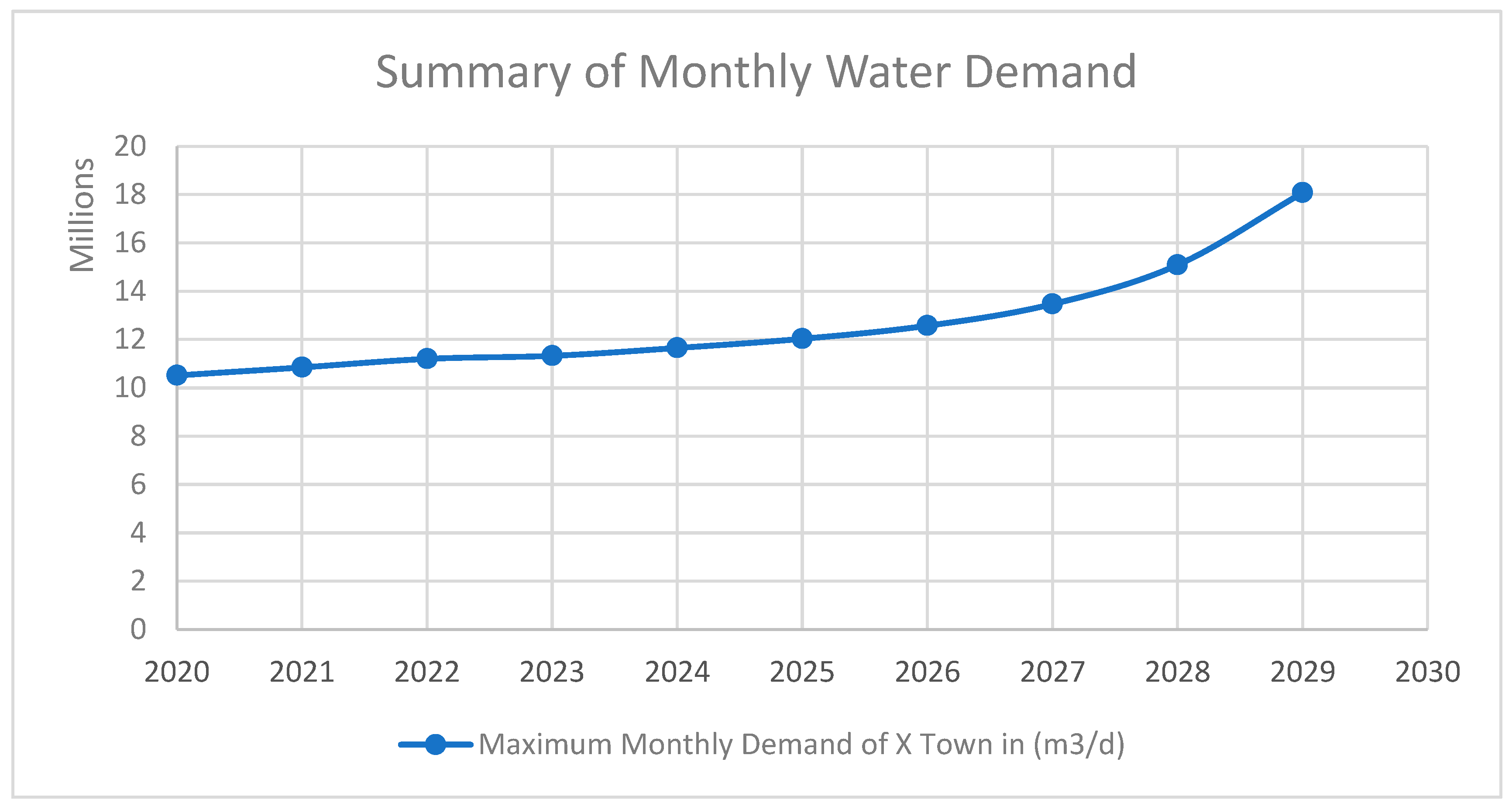
Table 5-18.
Summary of Total Monthly Water Demands.
 |
Figure 5-3.
Summary of monthly water demand. NB: This monthly water demand analyses at the end of first phase of water supply system at year 2030 will be used for water balance analyses this project.
Figure 5-3.
Summary of monthly water demand. NB: This monthly water demand analyses at the end of first phase of water supply system at year 2030 will be used for water balance analyses this project.
6. Irrigation Potential Estimation and Water Demand Analyses
The irrigation potential for this assignment is estimated from the water balance analyses tabulated in table below as per the give data in Table 4-2.
The first step is to calculate the water requirement of the given data by summing up the loss (Etc m3/ha) and the irrigation requirements in to daily bases as shown in table below[9]. Then after, the daily irrigation water requirement will be tabulated again in to total monthly water demand per hectare analyses as shown in table. Therefore, finally the irrigation potential is set by try and error / goal seek approach in excel to estimate the total irrigable command area. Accordingly, the irrigable area is estimated to be 23,500ha as tabulated in water balance analyses.
Table 6-1.
Summary of Total Water Demand for all Crops per hectare.
| S/N | Crop | Planting Date | Growing period (days) | Daily Irrigation water req. (m3/ha) | Irrigation water req. in the specified month(m3/ha) |
|---|---|---|---|---|---|
| 1 | Onion | 01-Feb | 30 | 93.16 | 2794.74 |
| Onion | March | 30 | 93.16 | 2794.74 | |
| Onion | April | 30 | 93.16 | 2794.74 | |
| Onion | May | 5 | 93.16 | 465.79 | |
| 2 | Tomato | 01-Jan | 30 | 97.03 | 2911.03 |
| Tomato | Feb | 30 | 97.03 | 2911.03 | |
| Tomato | March | 30 | 97.03 | 2911.03 | |
| Tomato | April | 30 | 97.03 | 2911.03 | |
| Tomato | May | 25 | 97.03 | 2425.86 | |
| 3 | Wheat | 15-Jan | 15 | 88.68 | 1330.15 |
| Wheat | Feb | 30 | 88.68 | 2660.31 | |
| Wheat | March | 30 | 88.68 | 2660.31 | |
| Wheat | April | 30 | 88.68 | 2660.31 | |
| Wheat | May | 25 | 88.68 | 2216.92 | |
| Total water irrigation requirement per hectare | 34,448.00 | ||||
Table 6-2.
Summary of Total Monthly Water Demand for all Crops for the optimum hectare.
| S/N | Month | Planting Date | Irrigation water req. per month (m3/ha) | Irrigation water req. for 23,500 ha |
|---|---|---|---|---|
| 1 | Jan | Jan | 4,241.19 | 99,667,925.73 |
| 2 | Feb | Feb | 8,366.08 | 196,602,856.90 |
| 3 | March | March | 8,366.08 | 196,602,856.90 |
| 4 | April | April | 8,366.08 | 196,602,856.90 |
| 5 | May | May | 5,108.57 | 120,051,503.56 |
| Total Project Monthly Irrigation Water Demand for Water Balance Analyses | 809,528,000.00 | |||
Table 6-3.
Runoff coefficient calculator.
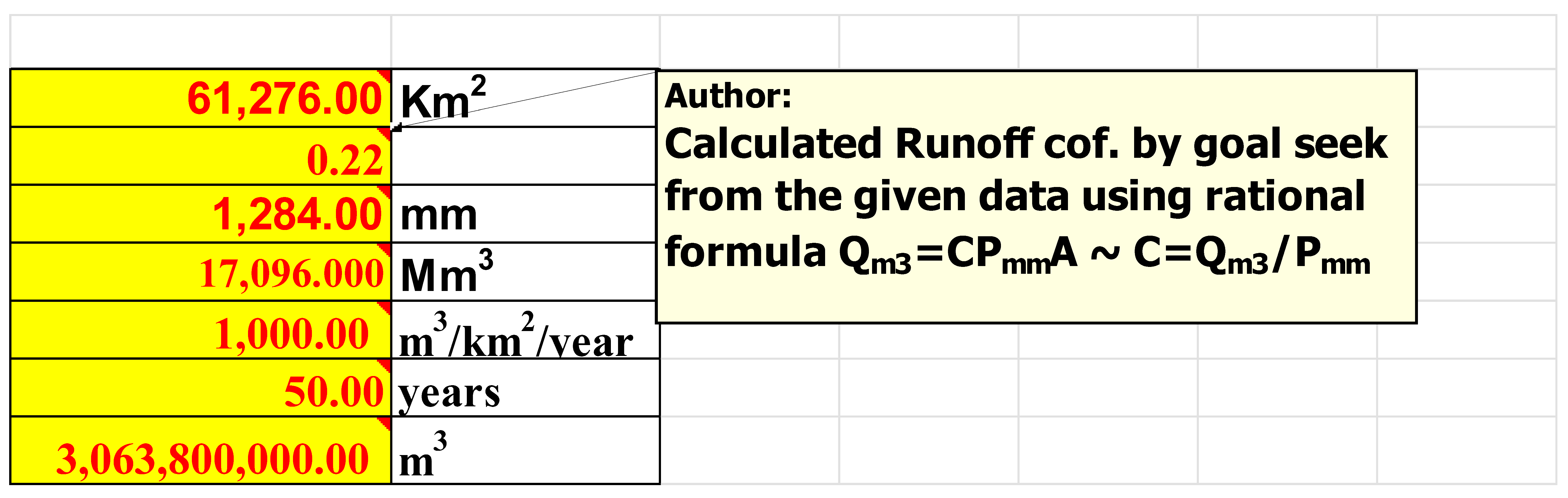 |
Table 6-4.
Water Balance Sheet.
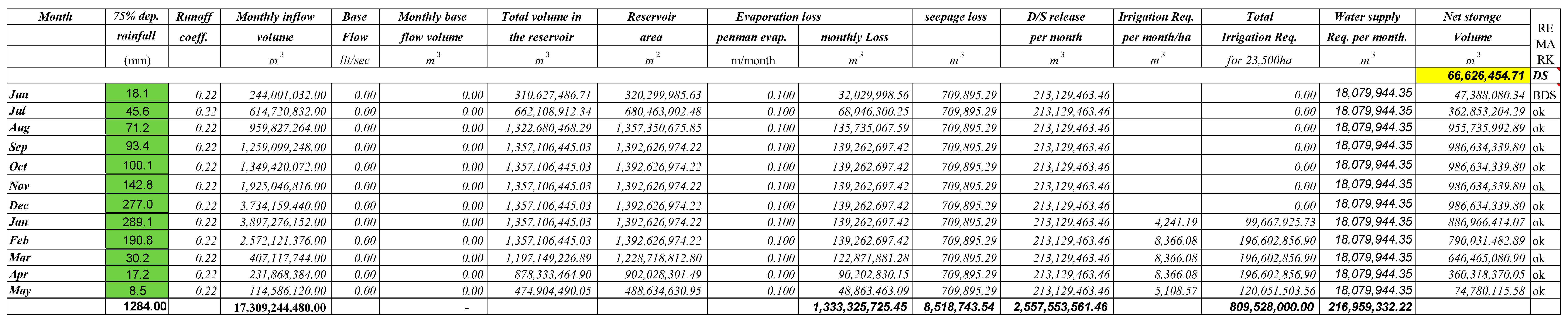 |
Table 6-5.
Reservoir Characteristics.
 |
7. Hydropower Potential and Energy Generation
7.1. Energy of Hydropower
7.1.1. Hydropower Generation
The waters of lakes, reservoirs located at high elevation and water flowing in a river all provide potential energy or kinetic energy[28]. The energy produced by water is termed water power. Power generation methods which produce electric energy by using water power are called hydropower generation.
7.1.2. Electric Power Output
Hydro power plants are equipped with turbines and generators which are turned by water power to generate electric power[29]. Here, the water power is first converted into mechanical energy then into electric energy. In this form of energy conversion process, there is a certain amount of energy loss due to the turbine and generator. The power output is expressed by the following equation.
P=ρ9.8QHe
Where
P: Power output(kW)
ρ: Water density = 1,000kg/m3 (at 4 ºC, elevation 0m and 1atm)
9.8: Approximate value of free fall acceleration/sec2)
Q: Power discharge (m3/sec )
He: Effective head (m)
η: Combined efficiency of turbine and generator
The MW unit is also used to express the power output. 1,000 kilowatt (kW) is equal to 1 megawatt (MW.
Maximum output1, rated output, firm output, and firm peak output are used to express the performance of the power plant.
7.1.3. Energy Generation
Power output (P) is the magnitude of the electric power generated. The electric energy generated by continuous operation of P (kW) for T (hours) is termed generated energy and is expressed by kilowatt hour (kWh).
The following Table 7-1 shows the discharge taken from water balance analyses. Therefore, according to the topography condition the following discharges can be used for hydropower development plant. However, for the illustration of this example only downstream release for power generation is taken.
Table 7-1.
Outlet discharges for multipurpose reservoir of the project .
| S/N | Description | Discharge in m3/sec |
|---|---|---|
| 1 | Qd/s release | 82.23 |
| 2 | Qirr | 25.32 |
| 3 | Qws | 6.98 |
| 4 | Total | 114.52 |
Hence, according the above formula and the tabulated data in Table 7-1 the design is calculated as follows:
Where,
KW = 9.81 x Q x H x η
KW = electric power in kW
Q = quantity of water flowing through the hydraulic turbine in cubic meters per second. Discharge (quantity of water) flowing in a stream and available for power generation has daily and seasonal variation. Optimum discharge for power generation is determined on the basis of energy generation cost.
He = Net available head in meters (gross head – losses)
Hd = net head resulting between river-bed and reservoir level =2000m
He = 150 + Hd = 350m
η = overall efficiency of the hydro power plant. For general estimation purposes, η is normally taken as 0.85, a hydropower station has a gross head of He = 150 +Hd meter. Head loss in water conductor system is neglected for this exercise. Optimum discharge in m3 is 82.23 cubic meter per second.
KW = 9.81 x 82.23 x 350 x 0.85
KW = 239,974.16
MW = 240
Energy generation E = average power x 24 x 365 in (MWh) units= 2,102,400.00
Accordingly 3 units of 3 x 80 MW can be installed.
8. Frequency Analyses and Flood Routing
8.1. Introduction
Flood routing is the technique of determining the flood hydrograph at a section of a river by utilizing the data of flood flow at one or more upstream sections [30]. The hydrologic analysis of problems such as flood forecasting, flood protection, reservoir design and spillway design invariably include flood routing. In these applications two broad categories of routing can be recognized. These are reservoir routing and channel routing. In reservoir routing the effect of a flood wave entering a reservoir is studied. In channel routing the change in the shape of a hydrograph as it travels down a channel is studied. In this project a flood frequency analyses and reservoir routing is undertaken to see the behaviour of the reservoir while incoming the design flood (peak flood) under certain return period 100, 500 and 1000 years return period[31].
The term flood routing refers to procedures to determine the outflow hydrograph at a point downstream in a river (or reservoir) as a function of the inflow hydrograph at a point upstream. As flood waves travel downstream they are attenuated and delayed. That is, the peak flow of the hydrograph decreases and the time base of the hydrograph increases. Again design flood is the flood discharge adopted for the design of a structure after careful consideration of economic and hydrologic factors. As the magnitude of the design flood increases, the capital cos t of the structure also increases but the probability of annual damages will decrease.
8.2. Reservoir routing
Let I and Q be the inflow into and outflow from a reservoir, and S the storage in the reservoir, the continuity equation in the differential form for the reservoir[32] is given by
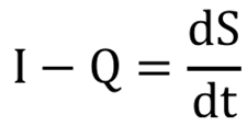 Equation 8-1
Alternatively, the same can be written as
 Equation 8-2
Where, I is the average inflow rate in a small time interval ∆t , Q is the average outflow rate in the same time interval and ∆S is the corresponding change in the storage of the reservoir during the same time interval. If suffixes 1 and 2 are used to denote a given quantity at the beginning and the end of the time interval and if the inflow and outflow have straight line variation within the time interval, Eq. (2) can be written as
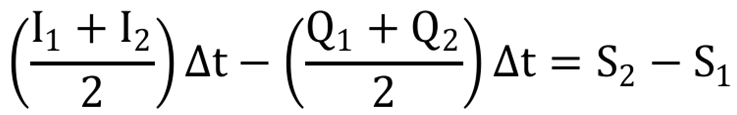 Equation 8-3
8.3. Design flood
Flood is the unusual high stage of a river due to runoff from rainfall and or melting of snow in quantities too great to be confined in the normal water surface elevations of the river or stream, as the result of unusual meteorological combination[33]. The maximum flood that any structure can safely pass is called the ‘Design flood’ and is selected after consideration of economic and hydrologic factors. The design flood is related to the project feature and may be arrived by considering the cost of constructing the structure to provide flood control and the flood control benefits arising directly by prevention of damage to structures downstream, disruption communication, loss of life and property, damage to crops and under -utilization of land. The design flood is usually selected after making a cost-benefit analysis and exercising engineering judgment. In general the methods used in the estimation of the design flood can be grouped as below.
(ì) Increasing the observed maximum flood by a certain percentage
(ìì) Envelope curves
(ììì) Empirical flood formulae
(ìv) Rational method
(v) Unit hydrograph application
(vì) Frequency analysis (or Statistical methods)
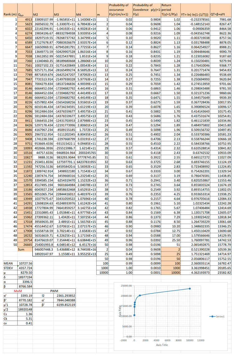
8.4. Frequency analyses
In this project frequency analysis will be used to determine the design flood. The analyses makes use of the observed data in the past to predict the future flood events along with their probabilities or return periods. It is based on the assumption that combination of the numerous factors which produce floods are a matter of pure chance and therefore are subject to analysis according to the mathematical theory of probability.
Figure 8-1.
Flood frequency analyses of different statistical distributions.
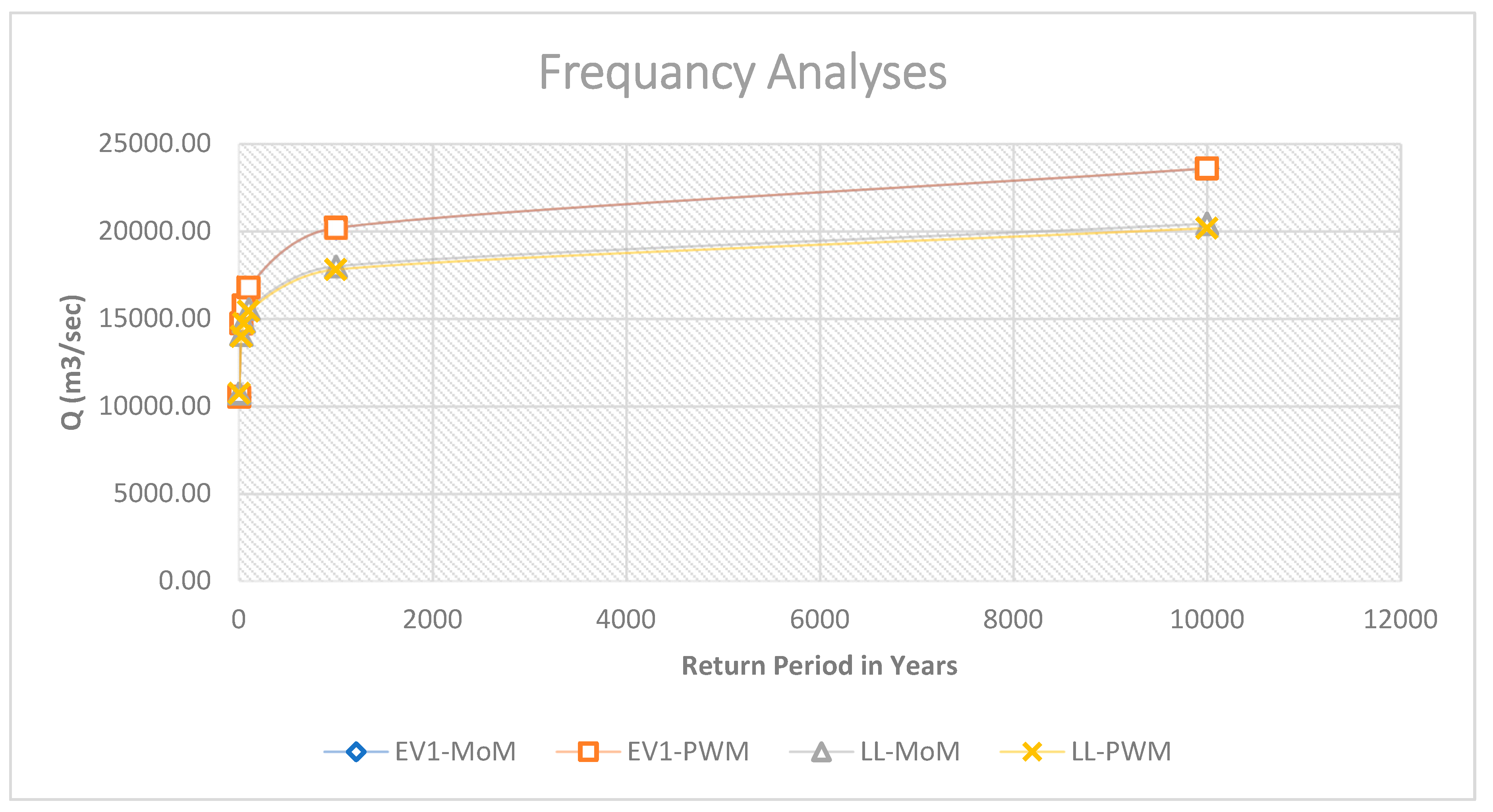
8.5. Flood routing calculation
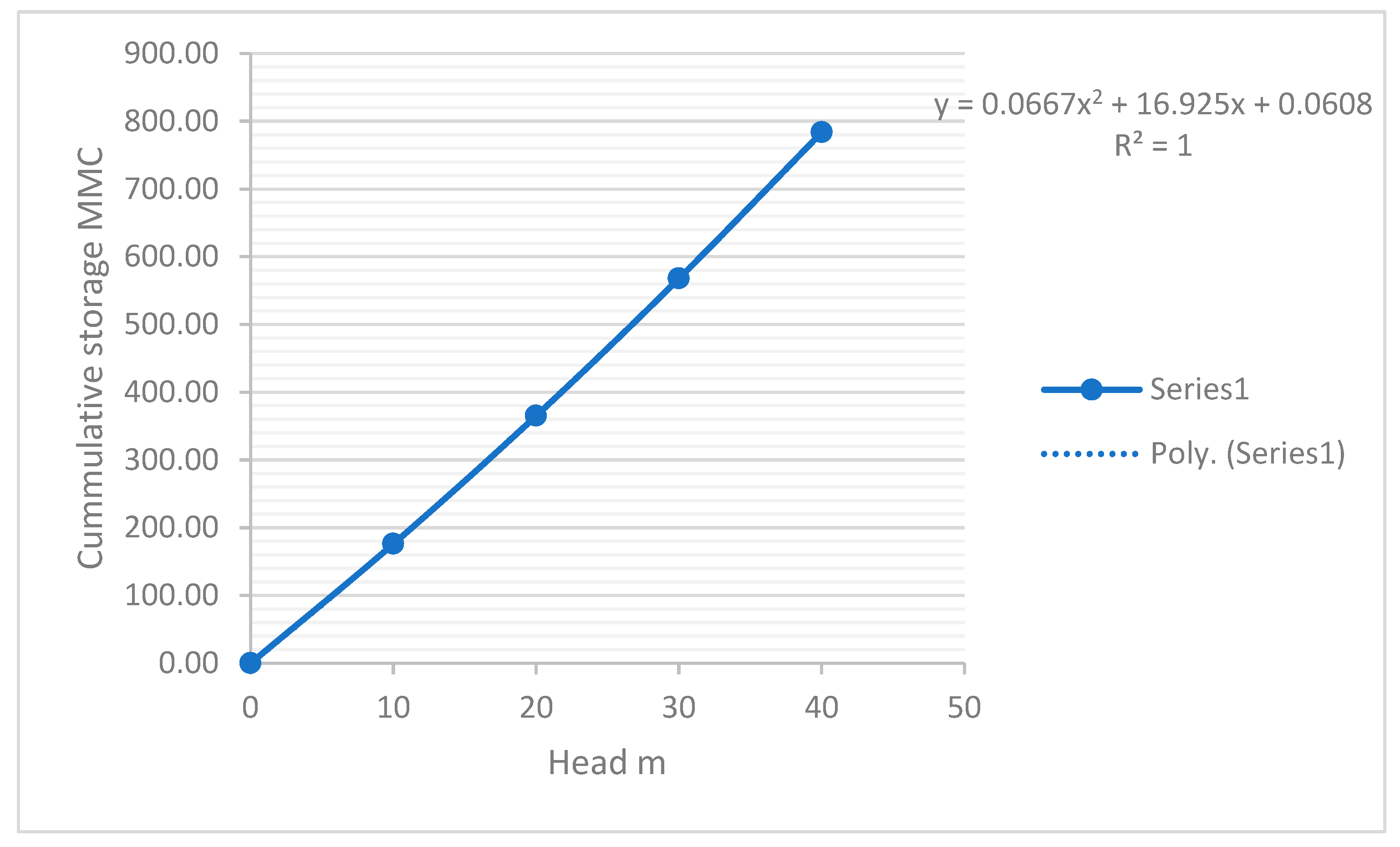
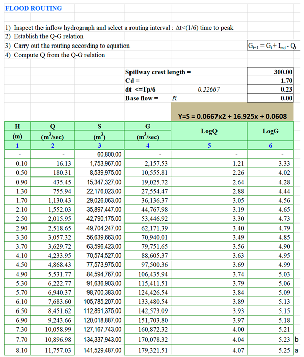
Table and Figure 8-1 shows the relationship between head, discharge and storage of the reservoir above NPL for the analyses of reservoir routing of Table 8-6.
Table 8-1.
Reservoir characteristics above NPL.
| ELEVATION (masl) | TOTAL VOLUME (MMC) | Surcharge Head, H(m) | Storage(MMC) | cumulative Storage(MMC) | Q(m3/s) | 2S/∆t+Q |
|---|---|---|---|---|---|---|
| 1200.00 | 1357.11 | 0 | 0.00 | 0.00 | 0 | 0 |
| 1210.00 | 1533.22 | 10 | 176.11 | 176.11 | 1075 | 432715 |
| 1220.00 | 1722.37 | 20 | 189.15 | 365.26 | 3041 | 898287 |
| 1230.00 | 1924.87 | 30 | 202.50 | 567.76 | 5587 | 1397156 |
| 1240.00 | 2141.02 | 40 | 216.15 | 783.91 | 8601 | 1929948 |
Figure 8-2.
Stage Vs cumulative storage relationship.
Because of data limitation on the project Tc is calculated from the Empirical formula below.
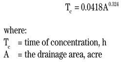 According the above formula a table below is tabulated to calculate Tc and other important parameters as stated below to develop the input hydrograph for flood routing propose. The flow to be routed is also taken from the frequency analyses result of the 1000 and 10000 return period just to see how the damping effect of the reservoir will behave.
According the above formula a table below is tabulated to calculate Tc and other important parameters as stated below to develop the input hydrograph for flood routing propose. The flow to be routed is also taken from the frequency analyses result of the 1000 and 10000 return period just to see how the damping effect of the reservoir will behave.
Table 8-2.
Parameters calculation table.
| Step | Parameter | Unit | Value |
|---|---|---|---|
| 1 | Catchment Area | Km2 | 61276.00 |
| 2 | Length of main | m | |
| water course | |||
| 3 | Time of concentration, Tc | hr | 8.86 |
| 4 | Rain fall excess duration | hr | |
| D = Tc/6 | hr | 1.00 | |
| 5 | Time to peak, Tp | hr | |
| Tp = 0.6 Tc + 0.5 D | hr | 5.82 | |
| 6 | Time to base, Tb | hr | |
| Tb = 2.67 Tp | hr | 15.53 | |
| 7 | Peak rate of discharge created by 1mm runoff excess on whole of the catchment, Tp | m3/sec/mm | |
| p = (0.21* A) / Tp | 2211.96 | ||
| 8 | Lag time, tl | hr | |
| tl = 0.6 Tc | 5.32 |
Table 8-3.
Time of incremental Hydrograph.
| Time of incremental hydrograph | ||
| Time of beginning | Time to Peak | Time to End |
| hr | ||
| 0.00 | 5.8 | 15.5 |
| 1.00 | 6.8 | 16.5 |
| 2.00 | 7.8 | 17.5 |
| 3.00 | 8.8 | 18.5 |
| 4.00 | 9.8 | 19.5 |
| 5.00 | 10.8 | 20.5 |
Table 8-4.
Inflow hydrograph plotting table.
| Incremental run off to develop the complex hydrograph | Time of | Time to | Time to | |
|---|---|---|---|---|
| begin | peak | end | ||
| Tr (Years) | Qp (m3/sec) | hrs | ||
| 0 | 0.00 | 0.00 | 5.82 | 15.53 |
| 25 | 4530.90 | 1.00 | 6.82 | 16.53 |
| 50 | 4850.42 | 2.00 | 7.82 | 17.53 |
| 100 | 5167.59 | 3.00 | 8.82 | 18.53 |
| 1000 | 6215.60 | 4.00 | 9.82 | 19.53 |
| 10000 | 7261.76 | 5.00 | 10.82 | 20.53 |
Table 8-5.
Ordinate of Input hydrograph.
| (hr) | Ordinate of Hydrograph (m3/Sec) | ||||||
| 1 | 2 | 3 | 4 | 5 | 6 | 7 | |
| 0 | 0.00 | 0.00 | |||||
| 1.00 | 0.00 | 0.00 | 0.00 | ||||
| 2.00 | 0.00 | 940.52 | 0.00 | 940.52 | |||
| 3.00 | 0.00 | 1881.04 | 1006.84 | 0.00 | 2887.88 | ||
| 4.00 | 0.00 | 2821.56 | 2013.69 | 1072.68 | 0.00 | 5907.93 | |
| 5.00 | 0.00 | 3762.07 | 3020.53 | 2145.36 | 1290.23 | 0.00 | 10218.20 |
| 5.82 | 0.00 | 4530.90 | 3843.58 | 3022.23 | 2344.92 | 1232.21 | 14973.84 |
| 6.82 | 0.00 | 4064.52 | 4850.42 | 4094.91 | 3635.15 | 2739.60 | 19384.60 |
| 7.82 | 0.00 | 3598.15 | 4351.16 | 5167.59 | 4925.37 | 4246.99 | 22289.26 |
| 8.82 | 0.00 | 3131.77 | 3851.89 | 4635.68 | 6215.60 | 5754.37 | 23589.32 |
| 9.82 | 0.00 | 2665.40 | 3352.63 | 4103.77 | 5575.82 | 7261.76 | 22959.37 |
| 10.82 | 0.00 | 2199.02 | 2853.36 | 3571.86 | 4936.03 | 6514.29 | 20074.57 |
| 15.53 | 0.00 | 499.26 | 1063.82 | 1919.35 | 2989.87 | 6472.31 | |
| 16.53 | 0.00 | 531.91 | 1279.57 | 2242.41 | 4053.89 | ||
| 17.53 | 0.00 | 639.78 | 1494.94 | 2134.72 | |||
| 18.53 | 0.00 | 747.47 | 747.47 | ||||
| 19.53 | 0.00 | 0.00 | |||||
Figure 8-3.
Inflow Hydrograph.
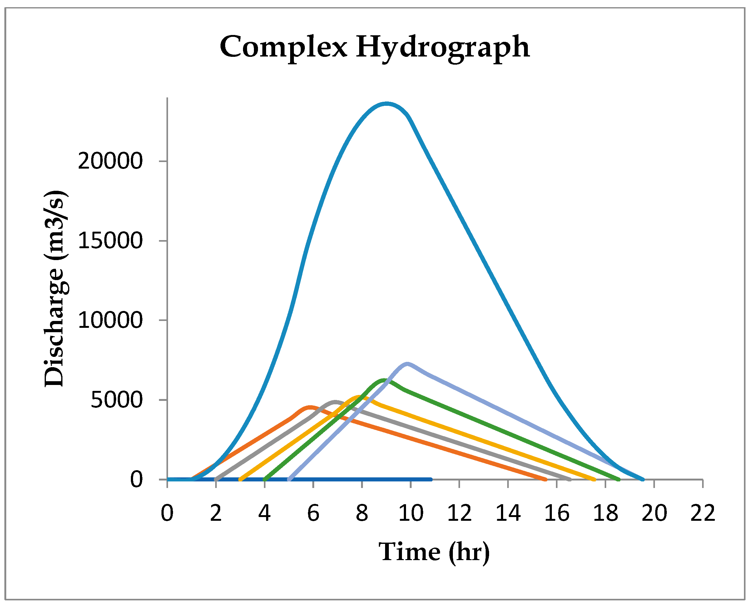
Figure 8-4.
Routed hydrograph.
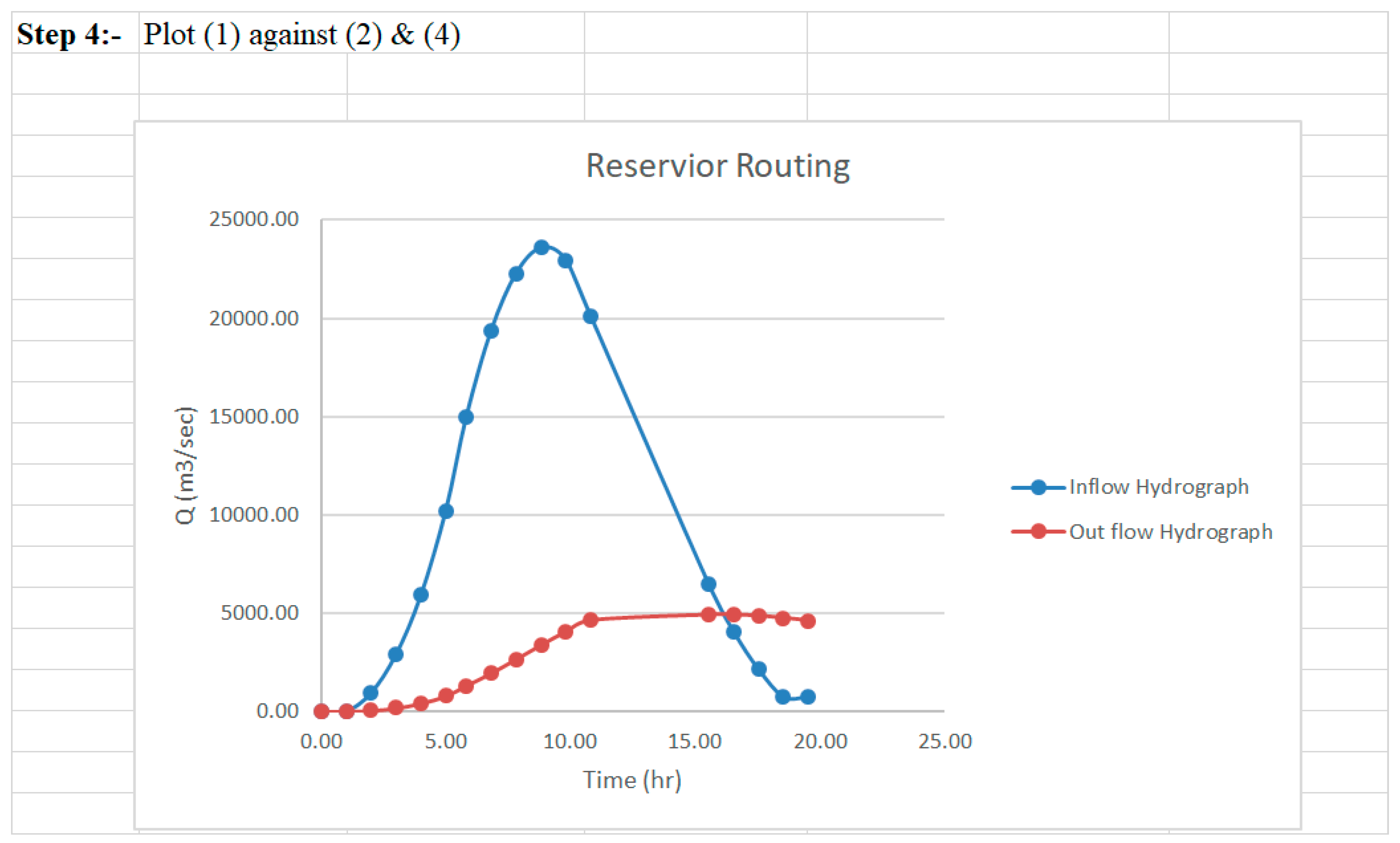
Table 8-6.
Reservoir routing tables.
 |
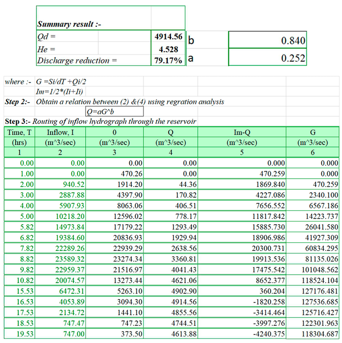 |
Figure 8-5.
Optimum spillway sizing graph.
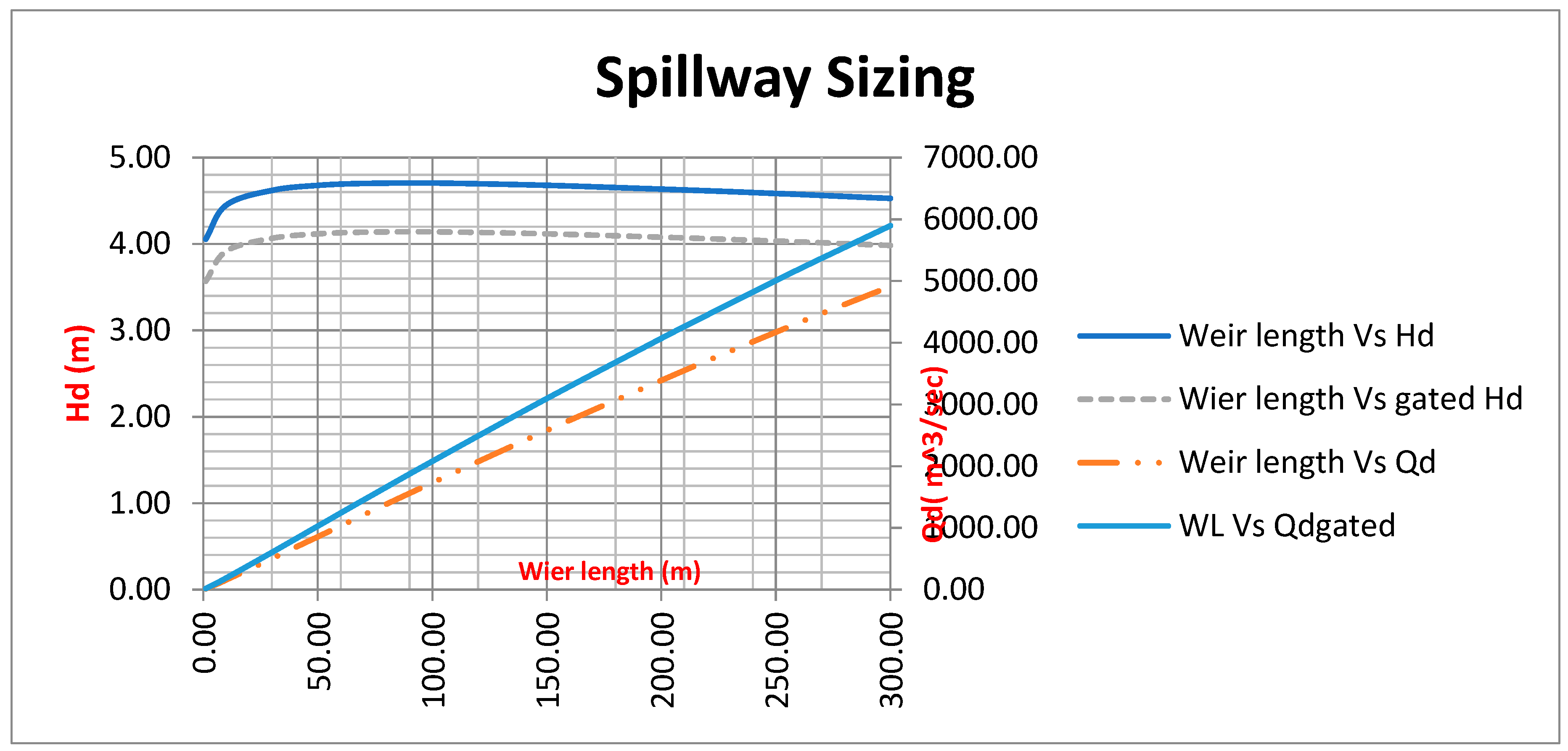
The above Figure 8-5 shows how to size the spillway of the project, however since we don’t have the cost data of the project we cannot be sure to select the optimum one. But, for this this case we can choose the size of the spillway by looking Hd and the design flood magnitude. And, for this exercise it’s routed for 300m spillway width, the point wher Hd & Qd crossed each other. At this stage the damping effect of the reservoir is 79.1% and the design flood of the spillway is selected 4915m3/sec.
9. Conclusions and Recommendation
In conclusion this is a technical note prepared to assist junior young engineers with practical example, and is recommended for those who are engaged in the study and design of stochastic hydrology, spillway, dam, irrigation, water supply and hydropower projects.
10. ANNEX
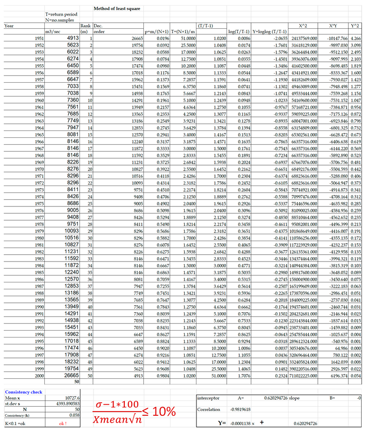
10.1. Annex 10-1 Consistency Test
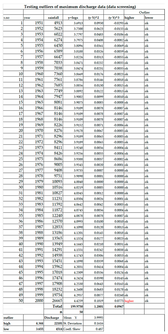
10.2. Annex 10-2 Outliers test
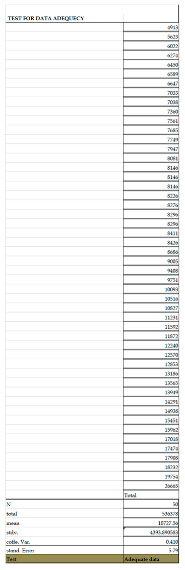
10.3. Annex 10-3 Adequacy test
10.4. Annex 10-4 Flood frequency analyses sheet
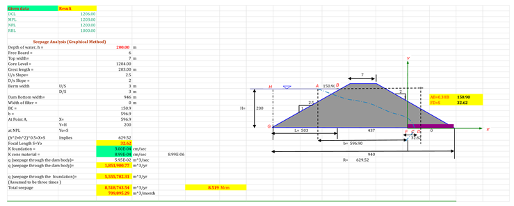
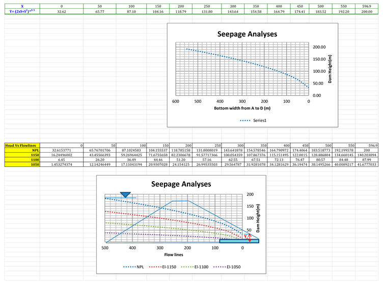
10.5. Annex 10-5 Seepage analyses and frequency analyses tables

Abbreviation
H project means Hiben Project
References
- Hiben MG, Awoke AG, Ashenafi AAJJoG, Cartography. Homogeneity and change point detection of hydroclimatic variables: A case study of the Ghba River Subbasin, Ethiopia. Journal of Geography & Cartography. 2023;6:2010. [CrossRef]
- Hiben MG, Awoke AG, Ashenafi AAJJoAWE, Research. Estimation of rainfall and streamflow missing data under uncertainty for Nile basin headwaters: the case of Ghba catchments. Journal of Applied Water Engineering & Research. 2023:1-15. [CrossRef]
- Sattari M-T, Rezazadeh-Joudi A, Kusiak AJHR. Assessment of different methods for estimation of missing data in precipitation studies. 2017;48:1032-44. [CrossRef]
- Jahan F, Sinha NC, Rahman M, Mondal M, Haque S, Islam MAJT, et al. Comparison of missing value estimation techniques in rainfall data of Bangladesh. 2019;136:1115-31.
- Ismail WW, Zin WZW, Ibrahim WJMJFAS. Estimation of rainfall and stream flow missing data for Terengganu, Malaysia by using interpolation technique methods. 2017;13:214-8.
- Teegavarapu RS, Chandramouli VJJoh. Improved weighting methods, deterministic and stochastic data-driven models for estimation of missing precipitation records. 2005;312:191-206.
- Kizza M, Westerberg I, Rodhe A, Ntale HKJJoH. Estimating areal rainfall over Lake Victoria and its basin using ground-based and satellite data. 2012;464:401-11. [CrossRef]
- Maleika WJAG. Inverse distance weighting method optimization in the process of digital terrain model creation based on data collected from a multibeam echosounder. 2020;12:397-407. [CrossRef]
- Hiben MG, Awoke AG, Ashenafi AAJAJoG, ISSN RP. Assessment of Hydrological and Water management Models for Ghba Subbasin, Ethiopia. J African Journal of Geography. 2023;10:001-7. [CrossRef]
- Loucks DP, Van Beek E. Water resource systems planning and management: An introduction to methods, models, and applications: Springer; 2017.
- Ghaffour N, Missimer TM, Amy GLJD. Technical review and evaluation of the economics of water desalination: Current and future challenges for better water supply sustainability. 2013;309:197-207. [CrossRef]
- Gosschalk EM. Reservoir engineering: guidelines for practice: Thomas Telford; 2002.
- Padmavathy A, Raj KG, Yogarajan N, Thangavel P, Chandrasekhar MJAiSR. Checkdam site selection using GIS approach. 1993;13:123-7. [CrossRef]
- Sherard JLJJotSM, Division f. Earthquake considerations in earth dam design. 1967;93:377-401.
- Thiyagarajan SR, Emadi H, Hussain A, Patange P, Watson MJJoES. A comprehensive review of the mechanisms and efficiency of underground hydrogen storage. 2022;51:104490.
- Tunji LAQ, Sempewo JI, Mbatya WJJoAWE, Research. Development of a water surface area-storage capacity relationship for Namodope Reservoir, Uganda. 2020;8:183-93. [CrossRef]
- Irvem AJIJNES. Application of GIS to determine storage volume and surface area of reservoirs: the case study of Buyuk Karacay dam. 2011;5:39-43.
- Kim J, Lee J, Park J, Kim S, Kim S. Improvement of downstream flow by modifying SWAT reservoir operation considering irrigation water and environmental flow from agricultural reservoirs in South Korea. Water. 2021;13:2543. [CrossRef]
- Abebe WB, Tilahun SA, Moges MM, Wondie A, Dersseh MG, McClain MEJED. Environmental flow assessment and implications on sustainability of aquatic ecosystems in Ethiopia: A literature review on global and national evidences. 2022:100758. [CrossRef]
- Alegre H, Baptista JM, Cabrera Jr E, Cubillo F, Duarte P, Hirner W, et al. Performance indicators for water supply services: IWA publishing; 2016.
- Rosegrant MW, Cai XJWI. Global water demand and supply projections: part 2. Results and prospects to 2025. 2002;27:170-82.
- Smith SK, Tayman J, Swanson DA. A practitioner's guide to state and local population projections: Springer; 2013.
- Alemayehu T, Mebrahtu G, Hadera A, Bekele DNJSWRM. Assessment of the impact of landfill leachate on groundwater and surrounding surface water: a case study of Mekelle city, Northern Ethiopia. 2019;5:1641-9. [CrossRef]
- Hiben MG, Awoke AG, Ashenafi AA. Assessment of Future Water Demand for Resilient Water Allocation under Socioeconomic and Climate Change Scenarios, a Case of Ghba Subbasin, Northern Ethiopia. Preprints. 2023.
- Hiben MG, Awoke AG, Ashenafi AA. Hydroclimatic Variability, Characterization, and Long Term Spacio-Temporal Trend Analysis of the Ghba River Subbasin, Ethiopia. Advances in Meteorology. 2022;2022:3594641. [CrossRef]
- Hiben MG, Gebeyehu AA, Adugna AA, Shang Y. Estimation of Current Water Use over the Complex Topography of the Nile Basin Headwaters: The Case of Ghba Subbasin, Ethiopia. Advances in Civil Engineering. 2022;2022:1-14.
- Hailu R, Tolossa D, Alemu GJSWRM. Water security: stakeholders’ arena in the Awash River Basin of Ethiopia. 2019;5:513-31. [CrossRef]
- Guseva S, Casper P, Sachs T, Spank U, Lorke AJW. Energy flux paths in lakes and reservoirs. 2021;13:3270. [CrossRef]
- Asanov M, Safaraliev MK, Zhabudaev TZ, Asanova S, Kokin S, Dmitriev S, et al. Algorithm for calculation and selection of micro hydropower plant taking into account hydrological parameters of small watercourses mountain rivers of Central Asia. 2021;46:37109-19. [CrossRef]
- Fenton JDJJoH. Flood routing methods. 2019;570:251-64.
- Tarpanelli A, Barbetta S, Brocca L, Moramarco TJRS. River discharge estimation by using altimetry data and simplified flood routing modeling. 2013;5:4145-62. [CrossRef]
- Ahmed T, McKinney P. Advanced reservoir engineering: Elsevier; 2011.
- Hiben MG, Di Baldassarre G, Van Griensven AJEJoWS, Technology. Can We Model Floodplain Inundation Patterns in Data-Scarce Areas? 2020;3:111-29.
Figure 4-1.
Elevation-Area-Capacity Curve for Dam Site.
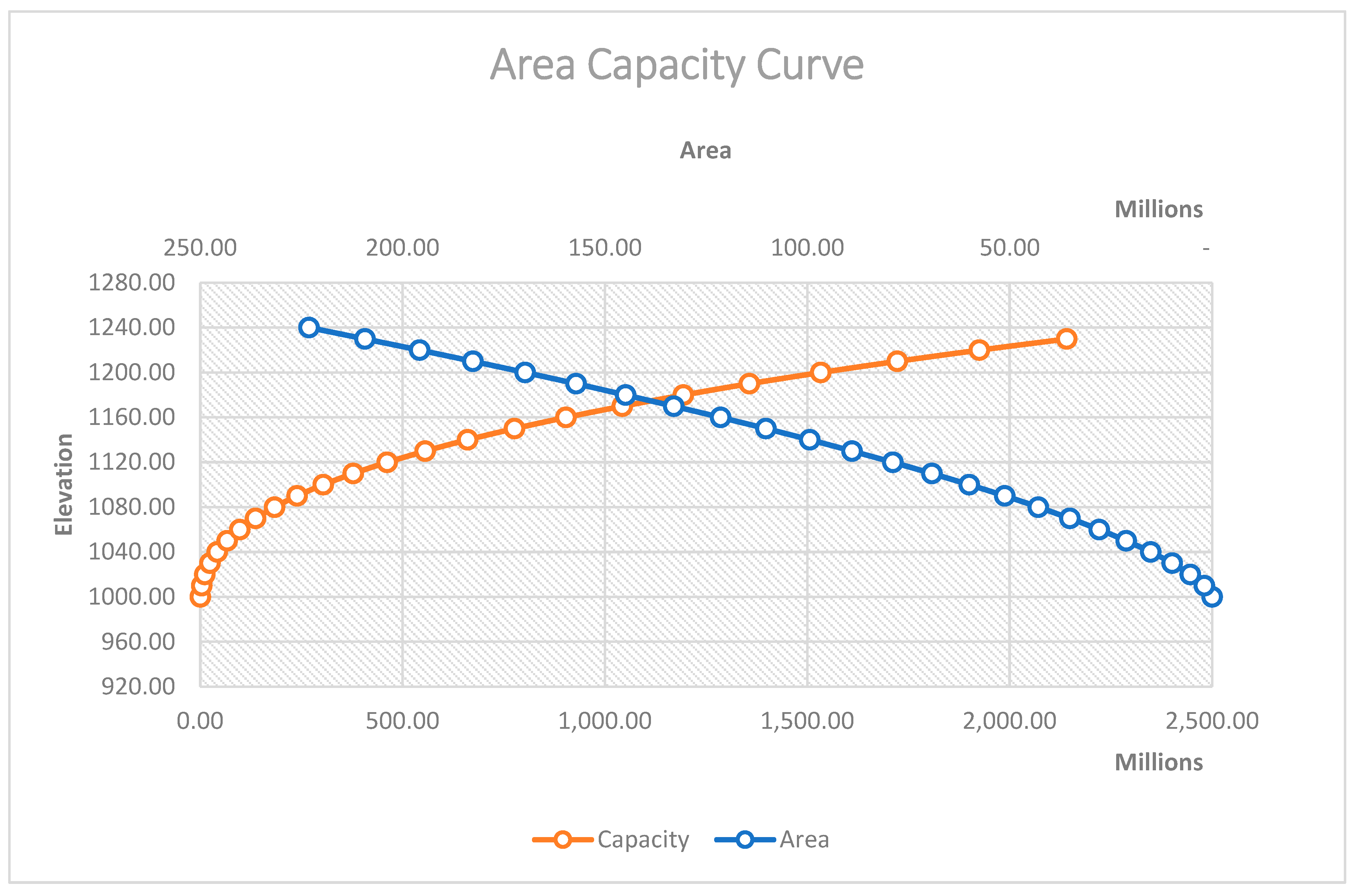
Figure 4-2.
Flow duration curve.
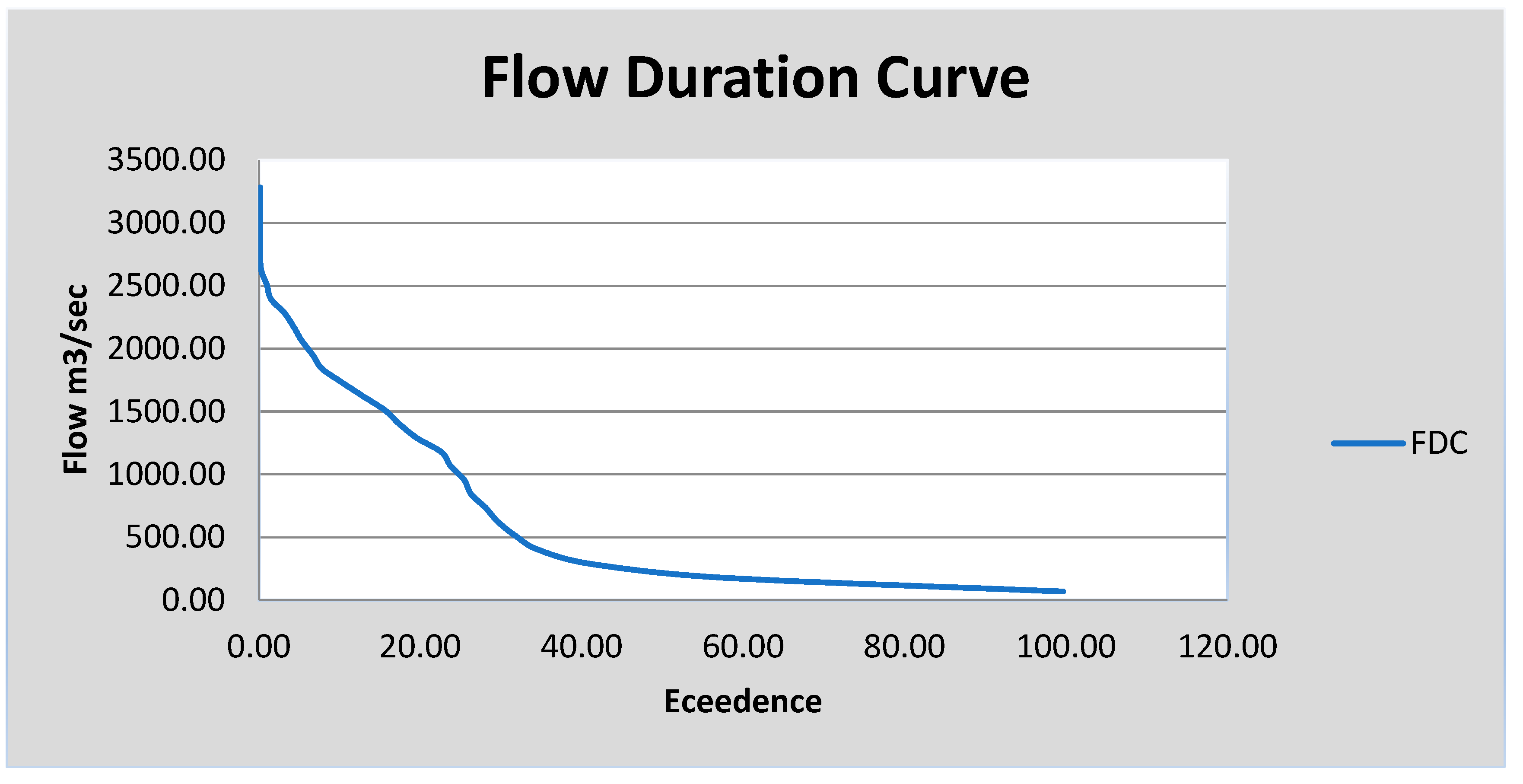
Table 3-1.
Comparison of estimation methods based on RMSE, MAE and R with 20% missing value for stream flow data.
Table 3-1.
Comparison of estimation methods based on RMSE, MAE and R with 20% missing value for stream flow data.
| Station | Method | RMSE | MAR | R |
| 20% | ||||
| G | AA | 176 | 75 | 8.0 |
| ID | 150 | 72 | 7.8 | |
| NR | 155 | 73 | 7.9 | |
| CC | 154 | 73 | 7.7 | |
| I | AA | 170 | 76 | 7.9 |
| ID | 146 | 71 | 8.2 | |
| NR | 152 | 72 | 7.7 | |
| CC | 150 | 74 | 7.6 | |
| J | AA | 171 | 76 | 7.9 |
| ID | 151 | 71 | 7.8 | |
| NR | 158 | 73 | 8.1 | |
| CC | 152 | 74 | 7.83 | |
| N | AA | 166 | 75 | 7.9 |
| ID | 159 | 71 | 8 | |
| NR | 150 | 73 | 7.7 | |
| CC | 155 | 73 | 7.6 | |
Table 3-2.
Comparison of estimation methods based on RMSE, MAE and R with four different percentages of missing values for stream flow data.
Table 3-2.
Comparison of estimation methods based on RMSE, MAE and R with four different percentages of missing values for stream flow data.
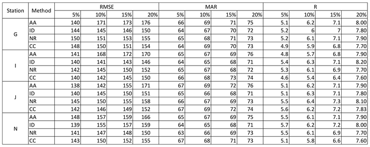 |
Table 5-9.
Adjusted Domestic Water Demand for H project Town.
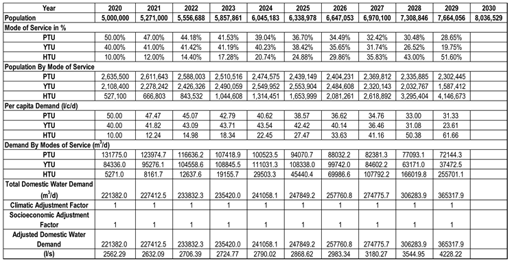 |
Table 4-1.
Crop water and irrigation requirement of different crops (m3/ha).
| Crop | Planting Date | Growing period (days) | Seasonal Etc/m3/ha | Irrigation req/m3/ha |
|---|---|---|---|---|
| Onion | 01-Feb | 95 | 4624 | 4226 |
| Tomato | 01-Jan | 145 | 7421 | 6649 |
| Wheat | 15-Jan | 130 | 6083 | 5445 |
Table 4-3.
Q95 for downstream release.
| Q70 | Q80 | Q95 |
|---|---|---|
| 147.49 | 121.49 | 82.50 |
| Monthly Volumetric water requirements for downstream release in m3 Q95 | 213,839,358.75 | |
Disclaimer/Publisher’s Note: The statements, opinions and data contained in all publications are solely those of the individual author(s) and contributor(s) and not of MDPI and/or the editor(s). MDPI and/or the editor(s) disclaim responsibility for any injury to people or property resulting from any ideas, methods, instructions or products referred to in the content. |
© 2023 by the authors. Licensee MDPI, Basel, Switzerland. This article is an open access article distributed under the terms and conditions of the Creative Commons Attribution (CC BY) license (http://creativecommons.org/licenses/by/4.0/).
Copyright: This open access article is published under a Creative Commons CC BY 4.0 license, which permit the free download, distribution, and reuse, provided that the author and preprint are cited in any reuse.


