Submitted:
25 November 2023
Posted:
27 November 2023
You are already at the latest version
Abstract
Quaternion algebra is used both for the description of the motion of material objects in 4D space-time and for the representation of the energy-momentum density tensor in the same quaternion basis, accurate to some arbitrary scalar fields. Quaternionic generating operators applied repeatedly to the energy-momentum density tensor lead to the gravitomagnetic equations that are parent equations for the series of physical equations ranging from the wave equations up to the quantum mechanical ones. Before finally deducing the gravitomagnetic equations, it is necessary to use the Lorentz gauge at a certain stage to cut off the arbitrary scalar fields. We declare that these superfluous scalar fields, inaccessible to direct observation, represent dark matter and dark energy. We show in what way the dark matter can provide a flat profile of the orbital speed of the galaxy's arm rotations.
Keywords:
Navier-Stokes equation
; vorticity equation
; toroidal vortex
; irrotational velocity
; solenoidal velocity
; spiral galaxies
; dark matter
; dark energy
1. Introduction
The cosmological principle states that the spatial distribution of matter in the universe is homogeneous and isotropic when viewed on a sufficiently large scale. In this view, let us first evaluate the mass density of the visible universe. With its diameter d equal to about 28.5 gigaparsecs [1], or , its volume is as follows . Hereafter we will adhere to SI units. The total mass of visible matter in the universe according to different sources [2,3,4] is about to kg. We take the average kg. From here we may evaluate the mass density of the visible matter filling the visible universe
Planck Collaboration [5], Planck Collaboration [6], Planck Collaboration [7] has shown from the measurements of the CMB anisotropies a good consistency with the standard spatially flat 6-parameter CDM cosmology. It follows from here that one can take Euclidean flat geometry, where the average density is close to the critical density [8,9]:
Here is the gravitational constant. The Hubble constant expressed in units adopted in astrophysics [10] is about . Or it is being represented in SI unit [11]. Now, we can estimate the presence of visible matter and the matter composing the critical density (dark matter and energy) in the observed universe as a percentage
So, the visible (baryon) matter is only about in the visible universe. The remaining are the dark mass and dark energy. It is exactly what our instruments do not detect, except that the dark matter has gravity.
There is a reason to believe that the dark matter and dark energy are basically Bose-Einstein condensates [8,12,13,14,15,16,17] representing the superfluid quantum medium [18,19,20,21]. We call it as the superfluid quantum space-time [22,23], since this medium fills all the space everywhere densely, being the physical vacuum. Albareti et al. [24,25] consider that the large-scale structure of physical vacuum may manifest very much in the same way as cold dark matter does. One can notice that the above medium is an updated version of the ether, which was unfairly rejected but then accepted again, thanks in particular to the authorities of Einstein [26] and Dirac [27].
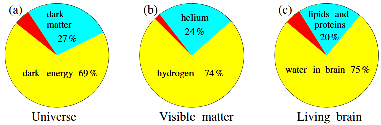
Qualitatively, the distribution of matter in the universe can be represented in pie charts, as shown in Figure 1.
The first pie chart (a) in Figure 1 shows the presence of dark energy, dark matter, and visible matter that make up the universe. It can be seen that, against the background of dark energy and dark matter, visible matter is only a small part. Figuratively speaking, if dark matter and energy are the bulk of the boundless ocean, then visible matter appears to be a fleeting foam on it.
The following pie chart (b) shown in Figure 1 demonstrates the presence of various atomic elements within this fleeting baryon foam. It can be seen that these elements are mainly hydrogen and helium. Only hydrogen, the carrier of protons, and helium, the carrier of both protons and neutrons, account for up to 98% of all visible matter, which washes the entire universe in a thin layer. The remaining two percent of visible matter is accounted for by all other atoms heavier than helium.
As for the third diagram represented in Figure 1, it shows what chemical and biochemical components the living brain consists of. This group includes such elements as sodium, potassium, nitrogen, carbon, calcium, oxygen, iron, zinc, selenium, magnesium, and other higher elements that are the basis of living matter. As seen, the organization of the living brain needs many chemicals, which are a tiny percentage of visible matter. It means that living, intelligent matter is an exceptionally rare phenomenon in the universe. But it is this intelligent matter that realizes the greatness of the universe.
The article is organized as follows: In Sec. 2 we apply the quaternion generating operators to the energy-momentum tensor written on the same quaternion basis. Note that the energy-momentum tensor is defined up to two scalar fields. One scalar field, the massless field, relates to the EM field. The other field, the mass-loaded field, deals with the mechanical part of the tensor. To arrive at the gravitomagnetic equations, we should accept the Lorentz gauge as cutting off these scalar fields. Our attention here is on the invisible world that arises due to applying the Lorentz gauge. We declare in sec. 3 that these scalar fields deal with dark energy and dark matter. The manifestation of dark matter will be confirmed by its contribution to the stabilization of the rotational velocities of spiral galaxy arms. With that aim in mind, we first derive, in sec. 4, the gravitmagnetic equations. Further, we get the Navier-Stoces equation in sec. 5, and next we obtain the vorticity equation and its solutions for the orbital speed, subsets. 5.1 and 5.2. The result is a flat profile of orbital speed stabilized by applied dark matter chunks. Concluding remarks are given in sec. 6.
2. Quaternion Framework of the Space-Time Continuum
In mathematics, quaternions are a commutative number system that extend complex numbers. Quaternions were first described in print by Linda Rodriguez about in 1840 and independently discovered by the Irish mathematician Sir William Rowan Hamilton [28] in 1843 and applied to mechanics in three-dimensional space. Here is what James Clerk Maxwell [29], the discoverer of electromagnetic theory, wrote about the discovery of the quaternion calculus: “The invention of the calculus of quaternions is a step towards the knowledge of quantities related to space which can only be compared, for its importance, with the invention of triple coordinates by Descartes. The ideas of this calculus, as distinguished from its operations and symbols, are fitted to be of the greatest use in all parts of science.” There is, however, an amazing compatibility between the coordinate framework of 4D spacetime and the quaternions, () described by William Rowan Hamilton. Nevertheless, instead of these numbers, further we introduce the quaternion basis represented by four matrices with real-valued components [23,30,31,32,33,34,35,36,37,38]:
These four -matrices, , , , , are isomorphic to four matrices , , , [39,40,41,42,43,44]. The latter matrices belonging to the group SU(2) are the main elements used by Roger Penrose at formulations of his twistor theory [45,46,47,48].
The matrices , , , obey the following multiplication rules:
All mathematical relations of the quaternion group can be obtained from these algebraic equations. Note that the orders of multiplication and are opposite to each other. This chirality violation was introduced when studying the passage of polarized neutrons through magnetic fields [30], since the correspondence of the direction of the magnetic field and the spin of the neutron was observed. The recovery of symmetry is achievable by changing the sign at any matrix , , or .
Let us now define the generating differential operators [23,35,36,37,49], as follows:
which are needed for reproducing the space-time dynamics of a medium described by the energy-momentum density. In particular, the D’Alembert wave operator for the case of the negative metric signature reads
Now let us turn to the consideration of the medium evolving in this 4D space-time. We begin with terms and representing the kinetic energy and momentum of matter enveloped by the electromagnetic potentials and :
Here is the Lorentz factor. At the non-relativistic limit, , it tends to the unit. The density in these equations multiplied by m or by e (mass and charge of the unit carrier – particle) returns the mass density and the charge density , respectively. Here and are the rough mass and charge of the material body containing N particles within the elementary volume under consideration. Note that the particles within this volume make chaotic walks, obeying the uncertainty principle at collisions [50,51]. In the first approximation, these walks permit description by the Wiener process [52,53]. As a result, a blurred cloud of the particles arising permits us to describe their evolution by a wave function.
Now, we introduce two gauge invariant scalar fields [36]. One scalar field, , relates to the massless electromagnetic medium loaded by the electromagnetic potentials and . Carriers here are EM quanta with zero rest mass. The other scalar field, , deals with the mass loaded medium which has the kinetic energy and momentum describing a state of this medium. The other scalar field, , deals with the mass-loaded medium. It has the kinetic energy and momentum describing the state of this medium. Let us rewrite Eq. (9) in light of the above said
The energy-momentum tensor written in the quaternion basis looks as follows
Here and are the generalized energy and momentum densities (9) and is an arbitrary scalar field, having dimensionality of . Observe that, has the same dimension, applied by Fedi [54] for the explanation of the ether being the Newtonian fluid manifesting this effect at the relativistic speeds.
Let us now apply the generating operator to the energy-momentum tensor (11):
We proclaim that the multiplier of the unit quaternion returns the Lorentz gauge, namely:
So that only the expressions of the quaternions , , remain, which do not contain terms with . As a result, we may rewrite equation (12) in the following manner
This form is the gravitomagnetic tensor represented in the quaternion basis.
In the quaternion basis the electromagnetic tensor has the same form [42]. It is instructive to compare this electromagnetic tensor represented in the quaternion basis with a tensor written in the usual form in the theory of electromagnetism
The complex gravitomagnetic field in Eq. (14), as follows from computations in Eq. (12), reads:
Here and are electric and magnetic fields. By analogy, and are gravitational and torsion fields. But more definitely, they determine irrotational and solenoidal fields. We will raise this topic further when we discuss Helmholtz’s theorems relating to such flows.
3. The Arbitrary Scalar Field Represents a Dark Energy Ocean
Let us study the arbitrary scalar field in more detail. We rewrite Eq. (13):
Here and . The scalar product of the 4-gradient operator by the 4-vector defines the 4-divergence . Thus, it is a 4D divergence of the energy-momentum of our world acting on the invisible world. Let us evaluate the scalar field represented in Eq. (17). Note first that since has the dimension J·m−3 then the term has the dimension J·m−4. From here it follows that has the dimension J·m−2 = kg·s−2. The scalar field as this estimation indirectly indicates, relates to the physical vacuum that behaves as a non-Newtonian (dilatant) fluid as shear stress increases [54,55]. This means that the fluid viscosity grows with the increasing material body velocity moving through the fluid (it is equivalent to its inert mass growing). The fluid "hardens" with increasing shear stress.
The scalar field relates to the massless electromagnetic field. While deals with the gravitomagnetic field loaded by mass. If so, then let us rewrite the first term and in Eq. (17) as follows:
We declare that the part covered by brace (a) vanishes:
The first equation covered by brace (a0) is the Klein-Gordon equation that obeys the "on-shell condition" [38]. Further, we rewrite this equation by extracting two Dirac operators multiplied by each other, as shown in the bracket (a1). Here, the multiplication of these operators yields the sum . Note that , where is the Minkowski metric with signature and . Thus, vanishes.
This means that the multiplication of two Dirac operators under brace (a1) describes the action of a coupled pair of particle and antiparticle, each with a half-integer spin. It is a boson with an integer spin. Its behavior is described by the Klein-Gordon equation. This equation states that (a) both fermions rotate about the common mass center; (b) the bonded fermions have zero charge; (c) the bonded fermions have integer spin equal to either 0 or ±1; (d) and they have equal masses, Figure 2. There are possible spontaneous transitions from bound fermions to massive scalar waves described by the following equation:
and vice versa. The mass shell is a hyperboloid in the energy-momentum space, which is described by solving the following equation:
This formula states that the energy and momentum of the particle and antiparticle are interconnected through the Einstein relation, and they lie on the mass surface.
Let’s return to Eq. (18). A hidden term covered by bracket (b) can be accepted as the dark matter manifestation. From the computations made above, these unknown particles are bosons composed of coupled pairs of particles and antiparticles. Following Occam’s Razor principle, we will not invent exotic particles but focus on baryon particles, like widespread atomic hydrogen [56,57]. Such a Bose-Einstein condensate of baryon-antibaryon matter exists at a temperature of T = 2.75 K. It is the cold dark matter [14,21,24,25]. Because of the Meissner effect, it is not visible by EM radiation.
Evaluations say that the critical density, , can be achieved if 18 proton masses are contained within the volume of m3, namely, , compare with Eq. (2). For the visible matter, only one proton mass is in the volume, about m3. We find , compare with Eq. (1).
Eighteen invisible proton masses versus one visible proton mass are seen to define a general picture of the gravitational influence of dark matter on visible baryon matter. The problem is to define the mechanism leading to the mechanism of vortex capture by invisible matter, visible as they rotate around a common center. Surprisingly, such a capture mechanism was experimentally studied by [58,59] in terrestrial laboratory conditions. Further, we will consider such a capture mechanism. But before that, we need to get the vorticity equation that describes a vortex exchanging with the quantum ether through viscosity fluctuations.
4. Equations of the Real Gravitomagnetic Field
Let us now return to the end of Sect. 2, to Eq, (14). Our aim here is to obtain the vorticity equation and to show how dark matter influences the rotation of vortex tails.
First, we note that the gravitomagnetic fields stem from the force density tensor, , after applying the transposed generating differential operator [36,38]. For this reason, first we define a 4D current of the force density that takes into account gravitation influence, electromagnetic, and other accompanying forces acting on the medium within the volume under consideration. We define the density distribution term of all forces acting on the medium enclosed within this unit volume as follows:
The divisor is introduced to emphasize the commonality with Maxwell’s EM equations. Here considers external forces acting on the medium inside the volume and its internal reaction on these forces with pressure gradients arising in this medium [42]. In addition, we must consider the shear viscosity due to friction of the medium layers induced by the pressure gradients. We could omit this effect from our consideration in the first approximation. Note, however, that because of this neglect, we can face unwanted singularities in subsequent calculations. The following step defines the 3D current density as . Here is the velocity of the unit volume of the medium in question. Finally, we define the 4D current density as follows:
The continuity equation for this current is
This is a manifestation of Newton’s third law.
By applying the transposed generating differential operator to the force density tensor (14) and equating it to the 4D current density we come a set of gravitomagnetic equations:
One can see first that here we get the wave equation for the energy-momentum density tensor subjected to the external action of 4D density current . Amazing complementarity takes place between Eqs. (13) and (25) if we use the term accepted in Eq. (23). Note that Eq. (25) describes wave oscillations of the visible matter, while Eq. (13) does the same with the invisible matter and energy.
Now revealing in detail the product we obtain the following expanded equation, where its terms have been sorted as coefficients under the quaternions , , , :
On the left side of this equation, braces enveloping terms equal those being represented on the right side when their real and imaginary values permit it. Otherwise, they are zero. By gathering real and imaginary parts at the quaternions , , , , we obtain the gravitomagnetic equations
As noted above, the gravitomagnetic fields are represented by the superposition of the gravitotorsion fields and the electromagnetic fields . It can be noted here that these equations are ancestral equations leading to sets of wave equations, vorticity equations, and Hamilton-Jacobi equations describing the motion of material bodies in ideal and viscous media, as well as the quantum mechanical equations [23,34,36,37,42,60,61,62,63]. Here, we omit this detailed analysis. Instead, we will immediately proceed to the last part - the analysis of the Navier-Stokes equation, opening a path to the vorticity equations.
The problem here is to determine parameters that can lead to the appearance of a flat orbital velocity profile. Looking ahead, it can be noted that the critical parameter in this matter may be the viscosity of the medium. Since the medium is a superfluid with zero viscosity, the viscosity dispersion around zero can be such a critical parameter.
5. Navier-Stokes Equation: Forward to the Vorticity Equation
Let us look on Eq. (28). By rewriting the expression in details we have
The term is an arbitrary solenoid force density. It disappears when the gradient operator is applied to this equation. Here, the force density comes from Eq. (22). It is the sum of all force densities acting on the medium under consideration within a unit volume. They are (a) external forces; (b) internal forces represented by the pressure gradients arising in the medium under the action of the external forces; and (c) forces leading to the sliding of the layers of the medium on each other (they can lead to heat losses).
Considering the above, we get the equation for incompressible fluids, [64], divided preliminarily by the density distribution :
This is the modified Navier-Stokes equation. Here and we have (a) the external force is conservative and can be represented as a negative gradient of the external potential energy U, and (b) the pressure gradient can be rewritten by adding an extra term, i.e., the pressure multiplied by the gradient of logarithm from the density distribution. As a result, it leads to a gradient of the quantum potential Q. In this equation, we represent the external potential and the quantum potential as the sum under the gradient. And (c) the viscosity coefficient is due to the layers sliding because of the pressure gradient arising within the medium.
It would seem that if the medium is superfluid, then the viscous term can be zeroed out in the first approximation. However, as practice has shown, sooner or later, when analyzing such an equation, you will have to face singularities. To get around these obstacles, a scientist usually shifts the poles of a Green function to the negative real half-plane. In fact, he manually enters the attenuation. We will not reject viscosity. However, we believe that the average viscosity vanishes over time, but its variance is not zero.
The term is the kinematic viscosity coefficient. Its dimension is [m2s−1] such as that of the diffusion coefficient. However, the medium, which fills all spaces densely, is superfluid [18,20,65,66]. Therefore, such a medium is considered to have a zero viscosity coefficient, . However, as was said above we assume that the viscosity, adhesion, of the medium is zero on average over time, but its dispersion is not zero [36,42,60,67]:
These expressions describe an exchange of energy with the superfluid ether medium, the invisible world, as described in Sec. 3. The first relation states that, on average, there is no exchange with the invisible world in time. From the second expression, it follows that the exchange occurs regularly, both with the return of energy and with its acquisition randomly. It should be noted that since the viscosity coefficient depends on time but does not contain spatial variables, the invisible medium is non-local and consists of the Bose-Einstein condensates.
Before considering the vorticity equation, we apply the Helmholtz decomposition theorem of velocity into two components, irrotational velocity and solenoidal velocity:
where subscripts I and O indicate the existence of irrotational and orbital (solenoidal, rotational, tangential) fluid velocities. We write the subscript O (orbital) instead of S (solenoidal) because the letter S relates to the notation of the scalar field and the action function S.
The component irrotational, , and orbital, , velocities satisfy the following conditions:
Now, let us apply the curl operator to Eq. (32). We obtain [61]
Here is a vorticity resulting from applying the curl operator to the arbitrary external solenoidal force . For simplicity, we consider it equal to zero. The term covered by brace (a) describes the dissipation of energy stored in the vortex.
Figure 3.
The vortex shown in the cylindrical coordinate system extends from minus infinity to plus infinity [36]. The vortex wall is a boundary where the orbital speed, , reaches maximal values; a is the radius of the vortex tube, is the vorticity. Profiles of the orbital velocity at different N [36]: (a) , normal profile of the Lamb-Oseen vortex orbital velocity [68]); (b) , profile of the non-decreasing solenoidal velocity with distance as for rotating spiral galaxies, for example [69].
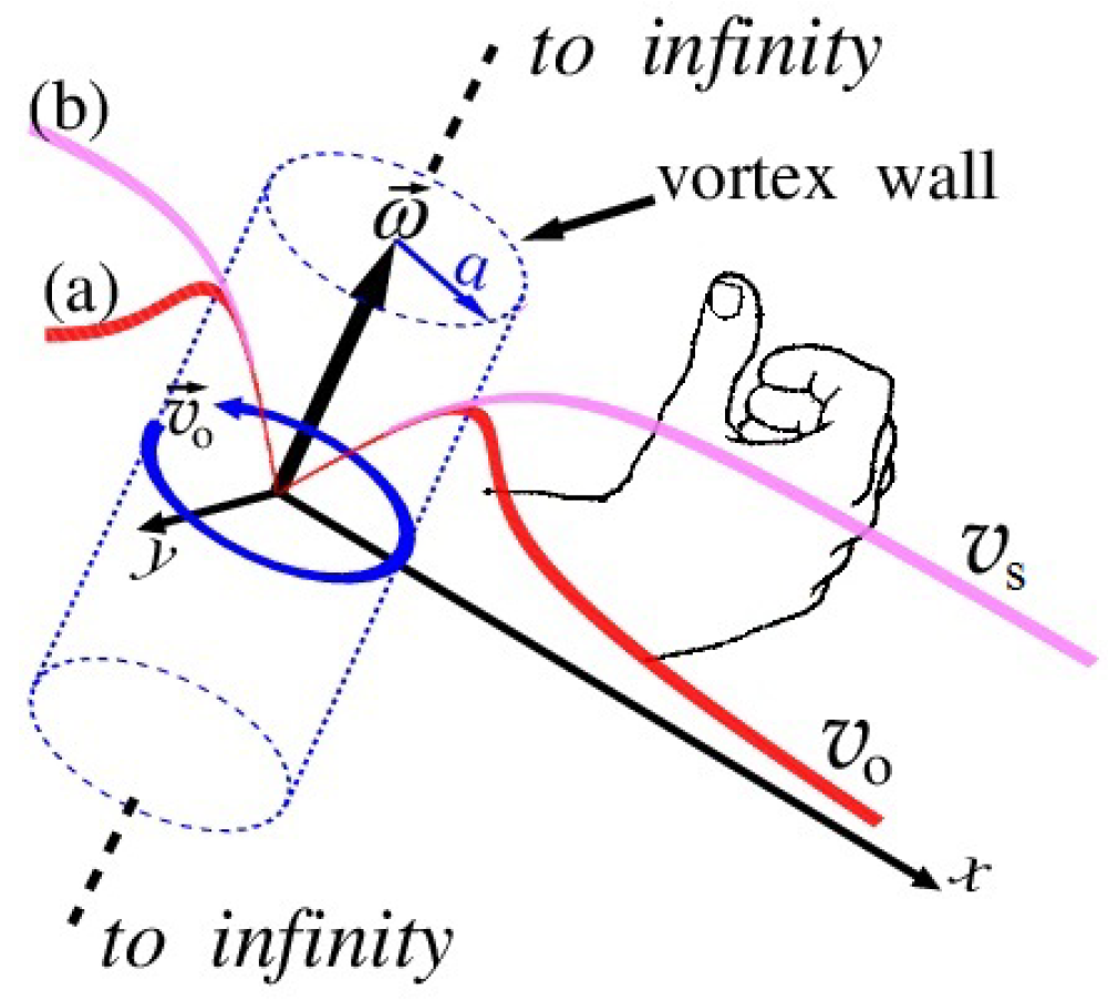
By omitting this term (i.e., assuming ), we proceed to the action of the Helmholtz theorem [70]: (i) if fluid particles form, in any moment of time, a vortex line, then the same particles support the vortex line both in the past and in the future; (ii) ensemble of the vortex lines traced through a closed contour forms a vortex tube; (iii) intensity of the vortex tube is constant along its length and does not change in time. The vortex tube drawn in Figure 3 either (a) goes to infinity by both endings; or (b) these endings lean on boundary walls containing the fluid; or (c) these endings are locked to each other, forming a vortex ring.
Now we will not remove the viscosity. Instead, we hypothesize that the viscosity fluctuates around zero. Its expectation is zero. These fluctuations represent the exchange of stored energy in the vortex with zero-point vacuum oscillations. Since , the vortex does not completely disappear. It is a long-lived object.
Here, we consider a redial component of the vortex dynamics. Let us look at the vortex tube in its cross-section, which is oriented along the z-axis and its center is placed in the origin of the plane , Figure 3. Eq. (36), written in this cross-section, appears as follows:
A general solution to this equation has the following view of vorticity [36]:
and orbital speed
Here is the integration constant having dimension [length2/time]. And the denominator looks as
Here is an integration constant. It is such that the denominator must be positive regardless of how the viscosity coefficient fluctuates, whether the fluctuations look like white noise, or whether they contain periodic components.
5.1. Lamb-Oseen Vortex, Pancake Vortex, and Rogue Wave
Note that for viscous hydrodynamic flows (), the above formulas with simulate a decaying line vortex because of nonzero viscosity
At this solution is that of the Lamb-Oseen vortex [68]. A normal profile of the orbital velocity of the Lamb-Oseen vortex rotating about the central axis of the vortex tube is shown in Figure 4a. One can see that the velocity grows from the central axis up to the vortex wall. Next, it sharply decreases as one moves away from the origin. At the orbital velocity also grows from the central axis up to the vortex wall. But next, it begins monotonically to decrease the slower, the larger , as the distance terns to infinity, Figure 4b. This indicates the path of the search for the flattening of the orbital velocity profile in the region far from the origin.
When we reject in Eqs. (41) and (42) these solutions degenerate into the so-called long-lived Gaussian pancake vortices [71,72,73]. Note that such long-lived Gaussian pancake formations arise because of the inserted parameter as an arbitrary integration constant, which was not originally provided in the equation (36). We had to introduce this parameter to prevent singularities that may occur due to fluctuations in the viscosity coefficient.
There are phenomena observed in ocean hydrodynamics that show pancake vortex formations. These are killer waves (wandering waves, monster waves, white waves, rogue waves, freak waves, crazy wave) – giant single waves [74,75] arising in the ocean, 20–30 meters high (and sometimes larger), having uncharacteristic behavior for sea waves. An important circumstance is the suddenness of their appearance and disappearance. We can hypothesize that the appearance and disappearance of killer waves are caused by fluctuations of clumps of dark matter, which induce giant wandering waves on the expanses of movable ocean water. Note that the mass of dark matter is five times greater than that of visible matter. Ancient civilizations may have learned about this phenomenon by erecting monumental structures such as pyramids.
5.2. Rotation of Spiral Galactic Arms
Let us return to Eqs. (38)-(40). Because the viscosity coefficient fluctuates about zero according to our assumption, Eq. (33), the integral in Eq. (40) returns zero. For that reason the solution written in Eq. (39) takes an exceptionally simple form
The coherent Gaussian vortices, being time-independent objects, allow superposition:
where grows with increasing n. For simplicity, we consider the following simple dependence:
Figure 3 shows the orbital speed as a function of the distance r for two different cases: , and , respectively. The profile of the speed grows monotonically as r increases from the center of rotation. In the case of , the speed after reaching the vortex wall begins to drop monotonously, Figure 3, curve (a). For a sufficiently large N, the speed behind the vortex wall comes to a flat level, Figure 3, curve (b). This case agrees well with the astronomical observations of the orbital speeds of rotating spiral galaxies [76]. Figure 5 shows the orbital speeds for different N as functions of time.
The fact that time is not explicitly represented in the formulas (43)-(44) is because fluctuations of the viscosity coefficient, , are defined as the white noise (33). In principle, we can define the existence of some harmonic oscillations [77] against white noise, which simulate the breathing of a galaxy. Figure 6 shows such an imitation of breathing. It is visible as ripples of the flat plateau on the curve.
This breathing is caused by the exchange of energy with the physical vacuum at ultra-low frequencies owing to the term . At these ultra-low frequencies, this exchange occurs via virtual particle-antiparticle pairs, i.e., proton-antiproton pairs, as stated above. This manifestation stems from dark matter [69]. The ultra-low frequencies are perhaps due to the slow shifting of the dark matter clumps as the galaxy evolves further. Such a shifting of the dark matter one can guess is a consequence of the galaxy evolution processes.
As follows from numerous observations, the flat profile of orbital velocities during the rotation of spiral galaxies around their central core can be provided by additional invisible matter, called dark matter [69,78]. De Blok et al. [76] have presented a rich set of rotation curves, Figure 7, supporting the tendency of the orbital velocities of rotating galaxy arms to possess a flat profile. Thirty diagrams showing the orbital velocity (km·s−1) versus the distance r (in kiloparsec) demonstrate different profiles, where do not always follow up well with the monotonous outlet of curves on to a flat profile.
Sbitnev and Fedi [11] have approximated these curves using the formulas given in Eqs. (43)-(45). Only instead of we have assigned being fitted for each individually. The task was to draw the curve passing within confidence intervals so that it came to experimentally measured points as closely as possible. Fitted curves are drawn in red in Figure 7 against the black-white data [76] representing the orbital speed of galaxies measured by [72]. These curves fit the confidence intervals quite well. However, an important remark according to this fitting is that the fitting coefficients for low have a large scatter. This indicates that the blocks of dark matter are not ordered but rather chaotically organized. It appears that the observed galaxies are in a transitional stage of evolution. Most likely, there is a dynamic evolution occurring here - a change in the motion of the components of the galaxy (in this case, clumps of dark matter, perhaps, together with visible matter as well).
6. Conclusion
Quaternions written out as four matrices of rank 4x4 are natural variables describing the algebra of the 4D spacetime having 10 degrees of motion freedom. Within the framework of the quaternion basis superimposed on 4D space-time, the energy-momentum density tensor is recorded, which describes the current state of visible matter in this 4D space-time. Note that the density tensor consists of the superposition of two parts. The first part describes the mechanic-rotational state of the visible matter, loaded by brute mass. The second part deals with the electromagnetic state of this matter, loaded by distributed charges. By applying differential generating operators to this energy-momentum density tensor, we disclose a whole set of equations describing the behavior of our visible world.
One point that the author has tried to avoid until now concerns an unclear description of the energy-momentum density tensor. In principle, it can be determined up to an arbitrary scalar field, which subsequently does not affect the results of calculations in any way. Cutting off this scalar field is achieved by imposing a Lorentz gauge condition. After performing that operation, you can forget about the existence of such a scalar field.
Observe, however, that the Lorentz gauge represents the Klein-Gordon equation for this arbitrary scalar field, where the right part is represented by partial derivatives of the energy-momentum density tensor. While the left part contains two scalar fields subjected to the action of the D’Alembert wave operator. These two scalar fields relate to the mechanical-rotational and electromagnetic energy-momentum density tensors. The first scalar field is a mass-loaded one. We can add and subtract a certain mass-carrying term and thereby derive the Klein-Gordon equation loaded with mass in explicit form. This equation describes the coexistence of particles and antiparticles on a mass shell. The second scalar field relating to the electromagnetic field is mass-free. This gives rise to the following assumption: that the Lorentz gauge offers a description of the invisible world, represented by dark matter and dark energy. In fact, this invisible world is the superfluid quantum ether that many scientists write about.
The interaction of this ether with our visible world is possible due to the fluctuation of viscosity, which is zero on average over time. Note, first, that solutions of the vorticity equation contain both the viscosity coefficient multiplied by time and a vague integration parameter having the dimension [meter2]. Usually, this parameter is discarded as unnecessary. The remaining solution is known as the Lamb-Oseen vortex, which rapidly relaxes to zero as time and distance go on. However, the integration parameter turns out to be decisive in describing the so-called long-lived Gaussian pancake formations, which represent dangerous rogue waves in the ocean. If under terrestrial conditions the lifetime of such killer waves is limited to the coastlines of continents, then in the gaseous atmosphere of Jupiter their lifetime can be unlimited. An important point for us is not only the extension of the lifetime of such Gaussian pancake formations, but also the flattening of their profiles with distance.
We argue that the inclusion of this vague integration parameter in the vortex solution is necessary to prevent the appearance of singular jumps that could arise due to fluctuations in the viscosity of the medium. The emergence of this vague integration parameter is due to the dark matter chunks exchanging energy fluctuations with the visible matter through the viscosity fluctuations
Because of the fluctuation in viscosity, chunks of dark matter pull visible matter behind them. Can it be observed in terrestrial experimental conditions? Perhaps a similar pulling up of a non-rotated driven disk by the drive disk has been observed by Prof. Samokhvalov [79]. The author, having studied the works of Samokhvalov, proposed to investigate the effect of this unknown force, pulling an unstoppable, driven disk, with the involvement of neutron interferometry [36].
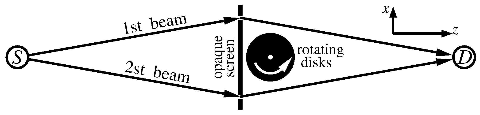
The meaning of neutron interferometry is to repeat the Aharonov-Bohm experiment [80] to register the effect of the electromagnetic vector potential "immured" in a cylinder shielding magnetic fields. The diagram of the neutron interference experiment is shown in Figure 8. It is expected that if the capture of a stationary slave disk is caused by the reorganization of clumps of dark matter, the measurement result will show the appearance of asymmetry in interference fringes.
Funding
This research received no external funding.
Acknowledgments
It was planned to complete this manuscript with a chapter titled “The Interaction of Consciousness with the Invisible World”, written in co-authorship with Prof. Dirk K. F. Meijer. However, because of the weak verifiability of that scientific issue, this chapter was rejected. But we hope that the problem of the interaction of consciousness with the invisible world will eventually be raised in the open press.
Conflicts of Interest
The author declares no conflict of interest.
References
- Bars, I.; Terning, J. Extra Dimensions in Space and Time; Springer: New York, Dordrecht, Heidelberg, London, 2010. [Google Scholar] [CrossRef]
- Immerman, N. The Universe. WebSite 2001. http://www.cs.umass.edu/ immerman/stanford/universe.html.
- Davies, P. The goldilocks enigma; A mariner book, Houghton Mifflin Co.: Boston, N. Y., 2006.
- Vlahovic, B. A New Cosmological Model for the Visible Universe and its Implications. Preprint-arXiv 2011, 1005.4387. [CrossRef]
- Planck Collaboration. Planck 2013 results. I. Overview of products and scientific results. Astronomy & Astrophysics 2014, 517, 1–48. [Google Scholar] [CrossRef]
- Planck Collaboration. Planck 2015 results. XIII. Cosmological parameters. Astronomy & Astrophysics 2016, 594, 1–63. [Google Scholar] [CrossRef]
- Planck Collaboration. Planck 2018 results VI. Cosmological parameters. Astronomy & Astrophysics 2020, 641, 67. [Google Scholar] [CrossRef]
- Nishiyama, M.; Morita, M.; Morikawa, M. Bose Einstein Condensation as Dark Energy and Dark Matter. arXiv, 2004; astro-ph/0403571. [Google Scholar] [CrossRef]
- Ryden, B. Introduction to Cosmology; The Ohio State University, 2006.
- Freedman, W.L.; Madore, B.F.; Gibson, B.K.; Ferrarese, L.; Kelson, D.D.; Sakai, S.; Mould, J.R.; Kennicutt, Jr., R.C.; Ford, H.C.; Graham, J.A.; Huchra, J.P.; Hughes, S.M.G.; Illingworth, G.D.; Macri, L.M.; Stetson, P.B. Final Results from the Hubble Space Telescope Key Project to Measure the Hubble Constant. Astrophys. J. 2001, 553, 47–72. [CrossRef]
- Sbitnev, V.I.; Fedi, M. Superfluid Quantum Space and Evolution of the Universe. In Trends in Modern Cosmology; A. J. Capistrano de Souza., Ed.; InTech: Rijeka, 2017; chapter 5, pp. 89–112. [CrossRef]
- Boehmer, C.G.; Harko, T. Can dark matter be a Bose-Einstein condensate? JCAP 2007, 2007, 025. [Google Scholar] [CrossRef]
- Harko, T.; Mocanu, G. Cosmological evolution of finite temperature Bose-Einstein Condensate dark matter. Phys. Rev. D 2012, 85, 084012. [Google Scholar] [CrossRef]
- Bettoni, D.; Colombo, M.; Liberati, S. Dark matter as a Bose-Einstein Condensate: the relativistic non-minimally coupled case. JCAP 2014, 2014, 004. [Google Scholar] [CrossRef]
- Dwornik, M.; Keresztes, Z.; Gergely, L.Á. Rotation curves in Bose-Einstein Condensate Dark Matter Halos. In Recent Development in Dark Matter Research; N. Kinjo, A.N., Ed.; Nova Science Publishers: N.Y. USA, 2014; chapter 6, pp. 195–219.
- Das, S.; Bhaduri, R.K. Dark matter and dark energy from Bose-Einstein condensate. Class. Quant. Grav. 2015, 32, 105003 (6 pp). [Google Scholar] [CrossRef]
- Sarkar, S.; Vaz, C.; Wijewardhana, L.C.R. Gravitationally bound Bose condensates with rotation. Phys. Rev. D 2018, 97, 103022. [Google Scholar] [CrossRef]
- Sinha, K.P.; Sivaram, C.; Sudarshan, E.C.G. Aether as a Superfluid State of Particle-Antiparticle Pairs. Found. Phys. 1976, 6, 65–70. [Google Scholar] [CrossRef]
- Vigier, J.P. Alternative interpretation of the cosmological redshift in terms of vacuum gravitational drag. In New Ideas in Astronomy; Bertola, F.; Madore, B.; Sulentic, J., Eds.; Cambridge University Press: Cambridge, 1988; pp. 257–274.
- Volovik, G.E. The superfluid universe. In Novel Superfluids; Bennemann, K.H.; Ketterson, J.B., Eds.; Oxford University Press: Oxford, 2013; Vol. 1, chapter 11, pp. 570–618. [CrossRef]
- Berezhiani, L.; Khoury, J. Theory of Dark Matter Superfluidity. Phys. Rev. D 2015, 92, 103510. [Google Scholar] [CrossRef]
- Liberati, S.; Maccione, L. Astrophysical Constraints on Planck Scale Dissipative Phenomena. Phys. Rev. Lett. 2014, 112, 151301. [Google Scholar] [CrossRef] [PubMed]
- Sbitnev, V.I. Quaternion Algebra on 4D Superfluid Quantum Space-Time: Gravitomagnetism. Found. Phys. 2019, 49, 107–143. [Google Scholar] [CrossRef]
- Albareti, F.D.; Cembranos, J.A.R.; Maroto, A.L. Vacuum energy as dark matter. Phys. Rev. D 2014, 90, 123509. [Google Scholar] [CrossRef]
- Albareti, F.D.; Cembranos, J.A.R.; Maroto, A.L. The large-scale structure of vacuum. Int. J. Mod. Phys. D 2014, 23, 1442019 (7 pp). [Google Scholar] [CrossRef]
- Einstein, A. Sidelights on Relativity. I. Ether and Relativity, II. Geometry and Experience; Methuen & Co. Ltd.: London, 1922. [Google Scholar]
- Dirac, P.A.M. Is there an Aether? Nature 1951, 168, 906–907. [Google Scholar] [CrossRef]
- Hamilton, W.R. On quaternions; or a new system of imaginaries in algebra. Phil. Mag. 1844, 25, 489–495. [Google Scholar]
- Maxwell, J.C. Remarks on the mathematical classification of physical quantities. Proc. London Matla. SOC. 1869, 3, 224–232, p. 226. [Google Scholar] [CrossRef]
- Agamalyan, M.M.; Drabkin, G.M.; Sbitnev, V.I. Spatial spin resonance of polarized neutrons. A tunable slow neutron filter. Physics Reports 1988, 168, 265–303. [Google Scholar] [CrossRef]
- Ioffe, A.I.; Kirsanov, S.G.; Sbitnev, V.I.; Zabiyakin, V.S. Geometric phase in neutron spin resonance. Physics Letters A 1991, 158, 433–435. [Google Scholar] [CrossRef]
- Sbitnev, V.I. Passage of polarized neutrons through magnetic media. Depolarization by magnetized inhomogeneities. Z. Phys. B: Cond. Matt. 1989, 74, 321–327. [Google Scholar] [CrossRef]
- Sbitnev, V.I. Particle with spin in a magnetic field - the Pauli equation and its splitting into two equations for real functions. Quantum Magic 2008, 5, 2112–2131, in Russian. [Google Scholar]
- Sbitnev, V.I. Quaternion algebra on 4D superfluid quantum space-time. J Astrophys Aerospace Technol; , 2018; Vol. 6, pp. 55–56. [CrossRef]
- Sbitnev, V.I. Quaternion algebra on 4D superfluid quantum space-time (in: 4rd International Conference on High Energy Physics, December 03-04, 2018; Valencia, Spain). Journal of Astrophysics & Aerospace Technology, 2018, Vol. 6, High Energy Physics, 2018, pp. 55–56. 3rd International Conference on High Energy Physics, December 11-12, 2017 | Rome, Italy. [CrossRef]
- Sbitnev, V.I. Quaternion Algebra on 4D Superfluid Quantum Space-Time:Can Dark Matter Be a Manifestation of the Superfluid Ether? Universe 2021, 7, 1–40. [Google Scholar] [CrossRef]
- Sbitnev, V.I. Quaternion Algebra on 4D Superfluid Quantum Space-Time. Dirac’s Ghost Fermion Fields. Found. Phys. 2022, 52, 1–21. [Google Scholar] [CrossRef]
- Sbitnev, V.I. Relativistic Fermion and Boson Fields: Bose-Einstein Condensate as a Time Crystal. Symmetry 2023, 15, 275. [Google Scholar] [CrossRef]
- Lounesto, P. Clifford algebras and spinors; London Mathematical Society Lecture Note. Series 286, Cambridge University Press: Cambridge, 2001.
- Girard, P.R. The quaternion group and modern physics. Eur. J. Phys. 1984, 5, 25–32, http://iopscience.iop.org/0143-0807/5/1/007. [Google Scholar] [CrossRef]
- Girard, P.R. Quaternions, Clifford Algebras and Relativistic Physics; Birkhäuser Verlag AG: Basel, Switzerland, 2007. [Google Scholar]
- Sbitnev, V.I. Hydrodynamics of superfluid quantum space: particle of spin-1/2 in a magnetic field. Quantum Stud.: Math. Found. 2017, 5, 297–314. [Google Scholar] [CrossRef]
- Hong, I.K.; Kim, C.S. Quaternion Electromagnetism and the Relation with Two-Spinor Formalism. Universe 2019, 5, 135. [Google Scholar] [CrossRef]
- Ariel, V. Elements of Time. Journal of Modern Physics 2023, 14, 1537–1561. [Google Scholar] [CrossRef]
- Penrose, R. Twistor quantization and curved space-time. Int. J. Theor. Phys. 1968, 1, 61–99. [Google Scholar] [CrossRef]
- Penrose, R. Spinors and torsion in general relativity. Found. Phys. 1983, 13, 325–339. [Google Scholar] [CrossRef]
- Penrose, R.; Rindler, W. Spinors and Space-Time Volume 1: Two-spinor calculus and relativistic fields; Cambridge University Press: Cambridge, 1984. [Google Scholar]
- Penrose, R.; Rindler, W. Spinors and Space-Time. Volume 2: Spinor and Twistor Methods in Space-Time Geometry; Cambridge University Press: Cambridge etc., 1986. [Google Scholar]
- Sbitnev, V.I. Quaternion Algebra on 4D Superfluid Quantum Space-Time: Equations of the Gravitational-Torsion Fields. SCON International Convention on Astro Physics and Particle Physics;, 2019.
- Nelson, E. Derivation of the Schrödinger equation from Newtonian Mechanics. Phys. Rev. 1966, 150, 1079–1085. [Google Scholar] [CrossRef]
- Nelson, E. Quantum fluctuations; Princeton Series in Physics; Princeton Univ. Press: Princeton, New Jersey, 1985. [Google Scholar]
- Nelson, E. Dynamical theories of Brownian motion; Princeton Univ. Press: Princeton, New Jersey, 1967. [Google Scholar]
- Nelson, E. Review of stochastic mechanics. Journal of Physics: Conference Series 2012, 361, 012011. [Google Scholar] [CrossRef]
- Fedi, M. Physical vacuum as a dilatant fluid yields exact solutions to Pioneer anomaly and Mercury’s perihelion precession. Can. J. Phys. 2019, 97, 417–420. [Google Scholar] [CrossRef]
- Rapp, B.E. Microfluidics: Modeling, Mechanics and Mathematics; Elsevier Ltd.: Amsterdam, 2017; chapter 9, pp. 243–263. Page 250: Dilatant fluids are also referred to as shear-thickening fluids. [CrossRef]
- Tatum, E.T. My C.G.S.I.S.A.H. Theory of Dark Matter. Journal of Modern Physics 2019, 10, 881–887. [Google Scholar] [CrossRef]
- Tatum, E.T. Dark Matter as Cold Atomic Hydrogen in Its Lower Ground State. In Cosmology 2020 - The Current State; Smith, M.L., Ed.; InTechOpen, 2020; chapter 6, p. 215. [CrossRef]
- Samokhvalov, V.N. Dynamic Interaction of Rotating Imbalanced Masses in Vacuum. Physics and Astronomy 2012, 22, 93–100. [Google Scholar]
- 2013, 1, 6–19. (In Russian).
- Sbitnev, V.I. Hydrodynamics of the physical vacuum: I. Scalar quantum sector. Found. Phys. 2016, 46, 606–619, arXiv:1504.07497. [Google Scholar] [CrossRef]
- Sbitnev, V.I. Hydrodynamics of the physical vacuum: II. Vorticity dynamics. Found. Phys. 2016, 46, 1238–1252. [Google Scholar] [CrossRef]
- Sbitnev, V.I. Hydrodynamics of Superfluid Quantum Space: de Broglie interpretation of the quantum mechanics. Quantum Stud.: Math. Found. 2017, 5, 257–271. [Google Scholar] [CrossRef]
- Sbitnev, V.I. Hydrodynamics of superfluid quantum space: De Broglie interpretation of the quantum mechanics. J. Lasers Opt. Photonics; International Conference on Quantum Mechanics and Applications, July 20-21, 2018 - Atlanta, Georgia, USA, , 2018; Vol. 5. [CrossRef]
- Kundu, P.; Cohen, I. Fluid Mechanics; Academic Press: San Diego, California, 2002. [Google Scholar]
- Sinha, K.P.; Sivaram, C.; Sudarshan, E.C.G. The superfluid vacuum state, time-varying cosmological constant, and nonsingular cosmological models. Found. Phys. 1976, 6, 717–726. [Google Scholar] [CrossRef]
- Huang, K. Dark Energy and Dark Matter in a Superfluid Universe. Int. J. Mod. Phys. A 2013, 28, 1330049. [Google Scholar] [CrossRef]
- Sbitnev, V.I. Physical Vacuum is a Special Superfluid Medium. In Selected Topics in Applications of Quantum Mechanics; Prof. Pahlavani, M. R.., Ed.; InTech: Rijeka, 2015; chapter 12, pp. 345–373. [CrossRef]
- Wu Jie-Zhi.; Ma Hui-Yang.; Zhou Ming-De. Vorticity and Vortex Dynamics; Springer-Verlag: Berlin Heidelberg, 2006.
- Rubin, V.C. A brief history of dark matter. In The Dark Universe: Matter, Energy and Gravity; Livio, M., Ed.; Symposium Series: 15, Cambridge University Press: Cambridge, 2004; pp. 1–13.
- Lighthill, M.J. An Informal Introduction to Theoretical Fluid Mechanics; Oxford University Press: Oxford, 1986. [Google Scholar]
- Kevlahan, N.K.R.; Farge, M. Vorticity filaments in two-dimensional turbulence: creation, stability and effect. J. Fluid Mech. 1997, 346, 49–76. [Google Scholar] [CrossRef]
- Provenzale, A.; Babiano, A.; Bracco, A.; Pasquero, C.; Weiss, J.B. Coherent Vortices and Tracer Transport. In Transport and Mixing in Geophysical Flows, LNP; Weiss, J.B.; Provenzale, A., Eds.; Springer: Berlin, Heidelberg, 2008; Vol. 744, pp. 101–118. [CrossRef]
- Negretti, M.E.; Billant, P. Stability of a Gaussian pancake vortex in a stratified fluid. J. Fluid Mech. 2013, 718, 457–480. [Google Scholar] [CrossRef]
- Dyachenko, A.I.; Zakharov, V.E. On the Formation of Freak Waves on the Surface of Deep Water. Pis’ma v ZhETF 2008, 88, 356–359. [Google Scholar] [CrossRef]
- Chabchoub, A.; Hoffmann, N.P.; Akhmediev, N. Rogue Wave Observation in a Water Wave Tank. Phys. Rev. Lett 2011, 106, 204502. [Google Scholar] [CrossRef] [PubMed]
- de Blok, W.J.G.; McGaugh, S.S.; Rubin, V.C. High-resolution rotation curves of low surface brightness galaxies. II. Mass models. The Astronomical Journal 2001, 122, 2396–2427. [Google Scholar] [CrossRef]
- Sbitnev, V.I. Hydrodynamics of the physical vacuum: dark matter is an illusion. Mod. Phys. Lett. A 2015, 30, 1550184, Url: https://arxiv.org/abs/1507.03519. [Google Scholar] [CrossRef]
- Rubin, V.C. Galaxy dynamics and the mass density of the universe. PNAS 1993, 90, 4814–4821. [Google Scholar] [CrossRef] [PubMed]
- Samokhvalov, V.N. Non-electromagnetic force interaction in presence of rotating masses in vacuum. IJUS 2013, 1, 6–19. [Google Scholar]
- Aharonov, Y.; Bohm, D. Significance of electromagnetic potentials in the quantum theory. Phys. Rev. 1959, 115, 485–491. [Google Scholar] [CrossRef]
Figure 1.
Percentage content (a) of dark energy, dark matter, and visible matter (red) in the Universe; (b) of hydrogen, helium and other heavy elements (red) in the visible universe; (c) of water, lipids and proteins (fat hydrophobic components mixed in a fractal manner, conditionally, with water), and hard components (red) in the living brain observing the universe.
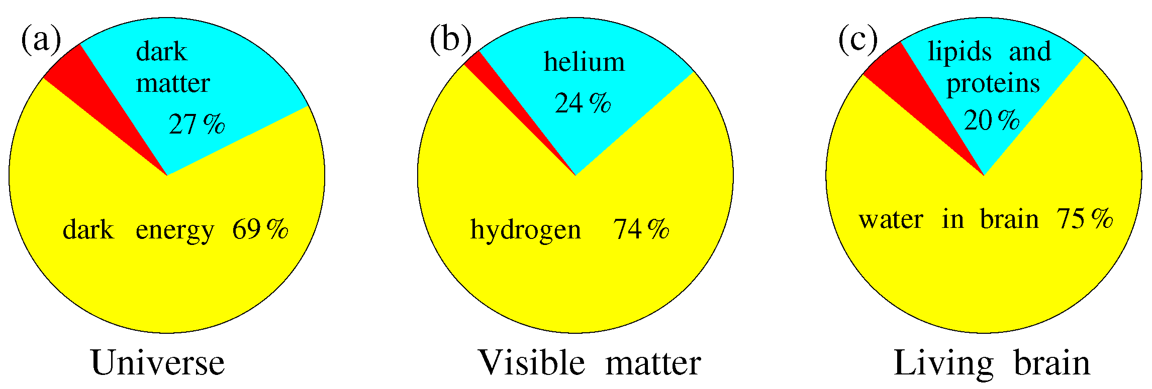
Figure 2.
A pair of proton-antiproton has opposite-oriented magnetic moments, and , and opposite directed momenta and . They revolve around the mass center staying on the mass shell.
Figure 2.
A pair of proton-antiproton has opposite-oriented magnetic moments, and , and opposite directed momenta and . They revolve around the mass center staying on the mass shell.
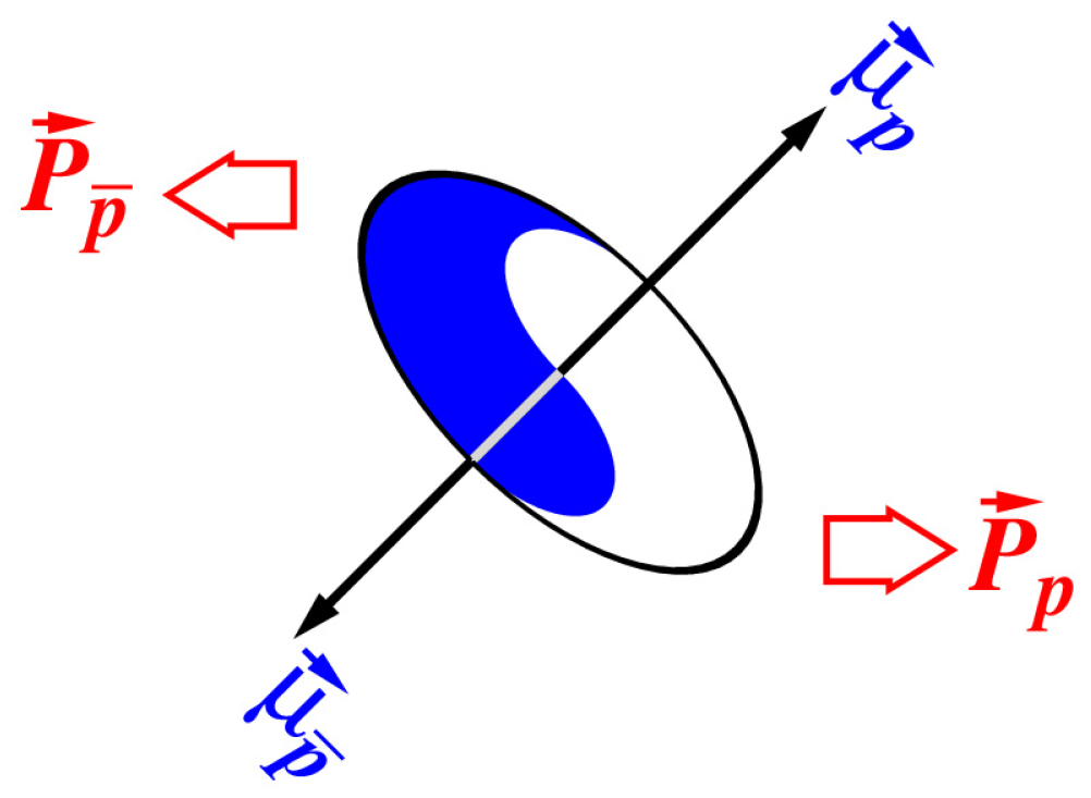
Figure 4.
Orbital velocity calculated by Eq. (42) at and : (a) , the Lamb-Oseen vortex decays quickly because of the large value of the viscosity coefficient; (b) , the decaying rate is slow because of the addition of this parameter. The larger this parameter, the slower the decay.
Figure 4.
Orbital velocity calculated by Eq. (42) at and : (a) , the Lamb-Oseen vortex decays quickly because of the large value of the viscosity coefficient; (b) , the decaying rate is slow because of the addition of this parameter. The larger this parameter, the slower the decay.
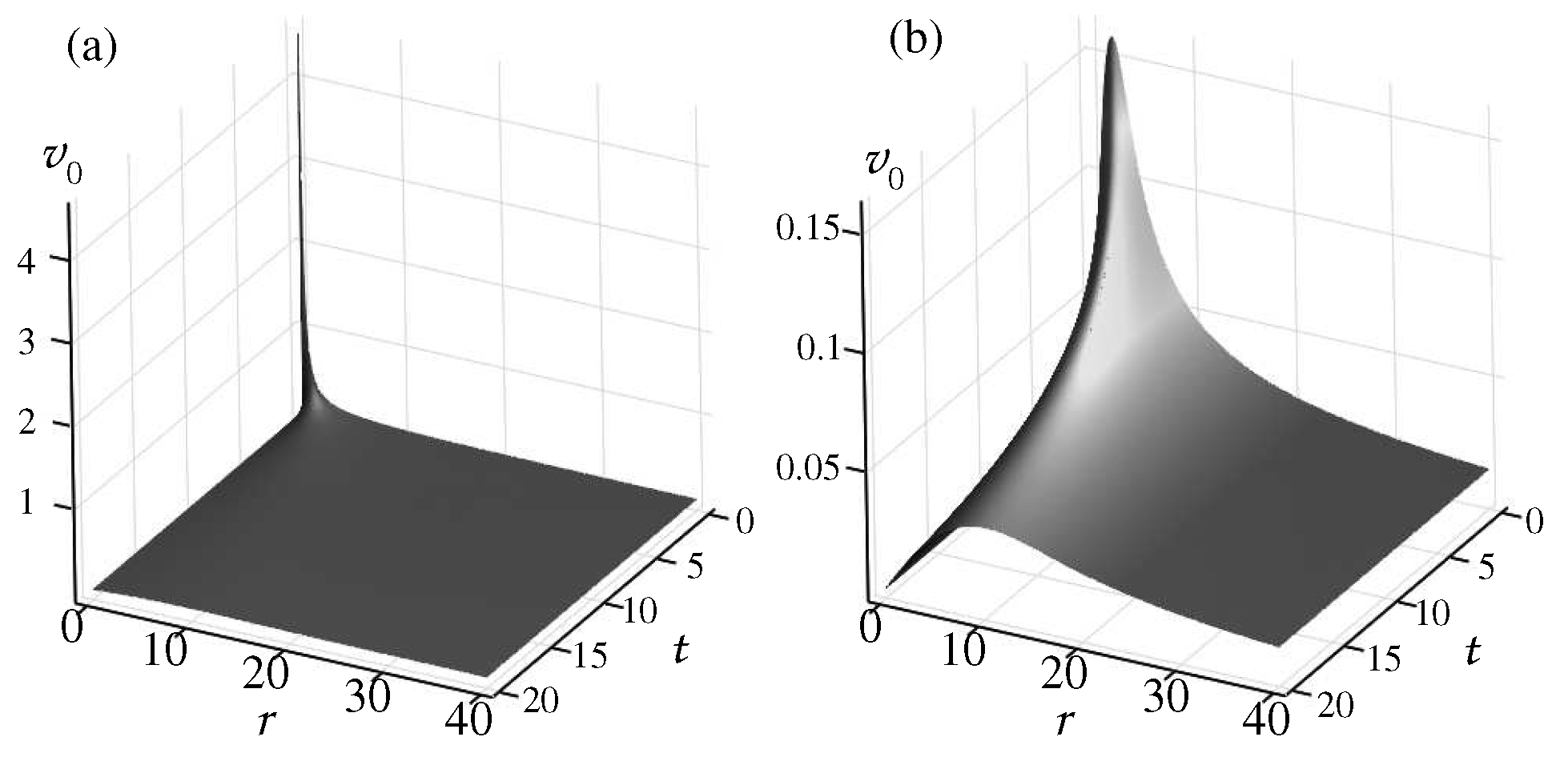
Figure 5.
Tangential velocity (44) loaded by the coefficients from (45) for (Lamb-Oseen vortex shown in Figure ??, curve (a)), , from the left to right, respectively.
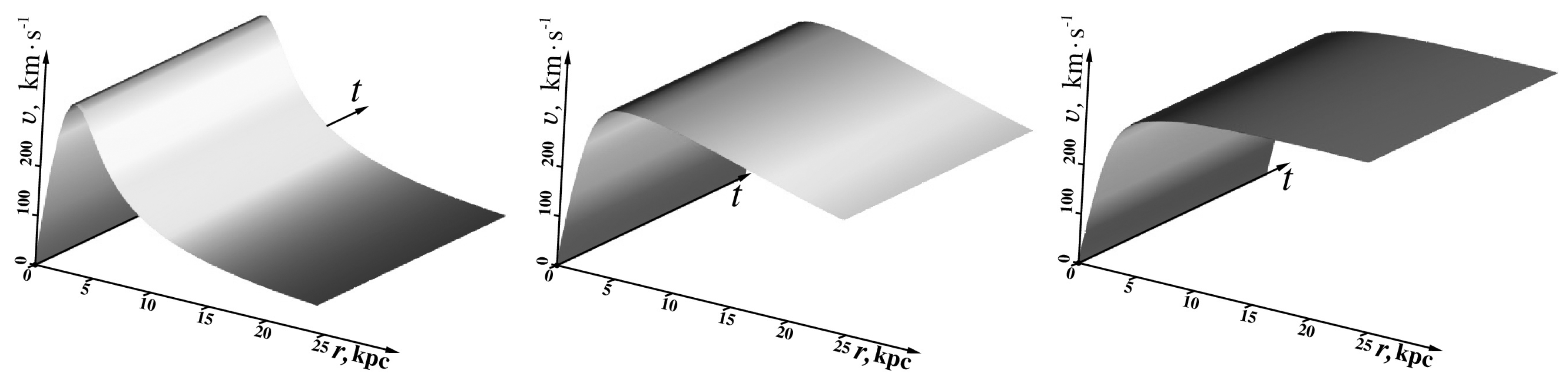
Figure 6.
Solenoidal speed as function of the radius r from the galactic center (in kiloparsec) and time t (in light years). The breathing of a galaxy is shown as the ripples of the flat plateau of the curve [77].
Figure 6.
Solenoidal speed as function of the radius r from the galactic center (in kiloparsec) and time t (in light years). The breathing of a galaxy is shown as the ripples of the flat plateau of the curve [77].
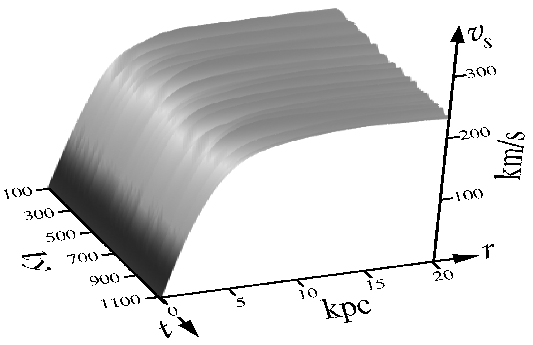
Figure 7.
Families F#, U#, and ESO# of the flat profiles of the orbital speeds taken from [72]. Red curves approximate profiles marked by black points.
Figure 7.
Families F#, U#, and ESO# of the flat profiles of the orbital speeds taken from [72]. Red curves approximate profiles marked by black points.
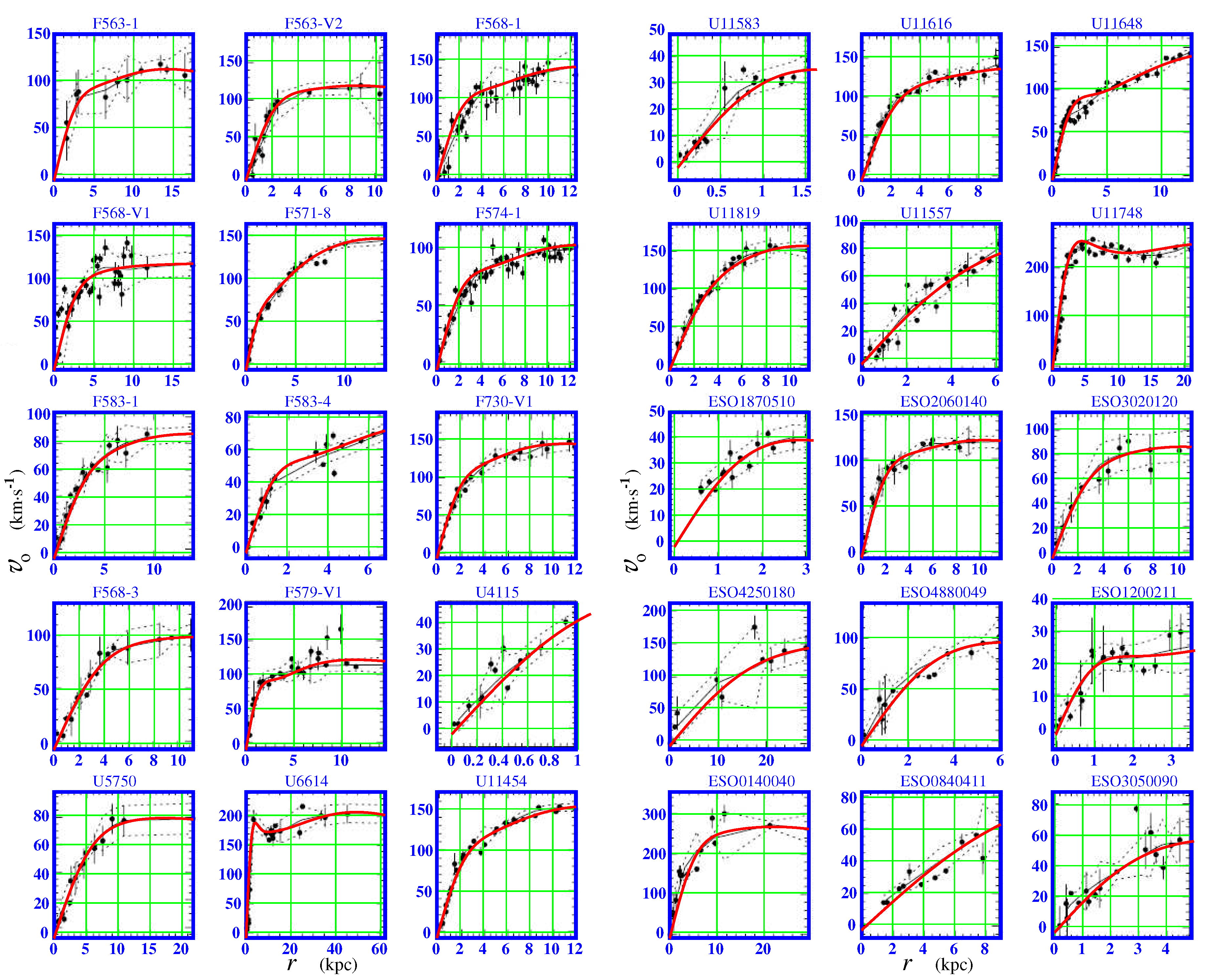
Figure 8.
Scheme of the Aharonov-Bohm experiment for the massive rotating disks placed in a deep vacuum between two beams radiated from source S [36].
Figure 8.
Scheme of the Aharonov-Bohm experiment for the massive rotating disks placed in a deep vacuum between two beams radiated from source S [36].
Disclaimer/Publisher’s Note: The statements, opinions and data contained in all publications are solely those of the individual author(s) and contributor(s) and not of MDPI and/or the editor(s). MDPI and/or the editor(s) disclaim responsibility for any injury to people or property resulting from any ideas, methods, instructions or products referred to in the content. |
© 2023 by the authors. Licensee MDPI, Basel, Switzerland. This article is an open access article distributed under the terms and conditions of the Creative Commons Attribution (CC BY) license (http://creativecommons.org/licenses/by/4.0/).
Copyright: This open access article is published under a Creative Commons CC BY 4.0 license, which permit the free download, distribution, and reuse, provided that the author and preprint are cited in any reuse.


