
Submitted:
26 November 2023
Posted:
27 November 2023
You are already at the latest version
Abstract
This study explores the application of numerical analysis and material models to predict ice impact loads on ships and offshore structures operating in polar regions. An explicit finite element analysis (FEA) approach was employed to simulate an ice and steel plate collision experiment conducted in a cold chamber. The pressure and strain history during the ice collision were calculated and compared with the experimental results. Various material model configurations were applied to the FEA to account for the versatile behavior of ice—whether ductile or brittle—its elastic-plastic yield criteria, and its dynamic strain rate dependency. In addition to the standard linear elastic perfectly plastic and linear elastic-plastic relationships, this study incorporated the crushable foam and Drucker-Prager models, based on the specific ice yield criteria. Considering the ice’s strain rate dependency, collision simulations were conducted for each yield criteria model to compute the strain and reaction force of the plate specimens. By comparing the predicted pressures for each material model combination with the pressures from ice collision experiments, our study proposes material models that consider the yielding, damage, and behavioral characteristics of ice. Lastly, our study proposes a combination of ice material properties that can accurately predict collision force.
Keywords:
ice collision force
; ice material behavior
; ice yield criteria
; ice strain-rate dependency
; crushable foam model
; Drucker-Prager model
1. Introduction
Vessels and offshore structures operating in Arctic regions constantly face the risk of structural damage from collisions with ice. A notable incident took place in January 1994, when the tanker Overseas Ohio, weighing 10,000 tons and traveling at approximately 5 m/s, sustained bow damage due to an ice collision off the coast of Alaska, resulting in severe marine pollution [1]. In the design phase of Arctic ships and offshore structures, predicting ice collision force is crucial for identifying structures with impact-resistant stiffness to minimize the risk of hull damage. This study introduces a numerical procedure and methodology for estimating ice collision force and compares the results with experimental findings to assess the validity of the load prediction process. The determination of collision forces can be categorized into two main analytical frameworks: dynamic structural analysis and fluid-structure interaction analysis. Several studies [2,3,4] have employed dynamic structural analysis to calculate ice collision force. Additionally, methods utilizing fluid-structure interaction to simulate ice-structure collisions have been explored [5], along with dynamic structural analyses focusing on the damage to both ice and structures [7,8]. Various constitutive equations and damage models for ice have been applied to predict collision force [3,9,10]. Despite the numerous approaches to ice collision force analysis discussed in the literature, this topic remains a subject of ongoing investigation. This continued interest is due to the significant variability in material properties, including elastic and plastic deformation and ice fracture, as well as the irregular changes in contact area during collisions, which pose significant challenges in accurately simulating ice damage and structural response. Different models have been applied to characterize the interactions between ice and other materials, including the Drucker-Prager model [11,12] and the crushable foam model [7,8]. However, variations in the ice-induced resistance faced by ships have been observed, highlighting the need to evaluate load predictions based on different yield criterion assumptions. Furthermore, studies using the discrete element method (DEM) have simultaneously considered the fragmentation of level ice during ship collisions, the formation and movement of ice blocks, and the interaction between ice blocks and ship structures [13,14,15]. Importantly, the DEM accounts for both ship and ice motion, including contact loading between individual ice blocks and the ship’s hull. Moreover, this approach represents the shape of ice as polygons or polyhedra and can simulate the mutual motion between ice and ship structure, as well as the ice fragmentation process. Models evaluating the impact of local ice collision force on ship structures, including various material properties and ice shapes, continue to attract considerable attention. Previous studies have conducted ice collision tests using various impact apparatuses. For example, Zhu et al. [7] and Cai et al. [8] conducted collision experiments with wedge-shaped ice specimens at speeds of 4 to 7 knots to measure the loads applied to the impacted bodies. Additionally, Jang et al. [16] presented the results of collision experiments between hemispherical ice specimens and steel plates using a collision pendulum at controlled speeds (5, 7, 10 knots) in a low-temperature chamber. These experiments accurately predict loads under experimental conditions, but they require scaling down the size of the ship and ice, and the experimental conditions are limited. In contrast, numerical simulation models do not account for size and shape limitations for ships and ice or collision speeds, but accuracy verification is essential. Therefore, numerical simulations must be performed to predict the ice collision force and to conduct analytical and experimental work for accuracy verification. The purpose of this study is to propose a procedure for numerically evaluating the local ice collision force and the response of steel plates by simulating simplified experiments. This procedure considers various factors, including yield criteria, material behavior, and strain rate effects in the material model of ice. To achieve this, several numerical simulations were conducted to reproduce the local collision force and structural deformation at the collision speeds realized in experiments. These simulations vary the material model to propose results and evaluate the impact of material properties on ice collision force predictions. This study also sought to expand the range of environmental variables associated with ice collision, (e.g., collision speed) in existing empirical design formulas to demonstrate the applicability of numerical analysis for load prediction. By systematically examining the performance of proposed material models against experimentally observed responses, this research aims to develop the appropriate numerical model for ice collision force prediction.
2. Material Properties of Ice
The strength and behavior of ice are strongly influenced by its crystal structure, salinity, temperature, and strain rate [17,18]. The determination of material properties and constants associated with ice deformation is uniquely challenging due to the complexity of the variables that influence this phenomenon. Numerous studies [3,5,9,19,20] have focused on the mechanical properties of ice, such as its constitutive relationships, fracture properties, and strain rate dependence, rather than the subtleties of its microstructure or thermal variations. Building on these findings, the present study incorporates the elastoplastic behavior, fracture characteristics, and strain rate sensitivity of ice. The referenced literature describes the mechanical properties of ice in detail, which are used as the basis for deriving the material properties and constitutive equations listed in Table 1. Therefore, this study sought to apply these data in an analytical framework where the results of different combinations of material properties can be compared and analyzed.
2.1. Constitutive Equations for Ice Elasto-Plastic Behavior
In the initial phase of this study, two different constitutive models were evaluated to characterize the elastic-plastic behavior of ice. The first constitutive model considered herein was the linear elastic-perfectly plastic with damage model (LEPP), dominated by elastic behavior. The second material model was the linear elastic-plastic with damage model (LEP), assuming plastic deformation as the primary response. The load-displacement curves for these models are depicted in Figure 1, illustrating a linear increase in behavior with applied load.
The LEPP model, which emphasizes the elastic domain, suggests that when the load is removed, the strain and stress are fully recoverable, indicating that no permanent deformation occurs until the yield strength ()) is reached. At the yield point, the material begins to suffer damage (Damage, D=0). This constitutes a crucial aspect of the model, as it marks the onset of fracture or failure in the ice structure. In contrast, the LEP model assumes a low yield stress threshold. Therefore, yielding occurs immediately upon loading, resulting in a negligible elastic phase. Consequently, after yielding, the ice does not return to its original state when the load is removed but continues to suffer damage until it reaches its ultimate strength (), at which point damage propagation becomes more pronounced. The adequacy of these two material models is discussed by comparing their predicted behavior with experimental observations. Finally, this study aims to compare the predictive capabilities of these two material models with experimental results to determine the most appropriate description of ice behavior.
2.2. Yield Criteria of Ice
- (1)
- Crushable foam model
The crushable foam model effectively represents the hardening characteristics associated with the volumetric strain of ice under compressive loading. This model has been successfully applied by researchers such as Gagnon & Derradji-Aouat [21], Kim et al. [4], Gagnon [3], and Gao et al. [22], and was also utilized by Obisesan & Sriramula [23] in their analyses. A key feature of the crushable foam model is the assumption that the material does not exhibit elastic recovery after yielding, resulting in permanent deformation. This model not only accounts for the failure stress associated with tension and compression but also considers the hardening characteristics. The yield surface () of the crushable foam model is defined by Equations (1) to (3) and is represented as an elliptical shape, as shown in Figure 2. Due to these characteristics, yielding occurs under the influence of hydrostatic compression pressures.
where and represent the major and minor axes of the elliptical yield surface in the crushable foam model, respectively, with denoting the center. and denote the yield strengths under hydrostatic compression and hydrostatic tension conditions, respectively. The factor represents the ratio of yield in compression, whereas represents the ratio of yield under hydrostatic conditions. The initial yield stress in hydrostatic conditions is indicated by , whereas represents the uniaxial compressive yield stress, which is shown in Figure 2 as the point where the yield surface intersects the -axis. As the deformation of the ice enters the plastic regime, the size and shape of the yield surface change; this change can be expressed by the relationship between the uniaxial compressive yield stress and the volumetric strain. These changes are described by a strain hardening model where the yield surface varies based on a line connecting and intersecting with the axis. The evolution of the yield surface can be represented as a function of the volumetric plastic hardening, , as expressed in Equation (4), which expresses the relationship between the volumetric plasticity and uniaxial stress. Volumetric hardening assumes that uniaxial plastic deformation () is equivalent to volumetric deformation (). To implement the hardening of the crushable foam plastic model in ABAQUS, the change in the yield surface is reflected by the uniaxial compressive yield stress and plastic strain rate.
- (2)
- Drucker-Prager model
The Drucker-Prager model is known to be suitable for materials with internal friction, such as rock and concrete. This model effectively captures the strengthening of certain materials under compressive loads and is appropriate for describing the behavior of materials where the compressive strength is higher than the tensile strength. Noting the similarity between the behavior of ice and concrete, Kajaste-Rudnitski & Kujala [11], as well as Zhang et al. [12], have applied the Drucker-Prager approach to ice collision models. A key feature of the Drucker-Prager model is its use of a non-circular yield surface to adjust the yield stress values in both tensile and compressive scenarios. This model allows for the independent setting of the dilation and friction angles, and as shown in Figure 3, it defines the yield surface through three invariants. The yield surface () of the Drucker-Prager model can be expressed as described in Equations (5), (6), and (7).
where represents the material’s angle of friction in the - plane, denotes the material’s cohesion, is the ratio of the triaxial tensile yield stress to the triaxial compressive yield stress, is the equivalent pressure, and represents the Von-Mises stress. In other words, the yield condition of the Drucker-Prager model typically takes on a non-circular form, with the yield surface determined by the material’s angle of friction (), cohesion (), equivalent pressure (), and Von-Mises stress (). The study by Kajaste-Rudnitski & Kujala [11] provides a detailed application of such a model.
- (3)
- Ductile damage model
Material failure or damage is defined as the gradual deterioration of a material’s stiffness, resulting in a complete loss of load-carrying capacity. To address this behavior in ice, a ductile damage model was adopted in this study. Fracture-based theory illustrates the stress-strain behavior of the material, as depicted in Figure 4.
- Damage Initiation (D=0): The fracture model identifies the commencement of damage when the material reaches its ultimate strength. Damage initiation is typically associated with the equivalent plastic strain ().
- Damage Evolution (0<D<1): In Figure 4, the dotted line represents the undamaged response, indicating the material’s pure plastic behavior without the influence of a damage model. The solid line, labeled as “softening,” depicts the behavior of the material once it has sustained damage. Following damage initiation (D=0), the model simulates the progression of damage. As the damage evolves, the material’s stiffness starts to decrease, and the damage variable (D) increases.
- Fracture (D=1): When the damage variable (D) reaches 1, signifying the completion of the damage progression, the material’s internal cohesive strength is completely lost. At this point, material fracture occurs, and bonded elements may separate or be removed (i.e., element deletion).
2.3. Strain Rate Dependency of Ice: Yield Strength Ratio
This section examines the complex relationship between yield strength ratio and strain rate. Notably, higher strain rates typically lead to an increase in the yield strength of ice, as highlighted by Tippmann [24]. Moreover, Barette and Jordaan [17] reported that lower temperatures also contribute to an increase in the intrinsic strength of ice. It is also important to consider that both strain rate and yield stress tend to increase simultaneously as collision energy increases. Tippmann [24] explored these dynamics by investigating interactions between ice and structural elements, particularly in scenarios involving spherical ice specimens colliding with carbon fiber-reinforced plastic (CFRP) plates. Furthermore, in the context of high-velocity collisions, it is important to account for the strain rate dependence of the materials involved. This aspect has been addressed by adopting the model proposed by Tippmann [24]. Notably, the range of strain rates outlined by Tippmann [24] extends beyond the strain rate of this study, enabling the analysis of a broader spectrum of collision velocities. Based on observations from collision experiments with ice, it is evident that yield strength is dependent on strain rate. Tippmann [24] and Tippmann et al. [25] conducted studies focusing on this dependency, analyzing the relationship between strain rate and yield strength. Their findings demonstrated that as the strain rate increases, the compressive strength also shows an upward trend. During the plastic deformation of ice, yield occurs at a specific strain rate, after which the stress remains relatively constant. This phenomenon is particularly observed during high-speed ice collisions, making a perfect plasticity model appropriate, assuming a yield hardening coefficient of 0 [26,27]. Tippmann [24] and Tippmann et al. [25] compiled various research data and represented the relationship between strain rate and yield strength using a linear-logarithmic curve. In this study, this relationship, specifically the ‘strain rate-yield ratio,’ was incorporated into the analysis. Figure 5 illustrates the relationship between compressive plastic strength and the yield strength ration within a strain rate range of 0.1/s to 106/s, providing a visual representation of this curve and the relevant values. The yield strength ratio is normalized to the initial compressive plastic strength of 5.2 MPa.
3. Ice material Calibration
In the previous section, various material properties of ice were described, focusing on plastic deformation relationships, yield conditions, and the strain rate dependency of yield strength. As reported in previous studies, different models are employed for different material properties, reflecting the complex and uncertain nature of the deformation properties of ice. In this section, considering the diversity of material models mentioned in Section 2, the selection process for material models and material constants that can account for the dynamic compressive deformation characteristics of ice is presented.
- Plastic deformation relationships: Models such as the linear elastic-perfectly plastic (LEPP) and linear elastic-plastic (LEP) models define how materials behave when they exceed the elastic limit. While the LEPP model assumes that no deformation occurs beyond the yield point, the LEP model describes post-yield hardening or softening. These material plastic properties are applied to the analyses to verify their results.
- Yield criteria: The crushable foam (CF) and Drucker-Prager (DP) models define the conditions under which materials reach yield. The CF model simulates the collapse of cellular materials under compression, whereas the DP model models the yield of pressure-dependent materials. Given the sensitivity of ice to pressure and density, the appropriateness of these conditions was investigated.
- Strain rate dependence: In dynamic events such as collisions, strain rate affects the yield stress and failure modes of the material. Results are analyzed based on whether or not strain rate dependence is considered.
In this study, the combination of these three models was applied to material modeling efforts and compared with experimental data to select the most appropriate model. This approach helps to reduce the complexity and uncertainty associated with material modeling and allows for more accurate predictions of ice behavior in real-world scenarios. In this study, four models were adopted by combining (1) two plastic constitutive equations and (2) two yield conditions. Additionally, (3) the effects of strain rate are included in all eight material model combinations, as summarized in Table 2. Determining material constants for the ICE material models, including elasticity coefficients, yield stresses, hardening coefficients, and yield strength ratios, typically requires performing tensile tests, bending tests, or triaxial compression tests. In some cases, these constants can be indirectly estimated through theoretical analysis. In this research, however, these values were derived by performing quasi-static compression experiments on ice and simulating these experiments using finite element analysis. A detailed description of this process is provided in Section 3.1 and Section 3.2. Additionally, the compression strength ratio as a function of strain rate, as measured by Tippmann [24] in high-speed collisions with CFRP, was used to assess the dynamic deformation properties of ice with strain rate dependence. The values required to define the strain rate dependence are provided in Figure 5 of the previous section, with the lower limit of the compression strength ratio curve being applied.
3.1. Determination of Material Model Constants
This section discusses the process of determining the material constants required for the elastic constitutive equations (i.e., linear elastic deformation relations) for ice, including the LEPP and LEP models, as well as the yield conditions required for the CF and DP models. The constants that must be defined for each material model are summarized below:
- LEPP model: This model requires the determination of two fundamental material constants, Young’s modulus () and the yield stress (). Young’s modulus is conventionally obtained from tensile tests, whereas the yield stress is the stress point at which the material begins to undergo plastic deformation.
- LEP model: Similar to LEPP, the LEP model requires the determination of Young’s modulus () and yield stress (). In addition, it requires consideration of additional constants associated with the hardening model and the hardening coefficient or plastic flow rule.
- CF model: This model requires the definition of material constants that govern the compressive behavior of foams. Key constants include density, initial strength (), and hardening coefficient. The determination of these constants is facilitated by the analysis of stress-strain curves derived from compression tests on specimens.
- DP model: The DP model requires a set of constants related to the angle of internal friction (β), material cohesion (d), drag parameters such as the dilatancy angle (ψ), and constants related to the hardening rule. Typically, these constants are obtained from triaxial compression tests and should be considered in conjunction with stress paths.
For material constants that are difficult to measure or calculate directly, assumptions were made based on existing literature. Specifically, values from Tippmann [24], Kajaste-Rudnitski & Kujala [11], Zhang et al. [12], Kim et al. [4], and Han et al. [9] were used to set the density and Poisson’s ratio of ice to 900 kg/m³ and 0.3, respectively. Undetermined material constants for the CF and DP models were hypothetically varied and then incorporated into finite element analyses, ultimately yielding material constants consistent with experimental results. It should be noted, however, that the material models applied to quasi-static compression simulations, which primarily represent low rates of deformation, are tailored to exhibit characteristics specific to quasi-static compression. The constants that define the yield criteria, including parameters associated with damage initiation and stiffness reduction after initiation, are taken from the works of Obisesan & Sriramula [23] and Jeon & Kim [20]. The determined parameters for the yielding models are summarized in Table 3. Additionally, the undetermined material constants specific to each material model were refined to best match the experimental results through simulation analyses simulating ice compression tests, as described in Section 3.2. The material constants defined in the ice compression simulations are as follows:
- LEPP model: The apparent elastic modulus was assumed to be 0.14 GPa. The yield stresses for the CF and DP models were set at 4.8 MPa and 3 MPa respectively. The material damage model parameters included a failure strain of 1.0 × 10⁻⁴ and an energy release rate of 15.0 J.
- LEP model: The elastic modulus, influenced by stress and strain rate, was set to 9 GPa. Hardening constants for this model are detailed in Table 4 for both the CF and DP models, and failure strains were designated as 0.019 and 0.025, respectively, with a damage evolution energy of 15.0 J.
These material constants were carefully tuned to accurately simulate the ice compression behavior under the chosen material models.
3.2. Finite Element Analysis Simulating Ice Compression Experiments
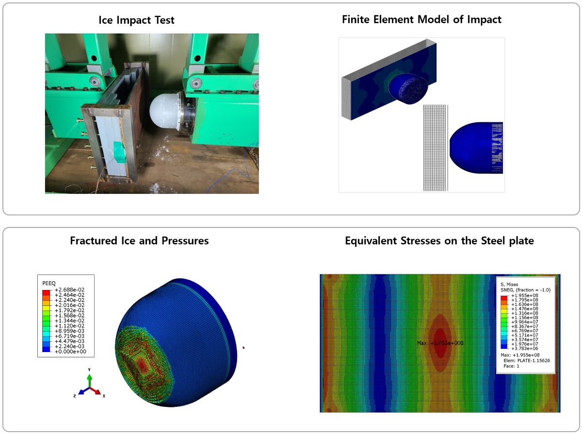
This study successfully conducted quasi-static compression tests on ice specimens using compression testing equipment, which enabled the validation of specific material constants. Building on these experiments, finite element analysis (FEA) was then performed. Throughout this process, multiple FEA iterations were undertaken to determine previously undefined material constants. According to the quasi-static compression test results reported by Jang et al. [16], it was observed that ice specimens, configured as square columns with cross-sectional dimensions of 100 mm × 100 mm and a height of 250 mm, failed under loads ranging from approximately 25 to 32 kN when compressed by 5 mm (Figure 6).
For the finite element modeling, these specimens were represented using 39,375 solid elements (C3D8R), with each element having a grid size of 4 mm. The compression plate in the model was assumed to be a rigid body (Figure 7). The setup for the analysis model was as follows:
- Contact conditions: The lower surface of the ice specimen was fixed in place. A hard node-to-surface contact condition was applied to the upper surface, which came into contact with the rigid compression plate. This setup was crucial to prevent any penetration between the specimen and the plate.
- Compression conditions: The rigid compression plate was set to move at a speed of 1.0 mm/s, mirroring the experimental conditions. This movement applied a controlled displacement to the specimen, thereby replicating the actual test conditions in the numerical model.
The quasi-static compression experiments on ice were reproduced using finite element analysis models to calculate the load and displacement values leading to failure. Verification was achieved through a comparison with experimental results. One of the primary objectives of this study was to optimize the material constants for each finite element model to accurately reproduce the average failure load of 28 kN, as observed in the experiments. This involved finely tuning various material constants, including yield stress, hardening coefficient, and parameters of the damage model. The aim was to ensure that the predicted load-displacement relationship derived from the FEA closely matched the experimental data, maintaining an error margin of less than 1.5%.
In the experimental setup, the reaction force corresponding to the displacement was measured. In contrast, the total compression load acting on the bottom surface of the ice was calculated via FEA. Through iterative processes, the material constants were precisely adjusted to align with experimental observations. The refined load-displacement relationships for each material model are depicted in Figure 8. Table 5 summarizes the compression loads at specific points, confirming that the material constants deduced in this study effectively replicate the ice compression behavior observed in the experiments.
4. Simulation Model for the Ice-Structure Collision Experiment
In this study, the analysis of ice-structure collisions is divided into two aspects: ice damage and the dynamic response of the structure. Explicit finite element analysis was conducted to investigate these aspects. The commercial software ABAQUS/Explicit was used to simulate the nonlinear dynamic response during the collision process between the two objects. Solid elements (C3D8R) were chosen to represent the yielding and failure behavior of the ice, whereas the structure was represented by shell elements (S4R). The main features of this finite element analysis model are explained below:
- Ice yield criteria: The CF and DP models were used to model the yielding and failure behavior of ice, as described in Section 2.1.
- Contact conditions: Contact conditions were established to account for the interaction between the two objects and to calculate the load transferred from the ice to the structure. For the contact between ice elements and plates, hard contact and tie conditions are applied.
- Element with reduced integration: Reduced integration was used to establish the stiffness matrix to enhance the computational efficiency, along with the selection of the hourglass control.
- Time increment: In the explicit finite element analysis, the determination of the time increment (△t) is crucial for achieving both accuracy and computational efficiency. In our study, the time increment for explicit integration was calculated using the following formula: , where represents the size of the smallest element within mesh. Moreover, represents the material’s dilatational wave speed, which is a function of the material’s mechanical properties and is calculated using the formula: , where E denotes the elastic modulus of the material, and ρ denotes the density.
Both quasi-static material models and dynamic material models, which account for strain rate effects were discussed in the previous section, were applied in the analysis. Analyses were conducted for each yield model considered, and the obtained strain and ice load on the plate were compared with the experimental values. This study encompasses four distinct material models: the LEPP, LEP, CF, and DP models. These models are integrated into the FEA to assess and compare the fidelity of ice collision simulations across each material model. This comparative analysis aims to identify the most accurate model in simulating the behavior of ice-structure impact.
4.1. Overview of the Ice-Structural Collision Simulation Model
In this study, the collision pendulum experiment conducted by Jang et al. [16] was chosen for numerical simulation. A detailed discussion on the material models associated this simulation is provided in Section 2, Section 3.1, and Section 3.2. Figure 9 (left) shows the ice specimen, the impactor, and the specimen holder used in the experiment. Correspondingly, the finite element model (FEM) mirrors the geometry of the ice and steel plate specimens, as well as the specimen holder. Figure 9 (right) illustrates the analysis model, which incorporates the experimental apparatus. The dynamic behavior of collision and the steel plate’s response are simulated using an explicit scheme of FEM. The mesh of the FEM is presented on the Figure 9 (b). The collision velocities tested in the experiment, specifically 2.5, 3.5, and 5 knots, were applied to the FEA, which spans a duration of 0.05 seconds.
Figure 10 and Figure 11 illustrate the configurations of the ice specimen and holder, as well as the steel plate and its corresponding jig, respectively. The ice specimen is modeled as a hemisphere with a 250 mm height and a 300 mm diameter, represented by solid elements in the simulation. The total weight of the ice holder, including the pendulum’s mass, was defined as 150 kg. The steel plate, with dimensions of 1,000 × 500 mm and a thickness of 20 mm, was modeled using shell elements. Additionally, the jig for supporting the steel plate was assumed as a rigid body, measuring 200 × 500 × 50 mm. At the interfaces where the ice specimen contacts the holder and the steel plate contacts the jig, node-to-surface contact with hard contact and frictionless conditions were implemented. In these contact conditions, the steel plate specimen, which possesses higher rigidity, was designated as the master surface. Additionally, tie contact conditions were established between the ice specimen and its holder, and between the steel plate specimen and its jig. Table 6 summarizes the shapes and conditions of each component employed in the analysis. A critical aspect of our analysis involved assessing mesh convergence. During the analysis process, mesh convergence was examined, and the effect of mesh size on the collision force was investigated by varying the ice grid size from 2 to 7 mm. The results indicated that a biased mesh size of 2–5 mm was the most appropriate.
4.2. Collision Analysis Reflecting Quasi-Static Compressed Material Model
The four material models introduced in Section 3.1 were applied to the analyses for specific collision velocities. However, this section did not include the dynamic strain rate effect of ice. Four separate analyses corresponding to a collision velocity of 10 knots were conducted, with the predicted shapes and stresses of the specimen deformation presented in Figure 12, Figure 13, and Figure 14. The top portions of each figure display the results using the LEPP model coupled with the CF and DP yield models. The bottom portions of each figure represent the results calculated with the LEP model of the ice material coupled with the CF and DP yield models, respectively. Interesting results were obtained when the CF yield model was applied to the LEPP model. In this case, the analysis results reveal the generation of large fragments due to spalling following the collision. On the other hand, the remaining three analysis models produce smaller fragments, which were more consistent with crushing phenomena. Significant differences in the observed loads during collision were noted depending on the characteristics of the analyzed fragments. Particularly, the model where large fragments were generated due to spalling exhibited significant deviations from the actual experimental results. These results underscore the importance of material model selection and its influence on collision analysis.
- Predicted strains on steel plate
Figure 15 and Figure 16 illustrate the strain rate history in the width direction and height direction of the plate specimen for various collision velocities. The maximum strain rates for ice properties based on collision velocity are summarized in Table 7, Table 8, and Figure 17. Both the LEPP and LEP models, in combination with the DP yield model, performed better than the combination with the CF model. Among these, the LEP model exhibited results closest to the experimental data, with error rates within 15%.
- Ice collision force prediction results
Figure 18 presents the collision force history applied to the plate specimen for various collision velocities. Figure 19 and Table 9 summarize the maximum collision force in conjunction with the strain rate for different material model combinations. Similar to the strain rate prediction results, the DP yield model outperformed the CF model in terms of accuracy. Particularly, the combination involving the LEP model exhibited a deviation of 22.1% from the experimental results. Among the material properties obtained from quasi-static compression experiments (W/O strain rate effect), this combination proved to be the closest to the experimental results. These results emphasize the significance of material model selection in collision-related analyses and highlight the importance of choosing a model that accurately predicts responses under various conditions.
4.3. Collision Analysis Reflecting Yield Ratio According to Strain Rate
This section presents the results of collision analysis, including the dynamic material properties of ice as a function of strain rate, as well as the models introduced in Section 4.1. Initially, the four material models introduced earlier were applied to calculate collision force and strain rates. The analysis was conducted for a collision velocity of 10 knots, and the calculated deformation shapes of the specimens are presented in Figure 21, Figure 21 and Figure 22. Figure 20 illustrates the failure pattern of ice predicted by combining the LEPP ice material model with the CF and DP yield models. Figure 21 illustrates the plastic strain distribution on the ice surface after the collision, whereas Figure 22 displays the Mises equivalent stress in the plate specimen. The analysis that combines LEP with the CF yield model does not consider the yield ratio in relation to strain rate. However, the analysis in Section 4.1 confirmed that the strain rate on the collision surface falls within a 20–30 mm/mm range. Based on the relationship between strain rate and yield strength ratio presented in Figure 5, the yield stress ratio could be estimated as 2.5. Additionally, the analysis that combined the LEPP model with the DP yield model illustrated the formation of spalling phenomena and the generation of large, fragmented particles.
- Strain of steel plate prediction results
The strain rate histories in the width and height directions of the plate specimen for various collision velocities are presented in Figure 23 and Figure 24, respectively. Figure 25 illustrates the maximum strain rates as a function of collision velocity for each material model. Detailed strain rate values are summarized in Table 10 and Table 11. Consistent with the results of the previous section, the DP yield model exhibited higher accuracy than the CF model. Among these models, the material model associated with the LPE model, which emphasizes plastic behavior, exhibited a lower deviation from the experimental results, with differences of 8.7% and 12.4%.
- Ice collision force prediction results
Figure 26 illustrates the history of collision force applied to the plate specimen as a function of collision velocity. The maximum strain rates for each material model are summarized in Figure 27 and Table 12. The DP yield model accurately predicted the ice loads applied to the plate specimen, outperforming the CF model. Furthermore, the material model associated with the LEP model, which accentuates plastic behavior, showed a deviation of 12.2% from the experimental results. This indicates a better fit compared to models that do not account for strain rate effects.
4.4. Evaluation of Suitability for each Combination of Ice Material Models
In this section, we compare the analysis results from Sections 3.3 and 3.4 with experimental data, summarizing the suitability of the analysis for each combination of material models. Below, the accuracies of the strain rate and collision force predictions for each ice material model are summarized.
- The strain rates for each material model were compared to identify models that closely match the experimental results. Figure 28 presents a comparison of the accuracy of the maximum strain rates in the width and height directions of the plate specimen as a function of collision velocity. Table 13 and Table 14 provide a comparison of the calculated and experimental values for the horizontal strain and vertical strain for each analysis combination. Here, we observed that dynamic material properties combined with the DP model (LEP-DP) accurately simulated , with an 8.7% deviation, and , with a 12.4% deviation. In summary, our findings demonstrated that considering dynamic effects yields better strain rate predictions, and when considering both width and height directions, the combination of the dynamic material properties of ice with the DP model is deemed the most appropriate model.

Table 13.
Comparison between the experimental and FEA-derived maximum strain x ().
| Collision velocity |
LEP-CF | LEP-DP | LEP-CF + Strain rate effect |
LEP-DP + Strain rate effect |
|---|---|---|---|---|
| 5 kts | 6.90 × 10⁻⁴ (7.1%) | 6.43 × 10⁻⁴ (0.2%) | 5.59 × 10⁻⁴ (13.2%) | 7.55 × 10⁻⁴ (−17.3%) |
| 7 kts | 8.06 × 10⁻⁴ (8.9%) | 8.63 × 10⁻⁴ (2.3%) | 7.22 × 10⁻⁴ (18.4%) | 8.26 × 10⁻⁴ (6.7%) |
| 10 kts | 1.17 × 10⁻³ (8.3%) | 1.11 × 10⁻³ (2.8%) | 8.26 × 10⁻⁴ (6.7%) | 1.06 × 10⁻³ (2.0%) |
| Avg. Difference |
8.1% | 1.7% | 15.0% | 8.7% |
Table 14.
Comparison of maximum strain y () from experiment and FEA.
| Collision Velocity |
LEP-CF | LEP-DP | LEP-CF + Strain rate effect |
LEP-DP + Strain rate effect |
|---|---|---|---|---|
| 5 kts | 2.80 × 10⁻⁴ (31.7%) | 2.40 × 10⁻⁴ (41.5%) | 2.96 × 10⁻⁴ (27.9%) | 3.32 × 10⁻⁴ (19.0%) |
| 7 kts | 3.12 × 10⁻⁴ (21.2%) | 2.99 × 10⁻⁴ (24.5%) | 2.90 × 10⁻⁴ (26.8%) | 3.92 × 10⁻⁴ (0.90%) |
| 10 kts | 5.53 × 10⁻³ (47.9%) | 3.76 × 10⁻³ (0.5%) | 3.80 × 10⁻⁴ (−1.5%) | 4.39 × 10⁻³ (−17.4%) |
| Avg. Difference |
33.6% | 22.1% | 17.7% | 12.4% |
- Subsequently, we turned our attention to the maximum collision force exerted by the ice on the plate specimen. The maximum collision force applied by the ice to the plate specimen was compared for different ice material property models. Figure 29 compares the predicted collision force for each material model combination against the experimental data.
- Table 15 provides a comprehensive summary of the differences between experimental and analytical collision force for each material model combination. The inclusion of dynamic strain rate effects to the LEP material model with the DP yield condition (LEP-DP with strain rate effect) accurately predicts collision force with a 12.2% deviation, demonstrating high accuracy in both strain rates and collision force. This material model combination shows high accuracy in both strain rates and collision force.
Overall, upon comparing the different numerical analysis configurations analyzed in this study, our findings demonstrated that the LEP material model, combining the DP yield condition and strain rate effects, best matches the experimental results. Table 16 summarizes the comparison between both strain rates and collision force values obtained through experiments and numerical modeling. Notably, the strain rate effects in the analysis results were very similar to the experimental results, with deviations of 8.7% for , 12.4% for , and 12.2% for collision force. Therefore, our findings confirmed that the ice material properties formulated by combining the DP yield condition and strain rate-yield strength ratio within the LEP material model best approximate the results of the ice collision experiments.
Table 15.
Comparison between the experimental and FEA-derived maximum force.
| Collision Velocity |
LEP-CF | LEP-DP | LEP-CF + Strain rate effect |
LEP-DP + Strain rate effect |
|---|---|---|---|---|
| 5 kts | 31.5 (2.9%) | 31.1 (4.2%) | 27.5 (25.0%) | 36.5 (-12.6%) |
| 7 kts | 44.7 (1.3%) | 42.7 (5.7%) | 36.9 (18.5%) | 39.9 (11.8%) |
| 10 kts | 68.8 (3.7%) | 63.9 (10.5%) | 52.8 (25.0%) | 61.8 (12.2%) |
| Avg. Difference |
2.6% | 6.8% | 19.5% | 12.2% |
Table 16.
Comparative summary of the experimental and FEA-derived results.
| FEA Result | Material model | 5 kts | 7 kts | 10 kts | Mean Diff. |
|---|---|---|---|---|---|
|
) (Difference with experiment) |
LEP -DP |
(−13.2%) |
(−18.4%) |
(−6.7%) |
15.0% |
| LEP -DP + Strain rate effect |
(−17.3%) |
(−6.7%) |
(−2.0%) |
8.7% | |
|
) (Difference with experiment) |
LEP -DP |
(−27.9%) |
(−26.8%) |
(−1.5%) |
17.7% |
| LEP -DP + Strain rate effect |
(−19.0%) |
(−0.9%) |
(−17.4%) |
12.4% | |
| Max. force (Difference with experiment) |
LEP -DP | 27.5 (−25.0%) |
36.9 (−18.5%) |
52.8 (−25.0%) |
19.5% |
| LEP -DP + Strain rate effect |
36.5 (−12.6%) |
39.9 (−11.8%) |
61.8 (−12.2%) |
12.2% |
5. Conclusion
This study reviews various material models and numerical simulation methodologies relevant to the impact of ice on structures, with a focus on developing a sophisticated numerical simulation model capable of accurately capturing the pressure characteristics induced by ice impacts. Using dynamic explicit finite element analysis, this study incorporated the elastic-plastic material properties of ice specimens, the effect of strain rate, yield condition, and the fracture behavior of materials. Initial analyses were conducted to validate necessary material constants for each ice material model, serving as a foundation for subsequent finite element simulations of ice impact scenarios. These simulations were iteratively refined to align closely with empirical impact load. The analysis process entailed exploring combinations of various material models. These included the linear elastic-perfectly plastic relationship, the linear elastic-plastic relationship, the crushable foam model, and the Drucker-Prager model, along with considering the strain rate dependency of ice. Collision simulations were instrumental in computing the strain and reaction forces of plate specimens, which were then compared with values measured in collision experiments. Our findings suggest that a material model that incorporates the Drucker-Prager yield criterion and a dynamic yield ratio within a Linear Elastic-Plastic framework most accurately reflects the experimental results. This study sought to validate the feasibility of simulating experiments with different material models of ice, which are essential for the analysis of ice-structure interactions. The validation of this numerical model enhances the predictive capabilities for offshore structural loads and allows for the derivation of more realistic ice material models through empirical comparisons.
Author Contributions
J.H.L. managed the project and provided supervision; S.H. designed the methodology and suggested a FEA procedure; H.-S.J. performed the research and validation of ice collision FEA; H.-S.J. and J.Y. performed formal analysis and visualization of FEA results; H.-S.J. and J.H.L. wrote the paper. All authors have read and agreed to the published version of the manuscript.
Funding
This research was supported by the Korea Institute for Advancement of Technology (KIAT) grant funded by the Korean Government (MOTIE) (P0023684, HRD Program for Industrial Innovation)
Institutional Review Board Statement
Not applicable.
Informed Consent Statement
Not applicable.
Data Availability Statement
Not applicable.
Acknowledgments
This research was supported by the Korea Institute for Advancement of Technology (KIAT) grant funded by the Korea Government (MOTIE) (P0023684, HRD Program for Industrial Innovation).
Conflicts of Interest
The authors declare no conflicts of interest.
References
- Tangborn, A.; Kan, S.; Tangborn, W. Calculation of the Size of the Iceberg Struck by the Oil tanker Overseas Ohio. In 14th IAHR Symposium on Ice, 1998; Vol. 1, pp 237-241.
- Gagnon, R. Results of numerical simulations of growler impact tests. Cold Reg. Sci. Technol. 2007, 49(3), 206–214. [Google Scholar] [CrossRef]
- Gagnon, R. A numerical model of ice crushing using a foam analogue. Cold Reg. Sci. Technol. 2011, 65(3), 335–350. [Google Scholar] [CrossRef]
- Kim, H.; Daley, C.; Colbourne, B. A numerical model for ice crushing on concave surfaces. Ocean Eng. 2015, 106, 289–297. [Google Scholar] [CrossRef]
- Kajaste-Rudnitski, J.; Kujala, P. Ship propagation through ice field. J. Struct. Mech. 2014, 47(2), 34–49. [Google Scholar]
- Song, M.; Kim, E.; Amdahl, J. Fluid-structure-interaction analysis of an ice block-structure collision. 2015.
- Zhu, L.; Qiu, X.; Chen, M.; Yu, T. Simplified ship-ice collision numerical simulations. In ISOPE International Ocean and Polar Engineering Conference, 2016; ISOPE: pp ISOPE-I-16-521.
- Cai, W.; Zhu, L.; Yu, T.; Li, Y. Numerical simulations for plates under ice impact based on a concrete constitutive ice model. Int. J. Impact Eng. 2020, 143, 103594. [Google Scholar] [CrossRef]
- Han, D.; Lee, H.; Choung, J.; Kim, H.; Daley, C. Cone ice crushing tests and simulations associated with various yield and fracture criteria. Ships and Offshore Structures 2017, 12 (sup1), S88–S99. [Google Scholar] [CrossRef]
- Gutfraind, R.; Savage, S. B. Smoothed particle hydrodynamics for the simulation of broken-ice fields: Mohr–Coulomb-type rheology and frictional boundary conditions. J. Comput. Phys. 1997, 134(2), 203–215. [Google Scholar] [CrossRef]
- Kajaste-Rudnitski, J.; Kujala, P. Ship propagation through ice field. J. Struct. Mech. 2014, 47(2), 34–49. [Google Scholar]
- Zhang, N.; Zheng, X.; Ma, Q. Updated smoothed particle hydrodynamics for simulating bending and compression failure progress of ice. Water 2017, 9(11), 882. [Google Scholar] [CrossRef]
- Tuhkuri, J.; Polojärvi, A. A review of discrete element simulation of ice–structure interaction. Philosophical Transactions of the Royal Society A: Mathematical. Phys. Eng. Sci. 2018, 376(2129), 20170335. [Google Scholar]
- Tsarau, A.; Lubbad, R.; Løset, S. A numerical model for simulation of the hydrodynamic interactions between a marine floater and fragmented sea ice. Cold Reg. Sci. Technol. 2014, 103, 1–14. [Google Scholar] [CrossRef]
- Ji, S.; Li, Z.; Li, C.; Shang, J. Discrete element modeling of ice loads on ship hulls in broken ice fields. Acta Oceanol. Sin. 2013, 32(11), 50–58. [Google Scholar] [CrossRef]
- Jang, H.-S.; Hwang, S.-Y.; Lee, J. H. Experimental Evaluation and Validation of Pressure Distributions in Ice–Structure Collisions Using a Pendulum Apparatus. J. Mar. Sci. Eng. 2023, 11(9), 1761. [Google Scholar] [CrossRef]
- Barrette, P. D.; Jordaan, I. J. Pressure–temperature effects on the compressive behavior of laboratory-grown and iceberg ice. Cold Reg. Sci. Technol. 2003, 36(1-3), 25–36. [Google Scholar] [CrossRef]
- Jones, S. J. High strain-rate compression tests on ice. J. Phys. Chem. B 1997, 101(32), 6099–6101. [Google Scholar] [CrossRef]
- Kim, J.-H.; Kim, Y.; Kim, H.-S.; Jeong, S.-Y. Numerical simulation of ice impacts on ship hulls in broken ice fields. Ocean Eng. 2019, 182, 211–221. [Google Scholar] [CrossRef]
- Jeon, S.; Kim, Y. Numerical simulation of level ice–structure interaction using damage-based erosion model. Ocean Eng. 2021, 220, 108485. [Google Scholar] [CrossRef]
- Gagnon, R.; Derradji-Aouat, A. First results of numerical simulations of bergy bit collisions with the CCGS terry fox icebreaker. In Proceedings of the 18th IAHR International Symposium on Ice, Sapporo, IAHR & AIRH, Japan; 2006; Citeseer. [Google Scholar]
- Gao, Y.; Hu, Z.; Wang, J. Sensitivity analysis for iceberg geometry shape in ship-iceberg collision in view of different material models. Mathematical Problems in Engineering 2014, 2014. [Google Scholar] [CrossRef]
- Obisesan, A.; Sriramula, S. Efficient response modelling for performance characterisation and risk assessment of ship-iceberg collisions. Appl. Ocean Res. 2018, 74, 127–141. [Google Scholar] [CrossRef]
- Tippmann, J. D. Development of a strain rate sensitive ice material model for hail ice impact simulation; University of California: San Diego, 2011. [Google Scholar]
- Tippmann, J. D.; Kim, H.; Rhymer, J. D. Experimentally validated strain rate dependent material model for spherical ice impact simulation. Int. J. Imp. Eng. 2013, 57, 43–54. [Google Scholar] [CrossRef]
- Keune, J. Development of a hail ice impact model and the dynamic compressive strength properties of ice. Thesis, Purdue University, 2004.
- SIMULIA, Abaqus theory manual 6.13, Simulia 2013.
Figure 1.
Material model illustrating the elastic-plastic behavior of ice.
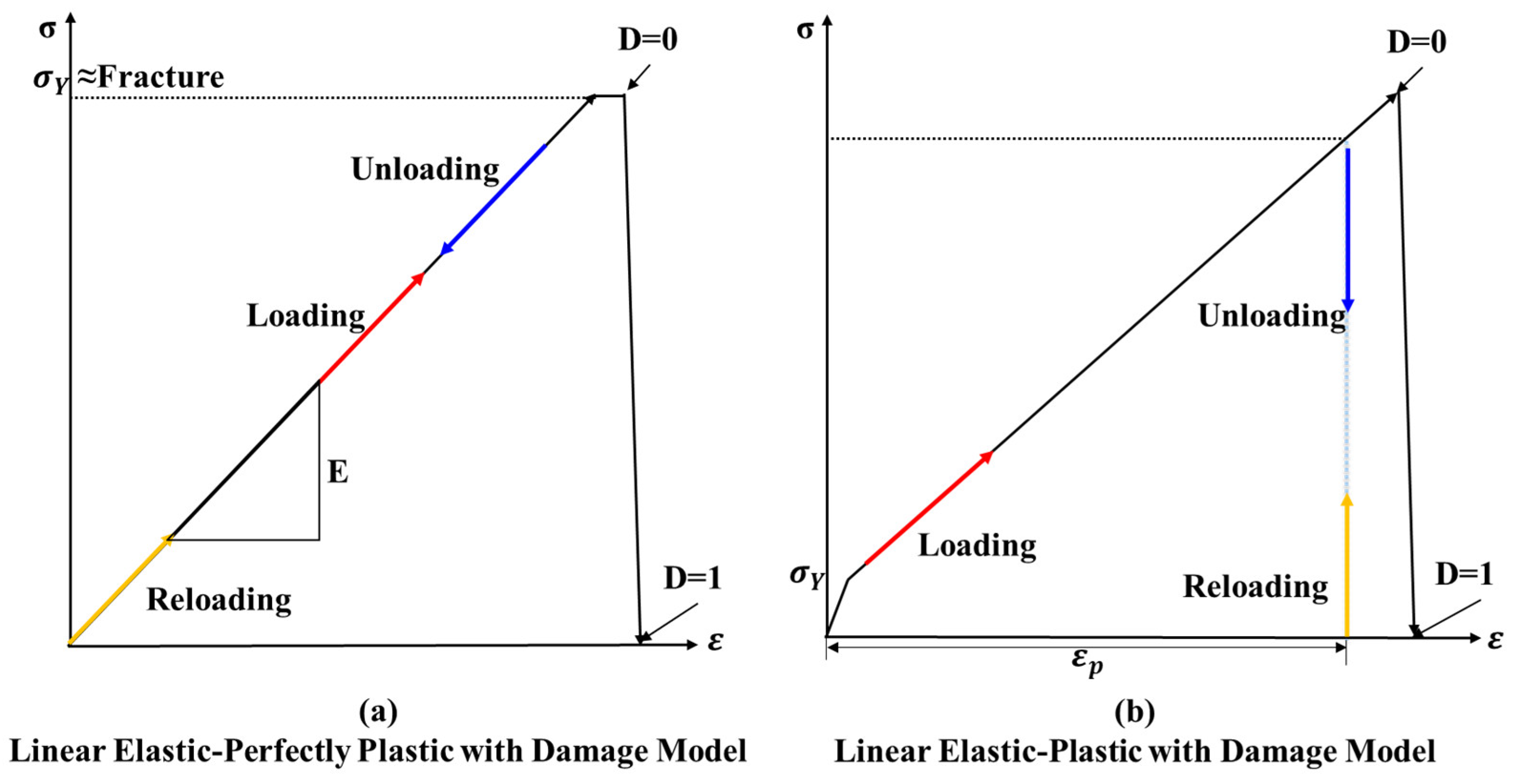
Figure 2.
Yield surface of crushable foam model with volumetric hardening.

Figure 3.
Yield surface and flow in the p–t plane assumed by linear Drucker-Prager model.
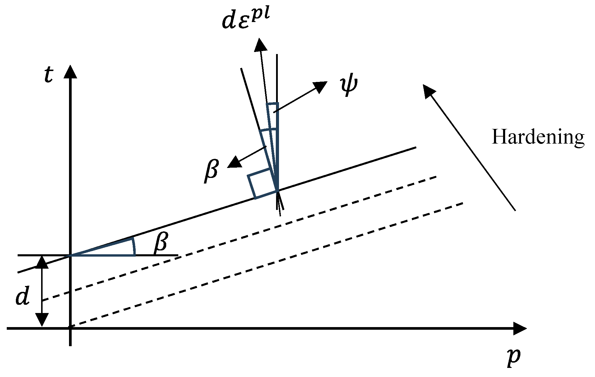
Figure 4.
Stress-strain curve with progressive damage degradation.
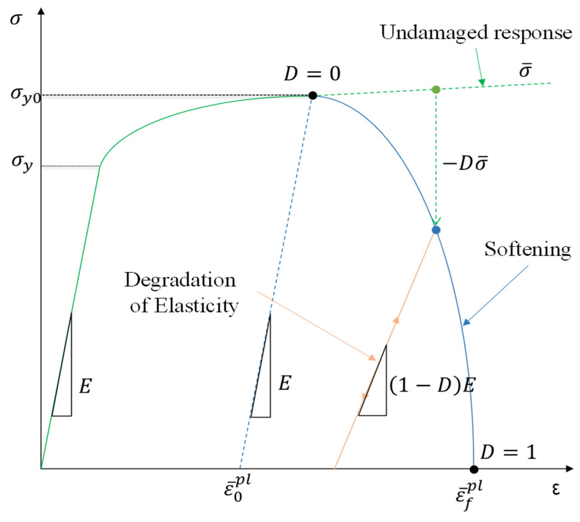
Figure 5.
Curve of compressive strength versus strain rate data (Tippmann, 2011).
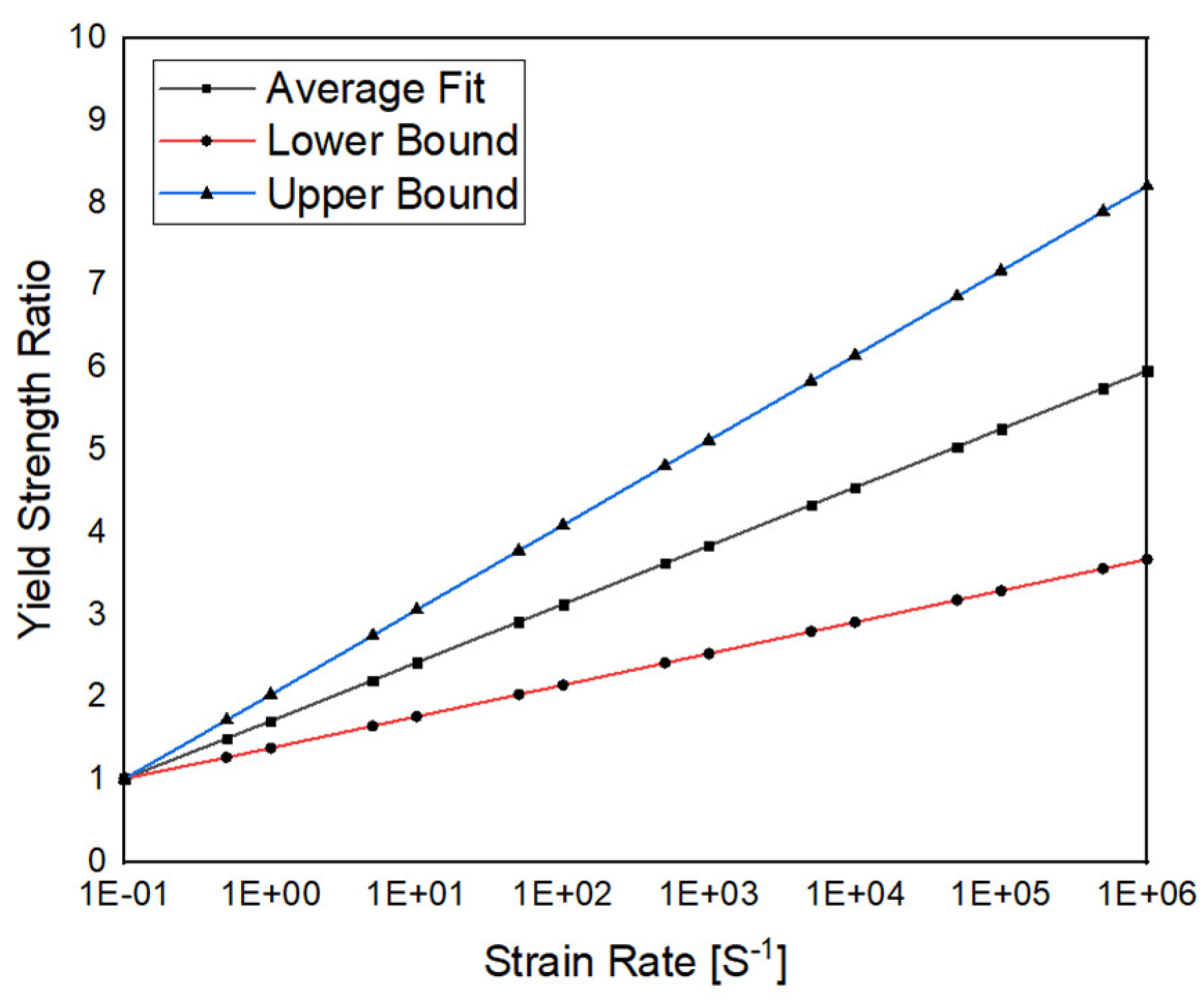
Figure 6.
Reaction forces and failure loads in the compression test.
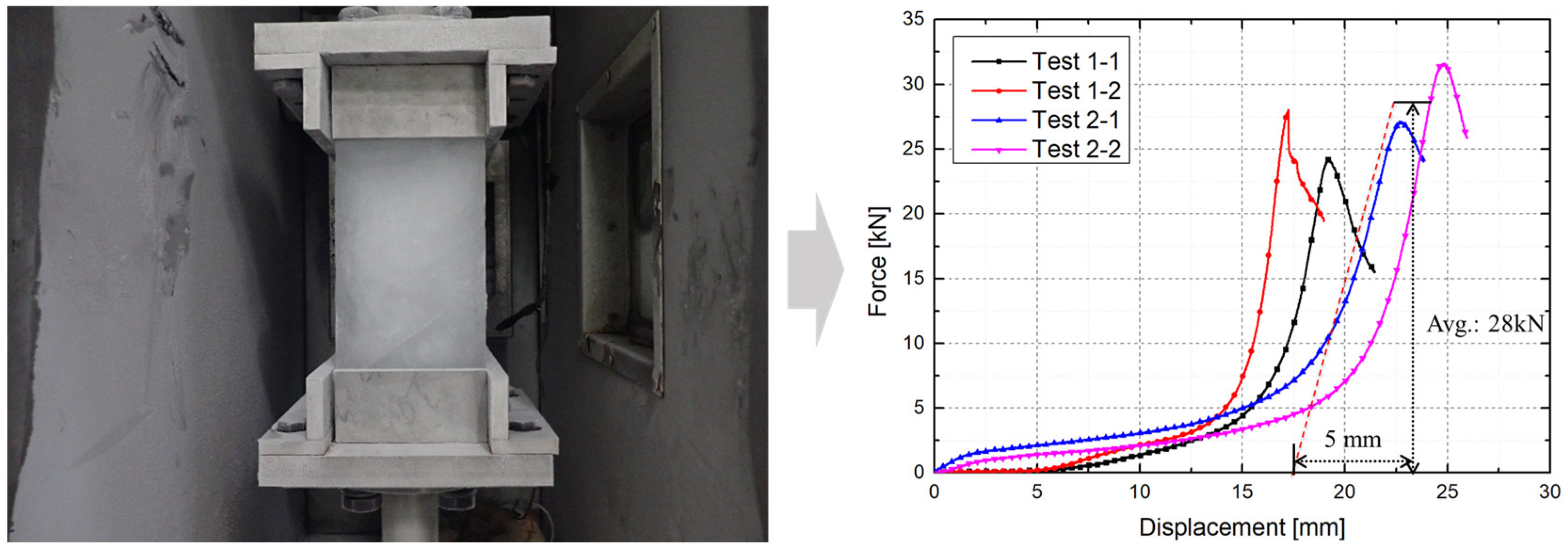
Figure 7.
Simulation model of ice compression test.
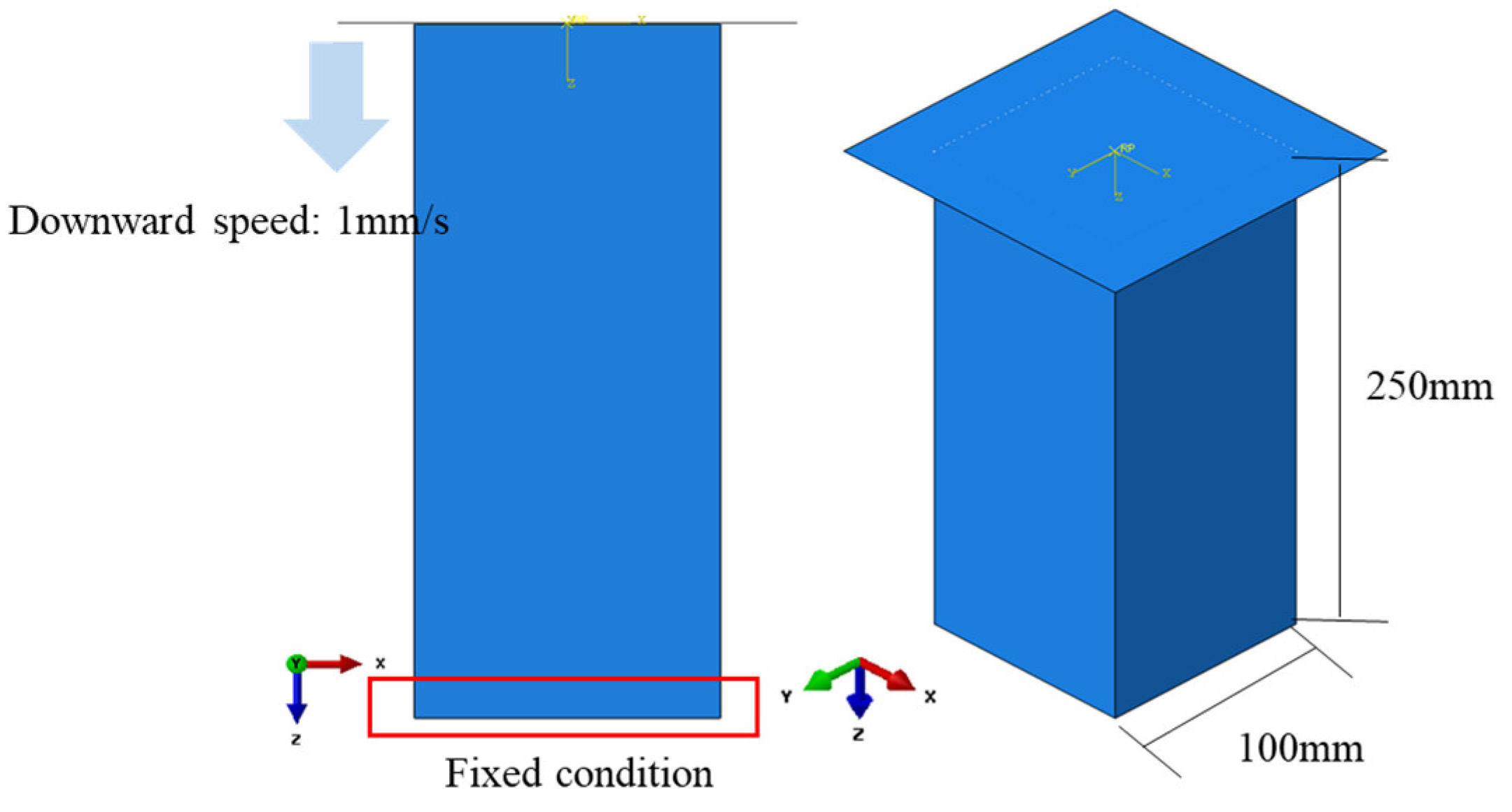
Figure 8.
Force vs. displacement simulated according to material models.

Figure 9.
Schematic configuration of ice collision (present study).
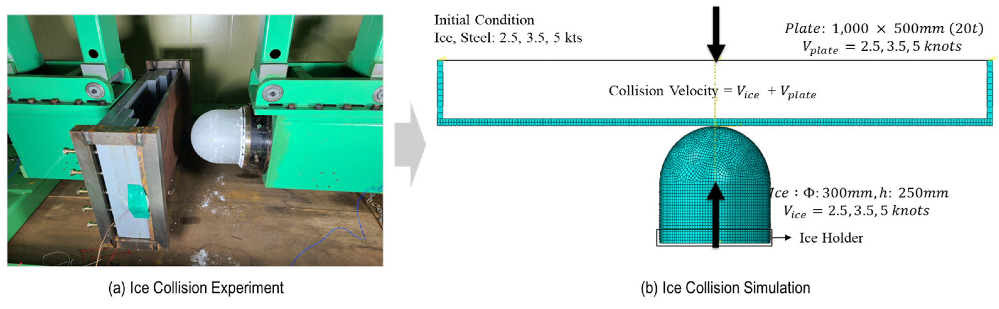
Figure 10.
Geometry of ice specimen and ice holder.
Figure 11.
Geometry of steel jig and steel plate jig.
Figure 12.
Simulation results of ice and steel after collision (10 kts).
Figure 13.
Simulation results of ice and steel after collision (10 kts).
Figure 14.
Simulation results of ice and steel after collision (10 kts).
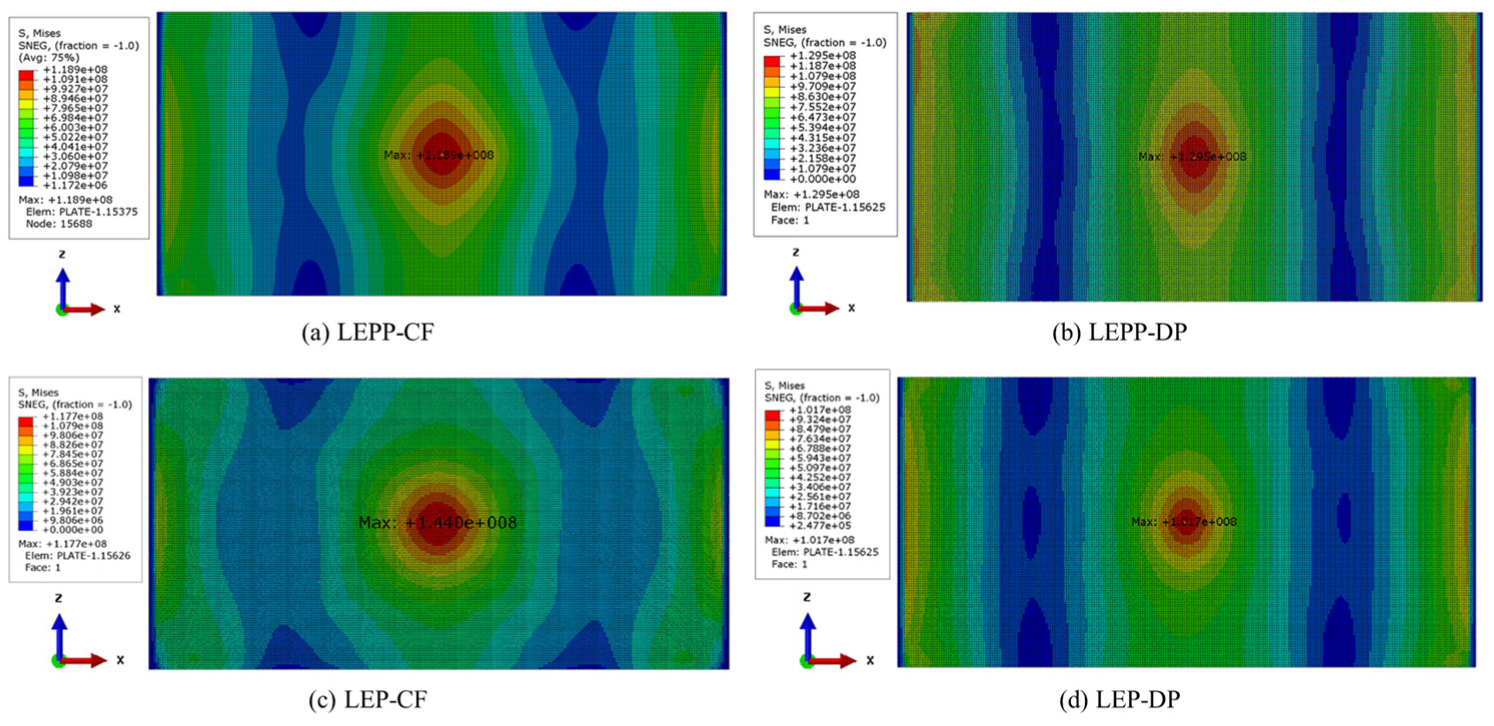
Figure 15.
History of according to ice material models.
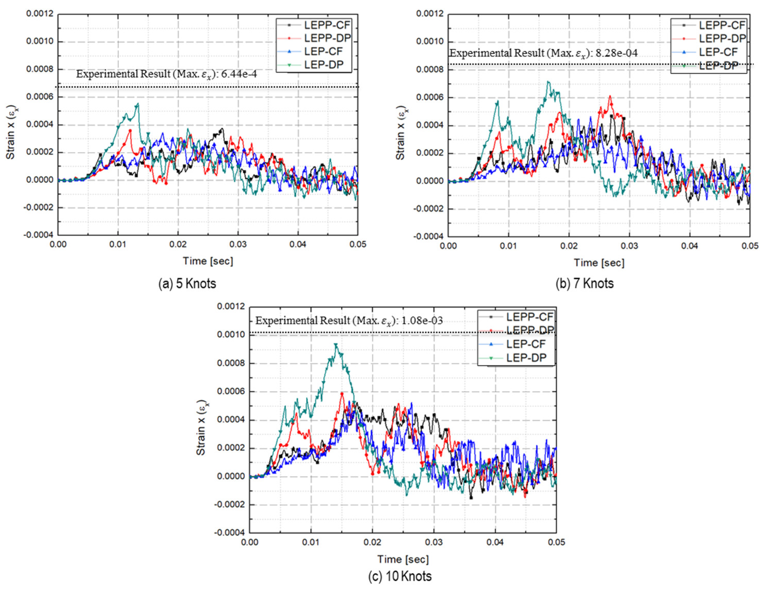
Figure 16.
History of according to the ice material models.
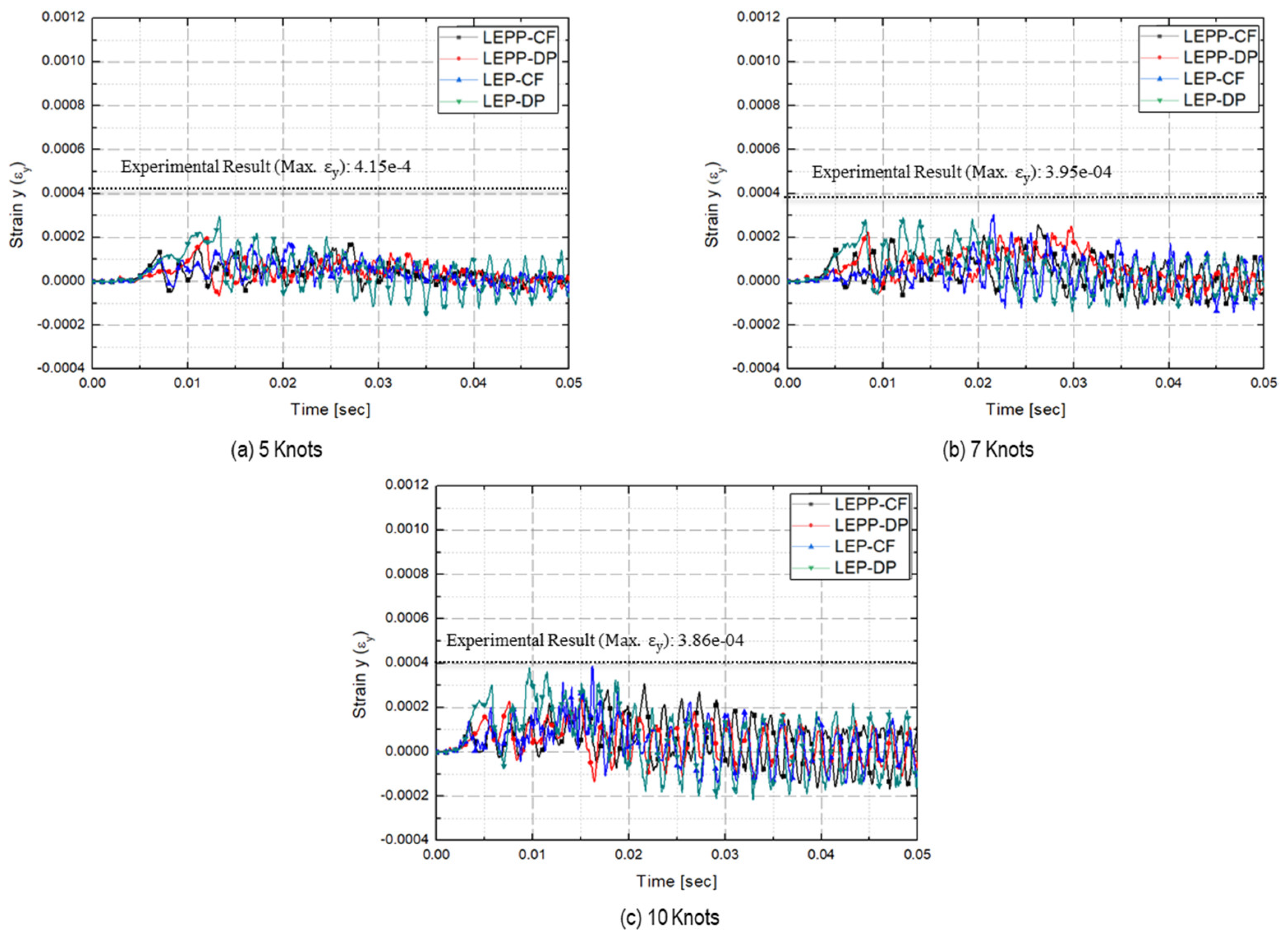
Figure 17.
Difference of maximum and according to the ice material models
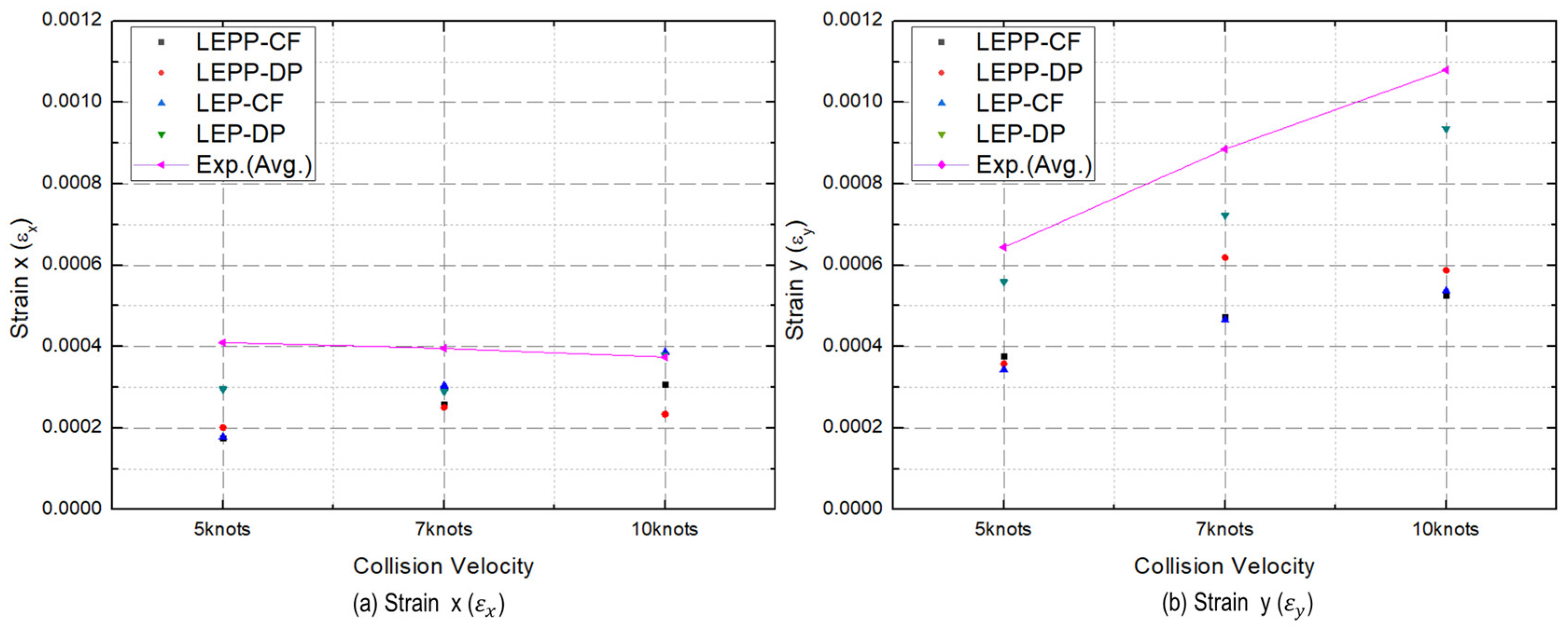
Figure 18.
History of collision force according to ice material models.
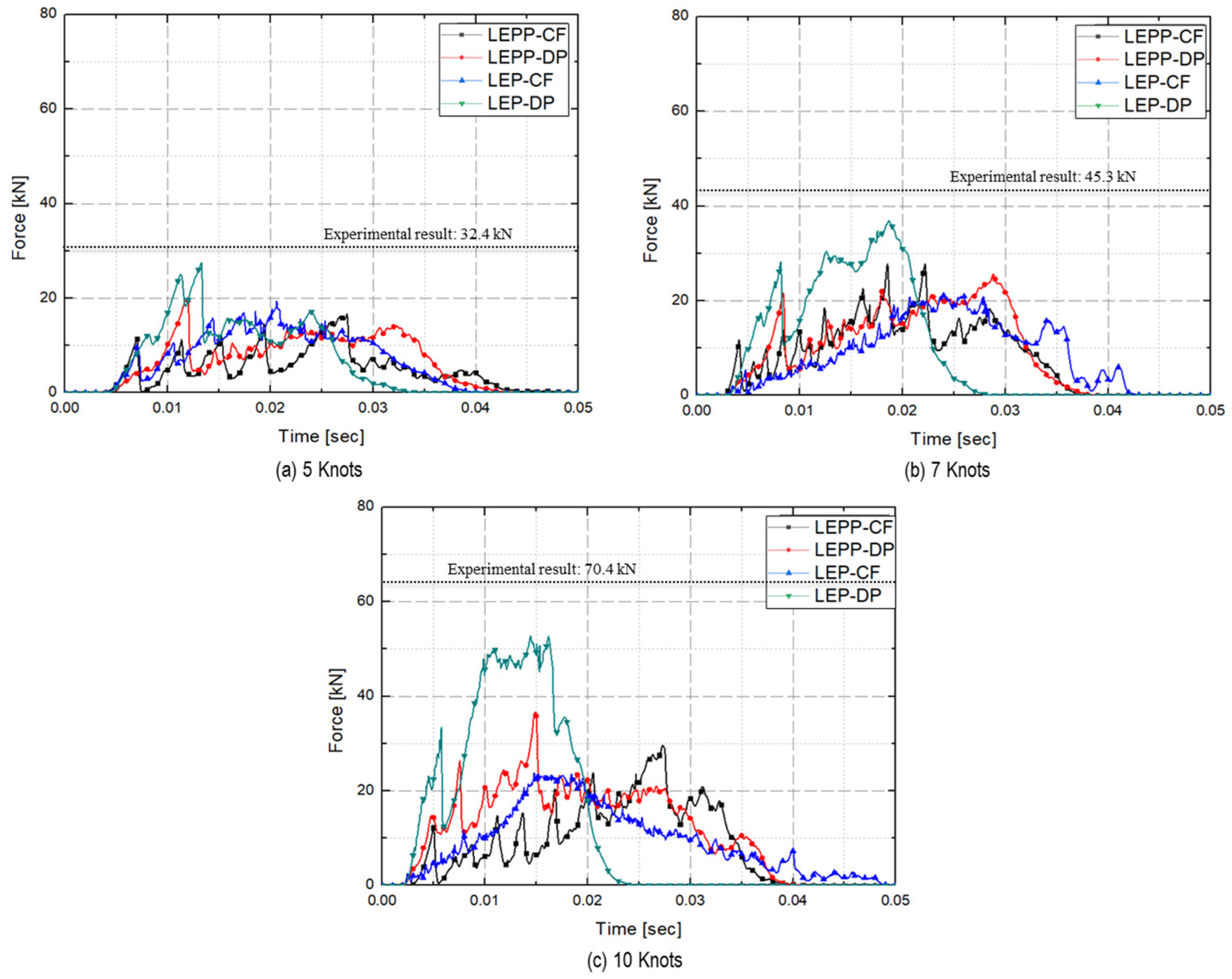
Figure 19.
Differences in maximum force according to the ice material models.
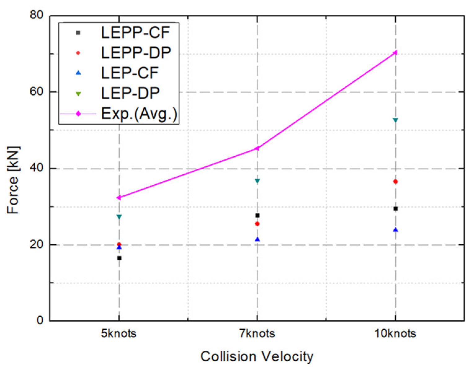
Figure 20.
Fractured shape of ice and steel after collision (10 kts).
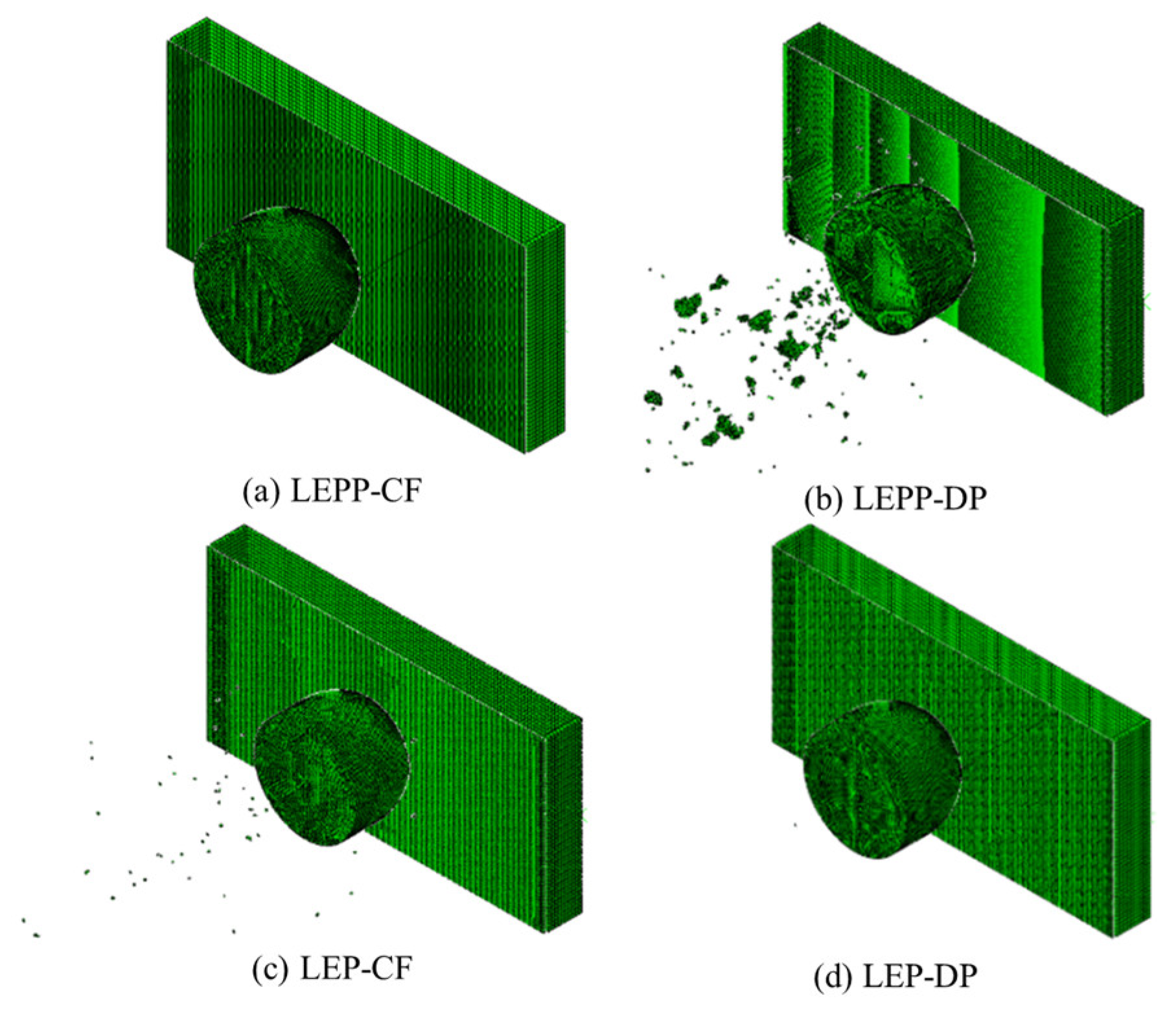
Figure 21.
Plastic strain distribution on the fractured ice surface (10 kts).
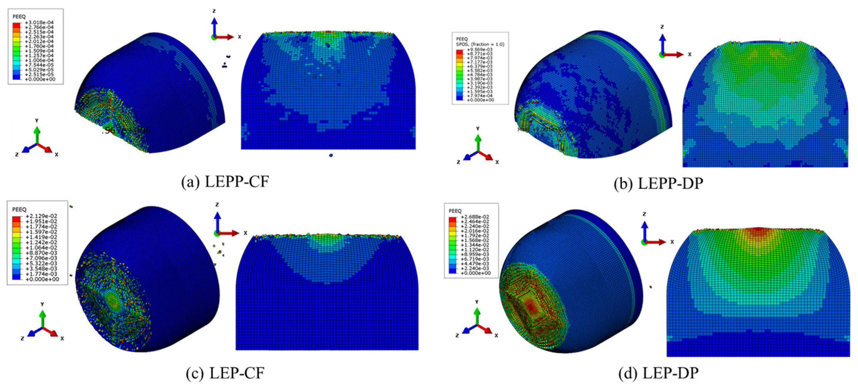
Figure 22.
Equivalent stress distribution on the steel after collision (10 kts).
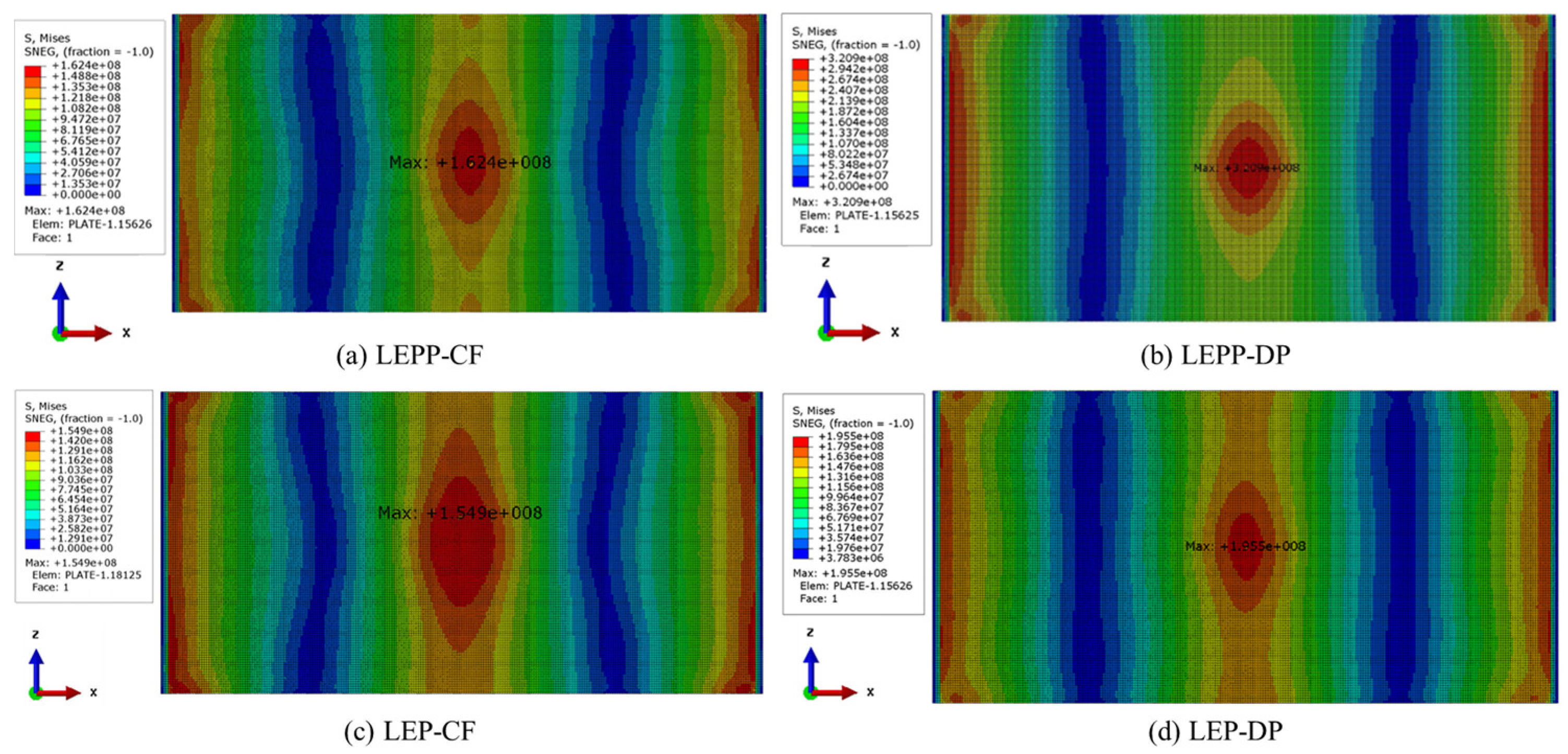
Figure 23.
History of according to the ice material models (with strain rate effect).
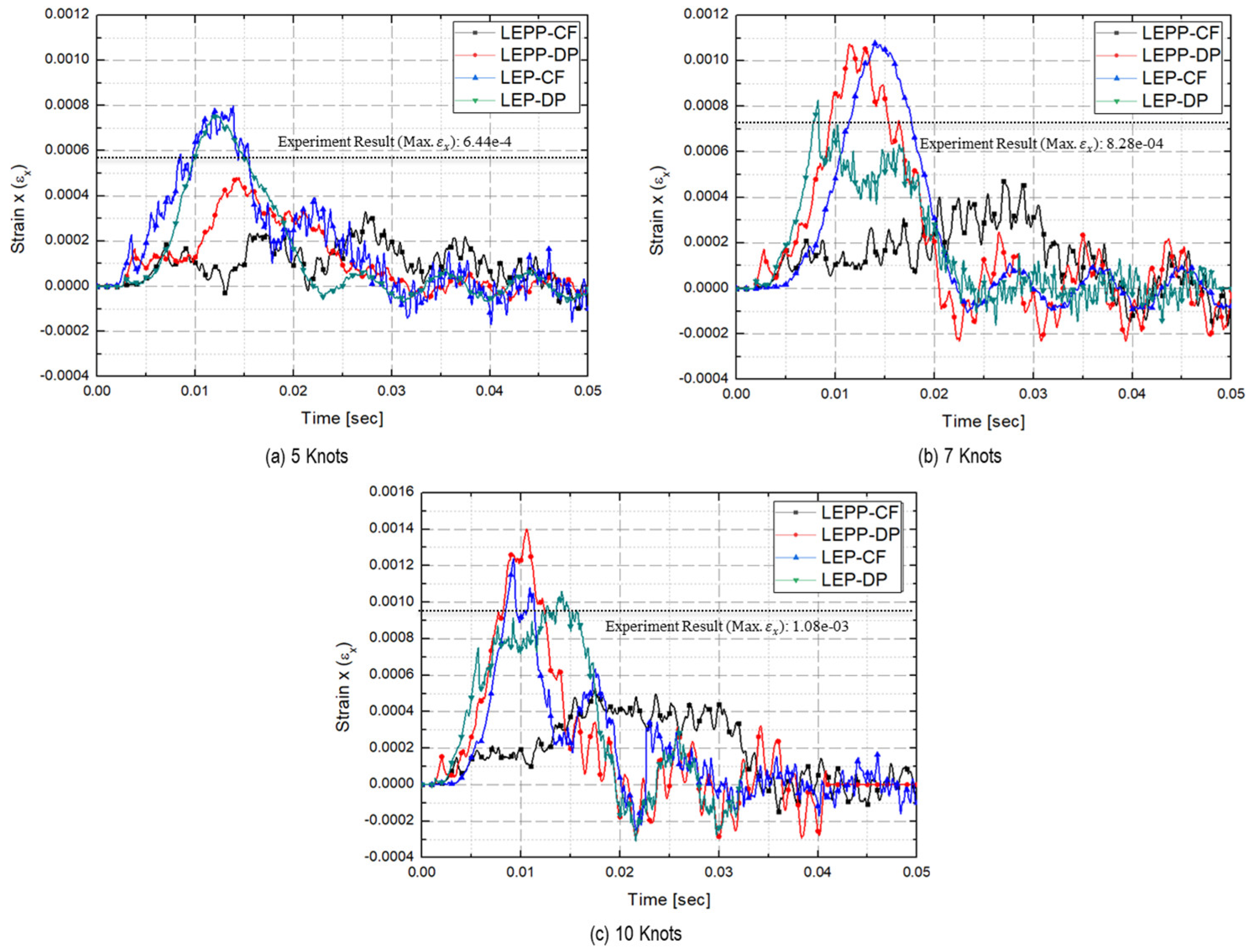
Figure 24.
History of according to the ice material models (with strain rate effect).
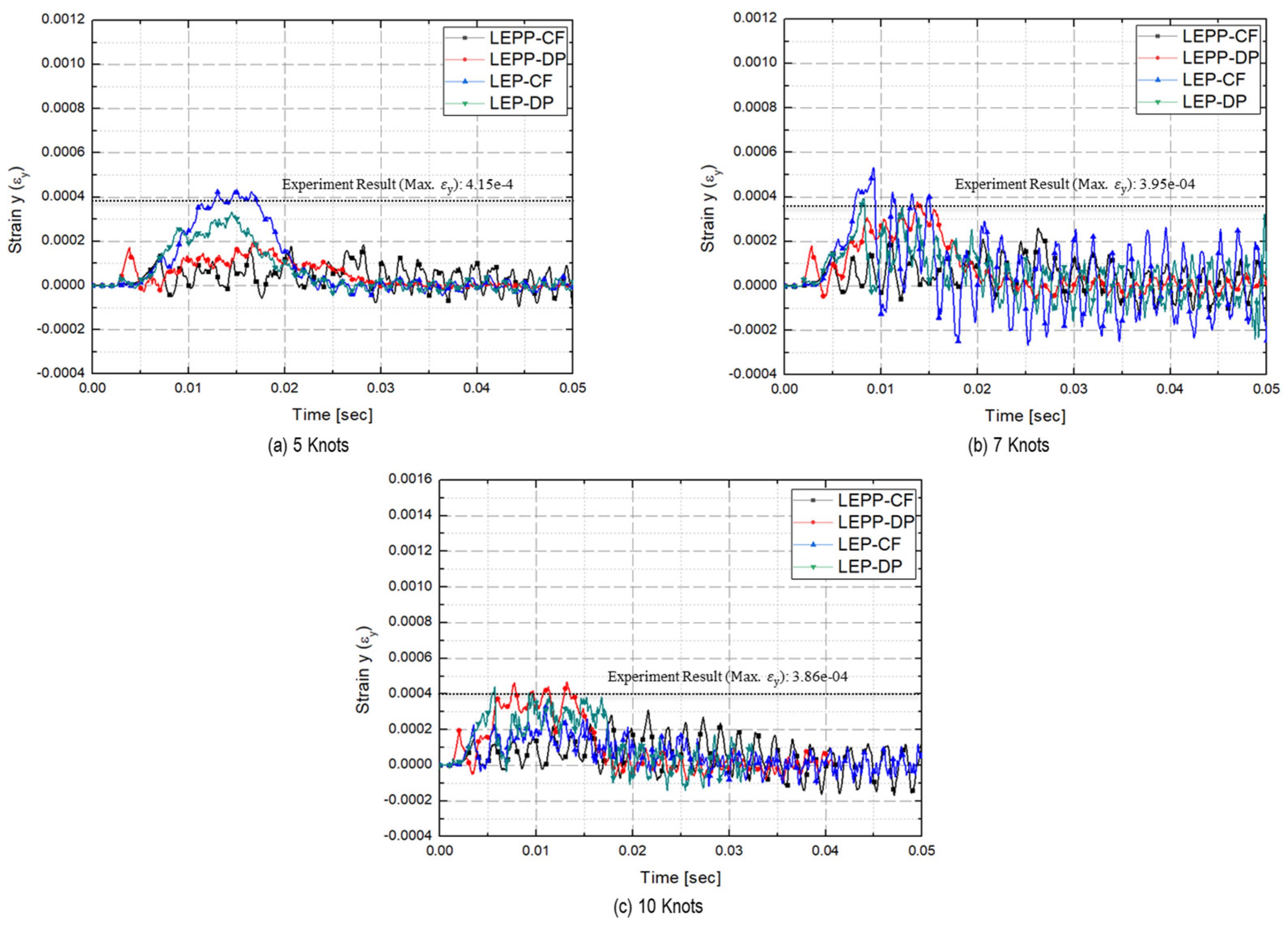
Figure 25.
Difference between the maximum and according to the ice material models (with strain rate effect).
Figure 25.
Difference between the maximum and according to the ice material models (with strain rate effect).
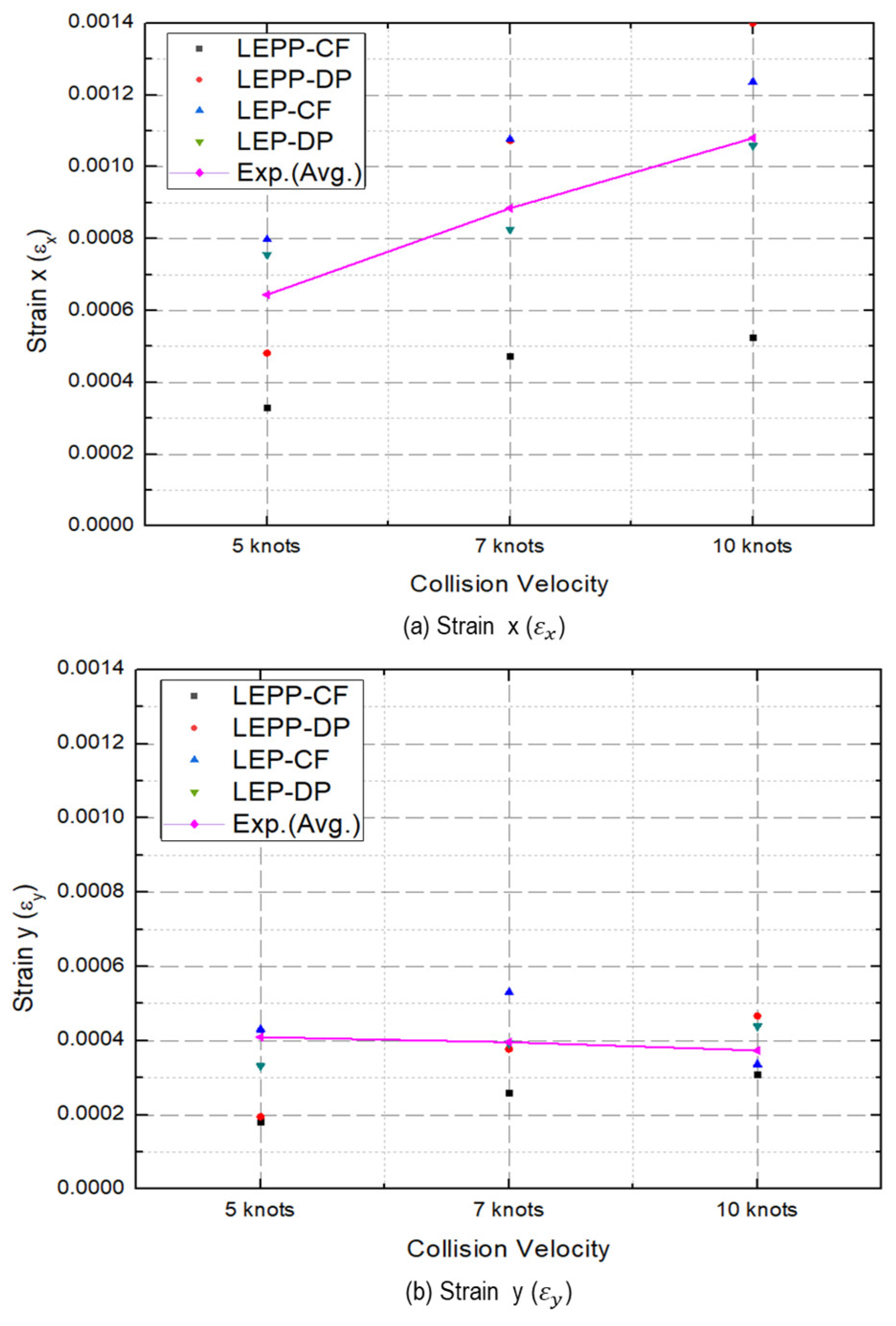
Figure 26.
History of collision force according to the ice material models (with strain rate effect).
Figure 26.
History of collision force according to the ice material models (with strain rate effect).
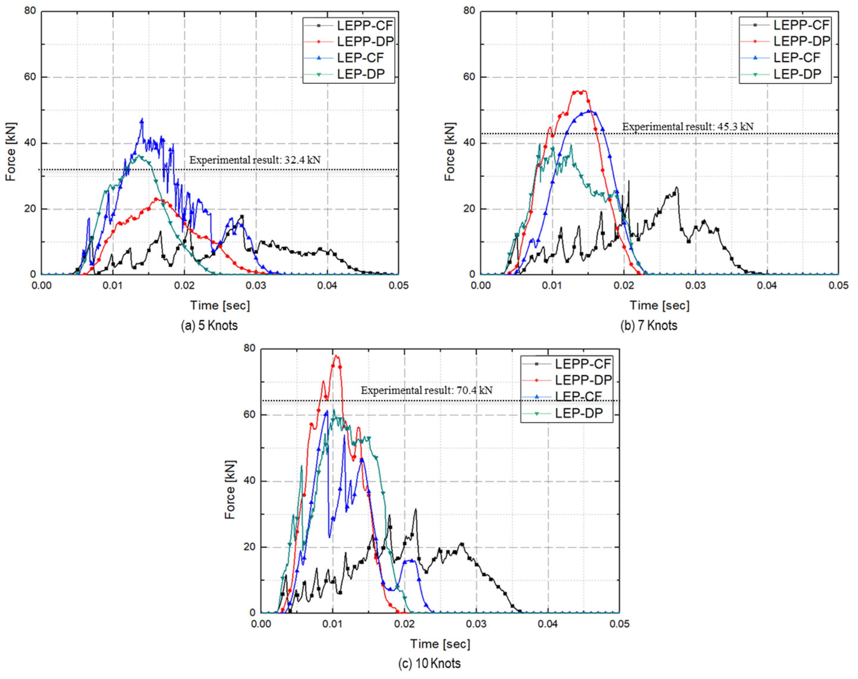
Figure 27.
Differences in maximum force according to the ice material models (with strain rate effect).
Figure 27.
Differences in maximum force according to the ice material models (with strain rate effect).
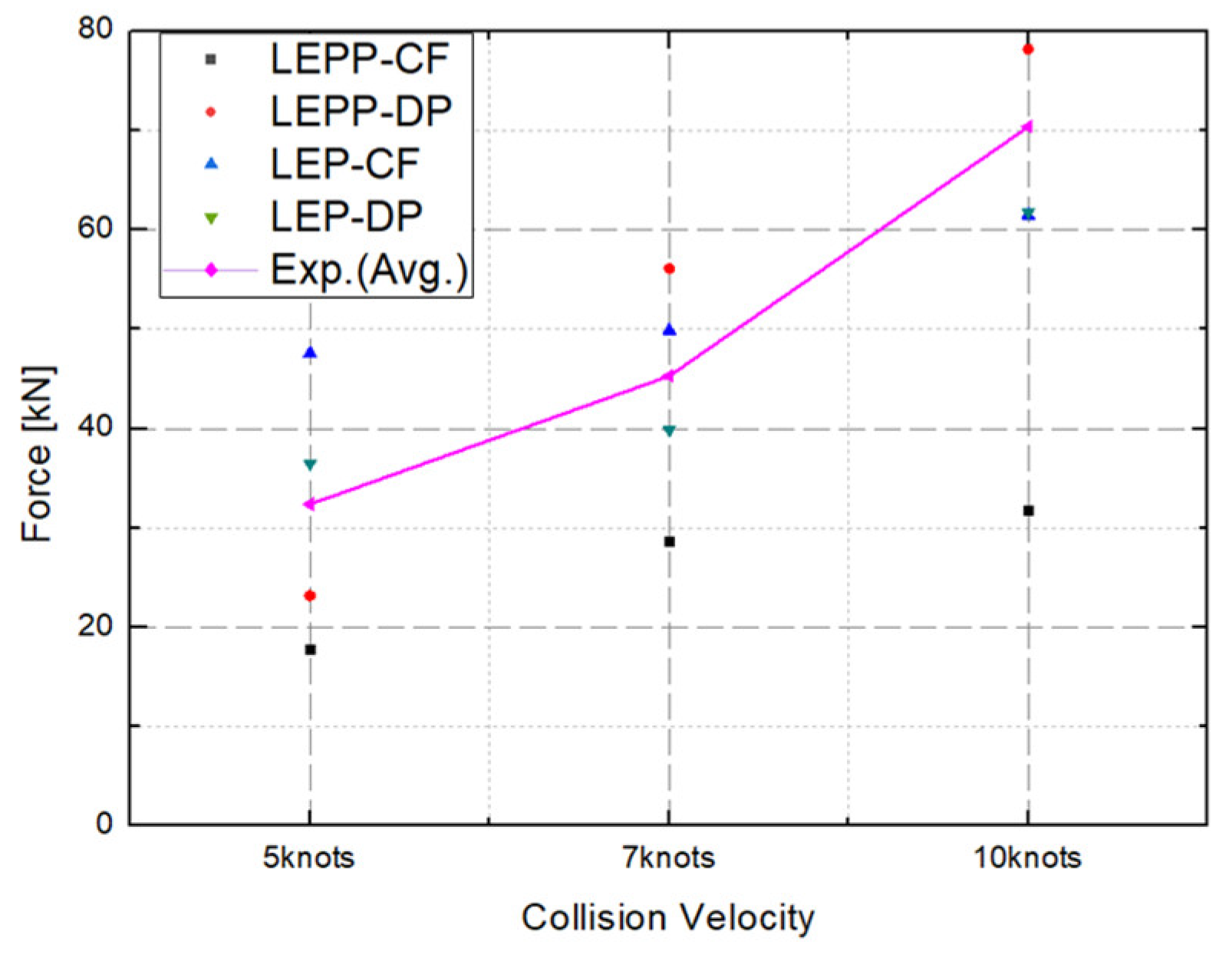
Figure 28.
Differences in maximum and according to the ice material case.
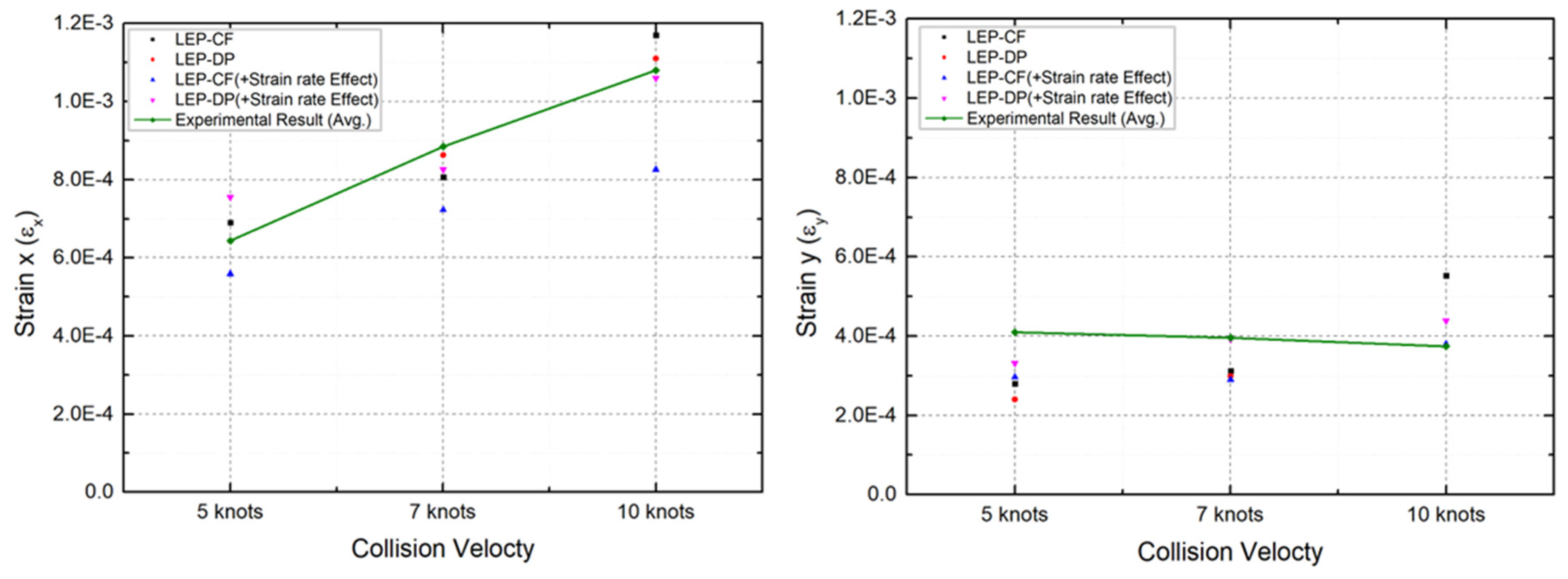
Figure 29.
Differences in maximum force according to the ice material case.
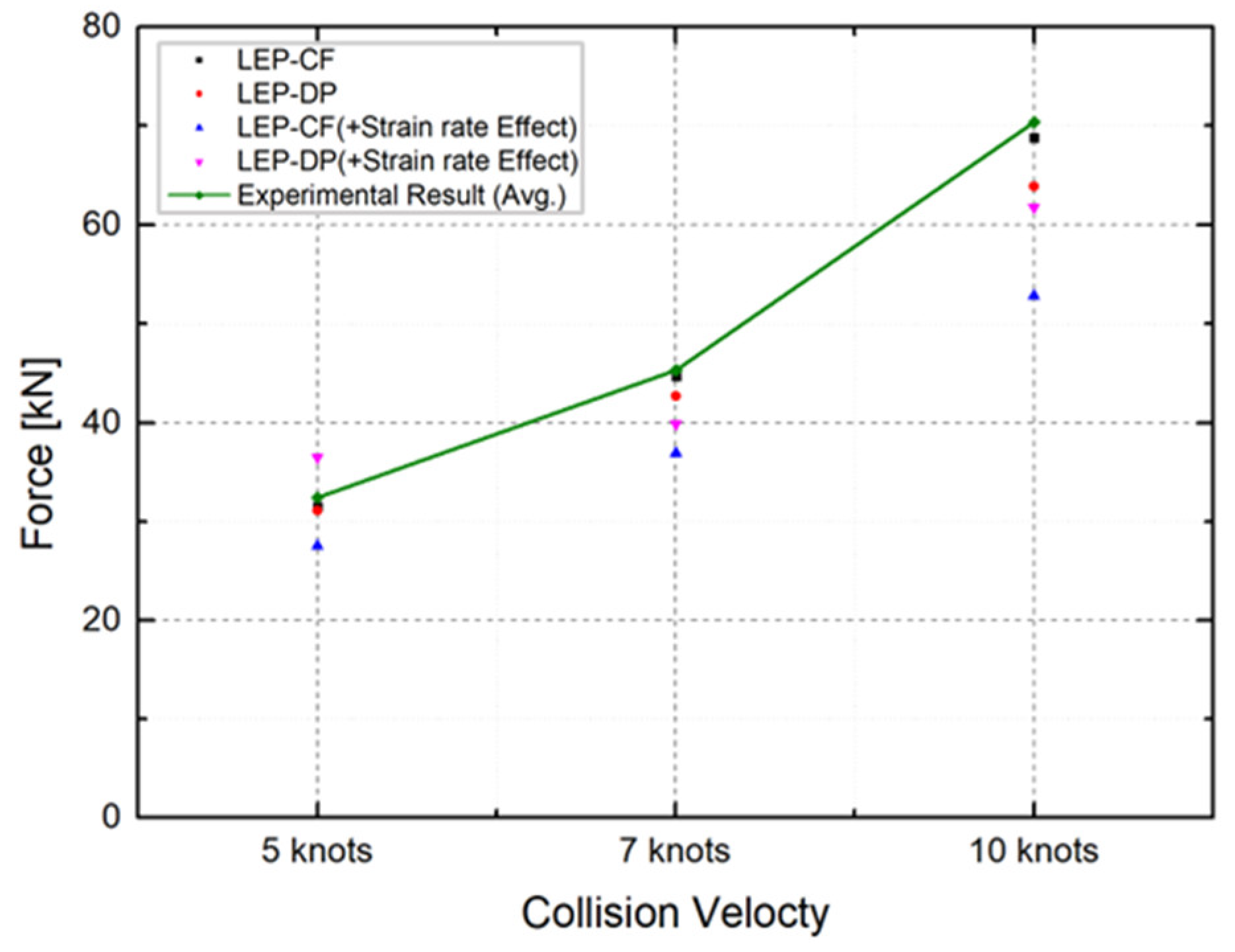
Table 1.
Yield criteria and yield ratio of ice materials.
| Material behavior |
Model | Equation | Reference |
|---|---|---|---|
| Yield criteria |
Crushable Foam |
|
Gagnon [3] Kim, et al. [4] |
| Drucker-Prager |
|
Kajaste-Rudnitski & Kujala [11] | |
| Damage model |
Ductile Damage |
|
Han, et al. [9] Kim, et al. [19] Jeon & Kim [20] |
| Strain rate dependency | - | Yield stress ratio as strain rate | Tippmann [24] |
Table 2.
Combination of material properties for numerical simulation.
| Material models |
Constitutive equation | Yield criterion | ||
|---|---|---|---|---|
| LEPP | LEP | CF | DP | |
| LEPP-CF | O | O | ||
| LEPP-DP | O | O | ||
| LEP-CF | O | O | ||
| LEP-DP | O | O | ||
Table 3.
Parameters of yield surface (LEPP model).
| LEPP | CF (Obisesan & Sriramula [23]) | DP (Jeon & Kim [20]) | |||
|---|---|---|---|---|---|
| Parameter | Compression Yield Stress Ratio | Hydrostatic Yield Stress Ratio | Friction Angle |
Flow Stress Ratio |
Dilation Angle |
| Value | 1.49 | 1.79 | 36 deg | 1 | 12 deg |
Table 4.
Hardening stress-strain (LEP model).
| LEP | Crushable Foam (CF) | Drucker Prager (DP) | ||
|---|---|---|---|---|
| Hardening Value |
Stress | Strain | Stress | Strain |
| 0.5 MPa | 0 | 0.5 MPa | 0 | |
| 3.3 MPa | 0.019 | 3 MPa | 0.025 | |
| 3.3 MPa | 0.5 | 3 MPa | 0.5 | |
Table 5.
Force and displacement simulated by material models.
| FEA Result | LEPP-CF | LEPP-DP | LEP-CF | LEPP-DP |
|---|---|---|---|---|
| Force [kN] | 28.2 | 27.9 | 27.8 | 28.2 |
| Displacement[mm] | 5.02 | 5.1 | 4.98 | 4.92 |
Table 6.
Summary of ice collision model (Present study).
| Ice Specimen | Ice Holder | Steel Plate | Steel Jig | ||
|---|---|---|---|---|---|
| Geometry |
= 300 mm = 250 mm |
= 300 mm = 50 mm |
1,000 × 500 mm Thickness= 20 mm |
1,000×500 mm 200×50×500mm |
|
| Element | Deformable Body | Rigid Body | Deformable Body | Rigid Body | |
| Shell Element (S4R) |
Rigid Element (R3D4) | Solid Element (C3D8R) |
Rigid Element (R3D4) | ||
| Contact | Hard contact with steel plate (penalty contact, frictionless) |
Tie condition with ice |
Hard contact with steel plate (penalty contact, frictionless) |
Tie condition with steel plate |
|
Table 7.
Comparison of maximum strain x () from experiment and FEA.
| Collision Velocity |
Experiment (Avg.) |
LEPP -CF | LEPP -DP | LEP -CF | LEP -DP |
|---|---|---|---|---|---|
| 5 kts | 6.44 × 10⁻⁴ | 3.77 × 10⁻⁴(41.4%) | 3.59 × 10⁻⁴(44.3%) | 3.44 × 10⁻⁴(46.7%) | 5.59 × 10⁻⁴(13.2%) |
| 7 kts | 8.85 × 10⁻⁴ | 4.72 × 10⁻⁴(46.6%) | 6.19 × 10⁻⁴(30.1%) | 4.65 × 10⁻⁴(47.4%) | 7.22 × 10⁻⁴(18.4%) |
| 10 kts | 1.08 × 10⁻³ | 5.26 × 10⁻⁴(51.3%) | 5.87 × 10⁻⁴(45.6%) | 5.37 × 10⁻⁴(50.3%) | 9.35 × 10⁻³(13.4%) |
| Difference | - | 46.4% | 40.0% | 51.3% | 15.0% |
Table 8.
Comparison of maximum strain y () from experiment and FEA.
| Collision Velocity |
Experiment (Avg.) |
LEPP -CF | LEPP -DP | LEP -CF | LEP -DP |
|---|---|---|---|---|---|
| 5 kts | 4.10 × 10⁻⁴ | 1.76 × 10⁻⁴(57.1%) | 2.01 × 10⁻⁴(50.9%) | 1.78 × 10⁻⁴(56.5%) | 2.96 × 10⁻⁴(27.9%) |
| 7 kts | 3.96 × 10⁻⁴ | 2.58 × 10⁻⁴(34.9%) | 2.51 × 10⁻⁴(36.6%) | 1.81 × 10⁻⁴(23.1%) | 2.90 × 10⁻⁴(26.8%) |
| 10 kts | 3.74 × 10⁻⁴ | 3.09 × 10⁻⁴(17.3%) | 2.34 × 10⁻⁴(37.4%) | 3.87 × 10⁻⁴(-3.4%) | 3.80 × 10⁻⁴(-1.5%) |
| Difference | - | 46.4% | 40.0% | 51.3% | 15.0% |
Table 9.
Comparison of maximum force from experiment and FEA.
| Collision Velocity |
Experiment (Avg.) |
LEPP -CF | LEPP -DP | LEP -CF | LEP -DP |
|---|---|---|---|---|---|
| 5 kts | 32.4 | 16.7(48.6%) | 20.1(37.9%) | 19.3(40.3%) | 27.5(15.1%) |
| 7 kts | 45.3 | 31.8(38.6%) | 25.6(43.6%) | 21.4(52.8%) | 36.9(18.5%) |
| 10 kts | 70.4 | 24.99(58.0) | 36.6(48.0%) | 23.9(66.1%) | 52.8(25.0%) |
| Difference | - | 48.4% | 43.1% | 53.1% | 22.1% |
Table 10.
Comparison of maximum strain x () between the experiment and FEA (with strain rate effect).
Table 10.
Comparison of maximum strain x () between the experiment and FEA (with strain rate effect).
| Collision Velocity |
Experiment (Avg.) |
LEPP -CF | LEPP -DP | LEP -CF | LEP -DP |
|---|---|---|---|---|---|
| 5 kts | 6.44 × 10⁻⁴ | 3.30 × 10⁻⁴(48.8%) | 4.82 × 10⁻⁴(25.2%) | 7.98 × 10⁻⁴(-23.9%) | 7.55 × 10⁻⁴(-17.3%) |
| 7 kts | 8.85 × 10⁻⁴ | 4.72 × 10⁻⁴(46.6%) | 1.07 × 10⁻³(-21.3%) | 1.08 × 10⁻³(-21.7%) | 8.26 × 10⁻⁴(6.7%) |
| 10 kts | 1.08 × 10⁻³ | 5.26 × 10⁻⁴(51.3%) | 1.73 × 10⁻³(-29.6%) | 1.24 × 10⁻³(-14.5%) | 1.06 × 10⁻³(2.0%) |
| Difference | - | 48.9% | 30.2% | 20.0% | 8.7% |
Table 11.
Comparison of maximum strain y () between the experiment and FEA (with strain rate effect).
Table 11.
Comparison of maximum strain y () between the experiment and FEA (with strain rate effect).
| Collision Velocity |
Experiment (Avg.) |
LEPP -CF | LEPP -DP | LEP -CF | LEP -DP |
|---|---|---|---|---|---|
| 5 kts | 4.10e-04 | 1.83 × 10⁻⁴(55.4%) | 1.95 × 10⁻⁴(52.4%) | 4.31 × 10⁻⁴(-5.03%) | 3.32 × 10⁻⁴(19.0%) |
| 7 kts | 3.96e-04 | 2.59 × 10⁻⁴(34.6%) | 3.78 × 10⁻⁴(4.6%) | 5.30 × 10⁻⁴(-33.9%) | 3.92 × 10⁻⁴(0.9%) |
| 10 kts | 3.74e-04 | 3.09 × 10⁻⁴(17.4%) | 4.67 × 10⁻⁴(-24.8%) | 3.36 × 10⁻⁴(10.0%) | 4.39 × 10⁻⁴(-17.4%) |
| Difference | - | 35.8% | 27.3% | 16.3% | 12.4% |
Table 12.
Comparison between the experimental and FEA-derived maximum force (with strain rate effect).
Table 12.
Comparison between the experimental and FEA-derived maximum force (with strain rate effect).
| Collision Velocity |
Experiment (Avg.) |
LEPP -CF | LEPP -DP | LEP -CF | LEP -DP |
|---|---|---|---|---|---|
| 5 kts | 32.4 | 17.8 (45.1%) | 23.2 (28.5%) | 47.6 (-46.8%) | 36.5 (-12.7%) |
| 7 kts | 45.3 | 28.7 (36.7%) | 56.1 (-23.8%) | 49.9 (-10.1%) | 39.9 (11.8%) |
| 10 kts | 70.4 | 31.8 (54.9%) | 78.2 (-11.0%) | 61.5 (12.6%) | 61.8 (12.2%) |
| Difference | - | 45.6% | 21.1% | 34.8% | 12.2% |
Disclaimer/Publisher’s Note: The statements, opinions and data contained in all publications are solely those of the individual author(s) and contributor(s) and not of MDPI and/or the editor(s). MDPI and/or the editor(s) disclaim responsibility for any injury to people or property resulting from any ideas, methods, instructions or products referred to in the content. |
© 2023 by the authors. Licensee MDPI, Basel, Switzerland. This article is an open access article distributed under the terms and conditions of the Creative Commons Attribution (CC BY) license (http://creativecommons.org/licenses/by/4.0/).
Copyright: This open access article is published under a Creative Commons CC BY 4.0 license, which permit the free download, distribution, and reuse, provided that the author and preprint are cited in any reuse.


