Submitted:
17 November 2023
Posted:
20 November 2023
Read the latest preprint version here
Abstract
Accurately estimating the State-of-Health (SOH) of lithium-ion batteries is of great importance within the field of battery management systems. Some new technique is now being developed to ensure the secure operation of lithium-ion batteries. The model being suggested in this study employs a deep learning framework that integrates discretized input data. This study utilized two distinct neural network architectures, including a standard fully connected neural network (FCNN) and a bidirectional long short-term memory (LSTM) architecture. The process of converting digitized feature values into binary bits enables the storing of inferred values within a Lookup Table (LUT-Memory). The efficiency and speed of the inference process are expected to improve when inferring a pre-trained deep neural network architecture directly. The primary objective of this study is to accurately build a lookup table that efficiently correlates the state of health (SOH) of lithium-ion batteries, while ensuring a tolerable degree of imprecision. The findings derived from the lithium-ion battery dataset provided by NASA PCoE provide evidence to support the claim that the suggested methodology exhibits similar performance to complete models that require inference during testing. The error assessment metrics, namely Root Mean Square Error (RMSE), Mean Absolute Error (MAE), and Mean Absolute Percentage Error (MAPE), have been employed for quantitative analysis of the accuracy of status of health (SOH) prediction. The aforementioned indicators exhibit a notable level of precision in forecasting the State of Health (SOH).
Keywords:
Lithium-Ion Batteries
; SoH
; SoC
; RUL
; Batteries
; Deep Learning
; LUT
1. Introduction
The use of lithium-ion batteries has rapidly increased due to their low-cost, high-energy densities, low self-discharge rate, and long lifetime compared to other batteries [1,2,3,4]. Hence, lithium-ion batteries have gained significant prominence across diverse domains, including but not limited to mobile computing devices, aerospace applications, electric cars, and energy storage systems [5,6]. Despite the noteworthy advantages of lithium-ion batteries, a significant drawback is the occurrence of capacity fading upon repeated utilization. In addition, it is imperative to diligently observe and precisely assess the capacity, since an inaccurate evaluation of capacity might result in irreversible harm to the battery through excessive charging or discharging [7]. The assessment of battery capacity fade relies heavily on, what is called, the state of health or SOH, which serves as a pivotal indication. Hence, it is vital to precisely determine the State of Health (SOH) of lithium-ion batteries in order to ensure their safety and dependability [8].
Numerous research endeavors have been undertaken to get a precise assessment of the state of health (SOH). In general, the studies can be categorized into three distinct groups: model-based methods [9,10,11,12,13,14], data-driven methods [15,16], and hybrid methods [17,18].
The evaluation of battery health state, as determined by the State of Health (SOH) metric, was conducted based on the varying beginning capacities of each battery. There exist several approaches for determining the state of health (SOH) of a battery. However, the predominant methods revolve around assessing the impedance and its useful capacity. The utilization of the battery's impedance as a measuring technique is deemed unsuitable for online applications due to the necessity of specialized instruments, for example the electrochemical-impedance-spectroscopy. Hence, most studies employed the State of Health (SOH) metric of a battery, which was determined by its usable capacity.
1.1. Model-based Methods
Battery State of Health (SOH) estimation can be achieved by a number of model-based approaches, which entail building a model of a battery and including the internal deterioration process inside the model. Knowledge of the internal battery reaction mechanisms, the accurate formulation of the mathematical equations driving these reactions, and the development of effective simulation models are all essential for model-based approaches. There may be difficulties in putting these ideas into practice.
Lithium-ion battery life was predicted using a weighted ampere-hour throughput model in a study by Onori et al. [19]. The researcher determined how severely the batteries had been damaged. To determine a battery's SoH, Plett [20] applied an analog circuit model and an improved Kalman filter. To determine a battery's SoH, Goebel et al. [21] relied on nominal filtering methods. They discovered that battery capacity is proportional to the square of the internal impedance.
Wang et al. [22] presented a method for estimating a battery's SoH, or state of health. This method takes battery discharge rates as input variables into a state-space model. The SOH of a battery was predicted using a single-particle model developed by Li et al. [23] that is grounded on the physics of electrolytes. The degeneration of the internal mechanisms and the batteries were the focus of this investigation. From a chemical perspective
The construction of a precise aging model for lithium-ion batteries is difficult due to the complex structure of the chemical interactions occurring within the battery, although model-based approaches are useful in forecasting the state of health (SOH) of batteries.
Furthermore, various environmental variables, such as operational temperature, anode and cathode materials, and related parameters, have a major impact on the performance of lithium-ion batteries. Therefore, there are difficulties in establishing a reliable aging model for lithium-ion batteries.
1.2. Data-driven Methods
Improvements in hardware have allowed computers to do increasingly complex mathematical operations in recent years. Concurrently, there has been an uptick in the number of databases that can be mined for information on a person's State of Health (SOH) thanks to the growing use of data-driven methodologies for this purpose. This paved the way for the broad adoption of data-driven approaches.
Even without a thorough understanding of the battery's internal structure and aging mechanisms from an electrochemical standpoint, a data-driven method allows for reliable prediction of the battery's State of Health (SOH). Therefore, these methods can be implemented with little to no familiarity with a battery's electrochemical properties or the environmental context. The success of data-driven approaches relies greatly on the accuracy and usefulness of the information that is collected. Acquiring attributes that are highly linked with the degradation process is crucial to the success of a data-driven model.
Hu et al. [24] suggested using sparse Bayesian predictive modeling with a sample entropy metric to boost the reliability of voltage sequence predictions. The SOH of a battery can be estimated and analyzed with the help of a hidden Markov model, which was introduced by Piao et al. [25]. Liu et al. [26] used Gaussian process regression to estimate health status in their investigation. This method combines covariance and mean functions into a single estimate.
Khumprom and Yodo [27] presented a data-driven prognosis method that makes use of deep neural networks to foretell the SoH and RUL of lithium-ion batteries. Xia and Abu Qahouq [28] developed a method for adaptive SOH estimate based on an online alternating current (AC) complex impedance and a feedforward neural network (FNN). The use of recurrent neural networks to foresee battery performance decline has been demonstrated by Eddahech et al. [29]. Shen et al. [30] proposed using a deep convolutional neural network (CNN) trained on recorded current and voltage to estimate battery capacity.
In this work, we develop an efficient processing method to replace the inference operation through the trained network with a pre calculated LUT memory. The accuracy and efficiency of SOH estimation by using this substitute proved to be acceptable. This method is completely non-using the different machine learning models trained, but solely relies on the quantization operation and chosen bits per feature.
2. Dataset Description
The information utilized in this work for the purpose of estimating the lithium-ion batteries State of Health (SOH) was acquired from the NASA Prognostics Center [31]. The four batteries used, indicated as #5, #6, #7, and #18, which have been extensively utilized for the purpose of State of Health (SOH) estimate [32,33,34]. The dataset utilized in this study comprised operational profiles and impedance measurements of 18,650 lithium-ion batteries measurement trials throughout the processes of charging and discharging at ambient temperature (around 24C). The batteries underwent a charging process where a 1.50 A current was maintained in a continuous flow until the voltage reached 4.2 V. Subsequently, the charging proceeded at 4.2 V of constant voltage until the current decreased to a value below 20 mA. Battery numbers 5, 6, 7, and 18 were discharged at a constant current of 2 A until their voltages hit 2.7 V for B0005, 2.5 V for B0006, 2.2 V for B0007, and 2.5 V for B0018 batteries. This process took place until the batteries' individual voltages reached the desired levels. Eventually, the batteries gradually start to decrease in capacity as the number of charging and discharging continues to grow. It is taken that, once the battery dropped 30% from the rated capacity, its end-of-life (EOL) is reached, nominally from 1.4Ah to 2.0 Ah.
The aforementioned collected datasets provide the capability to predict the batteries SoH. The battery's aging process is correlated with the number of cycles, as seen in Figure 1. Additionally, Table 1 illustrates the features value boundaries observed throughout an aging cycle for battery #5.
The primary indication of battery deterioration is the decline in capacity, which is mostly associated with the state of health SOH. The definition of SOH is determined by its capacity, which may be calculated easily using the next formula. In this formula, Cusable and Crated denote the actual and notional capabilities, correspondingly. This study we utilize lithium-ion battery time series data for the purpose of predicting State of Health (SOH). The research also delves into the essential process of data preprocessing in order to ensure accurate and reliable predictions.
To illustrate more, the term "Cusable" refers to the usable capacity of a device, representing the maximum amount of capacity that may be released when it is entirely discharged. On the other hand, "Crated" denotes the rated capacity, which is the capacity value supplied by the manufacturer. The available capacity diminishes as time progresses.
Data Preprocessing
The seven extracted, namely, battery capacity, voltage, current, temperature, charging voltage, charging current, Instant of time (from the start of the download), are subjected to normalization. Thise time-based characteristic is then prepared, and the feature data has been divided into two datasets, one for training and the others for testing. During the stage of model training, the dataset employed for training was partitioned into two parts, namely the training data and the validation data. Following that, the models were subjected to training utilizing the Feedforward Neural Networks (FFNNs) model and the Long Short-Term Memory (LSTM) model. The hyperparameters of the architecture were fine-tuned during the training process in order to achieve satisfactory performance. During the stage of performance evaluation, the trained model underwent testing using the test dataset, and the evaluation of its performance was conducted using metrics like the mean absolute percentage error, the mean absolute error, and mean squared error, MAPE, MAE, MSE, respectively.
Firstly, the data undergo a filtering process wherein outliers and missing values are eliminated using techniques like moving averages or intermediate values. This process is essential as it helps to reveal the periodic deterioration patterns exhibited by the battery data. By eliminating outlier values, the potential for misleading or confounding the model is minimized. Additionally, periodic averaging of the data helps to mitigate short-term oscillations, further enhancing the reliability and stability of the dataset.
Data normalization is a widely utilized technique in depth modeling methods, as it is seen suitable for enhancing both the convergence of the model and the accuracy of the prediction. Normalization will be conducted using the minimum-maximum approach, which involves scaling the data within the range of 0 to 1. The aforementioned relationship is mathematically represented by the following equation. In the given context, the symbol "xn" is used to denote the processed data, while "x" represents the original data. Additionally, "xmax" and "xmin" are used to indicate the maximum and minimum values of the original data, respectively.
3. Background and Preliminaries
In this study, the FFNN and the LSTM models are proposed to undergo attesting for the new method. The model structure of FNN and LSTM is presented in Figure 2, which primarily consists of 5 layers for the FNN and 9 layers for the LSTM model. The quantization concept besides its generated noise (error) will be presented as well. The internal structure of both models is described in detail as follows:
3.1. Feedforward Deep Neural Network
The Feedforward Neural Network (FFNN) is a type of artificial neural network characterized by its acyclic graph structure. It is considered to be the most basic and straightforward form of neural network. The Feedforward Neural Network (FNN) is a crucial component in machine learning, serving as the foundation for various architectures. It has multiple layers of neurons, each incorporating a nonlinear activation function.
A neural network comprises three distinct layers: the input layer, the hidden layer, and the output layer. Hidden layers are a set of intermediary layers positioned between the input and output layers in a neural network. These hidden layers are established by adjusting the parameters of the network. In the case of standard rectangular data, it is commonly observed that the utilization of 2 to 5 hidden layers is typically adequate. The quantity of nodes included in each layer is contingent upon the quantity of characteristics inside the dataset; however, there exists no rigid guideline governing this relationship. The computational load of the model is influenced by the quantity of hidden layers and nodes; hence the objective is to identify the most parsimonious model that exhibits satisfactory performance.
The output layer generates the intended output or forecast, and its activation is contingent upon the specific modeling methodology employed. In regression problems, it is common for the output layer to consist of a single node that is responsible for generating continuous numeric predictions. Conversely, in binary classification issues, the output layer normally comprises a single node that is utilized to estimate the probability of success. In the case of multinomial output, the output layer of a neural network consists of a number of nodes that corresponds to the total number of classes being predicted.
Overall, layers and nodes play a crucial role in determining the complexity and performance of neural network models.
3.2. Long Short-Term Memory (LSTM) Deep Neural Network
The Long Short-Term Memory (LSTM) is a distinct variant of the recurrent neural network (RNN) architecture, which facilitates the utilization of outputs from previous time steps as inputs for the purpose of processing sequential data. One notable distinction between LSTM (Long Short-Term Memory) and simple RNN (Recurrent Neural Network) lies in the conditioning of the weight on the self-loop. Unlike simple RNN, LSTM incorporates contextual information to dynamically adjust the weight on the self-loop. The model effectively captures and preserves enduring relationships among sequential input data, such as time series, text, and speech signals. LSTM models employ memory cells and gates to effectively control the information flow, enabling the selective retention or removal of information as required.
LSTM networks consist of three distinct types of gates, namely the input, forget, and output gates. The input gate controls the data stream towards the memory cell, and the other gate, the forget gate, controls the extraction of data from the memory cell. Additionally, the output gate is responsible for controlling the transmission of information from the LSTM unit to the output. The construction of these gates involves the utilization of sigmoid functions, and their training is accomplished through the process of backpropagation.
The gates within a Long Short-Term Memory (LSTM) model exhibit dynamic behavior by modulating their openness or closure in response to the current input besides the previous hidden state. This adaptive mechanism enables the model to effectively choose whether to retain or discard information.
The cells of a Long Short-Term Memory (LSTM) network are interconnected in a recurrent manner. The accumulation of input values computed by a standard neuron unit can occur within the state, provided that the input gate permits it. The state unit is equipped with a self-loop that is regulated by the forget gate, while the output gate has the ability to inhibit the output of the LSTM cell. Figure 2 shows a diagram for a general LSTM model.
3.3. Quantization
Quantization is the technique of approximating a continuous signal with a set of discrete symbols or integer values. Quantization is a method for mapping input values from a big (typically continuous) collection to output values from a small (often limited) set. Rounding and truncation are two common examples. In recent times, quantization has assumed a significant role in domains such as numerical analysis and the development of numerical algorithms, where computations on real-valued numbers are executed using finite-precision arithmetic, and digital signal processing, where signal representation in digital form typically involves rounding.
NNs present novel difficulties and opportunities to the quantization problem. To begin, both inference and training neural networks are computationally demanding. Consequently, it is critical that numerical values be represented efficiently. Second, because most existing neural net models are over-parameterized, there is plenty of room to reduce bit precision while maintaining accuracy. An essential distinction, nevertheless, is that NNs can withstand both quantization and extreme discretization. As a result, it is feasible to achieve exceptional generalization performance despite a substantial discrepancy or error between a quantized model and the original non-quantized model.
An error-free reconstructed dataset derived from the quantization levels is intended to be as small as possible in comparison to the original dataset. The precision and, consequently, the quantity of bits necessary to represent the data are determined by the quantity of quantization levels. Reducing the quantity of levels and, consequently, bits is what precision entails. Storage and computation requirements may be diminished, which are both advantages of decreased precision.
Mapping data to quantization levels can be accomplished in a variety of methods. A linear mapping with a consistent distance between every quantization level represents the most basic approach. Alternately, one could utilize a straightforward mapping operation, such as a shift, to accomplish this, or a logarithmic function that generates a mapping with a variable distance between levels. An alternative approach is to employ a more intricate mapping function in which the quantization levels are either learned or determined from the data. For instance, when employing k-means clustering, a lookup table is commonly utilized to define the mapping.
Quantization may be fixed, wherein all data types, layers, filters, and channels in the network employ the same quantization method; alternatively, it may be variable, where distinct quantization methods are applied to weights, activations, and distinct layers, filters, and channels.
3.4. Post-Training Quantization
Transforming a pre-trained floating-point model into an integer representation with a lower precision—typically 8 bits or less—without having to retrain the model is known as post-training quantization. This is accomplished by calibrating the quantization range for each layer based on the actual activation values during inference. In order to compensate for any reduction in precision, the quantized model is subsequently fine-tuned. While this approach may yield lower accuracy in comparison to the initial floating-point model, it is simpler and quicker than quantization-aware training.
3.5. Quantization-Aware Training
A method utilized to enhance the performance of a model subsequent to quantization is known as "quantization-aware training." It entails training the model to be more resilient to quantization at inference time. It may result in the model learning to generate precise outcomes notwithstanding the quantization, thereby enhancing its performance.
3.6. Pruning
Additionally, pruning has been implemented in neural network models to enhance the inference process's response time and size. In order to reduce the complexity of a machine learning model, model pruning involves the elimination of redundant weights or connections. Model pruning can be employed to decrease the dimensions of a model, thereby accelerating its training and inference processes. By limiting overfitting, it may also enhance the model's potential for generalization.
3.7. Quantization Theories
Let us consider the variable x (k) whose values are confined within the interval [xm, xM]. The quantization level, often known as the gap between adjacent discrete values of x(k), is
The process of quantization involves rounding to the nearest N quantization bits. This quantization process can be mathematically described using the quantization operator.
The digital signal is referred to as a quantized discrete-time signal. The digital signal, denoted as xq (k), is characterized by discrete values in both time and amplitude.
The digital quantization signal, denoted as xq(k), can be represented as the sum of a discrete-time signal, x(k), and a random quantization noise, v(k).
The following formula will be used to determine the power of the quantization noise:
From this, one may extract the formula for calculating the Signal-to-Quantization-Noise Ratio, also known as SQNR.
Where Q is the number of quantization bits. This study will incorporate quantization to convert continuous numerical values belonging to features into discrete digital representations in the form of binary numbers. The range of bits transformed will span from 2 to 8 bits.
4. Related Works on Quantization in DLNN
The 2-bit quantization of activations, a uniform quantization [35,36,37,38] convert full-precision quantities to uniform levels of quantization (0; 1/3; 2/3; 1). It was initially suggested in research [39] that the weights be quantified using only the binary values -1 and +1. Then, trained ternary quantization (TTQ) [40] was implemented to symbolize the weights using the ternary values -1, 0, and +1. Scale parameters are employed in [41] to binarize the activations; however, they remain full-precision values when solving the activations in these networks.
It is noteworthy to notice that a majority of uniform quantization techniques employ linear quantizers, namely utilizing the round() function, in order to uniformly quantize floating-point numbers.
In numerous instances (e.g., quantization of activations), non-uniform quantization has been implemented to align the quantization of weights and activations with their respective distributions. It is suggested in reference [42] to fit a combination of Gaussian prior models with cluster centroids serving as quantization levels, as opposed to weights. In accordance with this concept, [43] implemented layer-wise clustering in order to convert weights into cluster centroids.
Logarithmic quantizers were implemented in [44] and [45] to symbolize the weights and activations with powers-of-two values.
Despite the fact that DNNs are extensively employed in real-time applications, they are computationally intensive tasks, consisting primarily of linear computation operators, which place a tremendous strain on the constrained hardware resources. Considerable effort and research have been devoted to developing a cost-effective and efficient DNN inference algorithm. Model compression [46,47], operator optimization for sophisticated computation [48,49,50,51], tensor compilers for operator generation [52,53], and customized DNN accelerators [54,55,56] are a few of these techniques. In order to accommodate various deployment conditions, these methods necessitate the repetitive redesign or reimplementation of computation operators, accelerators, or model structures.
In contrast to the aforementioned approaches, this article investigates a novel possibility for substituting computation operators in DNNs in order to reduce inference costs and the laborious process of operator development. LUT, a novel system that enables DNN inference via table search, is proposed in order to address this inquiry. The system computes the LUT in accordance with the learned typical features after traversing every permutation for each of the seven SOH features.
5. Proposed Methodology
The methodology utilized in this study is founded on the application of early inference. This involves the assessment of all potential input combinations following quantization, employing a pre-trained deep neural network. The particular network design holds no significance in relation to the methodology being utilized. The aim is to populate a Look-Up Table (LUT) memory with an extensive range of values that are obtained through the process of approximation and quantization. These values are derived from the inference process of the selected model.
The process of converting the inference operation results in a significant boost in speed, mostly attributed to the simplicity of the conversion and the use of less complex hardware for implementation. Significantly, this transformation is not contingent upon the existence of the trained model.
The next sections will explore the procedure for generating the Look-Up Table (LUT) memory model and its practical implementation in real-time applications.
Creating the LUT-Memory
The chosen model will undergo training, as described in Section 3, in preparation for testing (inference). The testing datasets are generated by converting a series of binary addresses into integer values, which are subsequently used as input for the trained model to make predictions. The SOH prediction obtained will be utilized for populating the Look-Up Table (LUT) memory. The subsequent actions outline the methodology:
- The address bit combination starts from 0 up to 2^7n. The binary address generated depends highly on the number of bits assigned to each of the seven features. The ones that will be tested are 2, 3, 4, 5, 6, 7, and 8 bits. Table 3 shows the details.
- Then the generated address bits are grouped into seven feature groups, while each feature owns its own number of bits, generating a feature binary address bit. See next, Figure 3.
- The address bit value for each feature is normalized as bits value / 2^n, where n is the number of bits selected for the feature.
- The seven normalized feature values are presented to the trained deep neural network.
- The value inferred from the model is stored in the LUT memory at the given address.
- Then the next address is selected, and the whole operation is repeated (going to step 1).
It is evident that the process will require a total of 2n7 iterations. Furthermore, since this operation is conducted offline, it will not be replicated online during the model's inference stage. This is achieved through the utilization of address retrieval mechanisms.
The execution of the inference procedure involves accessing memory after converting the continuous values of the features into binary address bits. The task will be executed in accordance with the subsequent consecutive procedures:
- Starting from the seven feature values (capacity, ambient temperature, date-time, measured volts, measured current, measured temperature, load voltage, and load current),
- Each of the seven feature values will be normalized (0, 1).
- Then those will be quantized based on the next configurations: 2 bits, 3 bits, 4 bits, 5 bits, 6 bits, and 8 bits, depending on the adaptation.
- Quantization produces the binary bits for each feature.
- Combining all bits into one address, as shown in Figure 3,
The generation of the address for the LUT memory location enables convenient retrieval (read) of the State of Health (SoH) stored in the memory location indicated by this address.
6. Performance Evaluation and Metrics
The following is a description of the experimental setup used in this work. Hardware specifications include a 64-bit operating system, x64-based processor, Intel(R) Core (TM) i5-9400T CPU @ 1.80GHz running at 1.80 GHz, and 8 GB RAM. Kaggle Notebooks is used to enables and explore and run machine learning code with a cloud computational environment based on Jupyter that enables reproducible and collaborative analysis. Python 3.7 was the main programming language used.
Four datasets are utilized to predict the SOH of lithium-ion batteries, one for training, the DS0005, and the other three for validity of prediction use, DS0006, DS0007, and DS0018. In details, the datasets are partitioned into one subset as a training besides validation, and three as testing sets. The purpose of the training set is to facilitate the training process of the model, while the validation set is used to fine-tune the model's parameters.
Lastly, the testing set is employed to evaluate the performance of the model. In order to ensure that the model's prediction is accurate, a number of suitable hyperparameters must be chosen. We use grid search and cross-validation to obtain optimal parameters for model performance.
6.1. Performance Evaluation Indicators
This work utilizes three error evaluation metrics, namely Root Mean Square Error (RMSE), Mean Absolute Error (MAE), and Mean Absolute Percentage Error (MAPE). These metrics are employed to quantitatively analyze the accuracy of the proposed State of Health (SOH) prediction model and its Quantized Approximators (QA). The definitions of these metrics are provided as follows:
In this context, yi represents the actual state of health (SOH) value, while y^i represents the expected (estimated) SOH value. In relation to metrics such as RMSE, MAE, and MAPE, the predictive accuracy increases as these indicators approach zero.
6.2. Models Training
In preparation for the model training phase, we split the training dataset into training and testing data. We tested the SoH dataset with two different ML models, including one with a FFNN and one with an LSTM. The tabulated model architectures make up Table 4.
In the dataset used for training, which was divided into training and validation data, the training data to validation data ratio was found to be 2:1. The simulation was implemented with Kaggle Environment based on Jupyter and Python 3.7. All machine learning models were performed five times, and the average value of the results was used.
Table 4 shows the batch size, the epochs, the time, and the loss functions emerged from the training process. It is clearly realized that because of the large size of the LSTM model, it’s time for convergence is so large when compared with the simple FFNN model.
6.3. Experimental Evaluation & Results
FFNN and LSTM learning models were adapted to demonstrate the suggested methodology's effectiveness utilizing trained models. We compare the genuine prediction from the trained model in both forms, the FFNN and the LSTM, with the LUT prediction for different quantization bits and show the results.
To compare and show the difference between the true SoH and its estimated value utilizing the two neural network learning models, SoH estimation executed for the FFNN and LSTM learning models, as shown in Table 5. Training uses B0005 and prediction uses B0006, B0007, and B0018 batteries. In Table 5, batteries tested without quantization using actual model validation. Figure 4 shows that SoH estimation follows the same pattern as real SoH with a little deviation due to training on a different battery than tested.
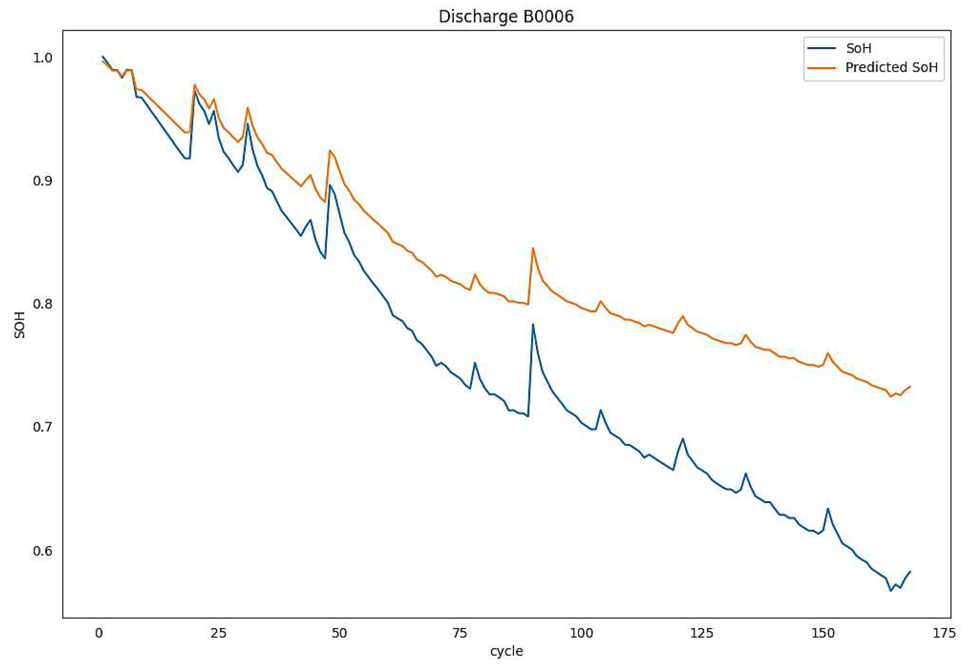
Figure 4.
Real B0006 battery SoH and its estimated SoH. The Model trained on B0005 Battery.
Another setup of SOH predictions for the different batteries at different quantization levels was executed to illustrate the accuracy of the suggested quantization on the estimated SoH. Table 6 displays relevant results. RMSE, MAE, and MAPE are used as error evaluation measures. The table shows SOH predictions from deep learning models for batteries B0006, B0007, and B0018 with different quantization bits assigned. Figure 5 shows SoH prediction without and with quantization for all bits, as b = 2, 3, 4, 5, 6, 7, and 8 bits when tested on both models, the FFNN and the LSTM.
To supplement the preceding results, a visual comparison between the quantized and real inferences was prepared. Figure 6 illustrates the comparison between the original estimated SoH and its quantized counterparts for 2 bits and 5-bit.
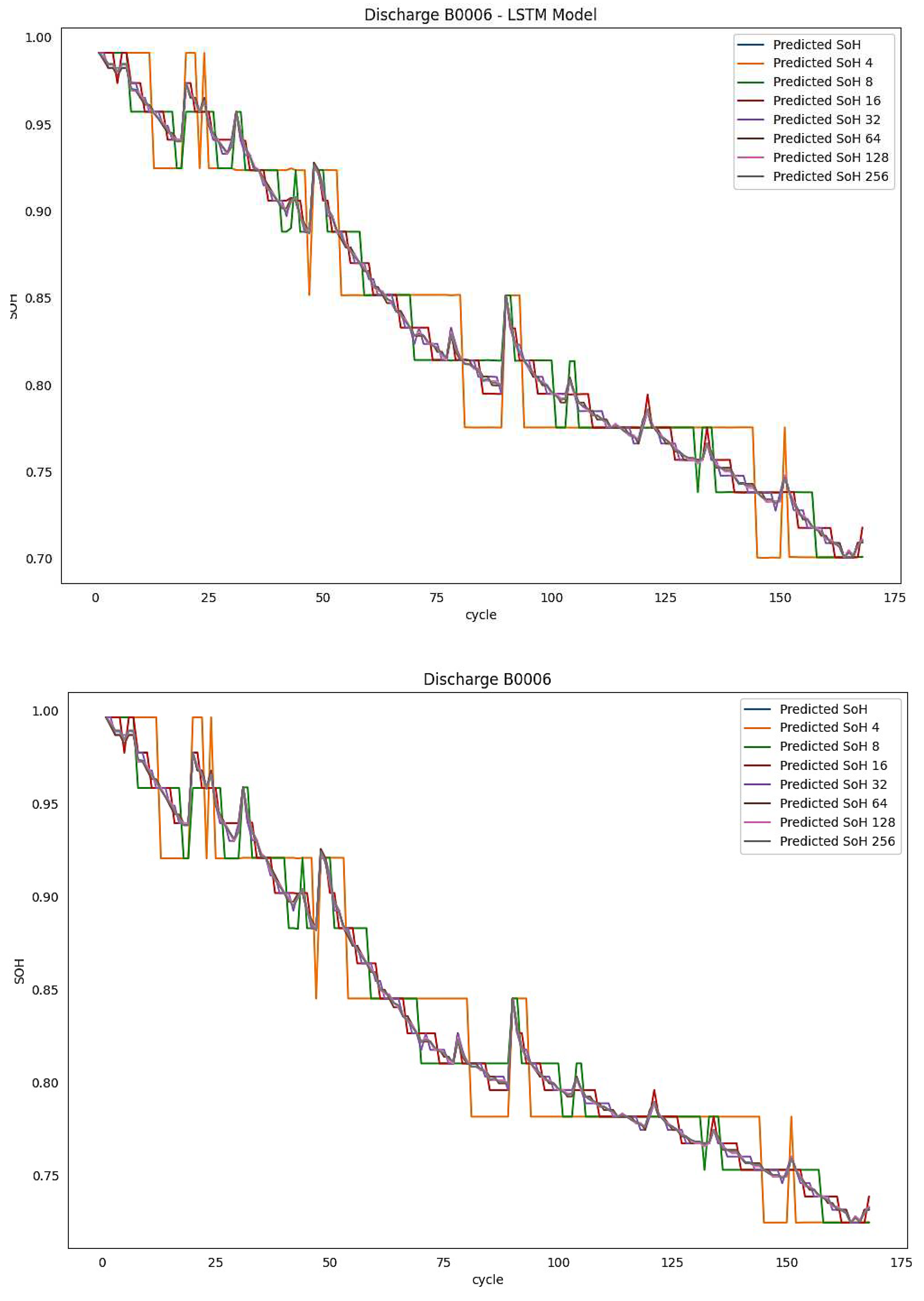
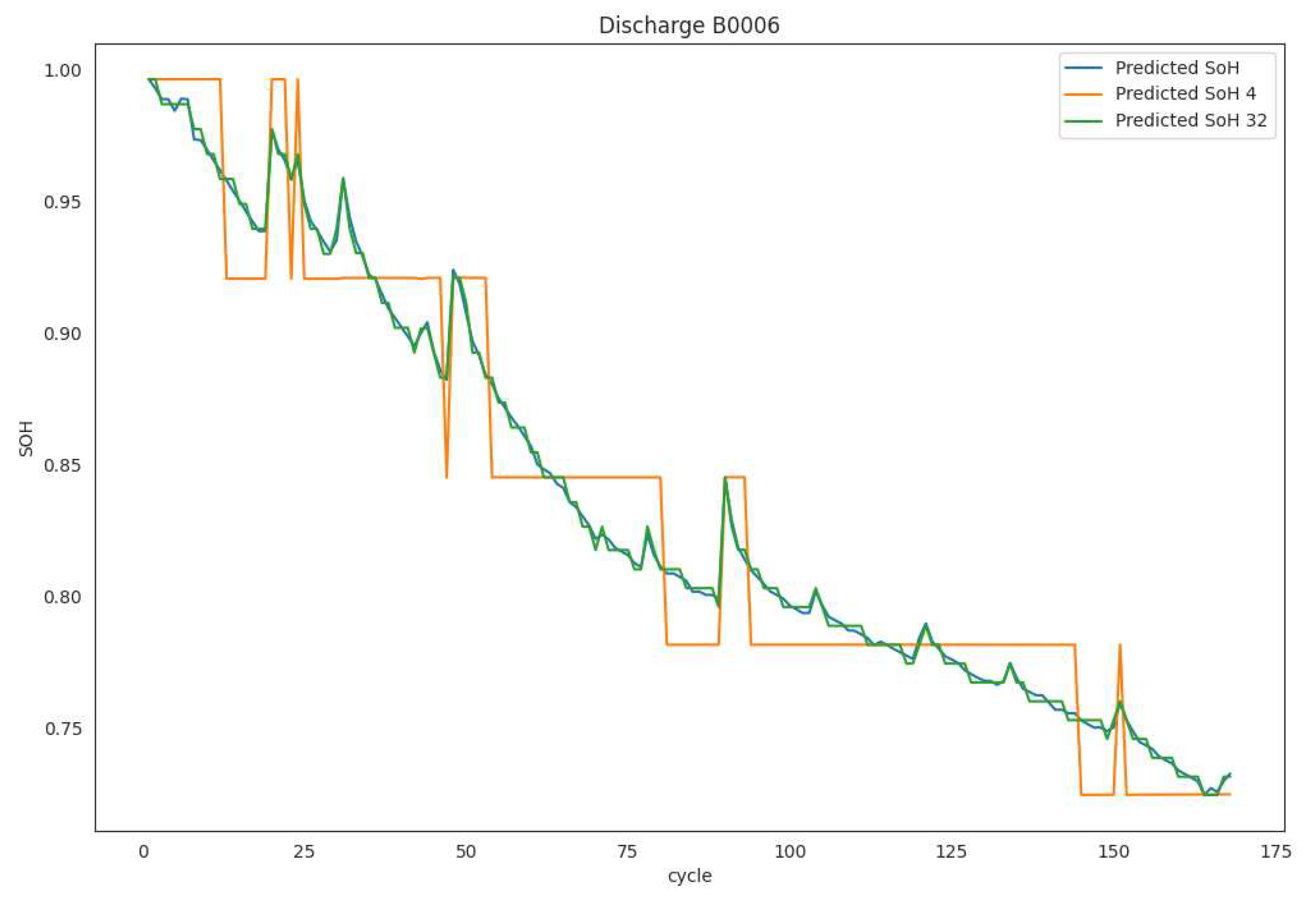
Figure 5.
SoH predictions for B0006 Battery Dataset trained on B0005 Battery dataset showing original SoH (above) and all quantized bits for FFN and LSTM models (bottom).
Figure 5.
SoH predictions for B0006 Battery Dataset trained on B0005 Battery dataset showing original SoH (above) and all quantized bits for FFN and LSTM models (bottom).
Figure 6.
SoH predictions for B0006 Battery trained on B0005 Battery dataset showing original SoH and its 2-bit and 5-bit quantized versions.
Figure 6.
SoH predictions for B0006 Battery trained on B0005 Battery dataset showing original SoH and its 2-bit and 5-bit quantized versions.
7. Discussion
Initially, the evaluation of the training models will be conducted without incorporating quantization operations. This approach aims to provide an understanding of the outcomes in their unaltered state, prior to exploring the impact of quantization. The tight correspondence between the projected state of health (SoH) and the observed SoH for battery B0006 is shown in Figure 4. This phenomenon is expected to be applicable to all other batteries, despite the lack of empirical evidence, as it has been observed.
According to the findings presented in Table 4, it is evident that the two training models exhibit significant differences in terms of elapsed training time, although having identical batch sizes and epochs. The rationale behind this observation stems from the architectural differences between LSTM and FFNN models. Specifically, the LSTM model possesses a significantly larger building structure, consisting of over 1.14 million parameters that need to be mathematically computed. In contrast, the FFNN model exhibits a much smaller parameter count, totaling only 217.
Table 5 presents the outcomes of the estimation error analysis for the Feedforward Neural Network (FFNN) training model. The model was trained on the B0005 battery and subsequently evaluated on different batteries using actual model validation, without employing quantization. Divergent error estimations are detected across the two training models across different battery types. In the B0006 battery, the root mean square error (RMSE) of the feedforward neural network (FFNN) model exhibited a superior performance compared to the long short-term memory (LSTM) model by a margin of 0.003, equivalent to a relative improvement of 4.6%. In the case of the B0007 battery, the root mean square error (RMSE) exhibited a difference favoring the LSTM model by 0.0097, which corresponds to a 50% improvement. In the case of the B0018 battery, both the FFNN and LSTM models exhibited similar performance, with a slight advantage of 0.0023 (15%) in favor of the FFNN.
The mean absolute error (MAE) metric revealed a significant disparity in performance for the B0007 battery, with an observed value of 0.0067 (37%). In contrast, the remaining batteries had similar scores in this regard. In terms of the MAPE error metric, the B0006 battery exhibited the smallest disparity with a score of 2.1%, whilst the FFNN model demonstrated the biggest disparity with a score of 42%.
Next, we will commence the examination of the impact of quantization on the state-of-health (SOH) forecasts for various batteries across different quantization levels, and analyze its influence on the accuracy of these predictions. Based on the findings presented in Table 6, it is evident that the accuracy of state-of-health (SoH) prediction utilizing quantization approaches diminishes as the number of quantization bits increases, in comparison to the original non-quantized model's SoH prediction. To provide additional support for this assertion, Figure 7 exhibits the three-error metrics in relation to the number of quantization bits for the B0006 batteries when subjected to training using FFN and LSTM models. The results demonstrate that even when employing a limited number of quantization bits, the magnitude of mistake remains quite small. Notably, the errors tend to become inconsequential after utilizing a quantization of n = 5 bits. Table 6 provides compelling evidence for the identification of distinct patterns. The findings indicate that the variations in battery types and the training models, FFN or LSTM, are inconsequential, with the primary distinguishing factor being the quantization bits.
Figure 5 presents the predictions of State of Health (SoH) without quantization, as well as with quantization for varying bit values, specifically 2, 3, 4, 5, 6, 7, and 8 bits. However, Figure 6 illustrates that the deviation from the initial prediction (before to quantization) becomes insignificant when utilizing 5 or more bits. This implies that a minimum of 5 bits is required in order to get a distinct correspondence with the prediction.
8. Summary
Battery state of health prediction using data driven models, is getting fore focused on recently. The use of machine learning and specifically deep learning has dramatically improved the SoH estimation based on recorded data. This work suggests the replacement of a Look Up Table LUT in place of the actual trained model to do an inference. The preparation of the LUT necessitates bit quantization applied on all the seven features used. It was found that accuracies were slightly affected by this adoption, when compared to the actual inferred SoH estimation without quantization. The novel finding was that b=5 bits will be mostly enough to quantize the seven features for the SoH battery prediction problem, giving a rise to a total of 35 bits. Neverthe less even with b=3 bits, the results still gave satisfactory results, and that resulted of total bits of 21 bits. This particular result made the operation of LUT very reasonable with 2 MB LUT stored in a mememory device gives almost as near results to an actual model with a full inference.
References
- Whittingham, M.S. Electrical Energy Storage and Intercalation Chemistry. Science 1976, 192, 1126–1127. [Google Scholar] [CrossRef]
- Stan, A.I.; ´Swierczy ´ nski, M.; Stroe, D.I.; Teodorescu, R.; Andreasen, S.J. Lithium Ion Battery Chemistries from Renewable Energy Storage to Automotive and Back-up Power Applications—An Overview. In Proceedings of the 2014 International Conference on Optimization of Electrical and Electronic Equipment (OPTIM), Bran, Romania, 22–24 May 2014; pp. 713–720. [Google Scholar]
- Nishi, Y. Lithium Ion Secondary Batteries; Past 10 Years and the Future. J. Power Sources 2001, 100, 101–106. [Google Scholar] [CrossRef]
- Huang, S.C.; Tseng, K.H.; Liang, J.W.; Chang, C.L.; Pecht, M.G. An Online SOC and SOH Estimation Model for Lithium-Ion Batteries. Energies 2017, 10, 512. [Google Scholar] [CrossRef]
- Goodenough, J.B.; Kim, Y. Challenges for Rechargeable Li Batteries. Chem. Mater. 2010, 22, 587–603. [Google Scholar] [CrossRef]
- Nitta, N.; Wu, F.; Lee, J.T.; Yushin, G. Li-Ion Battery Materials: Present and Future. Mater. Today 2015, 18, 252–264. [Google Scholar] [CrossRef]
- Dai, H.; Jiang, B.; Hu, X.; Lin, X.; Wei, X.; Pecht, M. Advanced Battery Management Strategies for a Sustainable Energy Future: Multilayer Design Concepts and Research Trends. Renew. Sustain. Energ. Rev. 2021, 138, 110480. [Google Scholar] [CrossRef]
- Lawder, M.T.; Suthar, B.; Northrop, P.W.; De, S.; Hoff, C.M.; Leitermann, O.; Crow, M.L.; Santhanagopalan, S.; Subramanian, V.R. Battery Energy Storage System (BESS) and Battery Management System (BMS) for Grid-Scale Applications. Proc. IEEE 2014, 102, 1014–1030. [Google Scholar] [CrossRef]
- Lai, X.; Gao, W. A comparative study of global optimization methods for parameter identification of different equivalent circuit models for Li-ion batteries. Electrochim. Acta 2019, 295, 1057–1066. [Google Scholar] [CrossRef]
- Wang, Y.; Gao, G.; Li, X.; Chen, Z. A fractional-order model-based state estimation approach for lithium-ion battery and ultra-capacitor hybrid power source system considering load trajectory. J. Power Sources 2020, 449, 227543. [Google Scholar] [CrossRef]
- Cheng, G.; Wang, X.; He, Y. Remaining useful life and state of health prediction for lithium batteries based on empirical mode decomposition and a long and short memory neural network. Energy 2021, 232, 121022. [Google Scholar] [CrossRef]
- Rechkemmer, S.; Zang, X. Empirical Li-ion aging model derived from single particle model. J. Energy Storage 2019, 21, 773–786. [Google Scholar] [CrossRef]
- Li, K.; Wang, Y.; Chen, Z. A comparative study of battery state-of-health estimation based on empirical mode decomposition and neural network. J. Energy Storage 2022, 54, 105333. [Google Scholar] [CrossRef]
- Geng, Z.; Wang, S.; Lacey, M.J.; Brandell, D.; Thiringer, T. Bridging physics-based and equivalent circuit models for lithium-ion batteries. Electrochim. Acta 2021, 372, 137829. [Google Scholar] [CrossRef]
- Xu, N.; Xie, Y.; Liu, Q.; Yue, F.; Zhao, D. A Data-Driven Approach to State of Health Estimation and Prediction for a Lithium-Ion Battery Pack of Electric Buses Based on Real-World Data. Sensors 2022, 22, 5762. [Google Scholar] [CrossRef] [PubMed]
- Alipour, M.; Tavallaey, S. Improved Battery Cycle Life Prediction Using a Hybrid Data-Driven Model Incorporating Linear Support Vector Regression and Gaussian. ChemPhysChem 2022, 23, e202100829. [Google Scholar] [CrossRef]
- Li, X.; Wang, Z. Prognostic health condition for lithium battery using the partial incremental capacity and Gaussian process regression. J. Power Sources 2019, 421, 56–67. [Google Scholar] [CrossRef]
- Li, Y.; Abdel-Monem, M. A quick on-line state of health estimation method for Li-ion battery with incremental capacity curves processed by Gaussian filter. J. Power Sources 2018, 373, 40–53. [Google Scholar] [CrossRef]
- Onori, S.; Spagnol, P.; Marano, V.; Guezennec, Y.; Rizzoni, G. A New Life Estimation Method for Lithium-Ion Batteries in Plug-in Hybrid Electric Vehicles Applications. Int. J. Power Electron. 2012, 4, 302–319. [Google Scholar] [CrossRef]
- Plett, G.L. Extended Kalman Filtering for Battery Management Systems of LiPB-Based HEV Battery Packs: Part State and Parameter Estimation. J. Power Sources 2004, 134, 277–292. [Google Scholar] [CrossRef]
- Goebel, K.; Saha, B.; Saxena, A.; Celaya, J.R.; Christophersen, J.P. Prognostics in Battery Health Management. IEEE Instrum. Meas. Mag 2008, 11, 33–40. [Google Scholar] [CrossRef]
- Wang, D.; Yang, F.; Zhao, Y.; Tsui, K.L. Battery Remaining Useful Life Prediction at Different Discharge Rates. Microelectron. Reliab. 2017, 78, 212–219. [Google Scholar] [CrossRef]
- Li, J.; Landers, R.G.; Park, J. A Comprehensive Single-Particle-Degradation Model for Battery State-of-Health Prediction. J. Power Sources 2020, 456, 227950. [Google Scholar] [CrossRef]
- Hu, X.; Jiang, J.; Cao, D.; Egardt, B. Battery Health Prognosis for Electric Vehicles Using Sample Entropy and Sparse Bayesian Predictive Modeling. IEEE Trans. Ind. Electron. 2015, 63, 2645–2656. [Google Scholar] [CrossRef]
- Piao, C.; Li, Z.; Lu, S.; Jin, Z.; Cho, C. Analysis of Real-Time Estimation Method Based on Hidden Markov Models for Battery System States of Health. J. Power Electron. 2016, 16, 217–226. [Google Scholar] [CrossRef]
- Liu, D.; Pang, J.; Zhou, J.; Peng, Y.; Pecht, M. Prognostics for State of Health Estimation of Lithium-Ion Batteries Based on Combination Gaussian Process Functional Regression. Microelectron. Reliab. 2013, 53, 832–839. [Google Scholar] [CrossRef]
- Khumprom, P.; Yodo, N. A Data-Driven Predictive Prognostic Model for Lithium-Ion Batteries Based on a Deep Learning Algorithm. Energies 2019, 12, 660. [Google Scholar] [CrossRef]
- Xia, Z.; Qahouq, J.A.A. Adaptive and Fast State of Health Estimation Method for Lithium-Ion Batteries Using Online Complex Impedance and Artificial Neural Network. In Proceedings of the 2019 IEEE Applied Power Electronics Conference and Exposition (APEC), Anaheim, CA, USA, 17–21 March 2019; pp. 3361–3365. [Google Scholar]
- Eddahech, A.; Briat, O.; Bertrand, N.; Delétage, J.Y.; Vinassa, J.M. Behavior and State-of-Health Monitoring of Li-Ion Batteries Using Impedance Spectroscopy and Recurrent Neural Networks. Int. J. Electr. Power Energy Syst. 2012, 42, 487–494. [Google Scholar] [CrossRef]
- Shen, S.; Sadoughi, M.; Chen, X.; Hong, M.; Hu, C. A Deep Learning Method for Online Capacity Estimation of Lithium-Ion Batteries. J. Energy Storage 2019, 25, 100817. [Google Scholar] [CrossRef]
- Saha, B.; Goebel, K. Battery Data Set, NASA Ames Prognostics Data Repository; NASA Ames Research Center: Moffett Field, CA, USA, 2007; Available online: https://ti.arc.nasa.gov/tech/dash/groups/pcoe/prognostic-data-repository/ (accessed on 25 September 2020).
- Ren, L.; Zhao, L.; Hong, S.; Zhao, S.; Wang, H.; Zhang, L. Remaining Useful Life Prediction for Lithium-Ion Battery: A Deep Learning Approach. IEEE Access 2018, 6, 50587–50598. [Google Scholar] [CrossRef]
- Khumprom, P.; Yodo, N. A Data-Driven Predictive Prognostic Model for Lithium-Ion Batteries Based on a Deep Learning Algorithm. Energies 2019, 12, 660. [Google Scholar] [CrossRef]
- Choi, Y.; Ryu, S.; Park, K.; Kim, H. Machine Learning-Based Lithium-Ion Battery Capacity Estimation Exploiting Multi-Channel Charging Profiles. IEEE Access 2019, 7, 75143–75152. [Google Scholar] [CrossRef]
- Ruihao Gong, Xianglong Liu, Shenghu Jiang, Tianxiang Li,Peng Hu, Jiazhen Lin, Fengwei Yu, and Junjie Yan. Differentiablesoft quantization: Bridging full-precision and low-bitneural networks. In ICCV, pages 4852–4861, 2019. 1, 2, 5,6.
- Jungwook Choi, Zhuo Wang, Swagath Venkataramani,Pierce I-Jen Chuang, Vijayalakshmi Srinivasan, and KailashGopalakrishnan. Pact: Parameterized clipping activation forquantized neural networks. arXiv, 2018. 1, 2, 5, 6.
- Steven K Esser, Jeffrey L McKinstry, Deepika Bablani,Rathinakumar Appuswamy, and Dharmendra S Modha.Learned step size quantization. In ICLR, 2019. 1, 2, 4, 5,6.
- Zhaohui Yang, Yunhe Wang, Kai Han, Chunjing Xu, ChaoXu, Dacheng Tao, and Chang Xu. Searching for low-bitweights in quantized neural networks. In NeurIPS, 2020.1, 2, 5.
- Matthieu Courbariaux, Yoshua Bengio, and Jean-PierreDavid. Binaryconnect: Training deep neural networks withbinary weights during propagations. In NeurIPS, 2017. 2.
- Chenzhuo Zhu, Song Han, Huizi Mao, and William J Dally.Trained ternary quantization. In ICLR, 2017. 2.
- Mohammad Rastegari, Vicente Ordonez, Joseph Redmon,and Ali Farhadi. Xnor-net: Imagenet classification using binaryconvolutional neural networks. In ECCV, pages 525–542, 2016. 2.
- Karen Ullrich, Edward Meeds, and Max Welling. Softweight-sharing for neural network compression. In ICLR,2017. 2.
- Yuhui Xu, YongzhuangWang, Aojun Zhou,Weiyao Lin, andHongkai Xiong. Deep neural network compression with singleand multiple level quantization. In AAAI, volume 32,2018. 2.
- Aojun Zhou, Anbang Yao, Yiwen Guo, Lin Xu, and YurongChen. Incremental network quantization: Towards losslesscnns with low-precision weights. In ICLR, 2017. 2.
- Daisuke Miyashita, Edward H Lee, and Boris Murmann.Convolutional neural networks using logarithmic data representation.ar Xiv, 2016. 2.
- Davis Blalock, Jose Javier Gonzalez Ortiz, Jonathan Frankle, and John Guttag. 2020. What is the state of neural network pruning? Proceedings of machine learning and systems 2 (2020), 129–146.
- Jianping Gou, Baosheng Yu, Stephen J Maybank, and Dacheng Tao.2021. Knowledge distillation: A survey. International Journal of Computer Vision 129 (2021), 1789–1819.
- Google. 2019. TensorFlow: An end-to-end open source machine learningplatform. https://www.tensorflow.org/.
- MACE. 2020. https://github.com/XiaoMi/mace.
- Microsoft. 2019. ONNX Runtime. https://github.com/microsoft/.
- Manni Wang, Shaohua Ding, Ting Cao, Yunxin Liu, and Fengyuan Xu. 2021. Asymo: scalable and efficient deep-learning inference on asymmetric mobile CPUs. In Proceedings of the 27th Annual International Conference on Mobile Computing and Networking. 215–228.
- Tianqi Chen, Thierry Moreau, Ziheng Jiang, Lianmin Zheng, Eddie Yan, Haichen Shen, Meghan Cowan, Leyuan Wang, Yuwei Hu, LuisCeze, et al. 2018. TVM: An automated end-to-end optimizing compiler for deep learning. In 13th USENIX Symposium on Operating Systems Design and Implementation (OSDI 18). 578–594.
- Rendong Liang, Ting Cao, Jicheng Wen, Manni Wang, Yang Wang, Jianhua Zou, and Yunxin Liu. 2022. Romou: Rapidly generate high performance tensor kernels for mobile gpus. In Proceedings of the 28thAnnual International Conference on Mobile Computing And Networking.487–500.
- Yang Jiao, Liang Han, and Xin Long. 2020. Hanguang 800 NPU - The Ultimate AI Inference Solution for Data Centers. In IEEE Hot Chips 32Symposium, HCS 2020, Palo Alto, CA, USA, August 16-18, 2020. IEEE,1–29. [CrossRef]
- Norman P. Jouppi, Doe Hyun Yoon, Matthew Ashcraft, Mark Gottscho, Thomas B. Jablin, George Kurian, James Laudon, Sheng Li, Peter Ma, Xiaoyu Ma, Thomas Norrie, Nishant Patil, Sushma Prasad, Cliff Young, Zongwei Zhou, and David Patterson. 2021. Ten Lessons from Three Generations Shaped Google’s TPUv4i (ISCA ’21). IEEE Press, 1–14. [CrossRef]
- Ofri Wechsler, Michael Behar, and Bharat Daga. 2019. Spring Hill(NNP-I 1000) Intel’s Data Center Inference Chip. In 2019 IEEE Hot Chips 31 Symposium (HCS). 1–12. [CrossRef]
Figure 1.
Degradation of lithium-ion batteries as a function of cycle count.
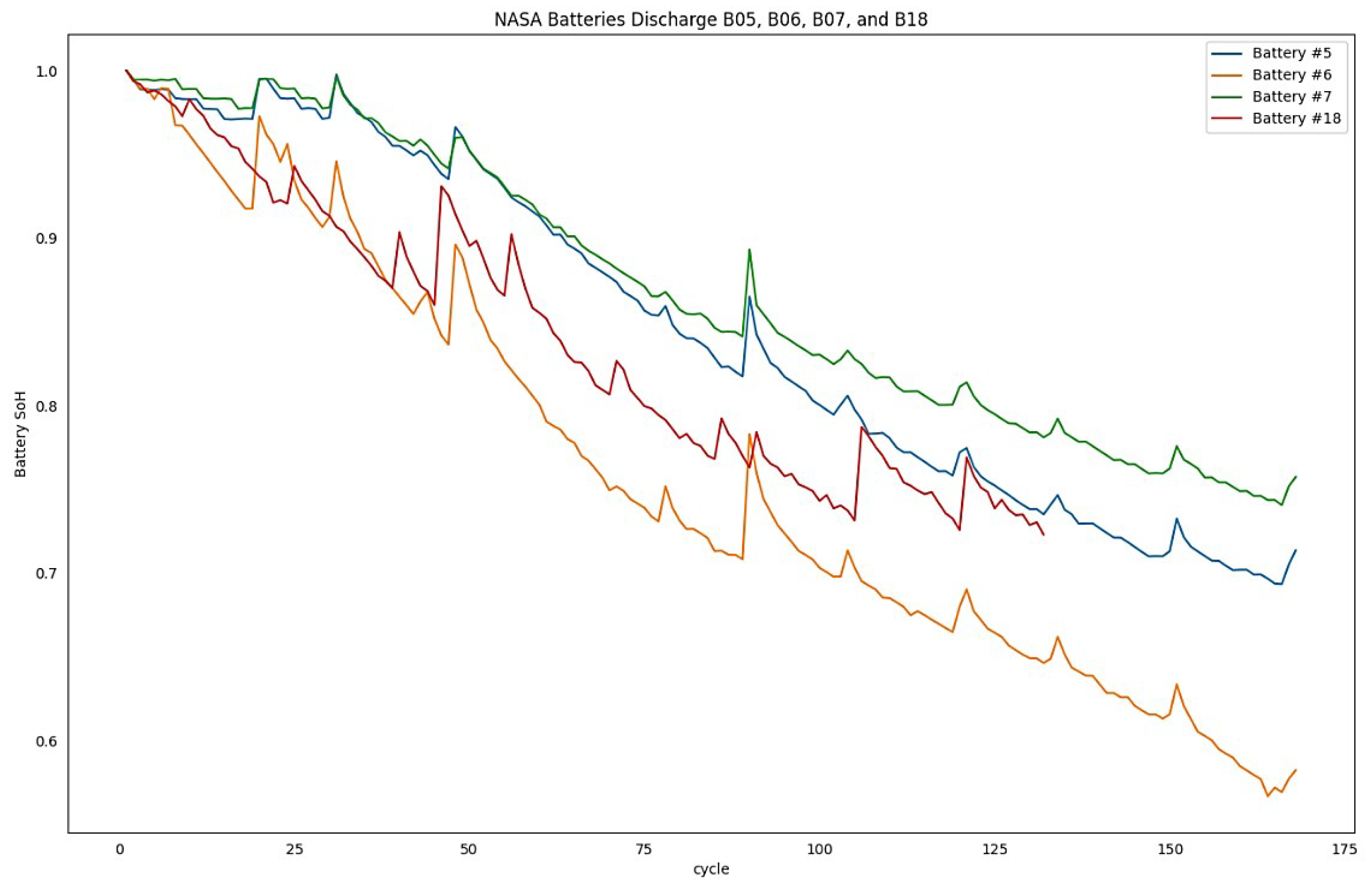
Figure 2.
(Upper) Deep Feed Forwards Neural Network (FFNN) and (Lower) Long Short-Term Memory (LSTM).
Figure 2.
(Upper) Deep Feed Forwards Neural Network (FFNN) and (Lower) Long Short-Term Memory (LSTM).
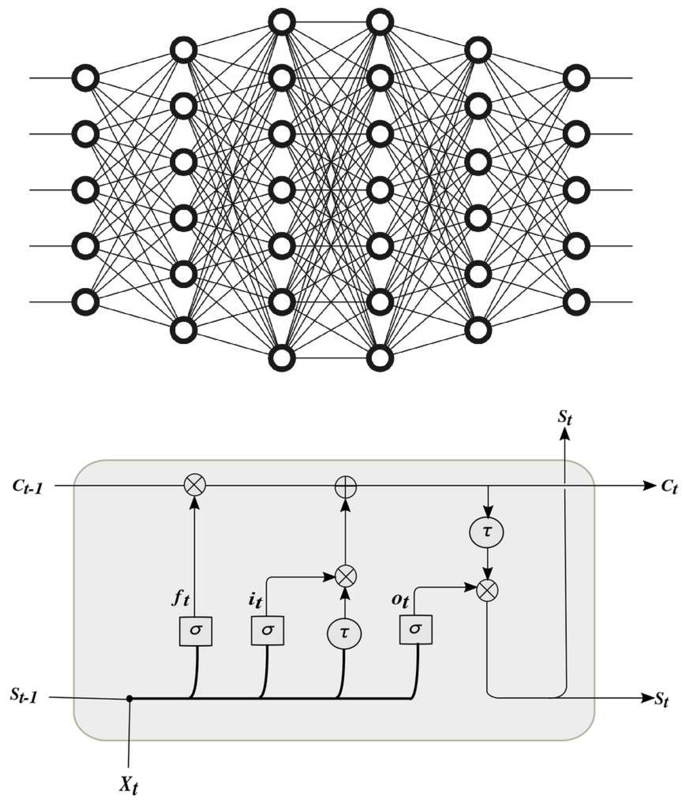
Figure 3.
The new algorithm flowchart and features-bit distribution.
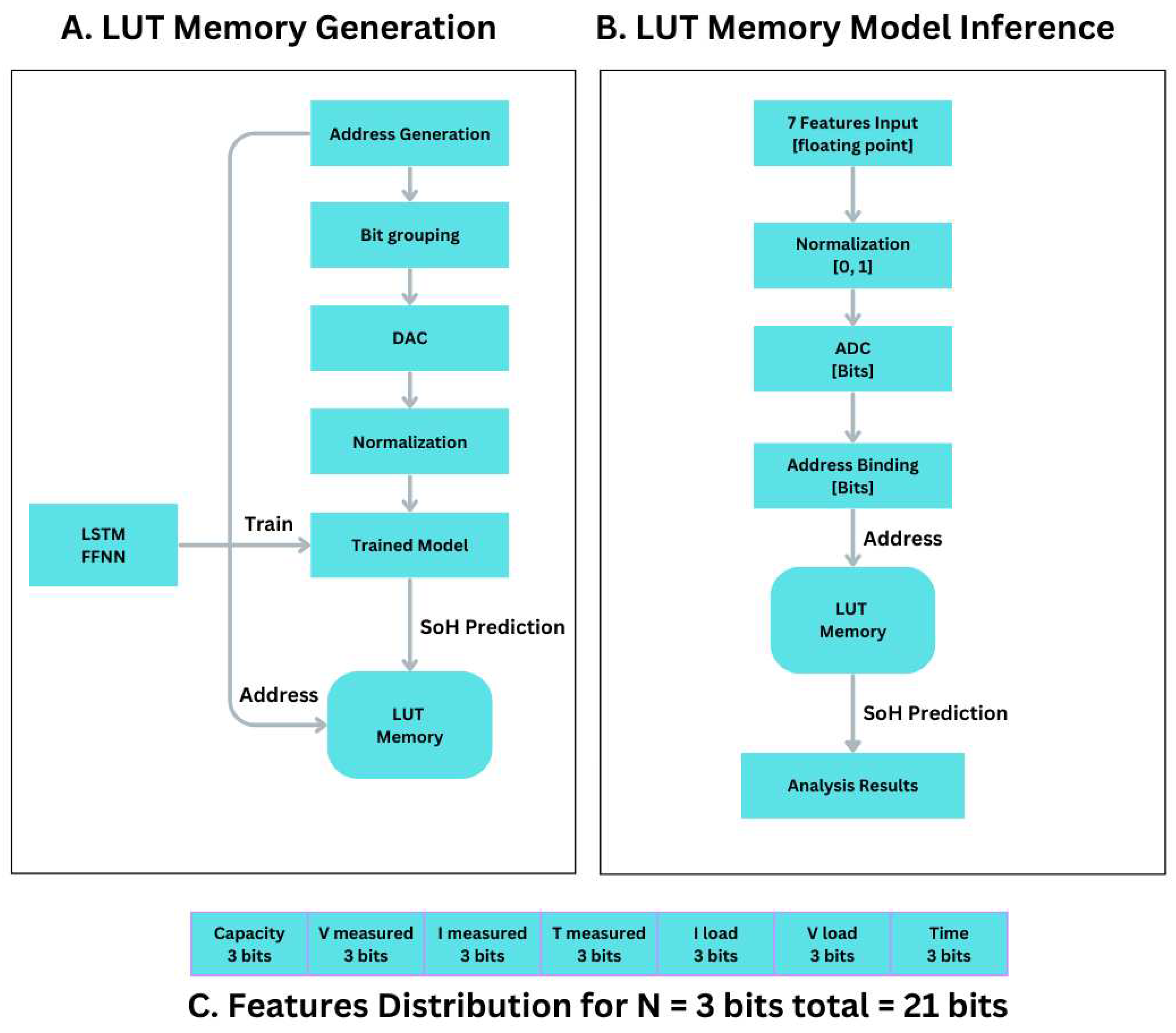
Figure 7.
Effect of Quantization on SoH prediction error for B006 battery trained with FFN and LSTM models respectively.
Figure 7.
Effect of Quantization on SoH prediction error for B006 battery trained with FFN and LSTM models respectively.
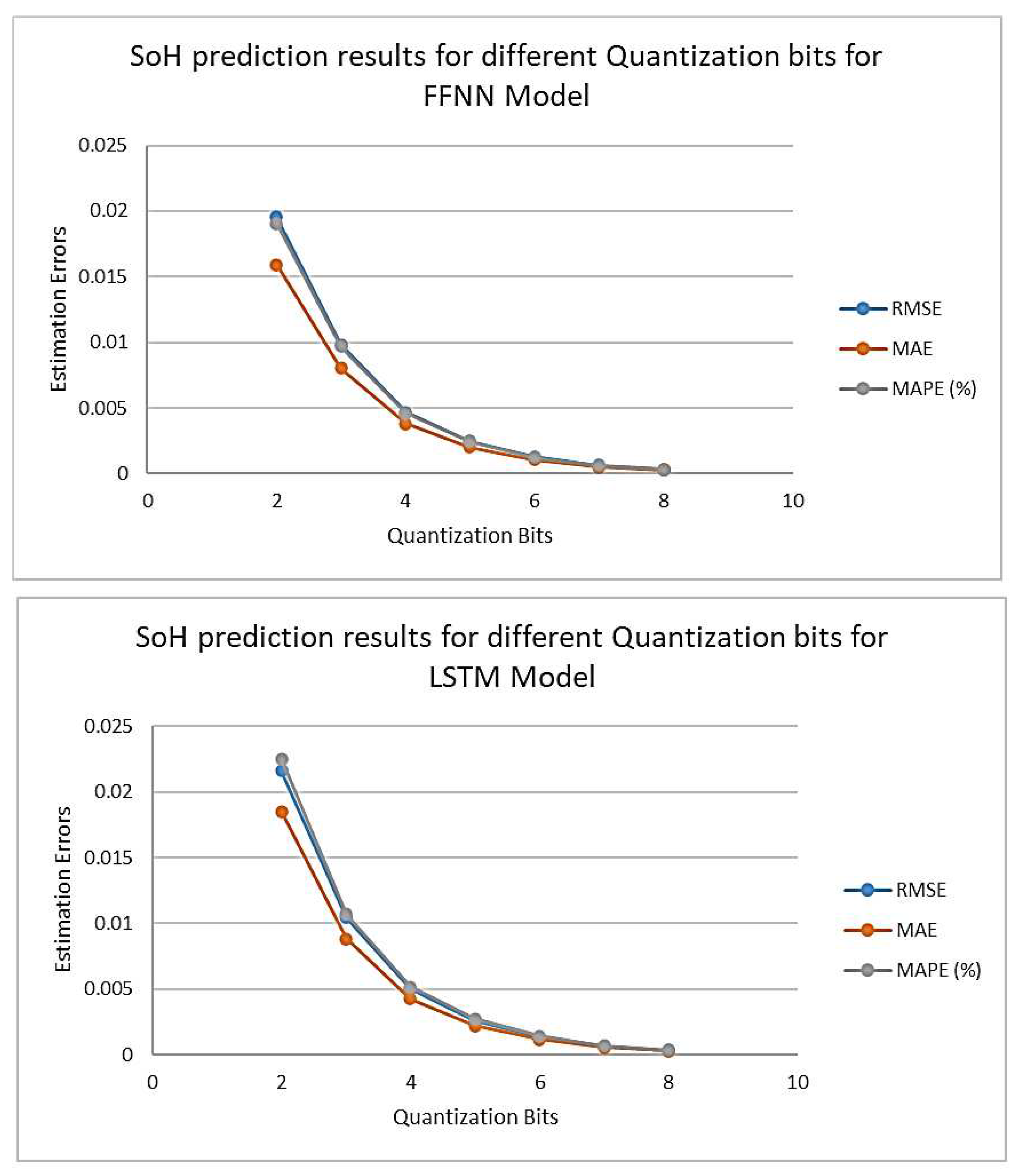

Table 1.
Boundaries of the measured features for B0005 Battery.
| Capacity | Vm | Im | Tm | ILoad | VLoad | Time (s) | |
|---|---|---|---|---|---|---|---|
| Min | 1.28745 | 2.44567 | -2.02909 | 23.2148 | -1.9984 | 0.0 | 0 |
| Max | 1.85648 | 4.22293 | 0.00749 | 41.4502 | 1.9984 | 4.238 | 3690234 |
Table 2.
Training Model Specification.
|
Model 1 FFNN |
Layers | Output Shape | Parameters No. |
| Dense | (node, 8) | 217 | |
| Dense | (node, 8) | ||
| Dense | (node, 8) | ||
| Dense | (node, 8) | ||
| Dense | (node, 1) | ||
| Layers | Output Shape | Parameters No. | |
|
Model 2 LSTM |
LSTM 1 | (N, 7, 200) | 1.124 M |
| Dropout 1 | (N, 7, 200) | ||
| LSTM 2 | (7, 200) | ||
| Dropout 2 | (N, 7, 200) | ||
| LSTM 3 | (N, 7, 200) | ||
| Dropout 3 | (N, 7, 200) | ||
| LSTM 4 | (N, 200) | ||
| Dropout 4 | (N, 200) | ||
| Dense | (N, 1) |
Table 3.
Quantization bits distribution per feature and corresponding SQNR level and total memory size needed.
Table 3.
Quantization bits distribution per feature and corresponding SQNR level and total memory size needed.
| Bits / Feature | Values given | Bits Total (Address) |
SQNR dB |
Memory Size |
|---|---|---|---|---|
| 2 | 4 | 14 | 12.04 | 16K |
| 3 | 8 | 21 | 18.06 | 2M |
| 4 | 16 | 28 | 24.08 | 256M |
| 5 | 32 | 35 | 30.10 | 32G |
| 6 | 64 | 42 | 36.12 | 4T |
| 7 | 128 | 49 | 42.14 | ---- |
| 8 | 256 | 56 | 48.16 | ---- |
Table 4.
Training Parameters for B0005 Battery Dataset.
| Model | Batch size | Epochs | Time(s) | Loss |
|---|---|---|---|---|
| FFNN | 25 | 50 | 200 | 0.0243 |
| LSTM | 25 | 50 | 7453 | 3.1478E-05 |
Table 5.
Estimation errors results for FFNN training model when trained on B0005 Battery and tested on the others using actual model validation (testing) without quantization.
Table 5.
Estimation errors results for FFNN training model when trained on B0005 Battery and tested on the others using actual model validation (testing) without quantization.
| Battery | Model | RMSE | MAE | MAPE |
|---|---|---|---|---|
| B0006 | FFNN | 0.080010 | 0.068220 | 0.100970 |
| LSTM | 0.076270 | 0.067620 | 0.098770 | |
| B0007 | FFNN | 0.019510 | 0.018019 | 0.021460 |
| LSTM | 0.029282 | 0.024710 | 0.030434 | |
| B0018 | FFNN | 0.015680 | 0.013610 | 0.016890 |
| LSTM | 0.018021 | 0.016371 | 0.020547 |
Table 6.
Prediction results after comparing between SoH of Non-Quantized and the Quantized versions based on different models for batteries B0006, B0007, and B0018.
Table 6.
Prediction results after comparing between SoH of Non-Quantized and the Quantized versions based on different models for batteries B0006, B0007, and B0018.
| Battery | Model | Quantization Bits | RMSE | MAE | MAPE (%) |
|---|---|---|---|---|---|
| B0006 | FFNN | 2 | 0.0195370 | 0.0159236 | 0.0190499 |
| 3 | 0.0098006 | 0.0080317 | 0.0096645 | ||
| 4 | 0.0046815 | 0.0037988 | 0.0045664 | ||
| 5 | 0.0024301 | 0.0020093 | 0.0024294 | ||
| 6 | 0.0012535 | 0.0010379 | 0.0012461 | ||
| 7 | 0.0006150 | 0.0005068 | 0.0006144 | ||
| 8 | 0.0003125 | 0.0002565 | 0.0003088 | ||
| LSTM | 2 | 0.0216045 | 0.0185078 | 0.0225291 | |
| 3 | 0.0104658 | 0.0088477 | 0.0107360 | ||
| 4 | 0.0050010 | 0.0042487 | 0.0051737 | ||
| 5 | 0.0025885 | 0.0022293 | 0.0027206 | ||
| 6 | 0.0013394 | 0.0011620 | 0.0014114 | ||
| 7 | 0.0006609 | 0.0005692 | 0.0006974 | ||
| 8 | 0.0003309 | 0.0002835 | 0.0003446 | ||
| B0007 | FFNN | 2 | 0.0187614 | 0.0162685 | 0.0191451 |
| 3 | 0.0101181 | 0.0088282 | 0.0103004 | ||
| 4 | 0.0050026 | 0.0043651 | 0.0051114 | ||
| 5 | 0.0024498 | 0.0021127 | 0.0024730 | ||
| 6 | 0.0012030 | 0.0010481 | 0.0012269 | ||
| 7 | 0.0006394 | 0.0005566 | 0.0006533 | ||
| 8 | 0.0003060 | 0.0002578 | 0.0003013 | ||
| LSTM | 2 | 0.0209633 | 0.0181984 | 0.0219105 | |
| 3 | 0.0113147 | 0.0099692 | 0.0119157 | ||
| 4 | 0.0056382 | 0.0049296 | 0.0059140 | ||
| 5 | 0.0027386 | 0.0023843 | 0.0028542 | ||
| 6 | 0.0013495 | 0.0011826 | 0.0014153 | ||
| 7 | 0.0007212 | 0.0006320 | 0.0007581 | ||
| 8 | 0.0003432 | 0.0002912 | 0.0003475 | ||
| B00018 | FFNN | 2 | 0.0205289 | 0.0159912 | 0.0189426 |
| 3 | 0.0096451 | 0.0077552 | 0.0092191 | ||
| 4 | 0.0050730 | 0.0040254 | 0.0047780 | ||
| 5 | 0.0022966 | 0.0017585 | 0.0020886 | ||
| 6 | 0.0011492 | 0.0008754 | 0.0010336 | ||
| 7 | 0.0006432 | 0.0005005 | 0.0005950 | ||
| 8 | 0.0002954 | 0.0002268 | 0.0002719 | ||
| LSTM | 2 | 0.0218554 | 0.0189299 | 0.0233109 | |
| 3 | 0.0109069 | 0.0094792 | 0.0116619 | ||
| 4 | 0.0057440 | 0.0049472 | 0.0060704 | ||
| 5 | 0.0026591 | 0.0022228 | 0.0027317 | ||
| 6 | 0.0013255 | 0.0011411 | 0.0014012 | ||
| 7 | 0.0007168 | 0.0006208 | 0.0007612 | ||
| 8 | 0.0003431 | 0.0002941 | 0.0003649 |
Disclaimer/Publisher’s Note: The statements, opinions and data contained in all publications are solely those of the individual author(s) and contributor(s) and not of MDPI and/or the editor(s). MDPI and/or the editor(s) disclaim responsibility for any injury to people or property resulting from any ideas, methods, instructions or products referred to in the content. |
© 2023 by the authors. Licensee MDPI, Basel, Switzerland. This article is an open access article distributed under the terms and conditions of the Creative Commons Attribution (CC BY) license (http://creativecommons.org/licenses/by/4.0/).
Copyright: This open access article is published under a Creative Commons CC BY 4.0 license, which permit the free download, distribution, and reuse, provided that the author and preprint are cited in any reuse.


