Submitted:
17 November 2023
Posted:
20 November 2023
You are already at the latest version
Abstract
Since sensor-based perception systems are used in autonomous vehicle applications, validating such systems is imperative to guarantee the robustness of the systems before they are being put to use. In this study, a comprehensive corruption-related simulation-based robustness verification and enhancement process for sensor-based perception systems is proposed. Firstly, we present a methodology and scenario-based corruption generation tools for creating diverse simulated test scenarios that can analogously represent real-world traffic environments, especially considering corruption types related to safety concern. Then, an effective corruption similarity filtering algorithm is proposed to remove corruption types with high similarity and identify the representative corruption types to represent all considered corruption types. As a result, we can generate efficient corruption-related robustness test scenarios with less testing time and good scenario coverage. Subsequently, we perform the vulnerability analysis of object detection models to identify model weaknesses and construct an effective training dataset for model vulnerability enhancement. This enhances the tolerance of object detection models to weather and noise-related corruptions, ultimately improving the robustness of the perception system. We employ case studies to demonstrate the feasibility and effectiveness of the proposed robustness verification and enhancement procedures. Additionally, we explore the impact of different "similarity overlap threshold" parameter settings on scenario coverage, effectiveness, scenario complexity (size of training and testing datasets), and time costs.
Keywords:
autonomous driving
; corruption factors
; perception system
; robustness verification
; scenario-based testing
1. Introduction
In recent years, as major automakers have actively pursued the development of autonomous vehicles, the requirements of design and testing validation for self-driving cars have become increasingly stringent. These vehicles must demonstrate their reliability and safety to meet the safety standards for autonomous driving. Autonomous driving systems primarily consist of four processing modules: sensor-based perception, localization, trajectory planning and control. These modules are interdependent, and the performance of the sensor-based perception system, in particular, is crucial. Insufficient robustness in this system can lead to severe traffic accidents and pose significant risks. The sensor-based perception system comprises the primary sensors, including the camera, LiDAR, and radar. These various sensors are capable of detecting environmental cues, yet each possesses its own strengths and weaknesses. The perception functionality could be susceptible to corruption or misjudgment under varying road situations, weather conditions, and traffic environments. Therefore, how to ensure that the autonomous perception system can operate safely and reliably in various driving scenarios is of utmost importance, as it will influence the reliability and safety performance of the self-driving systems [1]. The test coverage affects the testing quality of the autonomous driving systems. Increasing the coverage of rare driving situations and corner cases is thus crucial. To collect data from all possible scenarios through real-world testing would require a minimum of 275 million miles of testing mileage [2], incurring substantial costs and time, making it a challenging and economically impractical endeavor.
The methodology of testing and verification of autonomous driving systems primarily consist of simulation approach and real-world testing. Currently, we observe that many major automakers are conducting real-world road tests with autonomous vehicles. However, most of these tests are conducted in common and typical scenarios. To test for safety-critical or rare, low-probability adverse driving scenarios and corner cases, one must contend with certain risks and substantial costs and time. Even when there is an opportunity to test rare combinations of factors such as weather, lighting, traffic conditions, and sensor noise corruption that lead to failures in autonomous perception systems [3–5], replicating the same real-world testing conditions remains challenging and infeasible.
On the other hand, vehicle simulation approach allows for the rapid creation of various test scenarios, including adjustments to different weather conditions within the same test scenario. The advantages of simulation are easy to build the desired scenarios and perform the scenario-based testing with lower cost and safe manner. Presently, there are various vehicle simulation tools available, such as Vires Virtual Test Drive (VTD) [6] , IPG Automotive CarMaker[7] , CARLA [8], etc. However, the soundness of test results depends on the accuracy of simulating sensors, vehicles, and environments. For instance, simulating rainfall involves adjusting rainfall model parameters like intensity, and the challenge is how to match real-world rainfall conditions, such as an hourly rainfall rate, for example 20 mm/h in the simulation environment. Additionally, the modeling accuracy of simulating cameras installed behind the windshield of autonomous vehicles is limited by factors like raindrops affecting the camera's view, which cannot be fully replicated at present.
In the context of autonomous driving perception systems, object detection is of paramount importance. Any failure or anomaly in object detection can significantly affect the system's prediction and decision-making processes, potentially leading to hazardous situations. Therefore, extensive testing and verification must be conducted under various condition combinations. According to ISO 26262 standards, autonomous driving systems are allowed a maximum of one failure per kilometers driven, making it impractical to conduct real-world testing and verification [9].
Currently, there are several real traffic image datasets available, such as nuScenes [10], BDD100K [11], Cityscapes [12], KITTI [13], etc., which assist in training and verifying object detection models. However, these datasets still cannot cover all possible environmental influences. Some image datasets are recorded only under favorable weather conditions, and moreover the scenario parameters cannot be quantified to understand the severity of the corruption types including weather-related and noise-related factors and their impact on the object detection capability.
Adverse weather conditions can lead to a decrease in object detection accuracy. In addition, when camera noise appears in the image, even a single-pixel corruption has the potential to cause errors or failures in the object detection [14]. This, in turn, can result in erroneous judgments during autonomous vehicle operation. Presently, there is no comprehensive and quantifiable benchmark test dataset for adverse weather and image noise corruption conditions, which could provide adequate test coverage for the verification process of the autonomous driving systems.
While there has been related research using vehicle simulation environments to test and verify advanced driver-assistance systems by adjusting various weather, lighting, and camera conditions, it still lacks for simulating the scenarios where raindrops interfere with the image lens mounted behind the windshield and the severity effect of image lens corruption on image quality. In real-world situations, this can affect object detection accuracy. Hence, leveraging the advantages of simulation and establishing effective benchmark test datasets for testing and verification, and improving the reliability and robustness of autonomous vehicle perception systems is a topic worthy of exploration.
This study primarily explores how to integrate raindrops falling on the windshield and various types of weather-related and noise-related corruptions into scenarios in the simulation environment. By adjusting weather-related and noise-related parameters, it aims to establish an effective benchmark test dataset to aid in testing and verifying the reliability and robustness of object detection models. Furthermore, through this benchmark test dataset, the study intends analyzing the vulnerabilities of object detection models. This analysis will help designers identify areas of improvement and propose enhanced training datasets for transfer learning, thereby enhancing model robustness and reliability.
The primary challenge here lies in the complexity of scenarios involving single corruption factors and combinations of multiple corruption factors, resulting in a considerable volume of test data and time cost for verification. To facilitate rapid testing and verification in the early stage of system development while ensuring the quality of the test dataset, this work introduces a corruption similarity analysis algorithm. This algorithm explores the similarity of different corruptions and relies on the setup of overlapping threshold value to reduce corruption types with higher similarity. The choice of overlapping threshold value affects the number of retained corruption types, the size of training and test datasets, training and verification time, and test coverage. By analyzing these factors, appropriate "corruption overlapping threshold" can be set to obtain an optimal benchmark test dataset that meets the requirements of time cost and test scenario coverage, considering both cost-effectiveness and testing quality.
The remaining paper is organized as follows. In Section 2, the related works are summarized. An effective methodology of corruption-related simulation-based testing scenario benchmark generation for robustness verification and enhancement is proposed in Section 3. Then, we analyze and discuss the experimental results in Section 4. The conclusions appear in Section 5.
2. Related Works
The actual road testing and validation of autonomous vehicles may require covering several million kilometers to gather performance statistics, primarily relevant to mechanical configurations and algorithm parameters. However, this approach is less effective during the development process, such as the V model development workflow [15]. Nevertheless, the testing and validation of autonomous driving functions necessitate various complex traffic scenarios, including uncertainties associated with other vehicles or motorcycles. Adjusting parameter variations for different scenarios is more easily achieved through simulation and emulation, facilitating broader coverage of traffic scenarios, and enabling repeatable test runs with traceable experimental results. Relying solely on the total mileage driven for the validation of autonomous driving is an unacceptable solution. Statistical data suggests that autonomous vehicle testing and validation would necessitate records of 106 to 108 miles of driving [16]. Therefore, relying solely on real road testing for validation is almost impractical. On the other hand, reproducing various road conditions, weather scenarios, and traffic situations is exceedingly challenging and time-consuming, incurring substantial costs. Thus, simulation and emulation present a viable alternative for testing and validation.
Testing and validating autonomous driving assistance systems (ADAS) presents significant challenges, as any failures during testing can potentially compromise safety and lead to unfortunate incidents. In response to this challenge, literature [17] proposes the integration of multiple ADAS sensors and their corresponding parameters into a virtual simulation platform. The primary contribution lies in the ability to parameterize and adjust the testing and validation of various specific sensors and different mounting positions, facilitating the assessment of sensor fusion algorithms. However, this approach does not delve into the interference caused by varying levels of weather severity or image noise, which could potentially result in sensor failures or misjudgments.
Additionally, literature [18] introduces a significant contribution by presenting a keyword-based scene description methodology, enabling the conversion of relevant data formats for simulation environments. This transformation facilitates the transition to data formats such as OpenDRIVE and OpenSCENARIO, providing a more efficient means of creating diverse testing scenarios. Nevertheless, there is a relatively limited exploration of the analysis of various weather interference types and different levels of severity within scenarios.
Literature [4] makes a significant contribution by introducing the concept of an autonomous driving image perception systems. Even in the absence of adversarial malicious interference, this system acknowledges that natural interferences can impact the image input, leading to a proposal for an image interference generator. This generator can transform normal real-world images into images affected by interference. However, it's worth noting that generating a huge number of scenarios and creating more complex image variations using this method can be highly time-consuming. Moreover, a comprehensive analysis of effect of weather interference on testing and validation is still an area that requires further research.
Machine learning algorithms often employ well-known open-source datasets such as KITTI, Cityscape, or BDD for model training and validation. However, most of these datasets were captured under ideal weather conditions. Therefore, the primary contribution of literature [9] lies in the establishment of models based on real-world snowfall and foggy conditions. These models allow for the creation of image datasets with quantifiable adjustable parameters, thus enhancing the testing coverage by introducing adverse weather conditions like snowfall and fog. Furthermore, it facilitates the quantifiable adjustment of parameters to create high-interference weather image datasets, aiding in the training and validation of object detection models.
The occurrence of camera noise in images can potentially lead to errors or failures in AI-based object detection systems [19]. Such errors may have severe consequences in autonomous vehicles, impacting human safety. However, camera noise is an inevitable issue in images, prompting numerous scholars to propose various algorithms to detect and eliminate noise in images [20,21]. Many of these algorithms introduce Gaussian noise to the images and then perform denoising. However, real-world camera noise includes various types beyond Gaussian noise. Furthermore, most of these algorithms rely on common image quality metrics like Mean Square Error (MSE), Peak Signal to Noise Ratio (PSNR), and Structured Similarity Indexing Method (SSIM) [19,22] to evaluate the effectiveness of denoising algorithms. This approach may not adequately assess whether the restored images sufficiently improve the detection rates of AI object detection systems. In response, several studies have proposed algorithms for noise removal and tested the resulting images in object detection systems to demonstrate their reliability. However, these algorithms often focus on a single type of noise, lacking a comprehensive analysis of the impact of noise removal on the subsequent object detection process.
Literature [23] examines a vision-based driver assistance system that performs well under clear weather conditions but experiences a significant drop in reliability and robustness during rainy weather. Raindrops tend to accumulate on the vehicle's windshield, leading to failures in camera-based ADAS systems. Literature [20] employs two different raindrop detection algorithms to calculate the positions of raindrops on the windshield and utilizes a raindrop removal algorithm to ensure the continued perception capabilities of the ADAS system, even in the presence of raindrop interference. To obtain a real dataset with raindrops on the windshield, the paper [24] artificially applies water to a glass surface and places it 3 to 5 centimeters in front of a camera. Since the dataset was captured in the real world, it accurately represents light reflection and refraction. However, this method is only suitable for static scenes, as each scene requires two images, one with the water-covered glass and another without. Additionally, this method cannot precisely control the size and quantity of water droplets on the glass.
Another raindrop approach presented in the paper [25], the authors reconstruct 3D scenes using stereo images or LiDAR data from datasets like VTD, KITTI, and Cityscape, creating nearly photorealistic simulation results. However, constructing scenes and rendering raindrops in this manner is time-consuming, with each KITTI image requiring three minutes. To be practical, a method to expedite this process is necessary. Authors in the paper [26] adopted publicly available datasets with label files (e.g., BDD, Cityscapes) and displayed dataset images on a high-resolution computer screen. They placed a 20-degree tilted glass between a high-resolution DSLR camera and the computer screen to simulate a real car's windshield. While this method efficiently generates raindrops on the windshield without manual annotation, quantifying the raindrops is challenging. Using screen-capture from a camera may lead to color distortion and reduce dataset quality.
Reference [11] provides a dataset for training the perception system of self-driving cars. This dataset consists of imagery from 100,000 videos. Unlike other open datasets, the annotated information in these videos includes scene labels, object bounding boxes, lane markings, drivable areas, semantic and instance segmentation, multi-object tracking, and multi-object tracking with semantic segmentation. It caters to various task requirements. However, it contains minor labeling inaccuracies, such as classifying wet roads as rainy weather without distinguishing the severity of rainfall. Training models with inaccurate labels can result in decision-making errors. Therefore, it necessitates correcting the labeling errors before use.
Paper [27] primarily focuses on reconstructing real-world scene datasets based on a simulation platform. It demonstrates the parameterization of different sensors for simulation matching. Finally, it evaluates detection results using object detection algorithms with AP and IoU threshold indicators, comparing real data from the front camera module of the nuScenes dataset and synthetic front camera images generated through the IPG Carmaker simulation environment.
In papers [28,29], the use of a game engine for simulation allows for adjustments to various weather conditions, but these weather settings lack quantifiable parameters that correspond to real-world environments. Additionally, the dynamic vehicle simulation in the game engine falls short of the realism compared to the specialized software tools such as VTD or PreScan. Furthermore, it does not support the simulation of heterogeneous sensors and provides only limited image-related data, which may be somewhat lacking in robustness verification.
Reference [30] makes a contribution by introducing a dedicated dataset for rainy road street scene images. The images include distortions caused by water droplets on camera lenses, as well as visual interference from fog and road reflections. This dataset facilitates testing and validating perception systems designed for rainy conditions and model training. Furthermore, it presents a novel image transformation algorithm capable of adding or removing rain-induced artifacts, simulating driving scenarios in transitioning from clear to rainy weather. However, this dataset lacks image interference caused by raindrops on car windshields and cannot quantify the adjustments to different raindrop parameters, somewhat limiting its functionality.
Reference [31] proposed two benchmark test datasets encompassing 15 different image interference scenarios, including noise, blur, weather-related interference, and digital noise. These datasets involve object displacement and subtle image adjustments, serving to test the resilience of AI classifier models. The paper presented a metric for computing the error rates of AI classifier models under various interferences. This metric can help infer the vulnerabilities of models to specific types of interferences, thereby enhancing their robustness. While these benchmark test datasets cover a variety of interferences, the paper did not account for the similarity and overlap of interferences between test scenarios. This oversight may lead to ineffective testing and inadequate coverage, resulting in incomplete verification results. Hence, future benchmark test datasets must consider the issue of interference similarity and overlap among test scenarios to ensure both coverage and effectiveness in verification testing.
Paper [32] argues that most autonomous driving data collection and training occur in specific environments. When faced with uncertain or adverse conditions such as snow, rain, or fog, there are considerable challenges. While there are some available datasets for evaluating self-driving perception systems, it is still a need for a more comprehensive and versatile benchmark test dataset to continually enhance the overall functionality and performance of these systems.
Paper [33] presented an approach to train AI object detection models using virtual image datasets. The experiments demonstrate that by combining virtual image datasets with a small fraction of real image data, models can be trained to surpassing models trained solely with real image datasets. However, this paper did not address the use of virtual datasets augmented with weather or noise interference for training.
In summary, due to the diversity of interference types and varying severity levels, testing all possible interference types and their severity would result in a vast amount of test data and time requirements. There is a need to propose an efficient way to reduce the number of similar interference types to be investigated while maintaining the required test coverage and shortening the testing time effectively.
3. Methodology of Simulation-Based Corruption-Related Testing Scenario Benchmark Generation for Robustness Verification and Enhancement
Concerning about sensor-based perception systems, we present a comprehensive method for robustness verification and enhancement, aiming to generate effective corruption-related benchmark dataset for verifying and enhancing the robustness of perception systems. We first propose a corruption-related testing scenario generation method and simulation tool set to create various testing scenarios resembling real traffic environments. We demonstrate that using the proposed robustness testing and validation method constructed with key adverse weather and noise-related corruptions can increase the testing scenario coverage and effectiveness with fewer testing resources. Importantly, the robustness of sensor perception systems can be examined using the benchmark dataset for robustness testing, ensuring the capability and robustness of the perception system.
To expedite the generation of benchmark datasets, we developed a tool set to generate the scenario-based testing benchmark, consisting of weather-related testing scenario generators and sensor noise injectors. Secondly, if robustness testing fails to meet safety requirements, we initiate a vulnerable analysis to identify an efficient enhanced training dataset, improving the tolerance of object detection models to weather and noise-related corruptions, thereby enhancing the robustness of the perception system. We use case studies to demonstrate how to generate benchmark datasets related to weather (e.g., rain, fog) and noise (e.g., camera pixel noise) testing scenarios. We perform robustness testing of the perception system using object detection models on the benchmark dataset and further analyze the vulnerabilities of the object detection models. On the other hand, the increased number of the considered corruption types will quickly increase the testing and validation time. To ensure the quality of benchmark datasets and to enable rapid testing and validation in the early stages of system development, this study further proposes a corruption similarity analysis algorithm. The goal of algorithm is to effectively filter corruption types with high similarity while maintaining a high testing coverage by compressing the benchmark dataset to shorten the testing and validation time. To achieve this goal, we analyze the effect of corruption overlapping threshold setting on the number of representative corruption types, testing scenario coverage/effectiveness, and benchmark complexity/testing time cost. Next, we will demonstrate the enhancement process to generate effective training datasets using data augmentation techniques to improve the robustness of object detection models. Finally, we will validate the feasibility and effectiveness of the proposed robustness verification and enhancement process. The process of generating corruption-related benchmark datasets for robustness validation and enhancement of object detection model is illustrated in Figure 1 and described in the following subsections.
3.1. Automated Test Scenario Generation
The perception system of autonomous vehicles encounters various road scenarios, such as city, mountainous, rural, and highway environments. These scenarios involve different types of traffic participants, including vehicles, pedestrians, motorcycles, and bicycles. In this study, we utilize the Vires VTD simulation tool, specifically designed for the development and testing of autonomous vehicles and ADAS systems. This tool allows for the simulation of various sensors and adjustment of relevant sensor parameters. By designing diverse road scenarios, incorporating different traffic participants, and simulating various weather conditions, we can rapidly generate a large volume of traffic scenarios, providing a dataset with high scenario diversity for testing and validation.
Furthermore, compared to real-world testing and validation on actual roads, vehicle simulation software not only enables the creation and recording of various driving scenarios but also allows for the repetitive reproduction of the same scenarios for testing and validation purposes. It ensures that all traffic participants and vehicle movement paths remain identical, with variations limited to safety-related weather and sensor noise corruptions. This is advantageous for testing and validating the perception system of autonomous vehicles, allowing for a comparative analysis of the impact of these corruptions on the system's robustness.
As shown in Figure 2, the process begins with the setup of scenes in the Vires VTD simulation platform, which consists of two main components: static and dynamic configurations. The static configuration includes OpenDrive map construction, placement of buildings and roadside elements, and road surface design. The OpenDrive map can be created through manual drawing or by using open-source OpenStreetMap data with specific area selections for conversion. For more specialized high-definition maps, professional mapping tools are required for scanning and measurement. The dynamic configuration encompasses traffic light settings, the addition of vehicles or other traffic participants, traffic density adjustments, route planning, and driving styles. Dynamic configuration allows for the realization of various critical scenarios, or hazardous situations. These test scenarios can be saved in OpenScenario format.
Additionally, the road scenes and test scenarios created through VTD support both OpenDrive and OpenScenario formats, two standard formats commonly used for information exchange between simulation tools. Therefore, the same test scenarios can be imported into other simulation tools that support these standard formats, facilitating collaborative testing and validation using different tools.
Every time we run the VTD simulation, even if we set a fixed traffic density, the flow of traffic and the behavior of traffic participants are generated randomly. This randomness results in different vehicle positions, types, and movement paths in each simulation run. To ensure that each test scenario and traffic participant are the same in every simulation run, we employ a scene recording approach to capture each unique test scenario. This allows us to replay these scenarios precisely, ensuring the reproducibility of each test scenario.
As shown in Figure 3, to facilitate the automated generation of various test scenarios and simulate different weather conditions, this research has developed an automated test scenario generation tool. This tool is designed to be used in conjunction with the Vires VTD simulation software. Users only need to select a base scenario from a list of previously recorded test scenario cases and configure relevant weather parameters in the weather configuration file. Each test scenario includes detailed traffic environment information including weather conditions. Finally, users can set the output directory for the generated image dataset. VTD can then simulate base scenario according to the weather configuration file, rapidly generating image datasets for different test scenarios with various weather conditions.
3.2. Test Benchmark Dataset Generation
Self-driving perception systems face various real-world challenges, including different traffic conditions and various levels of corruption, mainly categorized into weather-related environmental corruption and sensor-noise-related corruption. When the object detection models of self-driving perception systems are subjected to different types and severity levels of corruption, it may affect the reliability and robustness of these models. Therefore, in this work, we utilize the Vires VTD simulation tool in conjunction with an automated test scenario generation tool set to produce weather-related corruption, raindrop corruption on the vehicle's windshield and camera noise corruption image dataset. This approach allows us to create a test benchmark dataset containing multiple types of corruption in the scenarios.
3.2.1. Weather-Related Corruptions
In real driving scenarios, the most common weather-related environmental corruptions are rain and fog. These corruptions are typically characterized by units of rainfall intensity and visibility to represent different severity levels. However, many image datasets do not explicitly distinguish between these factors or only categorize rainy conditions into a few severity levels. But how can we align these severity levels with actual rainfall intensity units to ensure that the selected severity ranges meet the requirements? In real situations, heavy rain can have a much more severe impact compared to light rain. If the entire benchmark dataset only records light rain conditions, testing the robustness and reliability of object detection models under rainy conditions may not be objective. Even if the test results show high accuracy, we still cannot guarantee the perception system against the heavy rain well which could cause the potential hazards.
On the other hand, in real rainy and foggy weather, rainfall intensity and visibility are not constant values; they often exist within a range. Therefore, it is beneficial to set different severity regions for each corruption type as shown in Table 1. For example, in the case of fog, visibility in region 1 (R1) ranges from 200 to 164 meters, and for rain, the rainfall intensity is between 43 and 48 mm/h in R1. Each of these corruption types within R1 has five subsections as shown in Table 2. By establishing test benchmark in this manner, object detection capability can be tested and verified more comprehensively under various corruption types and severity levels.
The relevant weather configuration parameters in the VTD simulation tool are shown in Table 3. To facilitate user convenience, we import these parameters into our developed automated test scenario generation tool in .CSV format. This allows users to quickly edit and adjust the relevant weather parameters using Excel or other software. These weather-related parameters include precipitation type, precipitation density, visibility, sky condition, and occurrence time. In the VTD rain and snow settings, there is no option to adjust the intensity, only different density parameters from 0.0 to 1.0 can be set, which affects the density of rain and snow in the VTD simulated images.
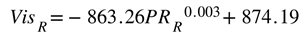
Figure 4(a) and Figure 4(b) respectively show image frames from VTD simulation without rain and with rain. By analyzing these image frames alone, the differences in corruption are not very noticeable except for the presence of raindrops. The main reason for this is that in real-world rainy conditions, there is not only the influence of raindrops but also the decrease of visibility. To better simulate real-world rainy conditions, we utilized the formula proposed in [38–40] to calculate the corresponding visibility for a specific rainfall rate.
When the rainfall rate exceeds 7.6 mm/h or higher, you can calculate the corresponding visibility using Equation (1). This will provide the visibility corresponding to different rainfall rates, where represents the rainfall rate, and represents the visibility. In this way, you can set rain parameters like those in Table 1 and calculate the corresponding rain visibilities. For instance, for rain rates of 43~48 mm/h, the corresponding visibility is approximately 300~200 meters, as shown in Table 4. Figure 4(b) demonstrates that by simulating rain alone without including the visibility effect of rain in VTD, compared to calculating corresponding visibilities for different rain rates and resetting weather parameters to include rain with visibility influence, the simulated rainy image frames closely resemble real rainy scenarios, as depicted in Figure 4(c). This method allows for the quantification of parameter adjustments for different severity levels, enabling users to rapidly configure various weather parameters and test scenarios. When combined with the automated test scenario generation tool, it becomes possible to efficiently generate more realistic weather-related scenario-based test benchmark using the VTD simulation tool.
3.2.2. Noise-Related Corruptions
In addition to being affected by weather-related factors that impact reliability and robustness, self-driving perception systems may also be susceptible to various image noise corruptions. Examples of such image noise corruptions include single pixel defects, column pixel defects, and cluster pixel defects, which can potentially lead to object detection failures. To facilitate comprehensive testing and validation, we have developed an image noise injection tool. This tool allows for the quantification of parameters to adjust different types of image noise and corruption percentages, thereby generating image noise corruptions of varying severity.
Furthermore, apart from the image noise corruptions caused by the camera itself, some cameras used in self-driving perception systems or advanced driver assistance systems are mounted behind the windshield of the vehicle. Consequently, when vehicles operate in rainy conditions, numerous raindrops adhere to the windshield, resulting in corruption with the camera's view. The size of these raindrops varies, and the density of raindrops differs under various rainfall rates. Investigating how raindrop corruption affects the reliability and robustness of object detection under different rainfall intensities is also a focal point of this research.
As illustrated in Figure 5, we utilize the VTD simulation platform in conjunction with an automated test scenario generation tool to generate image frames without weather corruption. Subsequently, we input these original clean image datasets into our developed image noise injection tool, or an artificial raindrop generation tool built on the Unreal Engine platform. This enables us to create image datasets with quantifiable adjustments to corruption severity or varying raindrop sizes and densities under the same test scenarios.
Figure 6(a) displays an image frame with clear blue skies and no image noise corruption, where the object detection model accurately identifies and labels each vehicle object. However, in the presence of image noise corruption and using the same object detection model, it is evident that several vehicles cannot be successfully identified, potentially causing a failure in the self-driving perception system, as depicted in Figure 6(b). Conducting a significant number of tests with various levels of camera image noise corruption during real-world autonomous driving validation is challenging and does not allow for controlled adjustments of different image corruption types and severity levels. Therefore, to enhance the test coverage of autonomous driving perception systems, we must be able to test and analyze the robustness and reliability of object detection models under different image noise corruption conditions.
To make it easier for users to generate image noise corruption, all that's required is to configure the original clean image data and specify the type of image noise to be injected. Users can also set different percentages of image noise corruption. Once this configuration is prepared, it can be imported into the image noise injection tool. The tool then randomly selects pixel positions in the images based on the specified corruption type and percentage and injects noise into those positions. It ensures that the pixel errors meet the specified percentage requirements, allowing for the rapid creation of various image noise datasets. Figure 7 illustrates the configuration parameters for different types of image noise corruption and severity regions. The six types of image noise corruption include Hot pixel defect, Single pixel defect, Column pixel defect, Cluster 2×2 pixel defect, Cluster 3×3 pixel defect, and Cluster 4×4 pixel defect.
3.2.3. Raindrop factor
To achieve a more realistic effect of raindrops hitting the windshield and interfering with the camera's image, we must consider the impact of different rainfall intensities and raindrop properties [34]. The severity of corruption caused by raindrops on the camera installed behind the vehicle's windshield depends primarily on three parameters: raindrop density, raindrop size, and raindrop velocity. However, the most significant factor influencing these three parameters is the rainfall intensity.
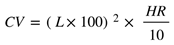
Assuming there is a 10-meter cubic structure, the rate of accumulating rainwater capacity varies under different rainfall intensities. We can calculate how many milliliters of rainwater can accumulate in the cube in one hour for different rainfall intensities using formula (2), where CV represents the hourly accumulated volume of rainwater in the cube (milliliter), HR represents the rainfall intensity (mm/h), and L represents the side length of the cube (m).
Next, based on the research findings from references [23–25], we estimate the approximate raindrop diameters corresponding to different rainfall intensities. When the rainfall intensity is greater, the raindrop diameters tend to be larger. Different raindrop diameters not only affect the raindrop's volume but also influence the speed at which raindrops fall [35]. Assuming the accumulated rainwater capacity in the cube remains constant, the raindrop diameter will affect the total number of raindrop particles that accumulate in one hour. Additionally, the raindrop's falling speed will impact how many raindrop particles interfere with each camera image.
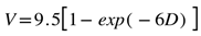
Assuming a raindrop falling height of 20 meters, we can calculate the raindrop's falling speed relative to different raindrop diameters using formula (3) proposed in paper [39], where V represents the raindrop's falling speed, and D represents the raindrop's diameter.
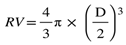
To calculate the rainwater capacity accumulated in a 10-meter cubic structure within one hour, along with the corresponding raindrop diameters and the number of raindrop particles, we first use formula (4) to compute the raindrop volume associated with raindrop diameter. In this formula, RV represents a raindrop volume, and D represents the raindrop diameter. Next, we can use formula (5) to estimate approximately how many raindrops fall into the cubic structure per hour.
The distance between the camera installed behind the windshield of the vehicle plays a role in the number of raindrops captured in the image when the raindrop density remains the same. When the camera is positioned farther away from the vehicle's windshield, the number of raindrops falling on the image will be greater. Conversely, if the camera is closer to the windshield, the number of raindrops captured in the image will be lower. Therefore, to accurately represent raindrop corruption in the camera's image, we must consider the distance between the camera and the vehicle's windshield.
However, the camera installed behind the vehicle's windshield captures only a small portion of the windshield's total area. The actual size of the windshield area captured by the camera depends on the distance between the camera and the windshield. This area is significantly smaller compared to the area of the 10-meter cube. The number of raindrops falling on the portion of the windshield captured by the camera in one second can be calculated by expression (6). Then, based on the camera's frame rate (fps), we can compute the average number of raindrops landing in each frame by expression (7). Consequently, we can achieve a more realistic representation of raindrop corruption in the simulation experiments.
Different raindrop sizes result in distinct shapes when they land on the windshield. To simulate more realistic raindrop shapes, we drew inspiration from the various-sized real raindrop shapes presented in paper [36] and proposed raindrop models tailored to our simulated environment, as depicted in Figure 8. The high similarity between our simulated raindrop models and real raindrops is evident in Figure 8.
Table 5 outlines the raindrop volume size range covered by different raindrop models. However, it's important to note that within the same model, different raindrop sizes may not have identical shapes. Therefore, we first select the appropriate raindrop model based on raindrop volume, as indicated in Table 5. Then, using formula (8), we calculate the scaling factor of the model to zoom in or zoom out the raindrop to produce any size of the raindrops. In this formula, Raindropvolume represents the raindrop's volume size, and Modelvolume represents the volume of the selected raindrop model. This approach enables us to scale the raindrop models within the UE4 simulation platform to generate different raindrop sizes that closely resemble real raindrop shapes, thereby enhancing the reliability of our testing and validation.
In the real scenario of rainfall, as more raindrops fall on the windshield of a car, the initially stationary raindrops on the windshield may coalesce with other raindrops. When they reach a certain size, they will flow down the windshield instead of remaining in a fixed position. Therefore, in our raindrop generation, we have incorporated a continuous model to calculate the size of each raindrop coalescing on the windshield. When the raindrops reach a size sufficient to flow down the windshield, we simulate the image frames of raindrops descending. Through this tool, we can generate a dataset of raindrop corruption images corresponding to different rainfall intensities.
In contrast to the raindrop generation tool proposed in [37], our method, utilizing the UE4 simulation platform for raindrop generation, takes approximately 0.833 seconds per frame to generate raindrop corruption images. This represents a significant improvement in the efficiency of generating raindrop corruption image datasets compared to the approximately 180 seconds per frame required by the method described in the literature.
3.3. Safety-Related Corruption Similarity Filtering Algorithm
Currently, there is no clear specification outlining the testing criteria for the benchmark test set of autonomous vehicle perception systems, nor is there any research team or organization that can guarantee that the test items included in a self-designed benchmark test set encompass all possible corruption factors. Given the highly complex driving environment that autonomous vehicle perception systems face, most study indicates that a higher number of test items results in better test coverage. However, continually expanding the test items to include a large number of repetitive or similar testing scenarios can lead to excessively long testing time, thereby increasing testing complexity and costs. Likely, if reinforcement training of object detection models includes many repetitive or non-critical scenarios, such a training not only consumes significant time but also cannot ensure that the robustness or overall performance of object detection model will be effectively enhanced to a substantial extent. This can impose a significant impact on the development timeline for autonomous driving, and waste the time and resources invested.
In response to the aforementioned issues, this work proposes a safety-related corruption similarity filtering algorithm to effectively reduce the number of test items while maintaining a high level of test coverage. Figure 9 illustrates the overlapping analysis procedure and corruption filtering concept among n corruption types denoted as C1 ~ Cn. In the beginning, we adopt previously introduced scenario generation methods for weather-related, noise-related and raindrop corruptions to construct two datasets: a benchmark testing dataset and a training dataset. The establishment process is as follows: we select two sets of corruption-free (or clean) dataset, both originating from the same environmental context, such as a city environment, but with distinct testing scenarios and traffic participants. One clean dataset is used to generate image datasets with n different corruption types for training purpose and similarly the other clean dataset is used for benchmark testing usage, as depicted in Figure 9(a) and Figure 9(b). The dataset marked as Ci, i = 1 to n, as shown in Figure 9(b), represents a dataset with Ci corruption type.
Subsequently, we select an AI object detection model and conduct transfer learning using this model in conjunction with training datasets containing various corruptions. The number of trained models equals the total number of different corruption types, plus one standard model trained using a clean dataset without any corruption, referred to as the Standard model. Apart from the Standard model, the remaining object detection models are trained using a single type of corruption, along with a clean dataset, for transfer learning. Ultimately, we obtain n distinct object detection models trained for different corruptions, denoted as M1 ~ Mn, in addition to the standard model, as illustrated in Figure 9(b).
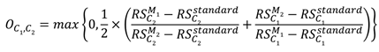
Figure 9(c) illustrates the overlap scores between pairs of corruption types. These scores are used to analyze the degree of correlation between two different corruptions, with higher overlap scores indicating a higher degree of similarity between them. We employ the overlap score calculation method proposed in paper [38]. First, we define the robustness score (RS) of model m for corruption type CT as shown in equation (9), where Aclean represents the detection accuracy of the model on an uncorrupted test dataset, and represents the detection accuracy of the model on the same test dataset corrupted by a specific corruption type CT. Equation (9) quantifies the model's robustness performance under a specific corruption type, where a lower score indicates insufficient robustness of the model to this corruption type, necessitating improvement. Equation (10) provides the formula for calculating the corruption overlap score between two different corruptions, C1 and C2. Here, "standard" and" M1," " M2" represent the selected model using an uncorrupted training dataset and the same training dataset with data augmentation of C1 and C2, respectively. The score in Equation (10) ranges between 0 and 1, with a higher score indicating a greater overlap and similarity between C1 and C2. According to Equation (10), we can construct a two-dimensional corruption overlap score table, denoted as overlap score OS(NC, NC), where NC represents the number of corruption types. OS(i, j) represents the overlap score between corruption type i and corruption type j.

| Algorithm 1: Corruption Similarity Filtering Algorithm |
|
Input: given a two-dimensional overlap score table OS(NC, NC) where NC is the number of corruptions and OS(i, j) represents the overlap score between corruption i and corruption j. Set up an overlap threshold θ to guide the filtering of corruptions from the overlap score table. Output: a subset of NC corruptions which will be used to form the benchmark dataset k ← NC
|
Next, we propose an effective corruption similarity filtering algorithm as described in Algorithm 1, based on the given overlap score table OS(NC, NC) and an overlap threshold, to identify a minimal set of corruption types where the correlation between these corruption types is less than the specified overlap threshold. Using the filtering algorithm, Figure 9(d) shows the corruption type results after the algorithm with NC=9. For example, with an overlap threshold set to X1, 0< X1<1, the algorithm retains three representative corruption types: C1, C2, and C5. This means that under the overlap threshold X1, C1 can represent C3, C4, and C6 because the overlap scores OS(C1, C3), OS(C1, C4), and OS(C1, C6) are all greater than or equal to the overlap threshold X1. Similarly, C2 and C5 are two other representative corruption types. In this demonstration, nine corruption types are partitioned into three corruption groups as shown in Figure 9(d), and C1/ C2/C5 are representative corruption types for group 1/2/3 respectively. The choice of the overlap threshold will affect the number of eliminated corruption types. Clearly, a lower threshold will result in the smaller number of corruption types remained after the filtering algorithm.
Through this algorithm, we can set the overlap threshold based on different levels of testing requirement and then use the representative corruption types after filtering to construct the benchmark testing dataset, as shown in Figure 9(d). Figure 9(d) illustrates the presence of three distinct types of benchmark testing datasets: B1, B2, and B3. Here, B1, B2, and B3 represent single-corruption, two-corruption, and single-corruption plus two-corruption induced scenarios, respectively. The filtering algorithm allows for the removal of similar corruption types, reducing the number of corruption types to consider. This can lead to a shorter testing and validation time for object detection models and can also be used to evaluate the quality of the benchmark testing dataset, ensuring that the required test coverage is achieved within a shorter testing time.
To utilize the corruption similarity filtering algorithm, you must provide a two-dimensional overlap score (OS) matrix data, and configure the overlap threshold θ. This threshold guides the algorithm in filtering relevant corruption types. Ultimately, the algorithm will produce the filtered corruption types, which are representative and used for constructing training and benchmark testing datasets. The main objective of corruption filtering algorithm is to find the smaller number of corruption types to represent the original set of corruption types. This process ensures a reduction in training and testing time cost while still maintaining the efficient coverage and quality. It is particularly beneficial during the early stages of perception system design as it accelerates the development speed. Corruption grouping algorithm presented in the following Algorithm 2 is developed to find the corruption groups as shown in Figure 9(d). The main concept of corruption grouping algorithm is to use the filtered corruption types derived from the corruption similarity filtering algorithm, and for each filtered corruption type to discover the other members of the corruption group.
| Algorithm 2: Corruption Grouping Algorithm |
|
Input: given a two-dimensional overlap score table OS(NC, NC) where NC is the number of corruptions and OS(i, j) represents the overlap score between corruption i and corruption j. Set up an overlap threshold θ. Output: corruption groups
|
By adjusting overlap threshold, the number of retained corruption types after filtering will vary, leading to different testing and validation time for object detection models. Equation (11) can be used to calculate the time required for testing and validation with different benchmark testing datasets. The explanation is as follows: define NI as the total number of image frames in the original corruption-free dataset. Through the corruption filtering algorithm, the number of retained corruption types is denoted as k. Corruption types are represented as Ci, where the range of i is from 1 to k. Each corruption type Ci has a different number of severity regions, defined as NSR(Ci). Benchmark 1 (B1) is single-corruption induced scenario dataset which is constructed by the following method: we first need to generate single-corruption induced scenarios for each corruption type, and then collect all single-corruption induced scenarios created for each corruption type to form the B1. Each severity region within a corruption type uses the original corruption-free dataset to generate its single-corruption induced scenarios, and therefore, there are NSR(Ci) sets of single-corruption induced scenarios for corruption type Ci. As a result, we can see that the testing time for each corruption type is the result of multiplying NSR(Ci), NI, and DTm. Here, DTm is defined as the estimated time it takes for the object detection model m to recognize a single frame, allowing us to calculate the overall testing and validation time BTTm using Equation (11).
3.4. Corruption Type Object Detection Model Enhancement Techniques
The robustness of object detection models in autonomous driving perception systems can be enhanced by conducting model transfer learning using datasets that incorporate various corruption types proposed in this study. However, utilizing datasets with a wide range of corruption types also incurs significant time and cost for model training. After reducing corruption types with high similarity through filtering algorithms, we can proceed with model enhancement training using the remaining corruption types. This approach helps to reduce the time required for model enhancement training.
The calculation of the time required for model enhancement training using corruption type image datasets is represented by Equation (12). Here, we define NEC as the number of corruption types to be enhanced, and the enhanced corruption types used are denoted as ECi, where i ranges from 1 to NEC. Additionally, for each corruption type, the number of severity regions for each enhanced corruption type is defined as NER(ECi), and the regions for each enhanced corruption type are denoted as ECi(Rj), where j ranges from 1 to NER(ECi). The number of images used for model enhancement training is NEI.
In Equation (12), the number of images required for each severity region of each corruption type is NEI, and the number of input images for each step of the model enhancement transfer learning is IS. The estimated training time for each step of the model transfer learning is ETm. The total number of epochs for model enhancement transfer learning is NE. Finally, using these parameters, we can calculate the total training time METm required for enhancing object detection model m.
It is expected that by training representative corruption types within each corruption group, the robustness of each corruption type within the group can be improved. As shown in Table 6, there are two different training approaches for object detection models. The first approach uses the corruption filtering algorithm to remove corruption types with high similarity and then employs the retained corruption types to enhance the model. The second approach involves training the model using all original corruption types, which requires the most training time. In the testing dataset, we categorize it into four types. The first type is the original baseline testing dataset, which includes test image data for all corruption types, resulting in the longest overall testing time. The second type uses the filtered corruption types to represent the original corruption types, reducing the overall testing time compared to the original baseline testing dataset. The third and fourth types involve using a filtering algorithm to reduce high-similarity corruption types, creating two corruption groups: (Fog & Rain) and (Hot, Single, Cluster 22/33/44). Within these groups, specific corruption types (e.g., Fog and Cluster 22) represent their respective corruption groups. The idea behind filtering is to reduce the number of corruption types to simplify training and testing.
We then need to verify the effectiveness of the reduced corruption types from the aspect of the training and testing processes. Table 6 presents a comparative analysis of different training datasets for object detection models on various testing datasets. The real experimental results will be provided in Section 4. Here, we employ this table to explain the goals of our approach trying to achieve. In Table 6, the difference between A and C indicates the training effectiveness of filtered corruption types. The smaller gap of (A, C) means that our proposed approach can effectively reduce the model training time and meanwhile maintain the model quality compared with the model trained by all original corruption types. Similarly, the difference between A and B indicates the effectiveness of test dataset built by filtered corruption types. The smaller gap of (A, B) signifies that the testing dataset formed by filtered corruption types can still maintain good testing coverage while significantly reducing testing time. Next, when value E approaches G, it indicates that using the fog corruption type to represent the (Fog & Rain) corruption group has a good effect. Similarly, when value F approaches H, it signifies that using the Cluster 22 corruption type to represent the (Hot, Single, Cluster 22, 33, 44) corruption group has an excellent effect.
In real-world driving scenarios, it is common for multiple corruption types to occur simultaneously, such as rain and heavy fog. This study aims to analyze and investigate how the simultaneous occurrence of two different corruption types affects the model's detection performance. It is essential to consider that when dealing with a huge number of corruption types, each having various severity regions and subregions, the resulting dataset can become extensive and complex. As shown in Table 7, if we have already applied a filtering algorithm to remove highly similar corruption types and left with two corruption types: fog and cluster 22. The object detection model has been tested and validated separately for each of these two corruption types. Using the testing data, we can analyze which severity region within a specific corruption type yields the poorest detection performance. This analysis is referred to as the model's vulnerability analysis. For instance, if the model performs poorly in the fog corruption type's severity region with visibility ranging from 50 to 20 meters, it indicates that this region requires special training to enhance the model's robustness. Similar vulnerability points can be identified for cluster 22 corruption type.
Next, we take the vulnerability region of the fog corruption type to determine the midpoint of the visibility region, i.e. 35 meters and redefine two severity subregions: SR1 (visibility ranging from 50 to 35 meters) and SR2 (visibility ranging from 35 to 20 meters). These two subregions can be used to define the severity setting for combinations of the fog corruption type with other corruption types. We can then create the possible enhanced training datasets for the combinations of the fog & cluster22 corruption types and conduct model transfer learning. Looking at Table 7, for example, the combination of fog & cluster 22 can result in four possibilities: (42.5m, 13.5%), (42.5m, 14.5%), (27.5m, 13.5%), and (27.5m, 14.5%). This approach is expected to effectively reduce the size of the training dataset for two-corruption induced scenarios while maintaining good coverage. Training the model with these two corruption type combinations can enhance its detection performance when both corruption types occur simultaneously.
As shown in Table 8, we want to compare and analyze the robustness performance of four different models on Benchmark 1 (B1) with single-corruption induced scenarios and Benchmark 2 (B2) with two-corruption induced scenarios. The real experimental results will be given in Section 4. Here, we depict the idea of the comparisons. First is the Model-Clean object detection model, which undergoes transfer learning without any corruption, and is expected to have the lowest performance among the four models. Next is Model-B1, which uses filtered corruption types to produce the single-corruption training dataset for enhanced training. Then according to the filtered corruption types, Model-B2 adopts two-corruption induced training data to enhance model detection performance. Finally, for Model-Original, which undergoes enhanced training using all corruption types, significant training time is required. If the experimental results E-1-1 and E-2-1 are similar to E-A-1, it indicates the effectiveness of the filtering algorithm proposed in this study, as it can maintain good system robustness in a shorter training time. Considering that real-world traffic situations may involve the simultaneous occurrence of two corruption types, it is necessary to investigate their impact on the model. Thus, besides conducting single corruption type testing and validation, it is essential to perform testing and validation on benchmark B2, which comprises two corruption type combinations, to ensure that the model's robustness meets system requirements.
Therefore, we will analyze whether Model-B1 and Model-Original, trained using only one corruption type in the enhanced training dataset, can maintain good robustness performance in B2 with two corruption type combinations. Conversely, training the model with two corruption type combinations may yield good performance in B2, but it remains to be seen whether it can also demonstrate strong robustness performance in B1. The next section will provide further analysis and discussion of the experimental results. Ultimately, we hope that these experimental results will assist designers in finding a suitable solution based on model testing and enhancement training time considerations.
4. Experimental Results and Analysis
4.1. Corruption Types and Benchmark Dataset Generation
This work is based on the VTD vehicle simulation platform and demonstrates two of the most common driving scenarios: city roads and highways. Two city road scenarios and two highway scenarios were created. The recorded video footage was captured using cameras installed on the windshields of simulated vehicles, with a resolution of 800 × 600 pixels and a frame rate of 15 frames per second (FPS). These recordings were used to create benchmark test datasets and model enhancement training datasets. In total, there were 5,400 original, unaltered video frames for the city road scenarios and 3,840 for the highway scenarios.
As shown in Table 9, we utilized the weather-related, and noise-related generation tools proposed in this study to demonstrate the robustness and performance testing of object detection models under nine different corruption types. The weather corruption types include fog and rain. There are a total of five severity regions for fog, with visibility ranging from 200 to 20 meters. In the case of rain corruption, there are two severity regions, with rainfall ranging from 43 to 54.8 mm/h, resulting in approximately 300 to 100 meters of visibility. Noise corruption types comprise seven categories: hot pixel defect, single pixel defect, cluster 22/33/44 pixel defect, column pixel defect, and raindrop corruption. Among these, raindrop corruption is configured with two severity regions, including rainfall rates of 20-50 mm/h and raindrop diameters of 0.183-0.229 cm. The remaining noise corruption types are set with three severity regions, and the range of image noise corruption is 1-15%.
We started by generating two original, corruption-free image datasets using the VTD simulation platform: one for city scenes and the other for highways, each containing 5400 images. The benchmark testing dataset includes datasets for all individual corruption types and severity regions. For the complete benchmark testing dataset, we generated datasets with corruption for each corruption type and severity region by using weather and noise-related corruption generation tools on the original, corruption-free image dataset. Overall, we demonstrated a total of nine different corruption types, along with an image type with no corruption. As mentioned before, each severity region in a corruption type needs 5400 original, corruption-free images to create single-corruption induced scenarios. Therefore, the total number of images for the city and highway original benchmark testing datasets is 5400 images × 28 = 151,200 images, respectively.
As displayed in Figure 10, using the VTD simulation combined with the weather and noise-related generation tools, we can clearly observe that as severity increases, the corruption in the images also significantly increases. Users can quantitatively adjust severity to generate benchmark testing image datasets with varying degrees of corruption. This capability helps improve test coverage for rare adverse weather or noise corruption scenarios, ensuring that the system's reliability and robustness meet requirements.
4.2. Corruption Type Selection
Due to the differences between city and highway scenarios, such as the presence of various buildings and traffic participants in city areas, as opposed to the relatively simpler highway environment, the performance of object detection models in autonomous driving perception systems may vary. The reliability and robustness of these models under different scenarios and corruption types may also differ. Therefore, we present experimental demonstrations in both city and highway scenarios. We use the "faster_rcnn_resnet101_coco" pre-trained model provided in the TensorFlow model zoo, employing corruption filtering algorithms and adjusting different overlap threshold parameters to remove corruption types with high similarity. We then compare and analyze the differences in filtered corruption types after filtering in the city and highway scenarios.
As illustrated in Figure 11, the experimental results of the overlapping scores for all corruption types in city and highway scenarios reveal that two corruption types, "fog" and "rain," exhibit high similarity in both scenarios. However, the similarity of these two corruption types with other corruption types is significantly lower. Furthermore, the "raindrops" corruption type also shows a considerable dissimilarity with other corruption types. In addition, it is evident that there are differences in the overlapping scores between the two scenarios, especially in the case of the "noise" corruption category. We observed another interesting point that the overlapping score between "raindrop" and "column" corruption types is 0.38 in the highway scenario, whereas it is zero in the city scenario. This variation may be primarily attributed to the traffic environment of the city and highway scenarios. Therefore, it is necessary to conduct separate testing and validation analyses for different categories of scenarios to assess the impact of different corruption types and their severity.
Figure 12 and Figure 13 show filtered corruption types in city and highway scenarios with different thresholds. For city scenarios, the thresholds were 0.4 and 0.6, resulting in three and four filtered corruption types, respectively. For highway scenarios, the thresholds were 0.4 and 0.5, also yielding three and four filtered corruption types, respectively. In the city scenario, with an overlap threshold of 0.6, corruption types were reduced to four, which included "fog," "cluster 22,", "raindrop", and "column". While threshold reduces to 0.4, column corruption was removed, leaving the other three corruption types unchanged. On the other hand, in the highway scenario, we obtain the same filtered corruption types with the city scenario while setting overlap thresholds at 0.4 and 0.5.
After performing the filtering similarity corruption algorithm, the corruption grouping algorithm based on the filtering results was used to acquire the corresponding corruption groups. Figure 14 exhibits the corruption groups formed by different thresholds in city and highway scenarios. For threshold at 0.4, the first group includes two corruption types: "fog" and "rain," with "fog" representing this group. The second group comprises six corruption types: "hot pixel," "single pixel," "cluster 22/33/44," and "column", with "cluster 22" as the representative corruption type. The third group consists of only one corruption type, "raindrop". For city threshold at 0.6 and highway threshold at 0.5, the only change is in the group represented by "cluster 22", where the "column pixel" corruption becomes a separate group.
4.3. Model Corruption Type Vulnerability Analysis and Enhanced Training
If the object detection model is trained with less severe or almost non-impactful data or if it uses a dataset that includes all possible corruption types and severity regions, it may consume a significant amount of training time and data space, with limited improvement in overall model robustness. Concerning about the effectiveness of the training process for the models, we propose an approach based on the corruption type vulnerability analysis to discover the severity region which has the most significant impact on the accuracy of model for the considered corruption types. The main objective of this approach is to identify the severity region with the highest impact on the model for each corruption type. Subsequently, we can propose an appropriate enhanced training dataset for the vulnerability region of each filtered corruption type and perform transfer learning. In this way, the size of the enhanced training dataset and the time required for model training can be reduced significantly, and meanwhile, we can efficiently improve the model robustness for the considered corruption types.
We use an example as shown in Table 10 to explain how to identify the vulnerability region for a corruption type. Table 10 lists nine considered corruption types C1 ~ C9 and according to Figure 13(b), C1 and C7 ~ C9 are the representative corruption types selected from the corruption filtering algorithm. In the ‘Fog’ corruption type, we vary visibility from 200 to 20 meters, with a difference of 30 meters between each severity level. This results in a total of seven different levels of severity (NSL). In the "Noise" corruption types, "Cluster22" and "Column", we set severity levels between 1% and 15%, with a 2% difference between each severity level, resulting in eight different levels of severity for each type. Finally, for the "Raindrop" corruption type, we vary rain quantity from 20 to 50 mm and raindrop diameter from 0.183 to 0.229 cm, resulting in three different levels of severity. Then, we create test datasets for the representative corruption types with severity levels shown in Table 10 in both city and highway scenarios. Therefore, the number of test datasets required for C1 and C7 ~ C9 are 7, 8, 8 and 3, respectively.
Next, we conduct the model test for each test dataset and analyze the slope variations of the different severity regions in terms of changes in object detection accuracy. The test results are exhibited in Table 11. As shown in Table 11, in this experiment, we utilized the faster_rcnn_resnet101_coco pre-trained model provided in the TensorFlow model zoo for object detection. Subsequently, we employed two distinct clean datasets: one representing city roads and the other representing highways. We first conducted transfer learning to develop two object detection models, namely city_clean and highway_clean models. Then, we proceeded to evaluate and compare the impact of different corruption types and severity levels on the city_clean and highway_clean models within the two distinct scenes. From the experimental results, it is evident that even though the corruption types tested in both city and highway scenes are the same, the model performs notably better in the highway scene. The primary reason for this discrepancy lies in the fact that the overall complexity of backgrounds in highway images is considerably lower compared to city road scenes. City roads are characterized by various buildings and diverse objects in the vicinity, leading to lower overall model detection accuracy. From Table 11, we observe significant differences in the object detection accuracy for the fog corruption type in both city and highway scenes. In the visibility range of 200m to 20m, the overall model Average Precision (AP) drops by 68.67% in city road scenes, while in the highway scene, the drop is only 49.06%. Specifically, under a severity level of 20 meters, the test results differ by as much as 32.56, highlighting the more pronounced and severe impact of fog corruption on the model in city road scenarios.
Within the same corruption type, we assessed the influence of different severity regions on the model's detection rate by analyzing the variation in detection accuracy with severity levels. For each corruption type and its respective severity regions, we calculated the slope of the variation in model detection accuracy and identified the severity region with the steepest slope. This region represents the model's vulnerability to that specific corruption type, indicating the area where the model requires enhanced training most. From Table 11, we see that the visibility region between 50m and 20m represents the severity region with the highest slope of change for fog in both city and highway contexts. For the other three corruption types, their influence on object detection in city and highway scenes is less pronounced than fog. From the experimental results, it becomes evident that different corruption types affect the model to varying degrees. This insight allows us to identify which corruption types require special attention in terms of enhancing the model's detection capabilities. In city road scenes, the severity regions with the most significant impact for Column and Cluster22 corruption types are 13% to 15%, and for Raindrop corruption, it is 20mm to 35mm/h. In the highway scenario, except for Column corruption, which has a severity range of 1% to 3%, the chosen severity regions for other corruption types are the same as those in the city scene. Subsequently, based on the identified vulnerability regions for corruption types, we propose the enhanced training dataset to conduct transfer learning to improve the model robustness. This approach effectively improves the model's robustness and meanwhile reduces the training time cost.
The construction of the scene for enhanced training dataset was carried out using the VTD simulation platform, where city and highway scenarios were established. The simulation was configured to generate 15 frames per second, resulting in a total of 3,840 frames for each scenario. Additionally, weather conditions and image noise, along with a raindrop generation tool proposed in this research, were used to generate training datasets for each corruption type with their respective vulnerability regions. Furthermore, within the dataset for model enhancement and transfer learning, we divide it into two benchmarks: Benchmark 1, focusing on the enhancement training of a single corruption type, and Benchmark 2, which combines two corruption types for training. To prevent the issue of model forgetting during training, we incorporate a set of clean images, not affected by any corruption, into each dataset. This helps ensure that the accuracy of object detection for objects unaffected by corruptions is not compromised.
We performed a comparative analysis of the robustness performance in city and highway scenes using different enhanced training datasets for model transfer learning. Based on the publicly available pre-trained model, the faster_rcnn_resnet101_coco model provided in the TensorFlow model zoo, which we refer to as M1 object detection model. The hyperparameters of training process for transfer learning is depicted as follows. The number of input images per step (IS) was fixed at two, the total number of epochs (NE) for model enhancement transfer learning was set to 8, and the experiment was conducted on a computer equipped with an Intel i5-10400 CPU, DDR4 16GB RAM, and a GeForce RTX™ 3060 GPU. The training time required for each step in the M1 model transfer learning, denoted as ETM1, is approximately 0.275 seconds. We then compared the training times and robustness improvements for different training datasets.
Table 12 shows the performance of our detection model in city and highway scenarios, undergoing reinforcement training for a single corruption type using four distinct reinforcement learning datasets. These datasets are described below.
- Dataset without any corruption.
- Dataset containing all corruption types with all severity regions.
- Dataset with three corruption types (F3) derived from the corruption filtering algorithm.
- Dataset with four corruption types (F4) derived from the corruption filtering algorithm.
We investigated the impact of different reinforcement learning datasets on the training time required for model training while maintaining the same training hyperparameters as given above. Relevant parameters are defined as follows:
- NEI: Number of images containing in an enhancement dataset.
- NEC: Number of enhancement corruption types.
- ECi: The i-th enhancement corruption type, where i=1 to NEC
- NER(ECi): Number of severity regions for enhancement corruption type i, where i is from 1 to NEC.
- ECi(Rj): The j-th region of enhancement corruption type i, where j = 1 to NER(ECi)
- For each severity region ECi(Rj), the number of reinforcement training images is denoted as NEI.
- IS: Number of input images for each transfer learning step.
- ET: Estimated the time of required for transfer learning in second per step for object detection model.
- NE: The total number of epochs for model reinforcement transfer learning.
- MET: The training time required for object detection model reinforcement.
The first training model, M1-Clean, uses only the clean training dataset without any corruption for reinforcement training. Here, NEI is 3840 images. The estimated training time for model reinforcement is calculated as. Since this model is trained solely with the clean dataset without any corruption, it requires the shortest time and the fewest training images. Therefore, M1-Clean serves as the baseline for evaluating the robustness of other reinforcement training models.
The second training model, M1-All, incorporates all corruption types and severity regions into the reinforcement training dataset. As shown in Table 10, there are a total of nine corruption types (NEC=9). The number of severity levels for NER(ECFog) is seven, while both NER(ECRain) and NER(ECRaindrop) have three severity levels each. Finally, the corruption types Hot, Single, Cluster22/33/44, and Column all have eight severity levels. In total, there are 61 severity levels for all corruption types. Therefore, the total number of images in the reinforcement training dataset including the clean type is . The estimated training time for this model is , making it the model with the highest number of reinforcement training images and the longest training time among the four models. The third and fourth training models, M1-B1F3 and M1-B1F4, were created based on the enhanced training dataset generated from the vulnerability regions of the representative corruption types. Both city and highway scenes have the same set of representative corruption types, with a total of 3 corruption types (NEC=3) for M1-B1F3 and 4 corruption types (NEC=4) for M1-B1F4. Therefore, the estimated training time for M1-B1F3 and M1-B1F4 are and respectively. Overall, the required training time for M1-B1F3 and M1-B1F4 is significantly reduced compared to M1-All.
As depicted in Table 12, the four reinforcement training datasets not only differ significantly in the number of images but also show a substantial difference in the estimated training time for model reinforcement transfer learning, especially the M1-All model, which is trained with all corruption types and severity levels. The overall training time for M1-All is much higher compared to models that have reduced corruption types (M1-B1F3 and M1-B1F4). We note that blindly increasing the number of training images without a proper selection strategy can lead to a sharp increase in training time. On the other hand, if additional reinforcement training data consists of non-severe or less impactful datasets, it may incur significant training costs and time without substantial improvements in the robustness of the object detection model. The issue of how effective of M1-B1F3 and M1-B1F4 compared to M1-All model will be discussed in the following subsection.
4.4. Robustness Analysis of Enhanced Training Models
Table 13 and Table 14 show the experimental results of Table 6 described previously. Four different test datasets were used for assessing robustness, where the assessment method involves summing and averaging the average precision (AP) scores of individual corruption types. The first test dataset comprises all corruption types plus the clean dataset, and the models were tested individually for each corruption type, followed by summing and averaging the AP scores. The results indicate that the object detection model trained with representative corruption types closely resembles the model trained with all corruption types. In the city scenario of Table 13, the two models exhibit AP scores of 75.8% and 75.06%, differing by only 0.74%. Similarly, in the highway scenario, the two models have very similar AP scores of 89.38% and 88.55%, with a difference of 0.83%. Table 14 presents the similar results. This demonstrates that the corruption filtered algorithm proposed in this study effectively reduces training time by removing highly similar corruption types while maintaining high training coverage. As a result, it achieves similar robustness to models trained with all corruption types.
The second test dataset was constructed from the representative corruption types plus the clean dataset. To objectively assess the robustness performance of these test datasets, the AP scores were calculated based on the group's representative corruption type's AP score, multiplied by the number of corruption types in that group, and then summed and averaged. This method enables a fair comparison between the test datasets formed by representative corruption types and all corruption type test dataset. As can be seen from Table 13, the results between the test datasets formed by representative corruption types and all corruption type test dataset are very similar for City_M1-B1F3, and highway_M1-B1F3 possesses the same phenomenon. It indicates that test dataset formed by representative corruption types maintains a similar test coverage to all corruption type test dataset. Besides, we observe the similar results in Table 14.
Another interesting point to be explored is the impact of setting overlap threshold values on the number of representative corruption types and the coverage of model training and testing. In both city and highway scenarios, the models M1-B1F3 and M1-B1F4 exhibit highly similar robustness performance on all corruption type test dataset. In this context, three representative corruption types are sufficient to cover all considered corruption types, and adding a fourth corruption type, such as Column corruption, does not provide any significant improvement. The third and fourth test datasets in Table 13 and Table 14 were built by corruption groups. These test datasets can be used to verify how effective of the representative corruption type to represent its corresponding corruption group. The results between x_M1-B1Fy, where x = City or Highway, y= 3 or 4, and M1-All for the third and fourth test datasets exhibit the effectiveness of the representative corruption type to represent its corresponding corruption group. For example, the data shown in the third test dataset of Table 13 (a) are almost identical and it means that the fog corruption can represent the rain corruption very well. Similarly, data shown in the fourth test dataset indicate that cluster22 also represents its corresponding corruption group well. In summary, according to Table 13 and Table 14, we can assure that the fog and cluster 22 can represent their corresponding corruption groups well. Consequently, we can achieve the good training and test coverage with lower training and test time cost.
4.5. Exploring Scenarios with Two Corruption Combinations
In real-world scenarios of autonomous vehicles, besides being affected by a single type of corruption, there are often situations where two different corruption types occur simultaneously, such as rain and fog occurring together. Therefore, we should further investigate the model's robustness performance in scenarios where two corruption types are combined. To simplify the experiments, we used three representative corruption types in city and highway scenarios to create reinforcement training datasets for M1-B2F3 model. As shown in Table 7 and Table 15, we divided the severity regions of corruption types into two sub-regions, denoted as SR1 and SR2. SR1 and SR2 sub-regions are represented by the severity data as described in Table 15, indicating the severity level of that corruption type's sub-region. There are three pairs of two-corruption combinations, including (Fog & Cluster22), (Fog & Raindrop), and (Cluster22 & Raindrop). To simplify the demonstration, the training datasets of two-corruption type combinations for (corruption type 1, corruption type 2) only consider the combinations of [corruption type 1 (SR1), corruption type 2 (SR1)] and [corruption type 1 (SR2), corruption type 2 (SR2)] as shown in Table 15. However, we also can follow the combinations described in Table 7 to increase the coverage of training.
For each two-corruption type combination, we generated its reinforcement training dataset using the following method: we used the original corruption-free image dataset, with the first half of the images generated with the SR1 severity combination from Table 15 to introduce two-corruption induced scenarios, and the second half of the images generated with the SR2 severity combination to introduce two-corruption induced scenarios. For example, in the case of the Fog & Cluster22 combination, the first half of the image dataset was created with a severity combination of 42.5m+13.5%, and the second half was produced with a severity combination of 27.5m+14.5%. The reinforcement training datasets for the two-corruption type combinations required images, and the test datasets for two-corruption combinations were constructed in the same manner.
Table 16 displays the performance of single and two-corruption type trained models in city and highway scenarios on single and two-corruption test datasets. From these data, it can be observed that the performance of model trained with two corruption types is slightly inferior to the single corruption type trained model on B1 single corruption test dataset and approximating the result of the M1-All model trained with all corruption types. All four models show a significant decrease in performance on the two-corruption test datasets, where the model trained with two corruption types outperforms the others. This suggests that in scenarios involving two-corruption type combinations, despite their lower occurrence probability, the testing of such combinations can reveal shortcomings in single corruption type trained models, highlighting the need for specific training on scenarios involving two corruption types to enhance the overall model robustness. This is an area that can be explored in future research.
4.6. Real-World Scenario Testing and Verification
In real-world driving environments for autonomous vehicles, the perception system may encounter adverse conditions or various potential corruptions, leading to system failures or anomalies. To improve the test coverage of these adverse scenarios or corner cases, in the experiments mentioned above, we generated datasets containing various weather and image noise corruption types using a vehicle simulation platform and developed the tools for generating scenario-based test datasets. The results of the experiments demonstrate that by identifying model vulnerabilities through the vulnerability analysis proposed in this study and building effective model vulnerability enhancement training datasets, the tolerance and robustness of object detection models to weather and noise-related corruptions can be significantly improved.
From the previous experimental results, it has been shown that the proposed robustness verification and enhancement approach can effectively improve the robustness of the detection models when tested against benchmark test datasets composed of various corruption types in simulated environments. To further confirm that object detection models trained through our method can perform well in real-world situations, we used the DAWN real-world adverse weather driving scenario dataset [39] and the Foggy Cityscapes real-world scene dataset with foggy weather as benchmark test datasets for real adverse driving scenarios to test our trained models. In the DAWN dataset, we excluded snowy corruption type that was not included in the experiments and the images with no vehicles. Additionally, for Foggy Cityscapes[40], we set the visibility parameter β to 0.08 to produce more severe fog with a visibility of approximately 37 meters in real-world scene datasets. Then, we can evaluate the robustness and reliability of models trained by simulated scenarios with these two real-world test datasets.
Table 17 presents the performance of four object detection models trained using different enhancement training datasets for city and highway scenarios. We observed that the models' robustness performance in real-world scenarios is significantly lower compared to the results obtained in virtual simulation environments, which is a common phenomenon in current virtual simulation environments. It should be pointed out that the model performance becomes very poor for Foggy Cityscapes test dataset because this test dataset was set under very severe fog condition. Our analysis here mainly focuses on the robustness verification and enhancement procedures proposed in this research, and how the models trained using the proposed methods perform in real-world scenarios. We note that the models trained by corruption-enhanced dataset indeed exhibit better robustness in real-world scenarios compared to models that have not undergone corruption-enhanced training.
From Table 17, we can observe that in city and highway scenarios, robustness performance of M1-B1F3 on the real-world test dataset is higher compared to the M1-Clean model. This demonstrates that the approach proposed in this research is indeed capable of improving the robustness of object detection models. We also found that the models trained in city scenarios exhibit better robustness performance compared to those trained in highway scenarios except M1-B1F3 model at DAWN test dataset. This is likely because city scenarios are more complex, leading to more effective training.
Besides, we adopted a strategy from reference [41] that involves incorporating a small amount of real image data for secondary transfer learning to enhance models further. This method has proven to be effective in enhancing the robustness of object detection models in real environments. Therefore, we introduced 800 images from the BDD dataset that were not affected by any corruption into both the M1-Clean and M1-B1F3 models. Subsequently, we performed secondary transfer learning and validated the models using two real-world benchmark datasets with adverse weather conditions. The experimental results clearly show that the M1-Clean_R800 and M1-B1F3_R800 models, trained with the addition of a small number of real data, can significantly improve the robustness compared to models trained using only simulated datasets. Particularly, the M1-B1F3_R800 model exhibits excellent improvement of robustness performance in adverse real-world weather conditions compared to models trained using only simulated datasets. Overall, the experimental results validate that the robustness verification and enhancement procedures proposed in this research can achieve good training and test coverage in both simulated and real-world environments for object detection models. Additionally, our approach can greatly reduce the time required for model enhancement training and validation. Through the various model enhancement schemes presented, designers can choose a suitable method for enhancing object detection models and conducting test verification with an efficient manner.
5. Conclusions
The design and test of autonomous driving systems require demonstrating their reliability and safety in any environment, especially when it comes to the robustness testing and verification of perception systems. Based on sensor-based perception systems, this study proposes a comprehensive method for robustness validation and enhancement using a simulation platform. We delve into issues related to test scenario coverage/effectiveness and scenario complexity (training and testing dataset sizes)/time efficiency. There are numerous factors affecting autonomous driving safety, and in this study, we focus on corruptions related to weather and noise, especially the corruption effects of single-corruption induced, and two-corruption induced scenarios on the robustness of autonomous driving perception systems. Given the complexity of single corruption and combinations of multiple corruptions in test scenarios and the substantial testing time required, it is essential to ensure the quality of test datasets and to conduct rapid testing and validation during the early stages of system development. Therefore, we propose an effective corruption filtering algorithm to reduce the number of considered corruption types to mitigate the complexity of test datasets and meanwhile maintain the good test coverage. We investigate the relationship between the parameter of "overlap threshold" in the corruption filtering algorithm and scenario complexity/time cost and test scenario coverage. This parameter setting affects the number of selected corruption types, the size of training and testing datasets, training and testing time, and test coverage rate. Through this analysis, an appropriate "overlap threshold" parameter value can be set to meet the requirements of effectiveness and economy, resulting in a set of optimal benchmark test datasets that satisfy time cost and test scenario coverage requirements. This ensures improving the test scenario coverage and effectiveness in less testing time.
To expedite the generation of benchmark datasets, we have developed the tools for generating simulated test scenarios dataset, which comprise weather-related test scenario generator and sensor noise injectors to emulate real traffic environments. We then utilize these benchmark datasets to test object detection models of perception systems. The model vulnerability analysis was performed to identify the fragile region of corruptions and create effective model vulnerability-enhanced training datasets to enhance the model's tolerance to weather and noise-related corruptions, thereby improving the perception system's robustness. We use case studies to demonstrate how to generate test scenarios related to weather (e.g., rain, fog) and noise (e.g., camera pixel noise) and perform robustness testing of the perception system using object detection models in these test scenario datasets. Then, the corruption similarity filtering algorithm was employed to identify the representative corruption types to represent all considered corruption types. Subsequently, we showcase the identification of vulnerability regions of representative corruption types and enhancement process using data augmentation techniques to generate effective training datasets for enhancing the robustness of the perception system. We further discuss the effect of two-corruption induced scenarios on the robustness of the models and leave the issue to be explored in future research. Finally, we verified our models trained in simulated environment with the real-word adverse test datasets to ascertain the effectiveness of our proposed approach.
References
- Min, K.; Han, S.; Lee, D.; Choi, D.; Sung, K.; Choi, J. SAE Level 3 Autonomous Driving Technology of the ETRI. In Proceedings of the 2019 International Conference on Information and Communication Technology Convergence (ICTC), October 2019; pp. 464–466. [Google Scholar]
- Klück, F.; Zimmermann, M.; Wotawa, F.; Nica, M. Genetic Algorithm-Based Test Parameter Optimization for ADAS System Testing. In Proceedings of the 2019 IEEE 19th International Conference on Software Quality, Reliability and Security (QRS), July 2019; pp. 418–425. [Google Scholar]
- Koopman, P.; Wagner, M. Autonomous Vehicle Safety: An Interdisciplinary Challenge. IEEE Intell. Transp. Syst. Mag. 2017, 9, 90–96. [Google Scholar] [CrossRef]
- Pezzementi, Z.; Tabor, T.; Yim, S.; Chang, J.K.; Drozd, B.; Guttendorf, D.; Wagner, M.; Koopman, P. Putting Image Manipulations in Context: Robustness Testing for Safe Perception. In Proceedings of the 2018 IEEE International Symposium on Safety, Security, and Rescue Robotics (SSRR), August 2018; pp. 1–8. [Google Scholar]
- Bolte, J.; Bar, A.; Lipinski, D.; Fingscheidt, T. Towards Corner Case Detection for Autonomous Driving. In Proceedings of the 2019 IEEE Intelligent Vehicles Symposium (IV), June 2019; pp. 438–445. [Google Scholar]
- VIRES Simulationstechnologie GmbH VTD - VIRES Virtual Test Drive 2022.
- CarMaker | IPG Automotive. Available online: https://ipg-automotive.com/en/products-solutions/software/carmaker/ (accessed on 11 October 2022).
- Dosovitskiy, A.; Ros, G.; Codevilla, F.; Lopez, A.; Koltun, V. CARLA: An Open Urban Driving Simulator. In Proceedings of the Proceedings of the 1st Annual Conference on Robot Learning; PMLR, October 18 2017; pp. 1–16.
- Bernuth, A. von; Volk, G.; Bringmann, O. Simulating Photo-Realistic Snow and Fog on Existing Images for Enhanced CNN Training and Evaluation. In Proceedings of the 2019 IEEE Intelligent Transportation Systems Conference (ITSC), October 2019; pp. 41–46. [Google Scholar]
- Caesar, H.; Bankiti, V.; Lang, A.H.; Vora, S.; Liong, V.E.; Xu, Q.; Krishnan, A.; Pan, Y.; Baldan, G.; Beijbom, O. nuScenes: A Multimodal Dataset for Autonomous Driving. In Proceedings of the 2020 IEEE/CVF Conference on Computer Vision and Pattern Recognition (CVPR), June 2020; pp. 11618–11628. [Google Scholar]
- Yu, F.; Chen, H.; Wang, X.; Xian, W.; Chen, Y.; Liu, F.; Madhavan, V.; Darrell, T. BDD100K: A Diverse Driving Dataset for Heterogeneous Multitask Learning. In Proceedings of the 2020 IEEE/CVF Conference on Computer Vision and Pattern Recognition (CVPR), June 2020; pp. 2633–2642. [Google Scholar]
- Cordts, M.; Omran, M.; Ramos, S.; Rehfeld, T.; Enzweiler, M.; Benenson, R.; Franke, U.; Roth, S.; Schiele, B. The Cityscapes Dataset for Semantic Urban Scene Understanding. ArXiv160401685 Cs 2016. [Google Scholar]
- Geiger, A.; Lenz, P.; Urtasun, R. Are We Ready for Autonomous Driving? The KITTI Vision Benchmark Suite. In Proceedings of the 2012 IEEE Conference on Computer Vision and Pattern Recognition, June 2012; pp. 3354–3361. [Google Scholar]
- Su, J.; Vargas, D.V.; Kouichi, S. One Pixel Attack for Fooling Deep Neural Networks. IEEE Trans. Evol. Comput. 2019, 23, 828–841. [Google Scholar] [CrossRef]
- Zofka, M.R.; Klemm, S.; Kuhnt, F.; Schamm, T.; Zöllner, J.M. Testing and Validating High Level Components for Automated Driving: Simulation Framework for Traffic Scenarios. In Proceedings of the 2016 IEEE Intelligent Vehicles Symposium (IV), June 2016; pp. 144–150. [Google Scholar]
- Yu, H. ; Xin Li Intelligent Corner Synthesis via Cycle-Consistent Generative Adversarial Networks for Efficient Validation of Autonomous Driving Systems. In Proceedings of the 2018 23rd Asia and South Pacific Design Automation Conference (ASP-DAC), January 2018; pp. 9–15. [Google Scholar]
- Muckenhuber, S.; Holzer, H.; Rübsam, J.; Stettinger, G. Object-Based Sensor Model for Virtual Testing of ADAS/AD Functions. In Proceedings of the 2019 IEEE International Conference on Connected Vehicles and Expo (ICCVE), November 2019; pp. 1–6. [Google Scholar]
- Menzel, T.; Bagschik, G.; Isensee, L.; Schomburg, A.; Maurer, M. From Functional to Logical Scenarios: Detailing a Keyword-Based Scenario Description for Execution in a Simulation Environment. In Proceedings of the 2019 IEEE Intelligent Vehicles Symposium (IV), June 2019; pp. 2383–2390. [Google Scholar]
- Horé, A.; Ziou, D. Image Quality Metrics: PSNR vs. SSIM. In Proceedings of the 2010 20th International Conference on Pattern Recognition, August 2010; pp. 2366–2369. [Google Scholar]
- Zhu, H.; Ng, M.K. Structured Dictionary Learning for Image Denoising Under Mixed Gaussian and Impulse Noise. IEEE Trans. Image Process. 2020, 29, 6680–6693. [Google Scholar] [CrossRef] [PubMed]
- Wu, D.; Du, X.; Wang, K. An Effective Approach for Underwater Sonar Image Denoising Based on Sparse Representation. In Proceedings of the 2018 IEEE 3rd International Conference on Image, Vision and Computing (ICIVC), June 2018; pp. 389–393. [Google Scholar]
- Zhou Wang; Bovik, A.C.; Sheikh, H.R.; Simoncelli, E.P. Image Quality Assessment: From Error Visibility to Structural Similarity. IEEE Trans. Image Process. 2004, 13, 600–612. [CrossRef]
- Cord, A.; Gimonet, N. Detecting Unfocused Raindrops: In-Vehicle Multipurpose Cameras. IEEE Robot. Autom. Mag. 2014, 21, 49–56. [Google Scholar] [CrossRef]
- Qian, R.; Tan, R.T.; Yang, W.; Su, J.; Liu, J. Attentive Generative Adversarial Network for Raindrop Removal from a Single Image. ArXiv171110098 Cs 2018. [Google Scholar]
- von Bernuth, A.; Volk, G.; Bringmann, O. Rendering Physically Correct Raindrops on Windshields for Robustness Verification of Camera-Based Object Recognition. In Proceedings of the 2018 IEEE Intelligent Vehicles Symposium (IV), June 2018; pp. 922–927. [Google Scholar]
- Porav, H.; Musat, V.-N.; Bruls, T.; Newman, P. Rainy Screens: Collecting Rainy Datasets, Indoors 2020.
- Deter, D.; Wang, C.; Cook, A.; Perry, N.K. Simulating the Autonomous Future: A Look at Virtual Vehicle Environments and How to Validate Simulation Using Public Data Sets. IEEE Signal Process. Mag. 2021, 38, 111–121. [Google Scholar] [CrossRef]
- Johnson-Roberson, M.; Barto, C.; Mehta, R.; Sridhar, S.N.; Rosaen, K.; Vasudevan, R. Driving in the Matrix: Can Virtual Worlds Replace Human-Generated Annotations for Real World Tasks? In Proceedings of the 2017 IEEE International Conference on Robotics and Automation (ICRA), May 2017; pp. 746–753. [Google Scholar]
- Gaidon, A.; Wang, Q.; Cabon, Y.; Vig, E. VirtualWorlds as Proxy for Multi-Object Tracking Analysis. In Proceedings of the 2016 IEEE Conference on Computer Vision and Pattern Recognition (CVPR), June 2016; pp. 4340–4349. [Google Scholar]
- Jin, J.; Fatemi, A.; Pinto Lira, W.M.; Yu, F.; Leng, B.; Ma, R.; Mahdavi-Amiri, A.; Zhang, H. RaidaR: A Rich Annotated Image Dataset of Rainy Street Scenes. In Proceedings of the 2021 IEEE/CVF International Conference on Computer Vision Workshops (ICCVW), October 2021; pp. 2951–2961. [Google Scholar]
- Hendrycks, D.; Dietterich, T. Benchmarking Neural Network Robustness to Common Corruptions and Perturbations. ArXiv190312261 Cs Stat 2019. [Google Scholar]
- Muhammad, K.; Ullah, A.; Lloret, J.; Ser, J.D.; de Albuquerque, V.H.C. Deep Learning for Safe Autonomous Driving: Current Challenges and Future Directions. IEEE Trans. Intell. Transp. Syst. 2021, 22, 4316–4336. [Google Scholar] [CrossRef]
- Nowruzi, F.E.; Kapoor, P.; Kolhatkar, D.; Hassanat, F.A.; Laganiere, R.; Rebut, J. How Much Real Data Do We Actually Need: Analyzing Object Detection Performance Using Synthetic and Real Data. ArXiv190707061 Cs 2019. [Google Scholar]
- Marzuki, M.; Randeu, W.L.; Schönhuber, M.; Bringi, V.N.; Kozu, T.; Shimomai, T. Raindrop Size Distribution Parameters of Distrometer Data With Different Bin Sizes. IEEE Trans. Geosci. Remote Sens. 2010, 48, 3075–3080. [Google Scholar] [CrossRef]
- Serio, M.A.; Carollo, F.G.; Ferro, V. Raindrop Size Distribution and Terminal Velocity for Rainfall Erosivity Studies. A Review. J. Hydrol. 2019, 576, 210–228. [Google Scholar] [CrossRef]
- Roser, M.; Kurz, J.; Geiger, A. Realistic Modeling of Water Droplets for Monocular Adherent Raindrop Recognition Using Bézier Curves. In Proceedings of the Computer Vision – ACCV 2010 Workshops; Koch, R., Huang, F., Eds.; Springer: Berlin, Heidelberg, 2011; pp. 235–244. [Google Scholar]
- Huang, W.; Lv, Y.; Chen, L.; Zhu, F. Accelerate the Autonomous Vehicles Reliability Testing in Parallel Paradigm. In Proceedings of the 2017 IEEE 20th International Conference on Intelligent Transportation Systems (ITSC), October 2017; pp. 922–927. [Google Scholar]
- Laugros, A.; Caplier, A.; Ospici, M. Using the Overlapping Score to Improve Corruption Benchmarks. In Proceedings of the 2021 IEEE International Conference on Image Processing (ICIP), September 2021; pp. 959–963. [Google Scholar]
- Kenk, M.A.; Hassaballah, M. DAWN: Vehicle Detection in Adverse Weather Nature Dataset 2020.
- Sakaridis, C.; Dai, D.; Van Gool, L. Semantic Foggy Scene Understanding with Synthetic Data. Int. J. Comput. Vis. 2018, 126, 973–992. [Google Scholar] [CrossRef]
- Poucin, F.; Kraus, A.; Simon, M. Boosting Instance Segmentation with Synthetic Data: A Study to Overcome the Limits of Real World Data Sets. In Proceedings of the Proceedings of the IEEE/CVF International Conference on Computer Vision, 2021; pp. 945–953.
Figure 1.
The process of generating benchmark datasets for robustness validation and enhancement of object detection models.
Figure 1.
The process of generating benchmark datasets for robustness validation and enhancement of object detection models.
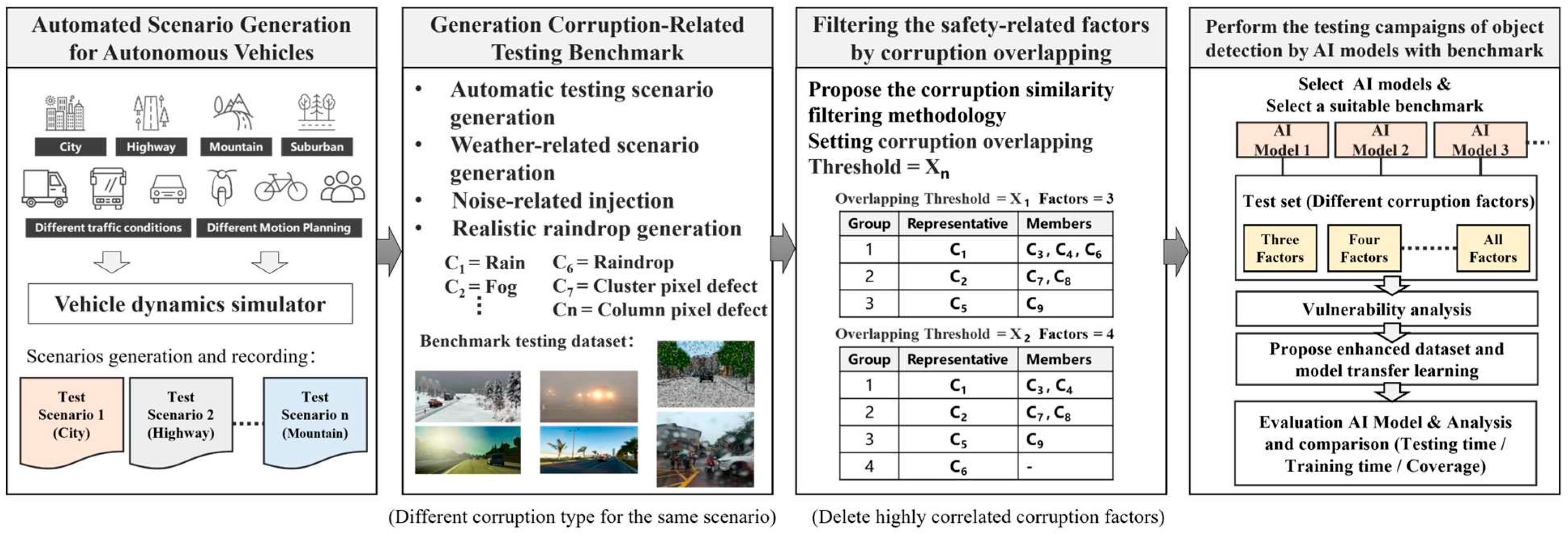
Figure 2.
An overview of the automated testing scenario generation process using VTD.
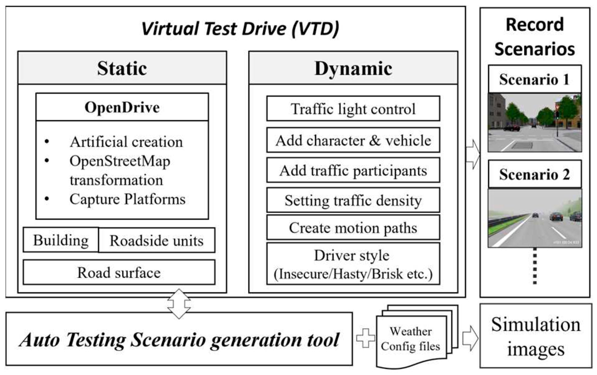
Figure 3.
Workflow diagram of the automated testing scenario generation tool.
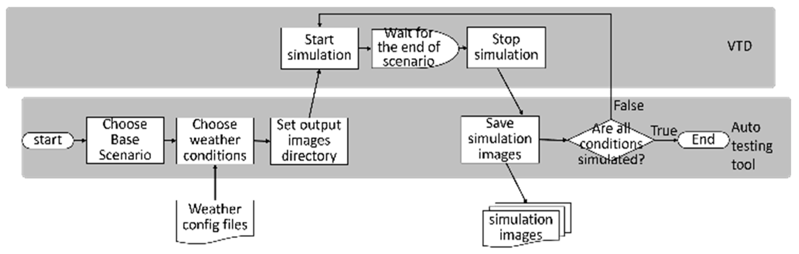
Figure 4.
VTD environmental simulation of different weather conditions. (a) no rain; (b) rain; (c) rain with visibility influence.
Figure 4.
VTD environmental simulation of different weather conditions. (a) no rain; (b) rain; (c) rain with visibility influence.
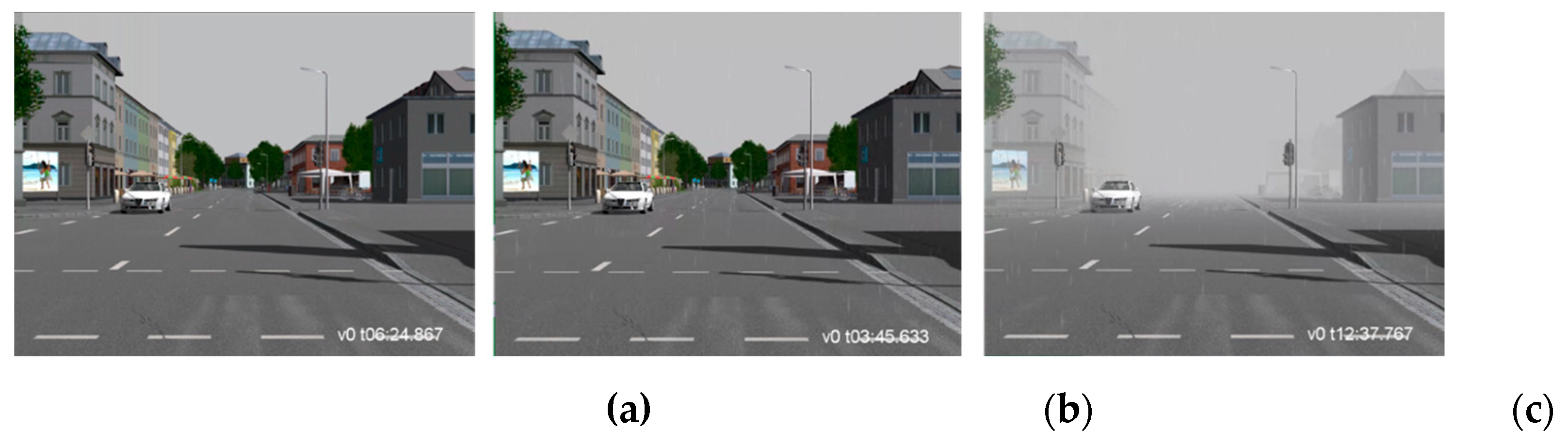
Figure 5.
Workflow for generating noise-related and raindrop images.
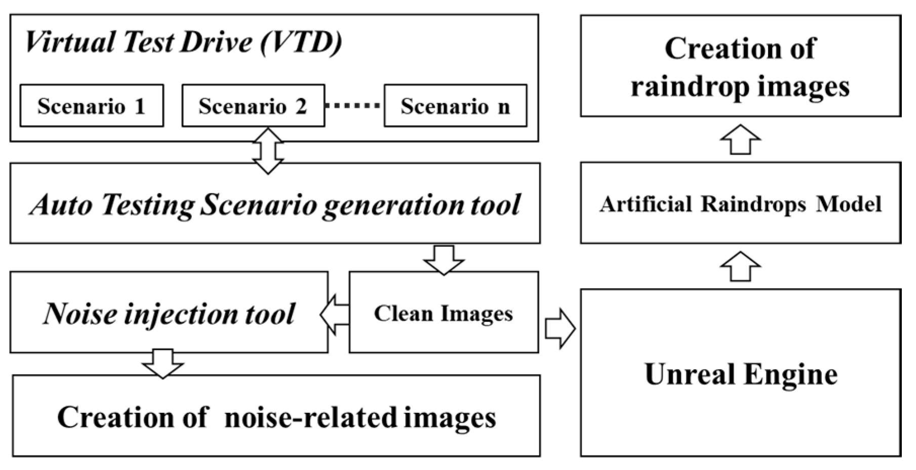
Figure 6.
Comparative analysis of the impact of noise corruption on object detection models in images (a) no corruption (b) noise corruption.
Figure 6.
Comparative analysis of the impact of noise corruption on object detection models in images (a) no corruption (b) noise corruption.
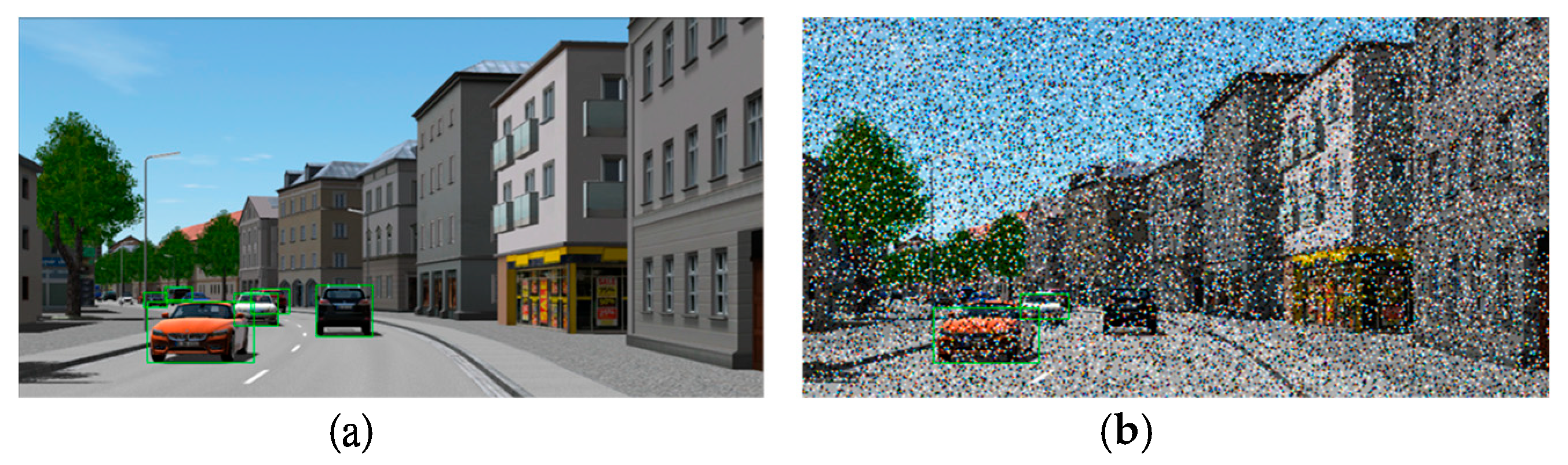
Figure 7.
Corruption percentage for different severity levels of noise corruption types.
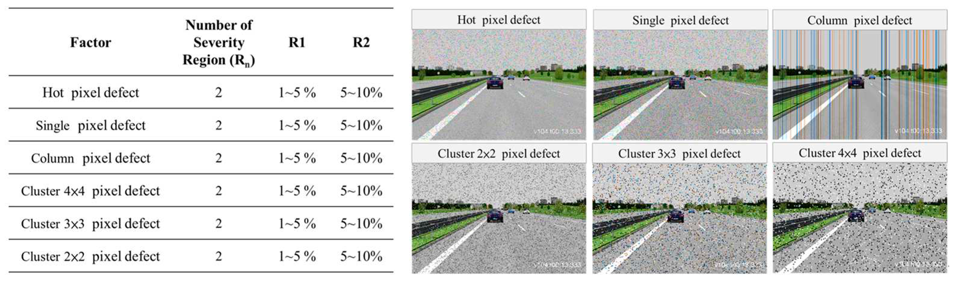
Figure 8.
Comparison between real raindrops [36] and simulated raindrop models.
Figure 8.
Comparison between real raindrops [36] and simulated raindrop models.
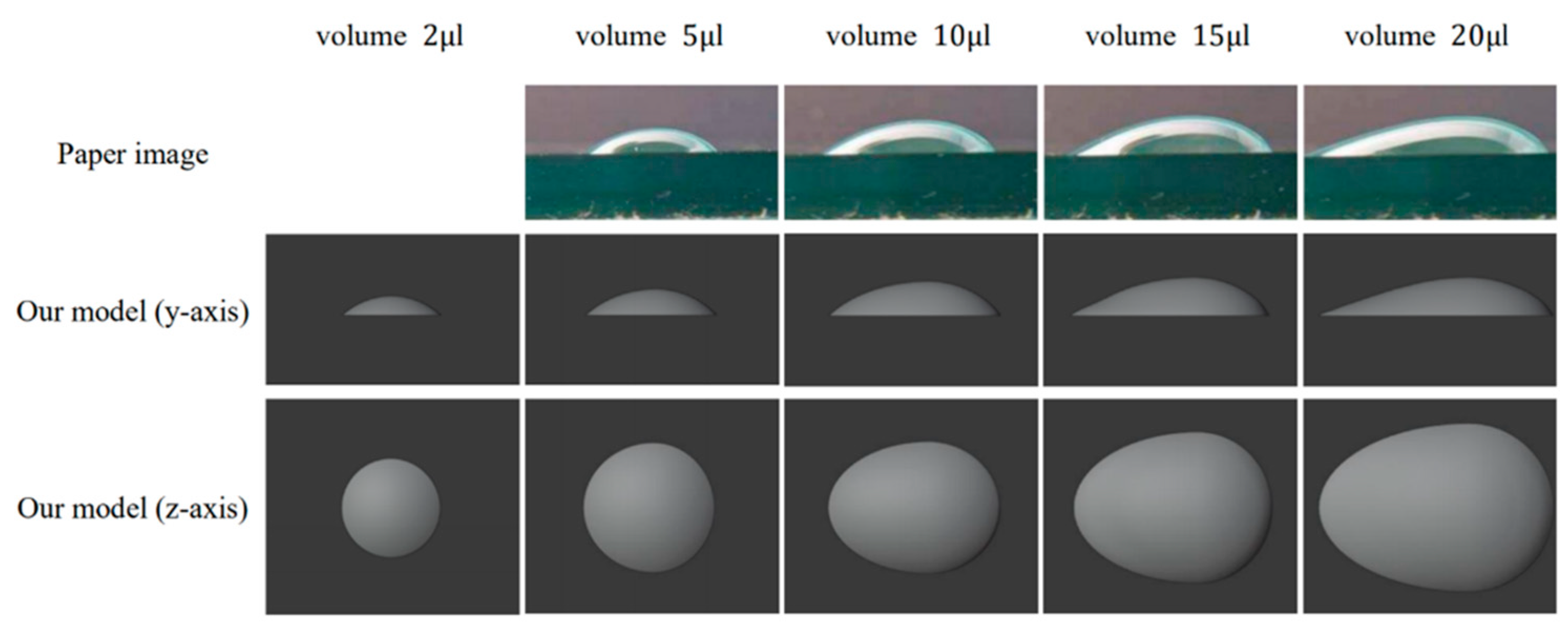
Figure 9.
Overlapping analysis procedure and corruption filtering concept among different corruption types. (a) generation of scenario corruption; (b) training and benchmark testing datasets; (c) corruption overlap score table; (d) results of corruption filtering methodology and benchmark types.
Figure 9.
Overlapping analysis procedure and corruption filtering concept among different corruption types. (a) generation of scenario corruption; (b) training and benchmark testing datasets; (c) corruption overlap score table; (d) results of corruption filtering methodology and benchmark types.
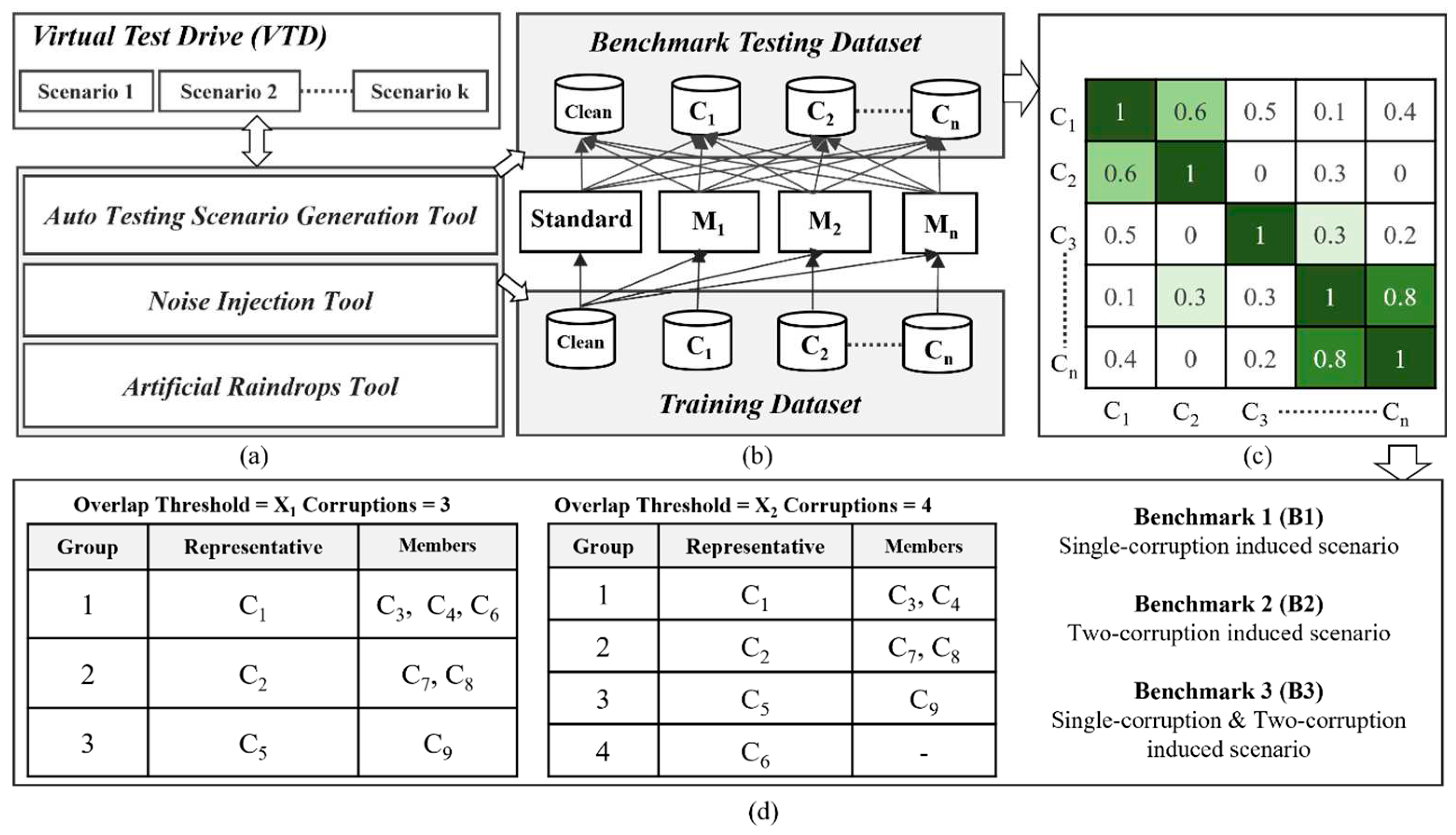
Figure 10.
Comparison of corruption effects in different severity regions for nine corruption types.
Figure 10.
Comparison of corruption effects in different severity regions for nine corruption types.
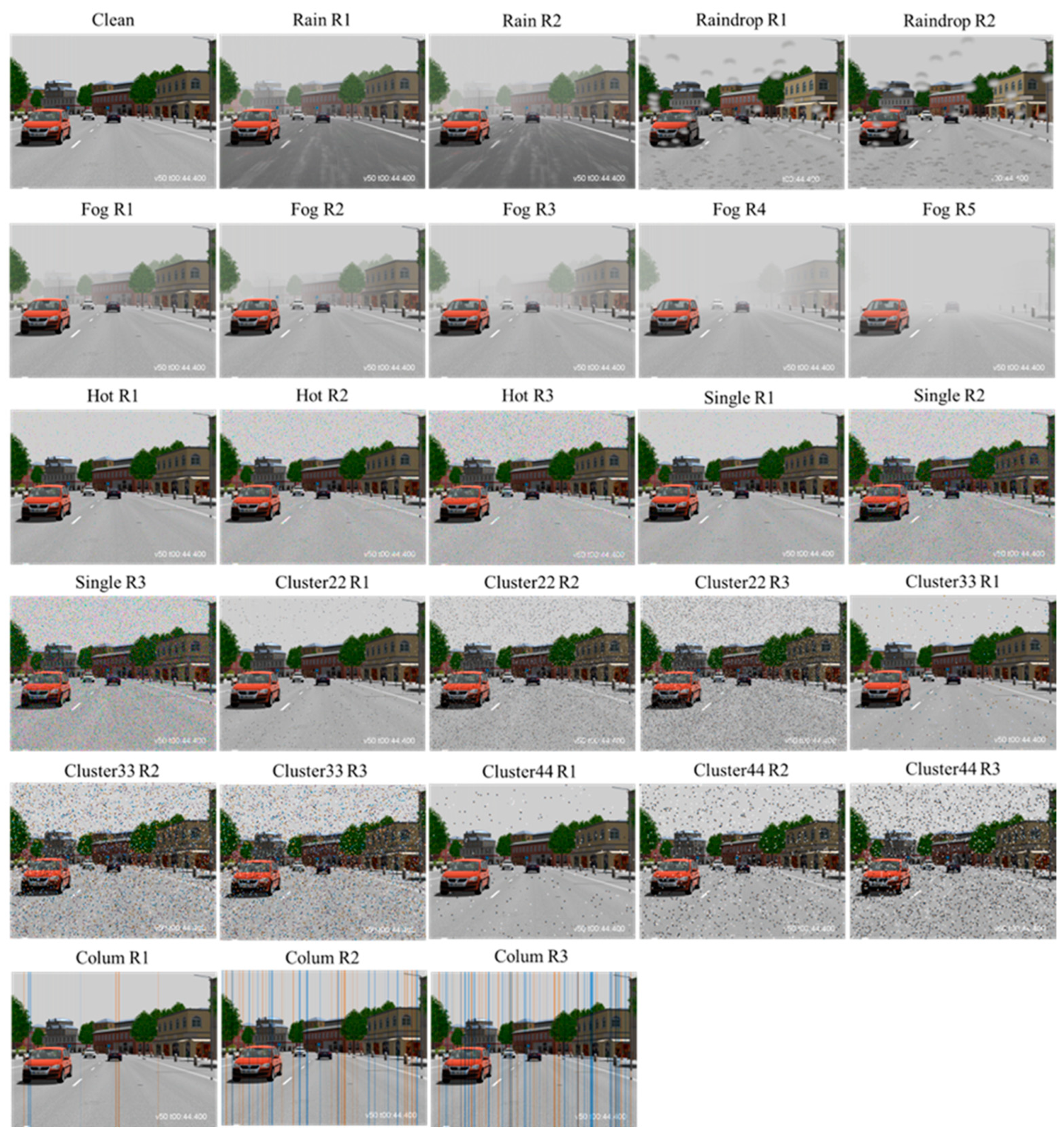
Figure 11.
Overlapping score matrix for corruption types in city and highway scenarios. (a) city; (b) highway.
Figure 11.
Overlapping score matrix for corruption types in city and highway scenarios. (a) city; (b) highway.
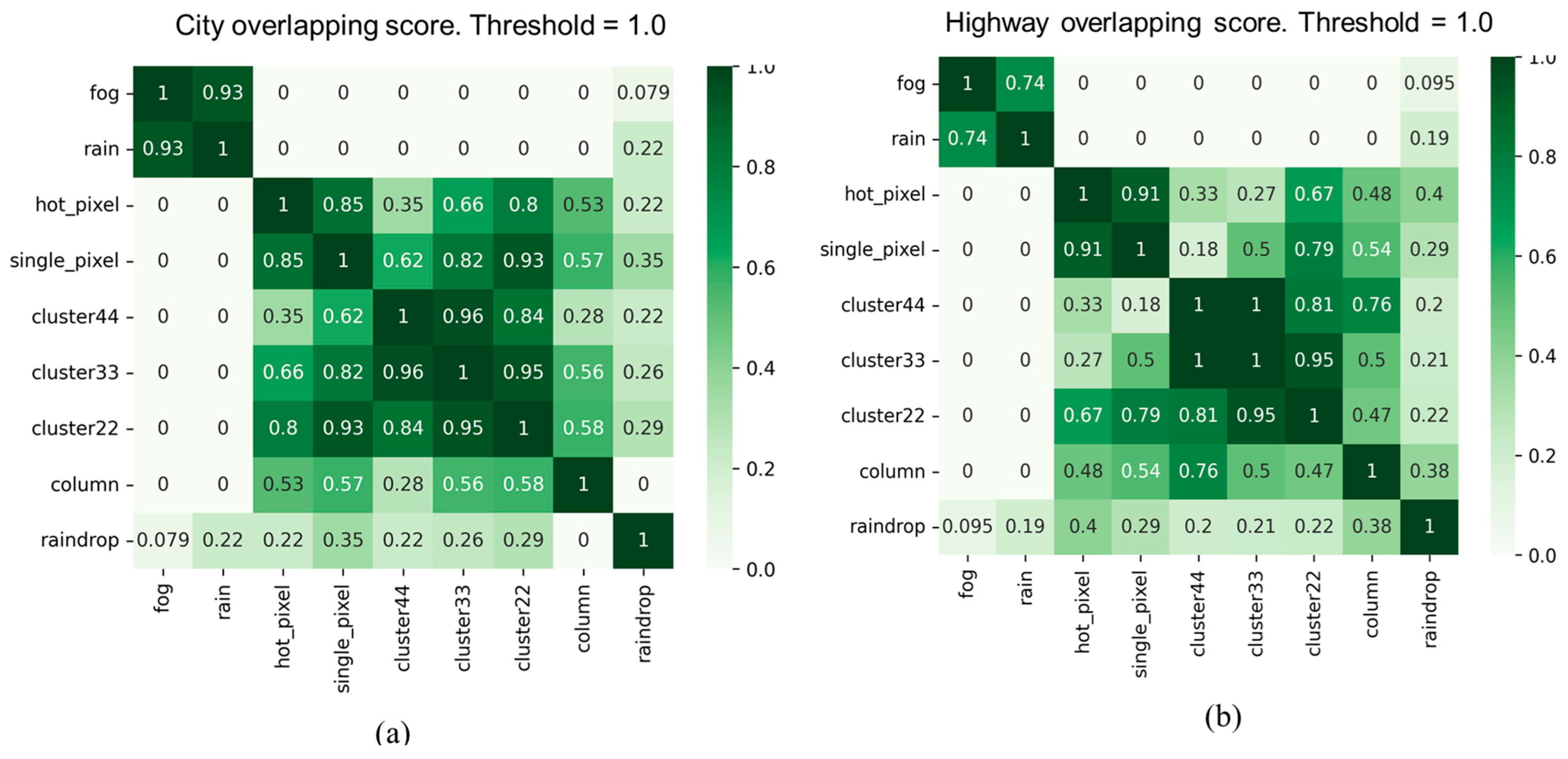
Figure 12.
Filtered corruption types in city scenario with different thresholds. (a) threshold =0.4; (b) threshold = 0.6.
Figure 12.
Filtered corruption types in city scenario with different thresholds. (a) threshold =0.4; (b) threshold = 0.6.
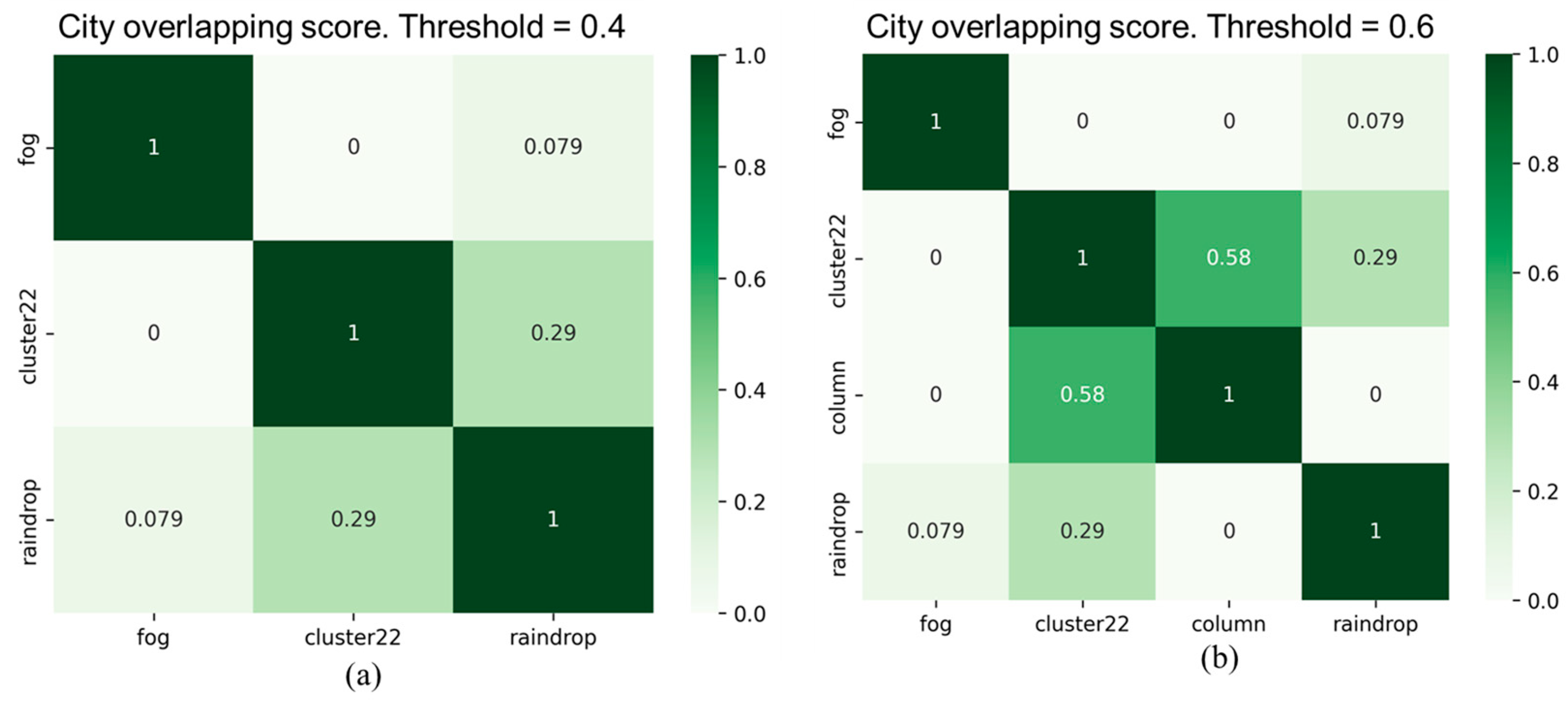
Figure 13.
Filtered corruption types in highway scenario with different thresholds. (a) threshold = 0.4 (b) threshold = 0.5.
Figure 13.
Filtered corruption types in highway scenario with different thresholds. (a) threshold = 0.4 (b) threshold = 0.5.
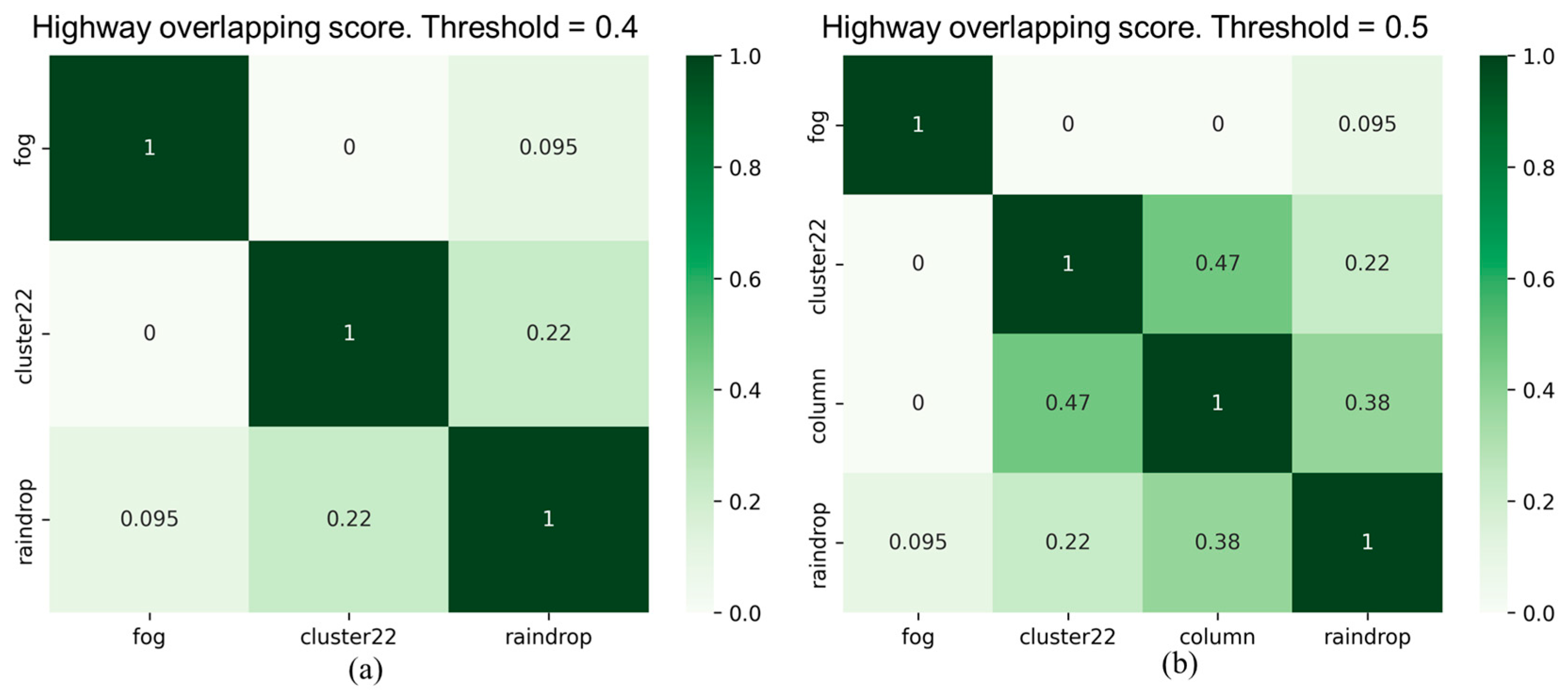
Figure 14.
Corruption groups formed by different thresholds in city and highway scenarios.
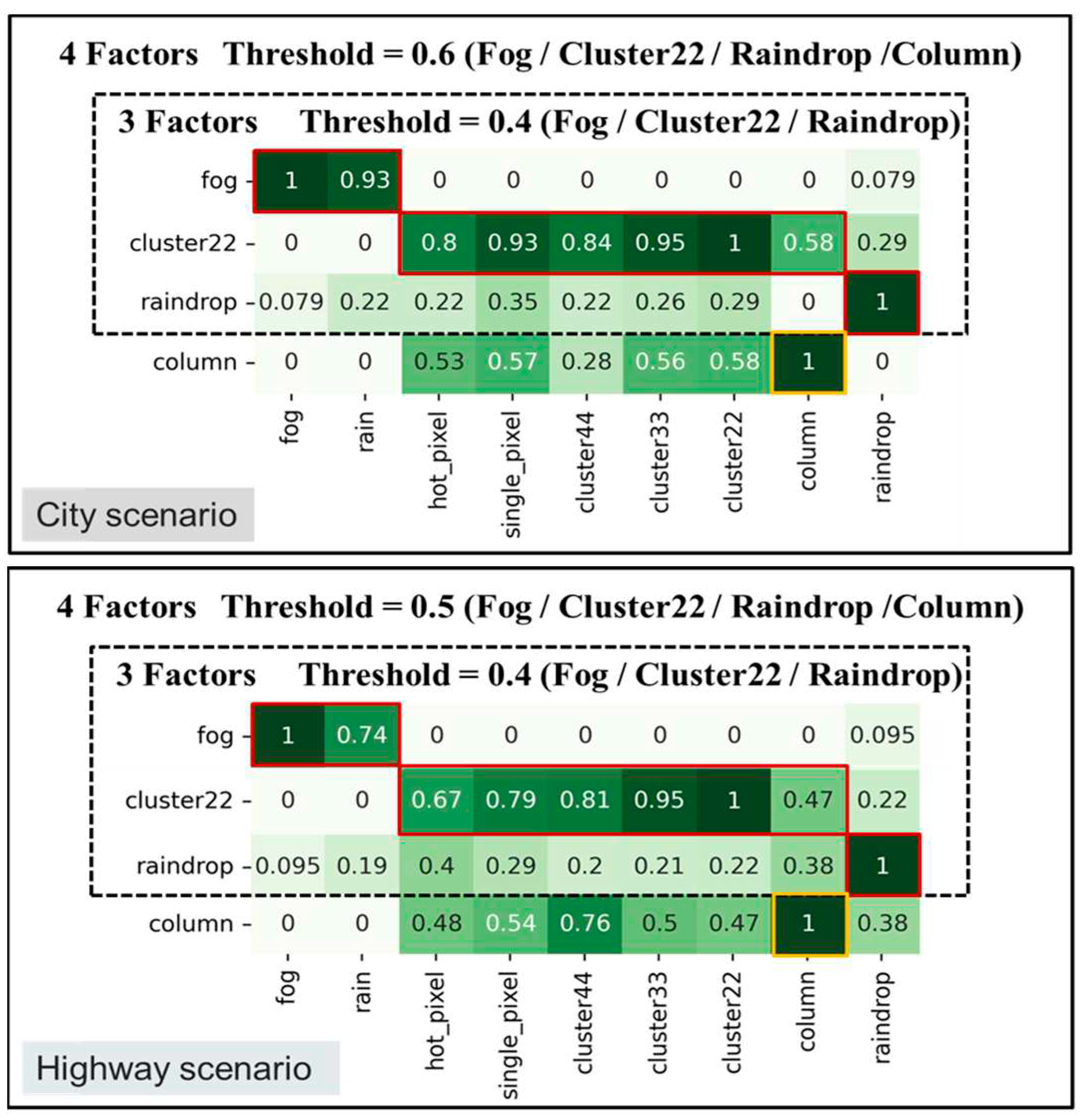

Table 1.
Definition of severity regions for various weather-related corruption types.
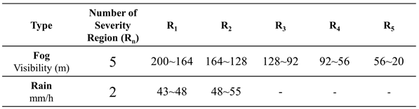 |
Table 2.
Subinterval definitions for severity regions of different weather-related corruption types.
Table 2.
Subinterval definitions for severity regions of different weather-related corruption types.
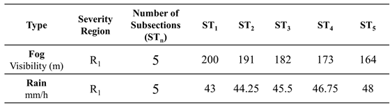 |
Table 3.
Weather parameters.
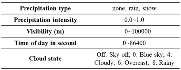 |
Table 4.
Severity levels of hourly rainfall and their corresponding visibility.
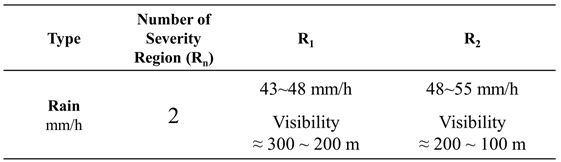 |
Table 5.
Raindrop models and their corresponding raindrop volume size ranges.
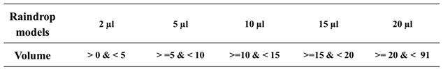 |
Table 6.
Comparative analysis of models trained on different datasets and tested on various testing sets.
Table 6.
Comparative analysis of models trained on different datasets and tested on various testing sets.
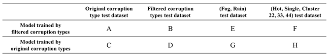 |
Table 7.
Severity setting for subregions of the worst-performing region in single corruption type detection.
Table 7.
Severity setting for subregions of the worst-performing region in single corruption type detection.
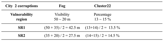 |
Table 8.
Detection performance of different trained models on single and two corruption type combinations benchmark testing datasets.
Table 8.
Detection performance of different trained models on single and two corruption type combinations benchmark testing datasets.
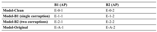 |
Table 9.
Number of severity regions and descriptions of severity levels for corruption types.
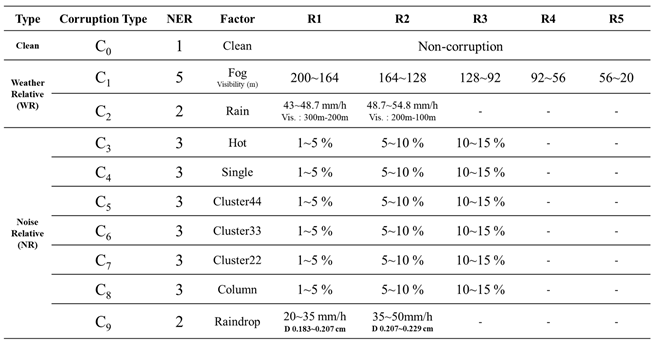 |
Table 10.
Test datasets generated for corruption types at different severity levels.
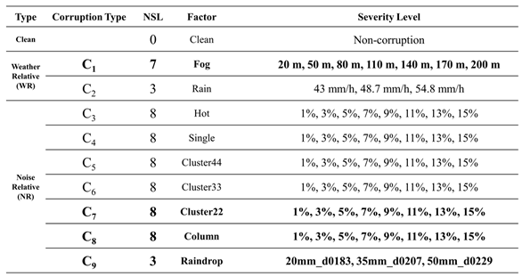 |
Table 11.
Test results for city and highway scenes.
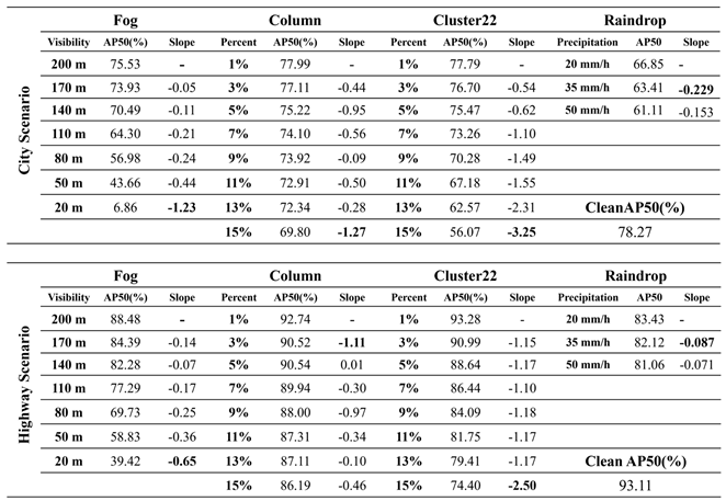 |
Table 12.
Number of images and training time required for model reinforcement training on city and highway scenarios.
Table 12.
Number of images and training time required for model reinforcement training on city and highway scenarios.
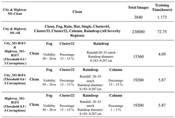 |
Table 13.
Performance of three representative corruption type training models on various test datasets. (a) city model and scenario; (b) highway model and scenario.
Table 13.
Performance of three representative corruption type training models on various test datasets. (a) city model and scenario; (b) highway model and scenario.
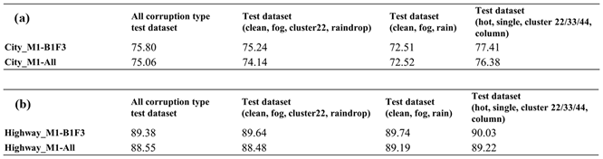 |
Table 14.
Performance of four representative corruption type training models on various test datasets. (a) city model and scenario; (b) highway model and scenario.
Table 14.
Performance of four representative corruption type training models on various test datasets. (a) city model and scenario; (b) highway model and scenario.
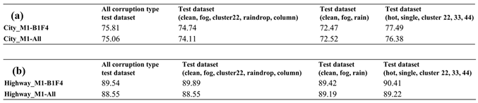 |
Table 15.
Examples of two corruption type combinations.
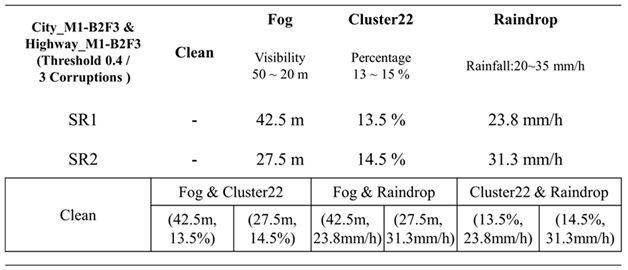 |
Table 16.
Performance of single and two-corruption type trained models in city and highway scenarios on single and two-corruption test datasets. (a) city environment; (b) highway environment.
Table 16.
Performance of single and two-corruption type trained models in city and highway scenarios on single and two-corruption test datasets. (a) city environment; (b) highway environment.
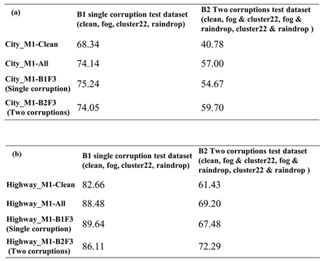 |
Table 17.
Performance of models trained by simulation scenarios tested on real-world adverse test datasets. (a) city model; (b) highway model.
Table 17.
Performance of models trained by simulation scenarios tested on real-world adverse test datasets. (a) city model; (b) highway model.
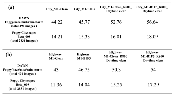 |
Disclaimer/Publisher’s Note: The statements, opinions and data contained in all publications are solely those of the individual author(s) and contributor(s) and not of MDPI and/or the editor(s). MDPI and/or the editor(s) disclaim responsibility for any injury to people or property resulting from any ideas, methods, instructions or products referred to in the content. |
© 2023 by the authors. Licensee MDPI, Basel, Switzerland. This article is an open access article distributed under the terms and conditions of the Creative Commons Attribution (CC BY) license (http://creativecommons.org/licenses/by/4.0/).
Copyright: This open access article is published under a Creative Commons CC BY 4.0 license, which permit the free download, distribution, and reuse, provided that the author and preprint are cited in any reuse.


