
Submitted:
16 November 2023
Posted:
17 November 2023
You are already at the latest version
Abstract
In the research we consider a structure-fluid interaction of oscillating piezodevice and acoustic liquid. Such problem requires finding resonance or anti-resonance frequencies of the solid structure to use them in the latter frequency-response analyses step. After finite element discretization of the issue, we need to solve a generalized eigenvalue problem (GEP). The most efficient numerical method for solving the partial GEP is the shift-and-invert Lanczos method. Each step of this algorithm requires solving a large scale system of linear algebraic equations (SLAEs) with special properties. Various ways of ordering grid nodes lead to coefficient matrices with different structure. Several methods are compared in terms of efficiency. The results of the numerical experiments are presented.
Keywords:
Numerical methods
; partial generalized eigenvalue problem
; Lanczos algorithm
; acoustic liquid
; fluid-structure interaction
1. Introduction
The problem of finding eigenvalues and eigenvectors of matrices is one of the main problems in computational physics and mathematics. One has to face this issue in the study of natural vibrations of various mechanical systems, vibrational and electronic spectra of molecules and crystals. This problem is of fundamental importance for quantum mechanics, which has become the basic discipline for studying the microcosm.
According to one of the main provisions of quantum mechanics, all observable quantities are eigenvalues of certain infinite-dimensional Hermitian operators. In addition, the finite element approximation of mathematical physics problems leads to the solution of this objective. At present, an important feature of these problems is the huge order of their matrices - up to a million or more unknown ones. Due to high orders, despite the sparse structure of matrices, the solution of such problems requires significant computing resources.
When creating preconditioners in the mixed finite-element approximations of the Stokes problem, structural mechanics and coupled problems, in the regularized interior-point methods, in the hydrodynamics, both in the theory and the constructing of the SLAE solvers, a difficult problem has to be solved. This is a generalized eigenvalue problem (GEP).
Finding eigenvalues of large scale sparse matrices is a rapidly developing area of numerical analysis, since solution of this problem became possible only with the advent of modern parallel computers. Previously, these problems were solved for small and moderate size matrices, and mainly using direct methods. At the moment, the most popular methods for solving the partial eigenvalue problem are the Krylov subspace methods [1,2,3]. The main operation of these algorithms is matrix-vector multiplication, i.e., an operation that effectively uses the possibilities of parallel computing.
In this study we consider a model of an electro-elastic body in the acoustic liquid:
Acoustic liquid can be described as:
where is stress tensor, is an eigenvalue, j is density for both solids and liquids, is deformation, u is displacement, D is electrical induction, E is electric field, are mass forces, is electrical potential, , , are damping coefficient, , , are stiffness, piezomodules and dielectric permittivity, correspondingly, index j is a body number for multybody problems. For acoustic liquid part: c is speed of sound, s is speed vector, is a vector of speed potentials, p is sound pressure, I is unit tensor, b is dissipation coefficient.
This model describes piezoelectric materials that can be used as energy transformers and harvesters, as part of medical equipment, in non-damaging control and other applications. To find natural frequencies and corresponding shapes we need to solve the GEP for the model (1)-(6). These frequencies are useful in solving frequency-response fluid-structure problem for forced oscillations of the piezobody and some liquid that includes equations (7)-(10).
In this research we focus on the discretization of (1)-(6) as described in [4] to obtain the following GEP:
where is an eigenvalue, v is an eigenvector. The stiffness matrix is symmetric quasi-definite (SQD) [5,6,7,8], and the mass matrix is symmetric positive semidefinite. In (11) neither nor is positive definite, but real scalars a and b are exactly known such that is positive definite (e.g., ) and we have a symmetric definite pencil [2,3]. Then, the simultaneous diagonalization of two matrices of the pencil by a congruent transformation is possible [2]. Note that the eigenvalues sensitivity depends on the condition number of the diagonalizing matrix. Both matrices in (11) are large and sparse and the structure of and is following:
where , and are symmetric positive definite matrices (SPD). The properties of the SQD matrices established in [5,6,8], namely, SQD-matrix is square, symmetric, indefinite, nonsingular, and the inverse matrix is also SQD. In Figure 1 the structure of the stiffness and the mass matrices is shown.
The SLAEs with SQD-matrices also appear in the mixed finite-element approximation to the globally stabilized Stokes problem in weak form. After discretization with triangular elements and continuous linear pressure, we obtain the SQD-system, where E is the gradient matrix, is the divergence matrix, P is the vector-Laplacian matrix and R represents the stabilization term [8,9]. If then a saddle point linear system appears which is solved in hydrodynamic problems of a viscous incompressible fluid, in particular, when solving the Navier-Stokes equations [10,11,12]. "Discretization of the Oseen problem using, e.g., finite differences or finite elements results in a generalized saddle point system. Algorithms for solving both standard and generalized eigenvalue problems for saddle point matrices have been studied in the literature, particularly for investigating the stability of incompressible flows and in electromagnetism" [10] and references there.
The purpose of the research is to evaluate the performance of the Shift-and-Invert (SI) Lanczos method [1,3,13,14,15] for the GEP (11) with different ways of the SLAE solving. All eigenvalues of (11) are real and positive but some of them are infinite [1,3]. In [1] it is shown that the Lanczos algorithm can be run directly on the pencil if and certain SLAEs with can be solved. To improve the convergence rate we should use a spectral transformation [3,14,15].
Denote the rank of and then the spectrum of (11) has r finite eigenvalues , the remaining eigenvalues being at infinity . The eigenvectors related with the eigenvalues at infinity are such that . The eigenvectors corresponding to the finite eigenvalues can be -orthonormalized, i.e., , where is the Kronecker delta.
Circumscribing of the SI Lanczos algorithm can be found in [3,14,15]. Let is choose a scalar , not equal to any eigenvalue, and we seek a few eigenvalues closest to . Then (11) is changed into
where is identity matrix, .
Let Lanczos algorithm with an initial vector b constructs a matrix whose columns form the -orthonormal basis for the Krylov subspace [1]. For there is a three-term recurrence [3]
where , , and , when is such that . We can rewrite (13) as
where is the mth unit vector, and is tridiagonal matrix with along the diagonal, and along the subdiagonal and superdiagonal. The orthogonal projection of the eigenvalue problem on the range of gives the solution with , and the residual is [2,3,15].
The matrix in (13) is not calculated. Instead, the SLAE with is solved each time a matrix needs to be multiplied by a vector. To compute the eigenvectors it is necessary to store all calculated Lanczos vectors. This requires a large amount of memory and it cannot be determined in advance, since the number of iterations is unknown. To solve this problem, restarting version of the Lanczos method is used [3]. Moreover, when solving a problem with a singular mass matrix, it is necessary to choose the initial vector in a special way. The Lanczos and the Ritz vectors have components in the nullspace of the mass matrix and its magnitude can increase during iterations. To solve this problem the starting vector must be placed in the proper subspace [15].
Let and be the minimum and the maximum of the finite eigenvalues of (11), and
When then the matrix is SQD, if then this matrix is indefinite because the positive definiteness of the (1,1) block is lost. When it has only one positive eigenvalue, the rest are negative, and when the matrix becomes negative definite. A matrix type knowledge is fundamental when choosing a SLAE solver. Since in practice the lower part of the GEP spectrum is of interest (usually several smallest eigenvalues), we assume that it is necessary to solve a SLAE with SQD (e.g., with ) or indefinite matrices. Figure 2 shows spectrum of the matrix depending on the value.
Often in the literature [2,16] etc., a direct method for solving SLAE is used based on matrix factorization. It is known [5,16] that SQD-matrix is strictly factorizable, i.e., for any permutation matrix , there exists a lower triangular matrix L (with unit diagonal) and a diagonal matrix D (generally indefinite) such that . In [16] stability results for factorization of SQD matrices have been provided. But when using the Cholesky decomposition, the main problem is the absence of an ordered structure of the matrices in the presence of strong sparseness, i.e., the predominant number of the zero elements. Moreover, our computations showed that factor L becomes completely fill-in and for large problems such factorization is too expensive or completely impossible.
An another approach is the iterative SLAE solving. These systems do not necessarily need to be solved very accurately. There are some strategies for choosing accuracy for SLAE solving, e.g., [17]. Sometimes, as the number of SI Lanczos iterations increases, these systems can be solved less accurately. On the other side, outer iterations can slow down if inner steps are not enough. Since is SQD or indefinite matrix, several approaches can be used to solve the SLAE with it.
- Transition from SLAE with SQD matrix to the equation system with a block non-symmetric positive definite matrix
- Reducing the SLAE dimension using Schur’s complement and/or preconditioning of the inner iterative solver
- Solving the SLAE with block-banded matrix that has an ordered structure and obtained by different nodes numbering
Let us consider each of these approaches.
We implement the methods and consider its robustness. The computations for the model matrix pencil are performed with MATLAB (R2019a). Because we do not know the exact solution of (11), at first, we compared the computed Ritz values with the eigenvalues obtained by MATLAB’s built-in solver EIGS.m for the sparse GEP. For the non-zero matrix block in (12) we have , i.e., the model pencil has 375 positive real finite eigenvalues. To control convergence in the SI Lanczos algorithm, we check for the residual norm which is cheaply computed [2,3]. We use full reorthogonalization of the Lanczos vectors to obtain the best eigenvalues accuracy. In practice, the residuals become small without this procedure, but the accuracy of the computations will be worse. QR-algorithm is used to calculate the Ritz values of the tridiagonal matrix.
2. SLAEs with a positive definite matrix
PROPERTY [5,6]. "Let . Then, for any SQD matrix , the matrix
is non-symmetric positive definite; i.e., its symmetric part
is positive definite. Note that a non-symmetric matrix with a positive definite symmetric part has its field of values contained in the right half-plane [6,10]; in particular, all eigenvalues of have positive real parts. If z is the SLAE solution with coefficient matrix , and w is the corresponding solution with coefficient matrix , then ". An analogous result holds for indefinite matrices [10].
A lot of methods exist for solving such SLAEs, we will mention some of them: HSS [20], IHSS [21], their modifications and generalizations [22,23], GSOR [24], Multigrid Methods (MGMs) [25,26], PSTS [27] and others.
In Table 1 we give the nine smallest magnitude eigenvalues computed by the SI Lanczos algorithm with the PSTS (Product-Type Skew-Hermitian Triangular Splitting) solver (one of the authors participated in its development). Here is the MATLAB-solution, is the computed Ritz values and is the modulo differences. We also can apply MGM using PSTS as a smoothing procedure [28]. Since the number of the multigrid iterations is comparable to the number of PSTS iterations, we give computations with the latest SLAE solver. Moreover, PSTS iterative method can be used as a preconditioner when solving SLAE with the coefficient matrix (14) [27].
3. Schur complement reduction
Let us rewrite GEP (11) in the block form
where Let
is the Schur complement of the block R in the matrix (denoted ), then we obtain the smaller size GEP
containing only SPD matrices and . The matrix S is SPD by virtue of Sylvester’s law of inertia [1] and
One of the most costly operations in the formation of the Schur complement is the inversion of R. Usually, methods for finding the inverse matrix are poorly parallelizable direct methods, e.g., the inversion method based on -decomposition. In the mesh issues arising from discretizations of boundary value problems in mathematical physics usually looking for efficient approximations for S since the computation of the exact one is too time-consuming.
Since the both matrices in (16) are SPD ones, the Lanczos method without shift and inversion can be used. It finds the eigenvalues of the symmetric GEP (16) by a Rayleigh-Ritz procedure [1,2,3]
The action of S on the column vectors y can be computed by means of matrix-vector products with matrices , E, P and by solving a linear system with matrix R [10]
To control the robustness of the Lanczos method without spectral transformation, we check the coincidence of the Ritz values with the eigenvalues along the entire spectrum in Figure 4.
Nevertheless, the SI Lanczos method with the inner preconditioned solver can also be used. The Schur-complement equation is
Since we are interested in several smallest eigenvalues closest to zero, we can put . Then (18) takes a more simple form
We have to apply a method which requires only matrix-vector multiplications by S in addition to inner products and operations like "saxpy" (adding a multiple of one vector to another), e.g., the Conjugate Gradient Method (CGM) [1,2,29].
In [8] it was noted that
where is SPD matrix, and In (15) P and R are easily invertible (i.e., the SLAE with these matrices can be easily solved). The convergence rate of the CGM is usually improved by a suitable preconditioner.
RESULT [8] "The generalized CRAIG [30] method iterates are related to the iterates of the CGM applied to equation with preconditioner P, according to "
The Craig’s method is actually a reorganized CGM applied to the normal equations (CGNE [29]). Denote Then we can rewrite (19) as
It is obvious that (20) is the preconditioned SLAE
where , and . The matrix P is the preconditioner which is introduced implicitly. The matrices and are similar, therefore they have the same spectrums.
RESULT [7] "The extended CRAIG iterates are related to the CGM iterates for the problem according to "
Here is an auxiliary variables, is the regularization parameter equal to one in (20). The Preconditioned CGNE (PCGNE) method was given in [29]. At each step of this algorithm, it is necessary to solve the SLAE with matrix P to find the current value of the residual and compute the matrix-vector product with matrix S. We take termination criterion for the Schur-complement equation (19) as , where is the residual at k-iteration. An alternative approach is to limit iterative method to a fixed number of inner steps, but this may negatively affect the convergence rate of the outer iterations. Numerical results for the smallest closest to zero, the corresponding Ritz value and the modulo differences for the moderate-dimension matrices are given in Table 2. Here n is the block-structured matrices dimension in (15) and "IT" is a number of PCGNE iterations.
As the size of the matrices increases, the number of inner PCGNE iterations also increases and the accuracy of the computed Ritz values deteriorates somewhat. It turns out to be worse than the previously obtained accuracy by the iterative PSTS method. This is a consequence of using the method for the normal equations. Note that in [31] preconditioned Lanczos algorithm had an eigenvalue problem in the inner loop instead of a linear equations problem. The SI Lanczos method with the inner preconditioned CG iterations was taken for comparison of the numerical results in this research.
4. The SLAE with block-banded matrices
We can order the unknowns (namely, grid nodes) in the GEP (11) in different ways and get different structured matrices. Several variants of such structures are shown in the figures below. In Figure 5 we show the stiffness and mass matrices, which have a similar structure, but differ in their properties and the number of non-zero elements.
For such structured matrices ILU (Incomplete LU factorization), iterative ILU or MILU (Modified ILU) [16,32] can be used. A large number of methods are developed for the special issues, whereas parallel ILU (MILU) are more general. We can use these methods both as SLAE solvers and preconditioners.
In Table 3 we give the computed data using the Crout ILU method [32] in comparison with LU factorization and error norm. The Crout’s algorithm in its generalized form is an LU-factorization, where L is a lower triangular matrix and U is an unitary upper triangular matrix. Note that unlike the methods mentioned above, ILU and MILU factorizations require optimal implementation of sparse matrix-vector and also matrix-matrix products.
In Table 4 we give nine eigenvalues closest to zero computed by the SI Lanczos algorithm with the Crout ILU for the matrix pencil, . As expected, the use of the direct method gives a higher accuracy of the sought Ritz values than all iterative methods, even the latter are preconditioned. Therefore, parallel implementations of direct solvers are promising, provided that they can store vectors of the required size.
5. Program implementation in ACELAN-COMPOS package
For the purpose of demonstrating the implemented modules, we show a test model of piezodevice. Let us consider a model of piezo-active transducer shown in Figure 6 that is working in the acoustic liquid.
The transducer is 10 cm long, 2 cm wide and 2 mm thick. Short sides are fixed. Such device can be used for emitting waves in the liquid in actuator mode or as a sensor, producing energy from periodical mechanical load. Oscillations will be forced by the difference of potentials on electrodes placed on the top and on the bottom parts of the device.
For the purpose of measuring the performance of the developed algorithms, we will proceed with a 3D model of the device, even it is possible to solve presented problem in the plane form. Initial geometry, meshing and reference studies for a presented model were performed in COMSOL Multiphysics package [35] .
We implemented computational modules for described as part of ACELAN-COMPOS package [4]. This software is used for general finite element computations, but focuses on modeling composite materials with coupled fields. The package is based on a class library written in C# language. The process of solving the Eigenvalue problem consists of three main stages: assembling sparse matrices, performing operations with assembled matrices and post-processing results to obtain final values.
The first stage takes an input as combination of geometry as a mesh, problems statement that includes an element implementation, materials and boundary condition. For each volume in a mesh corresponding local matrix should be computed. If two elements have the same geometry and material properties and the only difference between them is a position in the geometry, their local matrices are identical. The mesh that consists of such element is called a regular mesh. In this case, the caching and re-using of once computed local matrices can reduce the computational time. If the shape of analyzed body allows to build a quad mesh and sweep for the whole body, the quasi regular mesh can be used in the same manner. For majority of shapes tetrahedral meshes are used, and this technique is not possible, and for this case the simple parallelization can be used to build local matrices effectively. The next step is to transfer value from local matrix to global. Since the finite element method produces sparse matrices, the underlying data structure becomes the bottleneck for matrix operations. It is crucial for Lanczos method implementation to have fast and reliable matrix-vector multiplication operation. Some sparse data formats are more effective for reading and setting values by coordinates, other are optimized for multiplication [33]. ACELAN-COMPOS package supports multiple formats, and usually the assembling and further matrix operations are performed with two different data structures: assembling process is faster for hash-table based structures, and further computing is more effective for compressed rows or columns formats.
The structure of a geometry mesh is important for the output matrix. Each column and row represents a single nodal degree of freedom. If the three dimensional mechanical problem is considered, each node with be represented as 3 rows and columns, these rows usually numbered sequentially, for node with index i these rows will be numbered . Lets consider a different node with index j. If there is an element that includes nodes i and j, in row values at columns will be filled. Some formats, like SKS (Skyline Storage), based on filling the whole section of the matrix row from the first non-zero value to the last. For that reason the indexing of nodes is important for both the size of data structure and the speed of computation. There are multiple methods for compressing the structure by re-enumerating nodes, but for quasi regular mesh trivial coordinate sorting allows to achieve the most effective structure. Another option to be considered is the sorting of degrees of freedom in the node. If piezomaterial is considered, mechanical and electrical unknowns can be grouped on node level or on the whole global matrix level.
The second stage is based on the matrix-vector and matrix-matrix multiplication. ACELAN-COMPOS package can be executed on different platforms and hardware. The client version of the package is intended to be used on consumer grade computers and laptops. For such devices limited amount of RAM should be considered, but multi-core processors (Intel Core and AMD Ryzen) series allow to perform basic parallelization. The server version usually runs on hardware with extended amount of RAM and multi-core server processors (Intel Xeon series). Such setups perform worse that consumers hardware in single-core scenarios, but since amount of memory allows to solve multiple problems simultaneously, multi-level of parallelization can be utilized. In this paper we also consider an effective processors (AMD Threadripper Series) with high single core speeds and multiple thread possibilities. We compared basic computational operations for sparse matrices on all three described setups, with underlying structures and methods implemented in CSPARSE [34] with bindings for un-managed code and native C# implementation.
For a model presented in Figure 6 rough or fine mesh can be suggested. Since measurements of the device are significantly different, we performed numerical experiments with three meshes: two regular with cubic elements (named A and B) and optimized mesh of hexagons (named C) as shown in Figure 7. The difference in obtained eigenvalues between meshes was below 2%.
Computations were performed for two basic operations: assembling of global matrices, including loading mesh into memory and all needed operations with data formats, and matrix-vector multiplication for a sparse stiffness matrix (Figure 8) and random vector. Matrix-vector multiplication was performed on single core. Meshes were imported into the ACELAN-COMPOS package as .nas files. Boundary conditions were re-applied. Numerical results obtained on generic consumer laptop (AMD Ryzen 7 4800H CPU, 32 Gb RAM) are presented in Table 5.
Computations were also performed on different workstations. Without parallelization, professional PCs (AMD Threadripper PRO 3995 WX) outperform consumers PC by 3-5%. Parallelization with built-in C# tools allows to speed computation up by 40-45% for consumer PC and up to 55% on professional PCs, depending on available RAM.
6. Conclusions
Various approaches to solving SLAEs are used in the inner loop of the SI Lanczos method when solving the partial symmetric GEP. The choice of the system solver is determined by the size and structure of the matrices. For all considered methods, an optimal implementation of sparse matrix-vector or/and matrix-matrix products is necessary. When using iterative solvers the accuracy of the SLAE solution has be no worse than the accuracy of the desired eigenvalues. Some iterative methods converge slowly and require preconditioning. This entails increase in the number of matrix-vector products and, possibly, an additional solution of the SLAE in the inner loop of the preconditioned solver. Preference should be given to direct methods (LDLT, ILU or MILU) if the possibility of parallel implementation allow. It is important to have a rough estimate of the arithmetic operations number which is required to solve the SLAE, since in the problems with large-scale sparse matrices one has to balance between the required accuracy and the amount of computational work. Developed software is optimized for specific combination of mesh properties and needed operations. Utilizing different sparse matrix storage formats along with straightforward parallelization and caching allows to speed up computations for presented algorithm. Specific platform related optimization for faster CPUs or multi-core environment with slower cores can be performed during runtime by applying users settings. Mesh structure optimizations are crucial for proper performance of the method, including the selection of form for the regular elements.
Funding
The research was funded by a grant of the Russian Science Foundation N 22-21-00318, https://rscf.ru/project/22-21-00318/ at Southern Federal University
References
- B.N. Parlett, The Symmetric Eigenvalue Problem, SIAM, Philadelphia, PA, 1998.
- J.W. Demmel, Applied Numerical Linear Algebra, SIAM, 1997.
- Saad Y., Numerical methods for large eigenvalue problems, SIAM, second edition, 2011.
- N.V. Kurbatova, D.K. Nadolin, A.V. Nasedkin, P.A. Oganesyan, A.N. Soloviev, Finite element approach for composite magneto-piezoelectric materials modeling in ACELAN-COMPOS package, Advanced Structured Materials, p. 69-88. 2018.
- R.J. Vanderbei, Symmetric quasidefinite matrices, SIAM J. Optim., 5(1), p. 100-113, 1995.
- George A., Ikramov Kh., Kucherov A.B., Some properties of symmetric quasi-definite matrices, SIAM J. Matrix Anal. Appl., v.21, N4, p.1318-1323, 2000.
- M.A. Saunders, Solution of sparse rectangular systems using LSQR and CRAIG // BIT, v. 35, p. 588 604, 1995. [CrossRef]
- M. Arioli, D. Orban, Iterative methods for symmetric quasi-definite linear systems Part I: Theory. Technical Report RAL-TR-2013-003, 2013.
- D. Silvester and A. Wathen. Fast iterative solution of stabilised Stokes systems part II: Using general block preconditioners // SIAM Journal on Numerical Analysis, v. 31(5), p. 1352 1367, 1994. [CrossRef]
- M. Benzi, G.H. Golub and J. Liesen, Numerical solution of saddle point problems, Acta Numerica, v.14, 2005, p. 1-137.
- G. Muratova, T. Martynova, E. Andreeva, V. Bavin, Z.-Q. Wang, Numerical solution of the Navier-Stokes equations using multigrid methods with HSS-based and STS-based smoothers // Symmetry, 12(2), 233, 2020.
- G. Muratova, T. Martynova, E. Andreeva, V. Bavin, Z.-Q. Wang, Multigrid methods with PSTS- and HSS-smoothers for solving the unsteady Navier-Stokes equations // SEMR, v.17, p.2190-2203, 2020. [CrossRef]
- Lanczos C., An iteration method for the solution of the eigenvalue problem of linear differential and integral operators, J. Res. Nat. Bur. Standards, Sect. B, v. 45, p. 255-281, 1950.
- T. Ericsson and A. Ruhe, The spectral transformation Lanczos method for the numerical solution of large sparse generalized symmetric eigenvalue problems, Math. Comp., 35, p. 1251-1268, 1980.
- K. Meerbergen, The Lanczos method with semi-definite inner product, BIT, v.41, N.5, p. 1069-1078, 2001.
- P.E. Gill, M.A. Saunders, and J.R. Shinnerl, On the stability of Cholesky factorization for symmetric quasidefinite systems, SIAM J. Matrix Anal. Appl., 17 (1996), pp. 35 46.
- Morgan R.B., Scott D.S., Preconditioning the Lanczos algorithm for sparse symmetric eigenvalue problems // SIAM J. Sci. Comput., v.14, No.3, p. 585-593, 1993.
- C.C. Paige, M.A. Saunders, Solution of sparse indefinite systems of linear equations, SIAM J. Numer. Anal., 12, p. 617-629, 1975.
- S.-C. Choi, C. C. Paige, and M. A. Saunders. MINRES-QLP: A Krylov subspace method for indefinite or singular symmetric systems. SIAM J. Sci. Comput., v. 33(4), p.1810 1836, 2011.
- Bai, Z.-Z., Golub, G.H., Ng, M.K., Hermitian and skew-Hermitian splitting methods for non-Hermitian positive definite linear systems // SIAM J. Matrix Anal. Appl. 24, p. 603-626, 2003.
- Bai, Z.-Z., Golub, G.H., Ng, M.K., On inexact Hermitian and skew-Hermitian splitting methods for non-Hermitian positive definite linear systems // Linear Algebra and its Appl., 428, p. 413-440, 2008.
- Bai, Z.-Z., Splitting iteration methods for non-Hermitian positive definite systems of linear equations // Hokkaido Math. J. 36, p. 801-814, 2007.
- Bai Z.-Z., Golub G.H., Lu L.-Z., Yin J.-F., Block triangular and skew-Hermitian splitting methods for positive definite linear systems // SIAM J. Sci. Comput. 26, p. 844-863, 2005.
- Bai Z.-Z., Parlett B.N., Wang Z.-Q. On generalized successive overrelaxation methods for augmented linear systems // Numer. Math., 2005, v. 102, p. 1 38.
- K. Stuben, Algebraic multigrid (amg): experiences and comparisons, Appl. Math. Comput., 13, 1983, p. 419-451.
- U. Trottenberg, C. Oosterlee, A. Schuller, Multigrid, Academic Press, 2001.
- Krukier L.A., Martynova T.S., Bai Z.-Z., Product-Type Skew-Hermitian Triangular Splitting Iteration Methods for Strongly Non-Hermitian Positive Definite Linear Systems // Journal of Computational and Applied Mathematics. Vol. 232, N 1, P. 3–16, 2009.
- T.S. Martynova, G.V. Muratova, I.N. Shabas, V.V. Bavin, Multigrid methods with skew-Hermitian based smoothers for the convection-diffusion problem with dominant convection // Numerical Methods and Programming, 23 (1), p. 1-14, 2022. [CrossRef]
- Y. Saad, Iterative methods for Sparse Linear Systems, SIAM, 2nd ed., 528 p.
- J.E. Craig, The N-step iteration procedures // Journal of Mathematics and Physics, 34(1), p. 64 73, 1955.
- R.B. Morgan, D.S. Scott, Preconditioning the Lanczos algorithm for sparse symmetric eigenvalue problems // SIAM J. Sci. Comput., v. 14, N. 3, p. 585-593, 1993.
- N. Li, Y. Saad, E. Chow, Crout versions of ILU for general sparse matrices, SIAM Journal on Scientific Computing, 25(2), 2003. [CrossRef]
- Kh.D. Ikramov, Matrix pencils - theory, applications, numerical methods. The results of science and technology, Math. anal., v.29, p.3-106, 1991.
- T. Davis, Direct Methods for Sparse Linear Systems, SIAM, 2006, ISBN: 0898716136, LC: QA188.D386.
- COMSOL Multiphysics v. 5.6. www.comsol.com. COMSOL AB, Stockholm, Sweden. (License 9602094).
Figure 1.
Sparsity patterns of the stiffness (left) and the mass (right) matrices
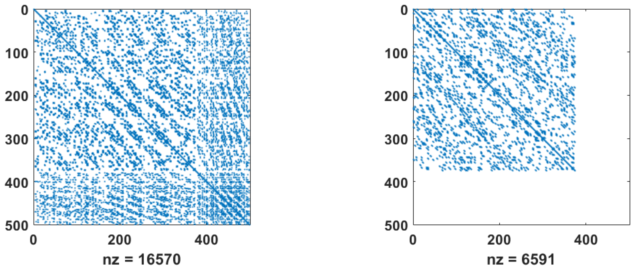
Figure 2.
Spectrum of for
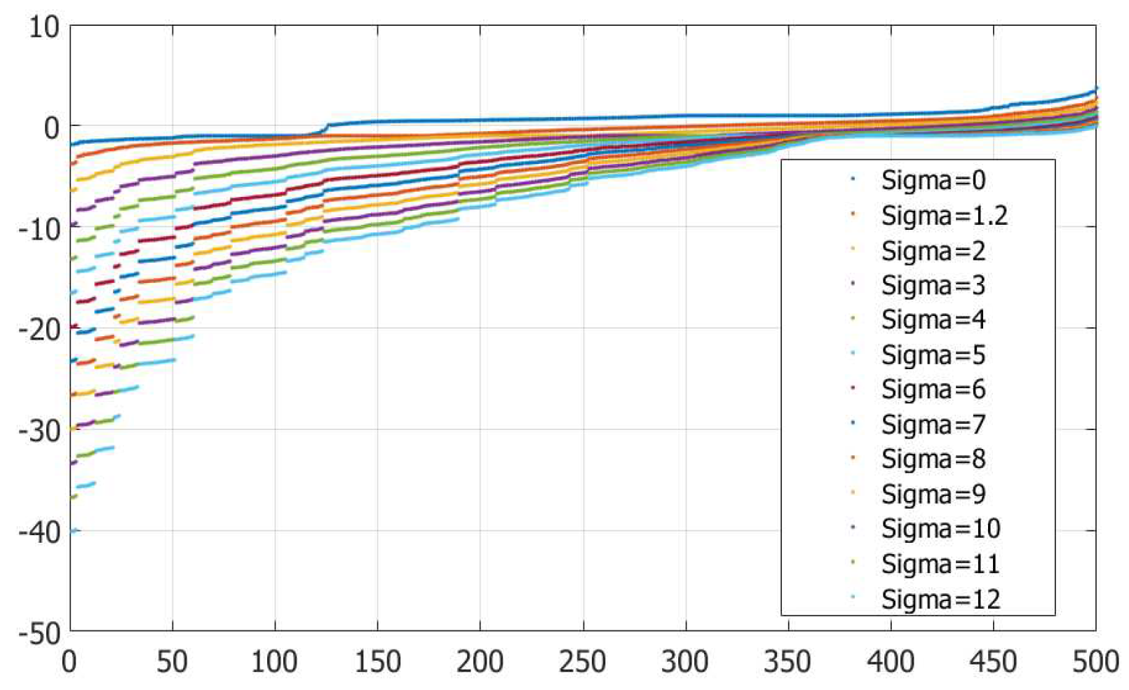
Figure 3.
Exact solution (blue dots) and Ritz values (red circles) computed by the SI Lanczos method + SYMMLQ with
Figure 3.
Exact solution (blue dots) and Ritz values (red circles) computed by the SI Lanczos method + SYMMLQ with
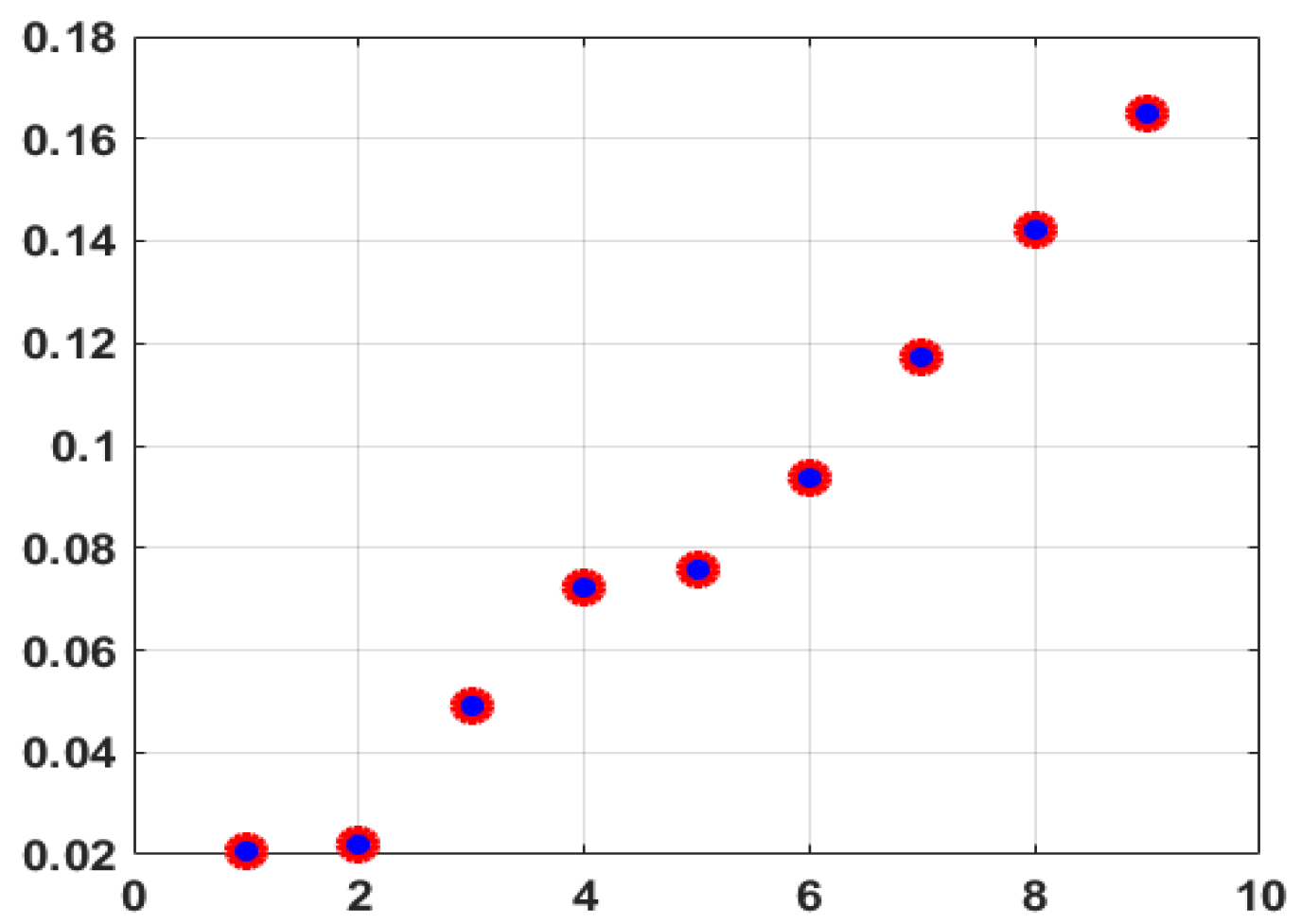
Figure 4.
The Ritz values (blue circles) and MATLAB solution (red dots) computed by the Lanczos method without shift and inversion for
Figure 4.
The Ritz values (blue circles) and MATLAB solution (red dots) computed by the Lanczos method without shift and inversion for
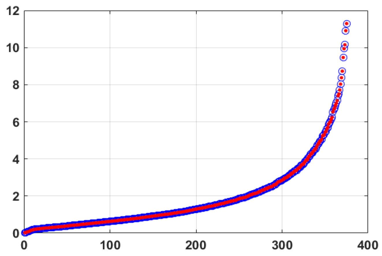
Figure 5.
Block-banded stiffness matrix (left) and mass matrix (right), , with nonzero elements.
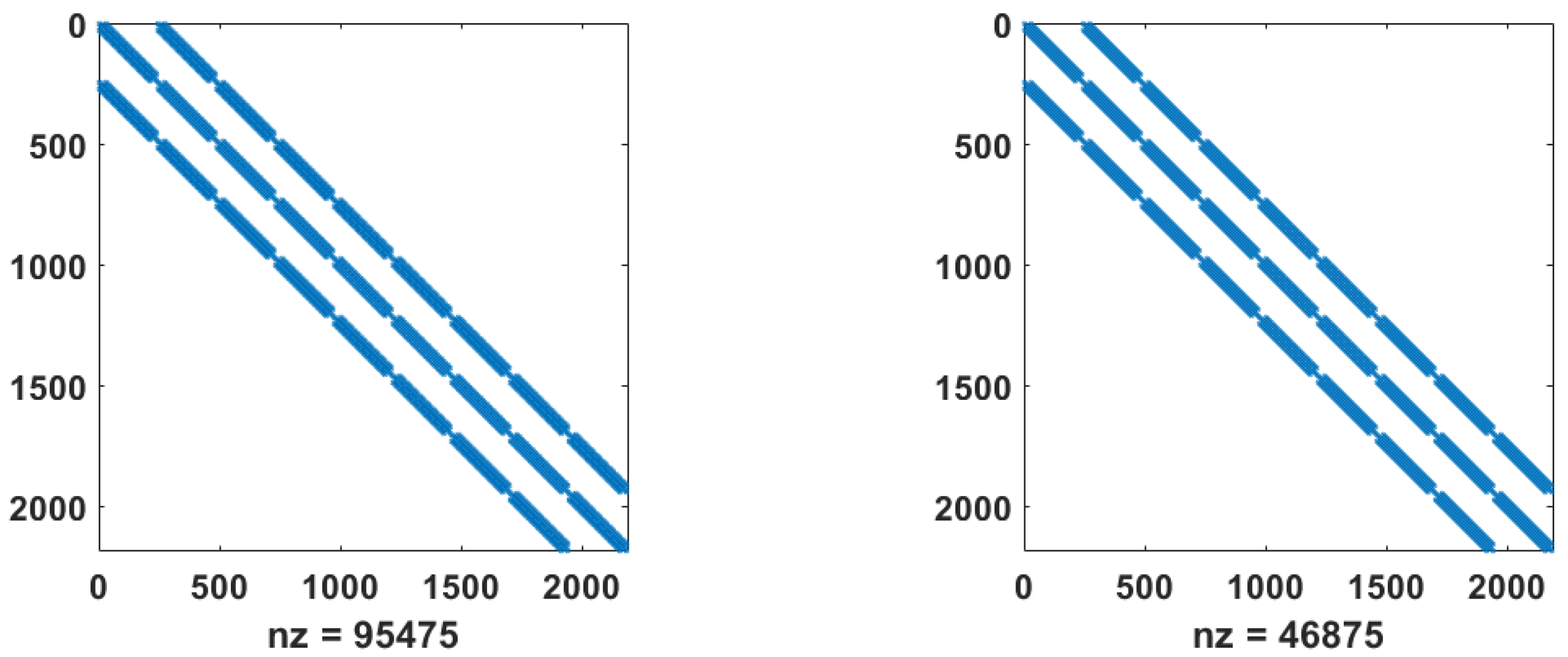
Figure 6.
Piezo transducer geometry in 3D (left) and deformed shape for the first resonance frequency
Figure 6.
Piezo transducer geometry in 3D (left) and deformed shape for the first resonance frequency
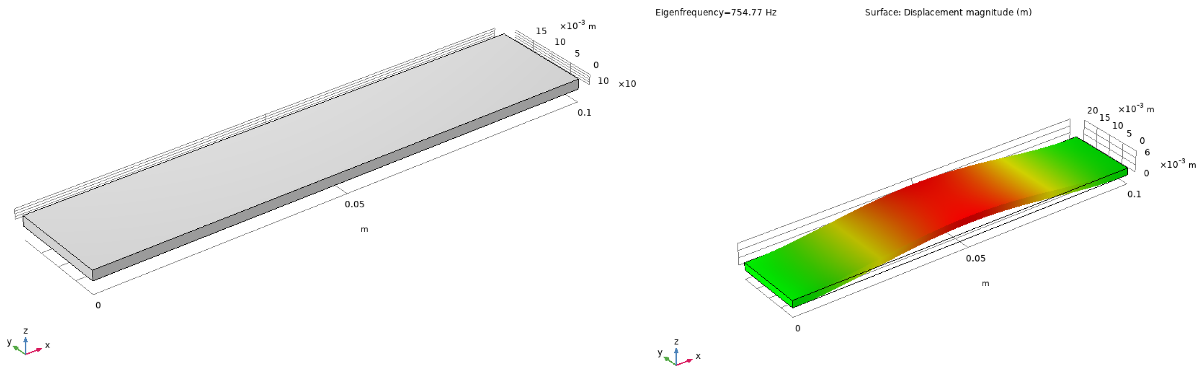
Figure 7.
Regular meshes with cubical (left, mesh A) and hexagonal (right, mesh C) elements
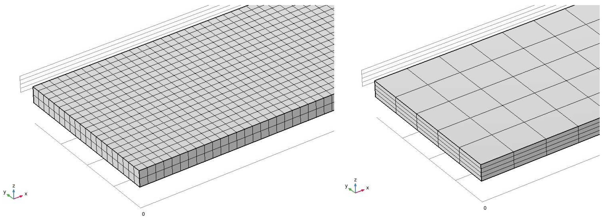
Figure 8.
Stiffness matrix structure for mesh A (left) and mesh C (right)
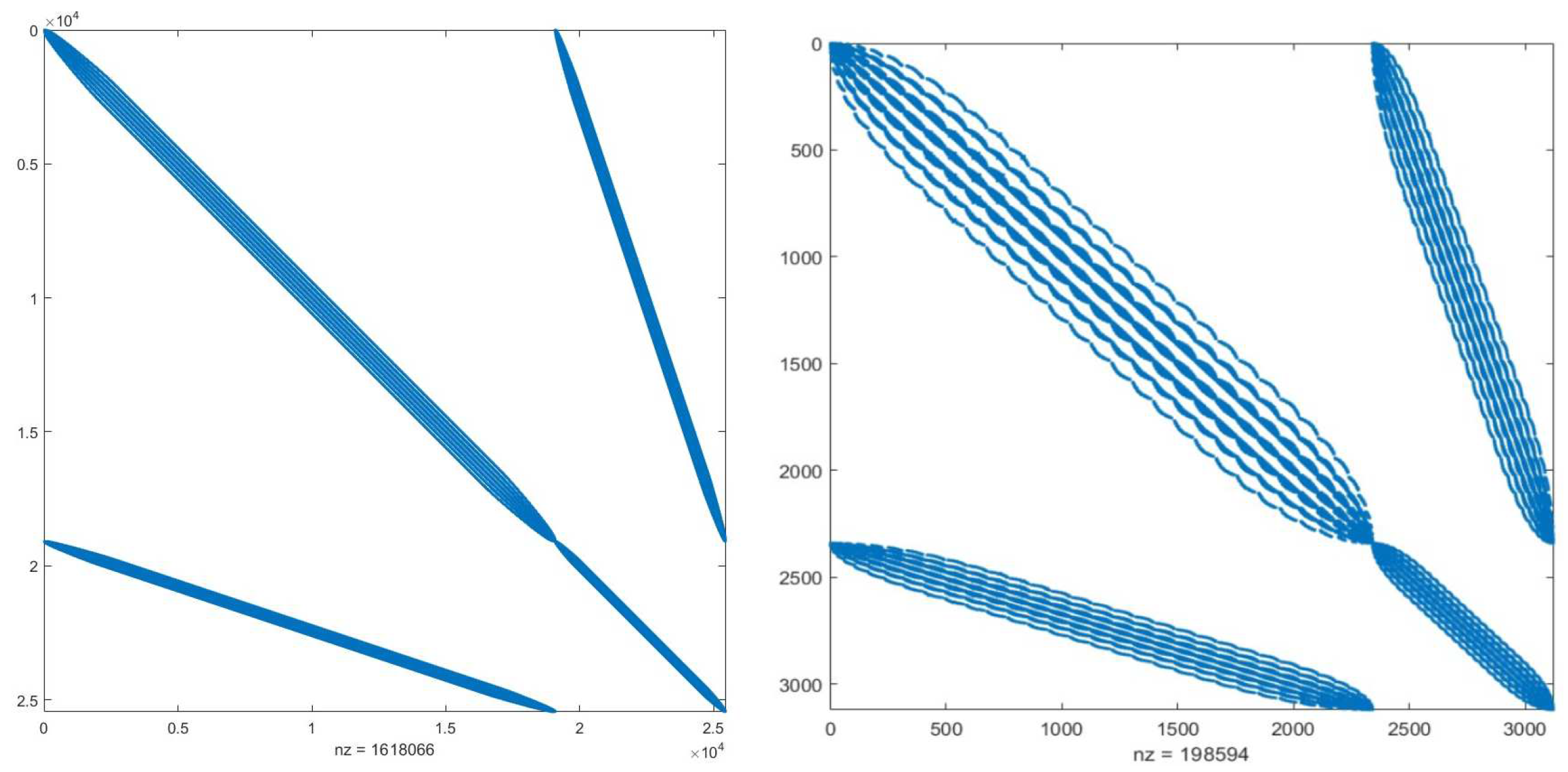

Table 1.
The MATLAB-solution , the Ritz values and modulo differences with computed by SI Lanczos + PSTS.
Table 1.
The MATLAB-solution , the Ritz values and modulo differences with computed by SI Lanczos + PSTS.
| N | |||
|---|---|---|---|
| 1 | 2.07409134398e-02 | 2.07409128594e-02 | 5.80390450977e-10 |
| 2 | 2.18457367533e-02 | 2.18457372638e-02 | 5.10444100182e-10 |
| 3 | 4.92520568661e-02 | 4.92520578446e-02 | 9.78553293951e-10 |
| 4 | 7.21956868830e-02 | 7.21956932561e-02 | 6.37314023776e-09 |
| 5 | 7.59552813845e-02 | 7.59552669848e-02 | 1.43997318235e-08 |
| 6 | 9.36225434064e-02 | 9.36225505277e-02 | 7.12121402124e-09 |
| 7 | 1.17174683420e-01 | 1.17174683147e-01 | 2.73150363439e-10 |
| 8 | 1.41972410416e-01 | 1.41972419018e-01 | 8.60313098538e-09 |
| 9 | 1.64801895988e-01 | 1.64801890736e-01 | 5.25220533731e-09 |
Table 2.
SI Lanczos + PCGNE, r is the matrix pencil dimensions, is the smallest eigenvalue, is the Ritz value and modulo differences.
Table 2.
SI Lanczos + PCGNE, r is the matrix pencil dimensions, is the smallest eigenvalue, is the Ritz value and modulo differences.
| n | r | IT | |||
|---|---|---|---|---|---|
| 500 | 375 | 18 | 2.07409131e-02 | 2.07409153e-02 | 1.9999998e-09 |
| 1000 | 750 | 23 | 2.07409143e-02 | 2.07409167e-02 | 1.5613999e-09 |
| 1500 | 1125 | 36 | 2.07410232e-02 | 2.07410426e-02 | 1.9419601e-08 |
| 2000 | 1500 | 42 | 2.07410259e-02 | 2.07410492e-02 | 2.4054199e-08 |
| 2500 | 1875 | 49 | 2.07410261e-02 | 2.07410521e-02 | 2.6000001e-08 |
Table 3.
Number of the nonzero elements (nz) in the ILU (LU) Crout factorization for matrices and error norm.
Table 3.
Number of the nonzero elements (nz) in the ILU (LU) Crout factorization for matrices and error norm.
| m | nz(ILU(A)) | nz(LU(A)) | norm(A - ILU(A)) | |
|---|---|---|---|---|
| 500 | 250000 | 16570 | 116734 | 3.1315129e-12 |
| 625 | 390625 | 24993 | 184672 | 3.4004757e-12 |
| 2187 | 4782969 | 95495 | 1067985 | 4.5358656e-10 |
| 3125 | 9765625 | 120983 | 2504612 | 1.1294766e-09 |
Table 4.
SI Lanczos + Crout ILU,
| N | |||
|---|---|---|---|
| 1 | 0.020740913439873 | 0.020740913439873 | 0.000000000000000 |
| 2 | 0.021845736753381 | 0.021845736753381 | 0.000000000000000 |
| 3 | 0.049252056866129 | 0.049252056866130 | 0.000000000000000 |
| 4 | 0.072195686883052 | 0.072195686883052 | 0.000000000000000 |
| 5 | 0.075955281384575 | 0.075955281384575 | 0.000000000000000 |
| 6 | 0.093622543406488 | 0.093622543406489 | 0.000000000000000 |
| 7 | 0.117174683420674 | 0.117174683488112 | 0.000000000067438 |
| 8 | 0.141972410415749 | 0.141973781586116 | 0.000001371170367 |
| 9 | 0.164801895988332 | 0.164863405361276 | 0.000061509372944 |
Table 5.
Numerical results for different meshes
| A | B | C | |
|---|---|---|---|
| Elements | 4000 | 32000 | 500 |
| Nodes | 6363 | 41205 | 780 |
| Degrees of Freedom | 25452 | 164820 | 3120 |
| Assembling Time, s | 4.12 | 23.28 | 1.28 |
| Matrix-Vector Prod, ms | 2 | 10 | Below 1 |
Disclaimer/Publisher’s Note: The statements, opinions and data contained in all publications are solely those of the individual author(s) and contributor(s) and not of MDPI and/or the editor(s). MDPI and/or the editor(s) disclaim responsibility for any injury to people or property resulting from any ideas, methods, instructions or products referred to in the content. |
© 2023 by the authors. Licensee MDPI, Basel, Switzerland. This article is an open access article distributed under the terms and conditions of the Creative Commons Attribution (CC BY) license (http://creativecommons.org/licenses/by/4.0/).
Copyright: This open access article is published under a Creative Commons CC BY 4.0 license, which permit the free download, distribution, and reuse, provided that the author and preprint are cited in any reuse.


