
Submitted:
16 November 2023
Posted:
17 November 2023
You are already at the latest version
Abstract
In space application, hybrid pixel detectors of the Timepix family have been considered mainly for measurement of radiation levels and radiation dosimetry in low earth orbits. By the example of the Space Application of Timepix Radiation Monitor (SATRAM), we demonstrate the unique capabilities of Timepix-based miniaturized radiation detectors for particle separation. Using a novel method for proton spectrum reconstruction, we were able to measure the spectrum of protons trapped in the inner Van-Allen radiation belt, for the first time with a single-layer detector. We assess the measurement stability and the resiliency of the detector to the space environment demonstrating that, even though degradation is observed, data quality has not been affected significantly over more than 10 years. Based on the SATRAM heritage and the capabilities of the latest-generation Timepix-series chips, we discuss their applicability for use in a compact magnetic spectrometer for deep-space mission or in the high radiation environment of the Jupiter radiation belts, and their capability for use as single-layer X- and γ-ray polarimeter. The latter was supported by measurement of the polarization of scattered radiation in a laboratory experiment, where a modulation of 80% was found.
Keywords:
Space weather
; scatter polarimeter
; hybrid pixel detectors
; Timepix
; dE/dX spectrometer
; low earth orbit
; magnetic spectrometer
; galactic cosmic rays
; space instrumentation
1. Introduction
Hybrid pixel detectors (HPD) of Timepix [1,2] technology have become increasingly interesting for radiation monitoring applications in space science. While up to date, common space radiation monitors rely on silicon diodes, achieving particle (mainly electron and proton) separation by pulse-height analysis, detector stacking, shielding or electron removal by a magnetic field, the key advantage of HPDs is that, in addition to the energy deposition measurement, particle signatures in the sensor are seen as tracks with a rich set of features. These track characteristics can be exploited for identification of particle type, energy, and its trajectory. Determining these pieces of information on a single layer bypasses the need for sensor stacking or complex shielding geometries, so that HPD based space radiation devices provide science-class data with a large field of view at an order of magnitude lower weight and approximately half of the power consumption compared with commonly used space radiation monitors.
While from 2012, Timepix has been utilized in Radiation Environment Monitors on-board ISS [3], the first Timepix (256 × 256 pixels, 55 µm pitch) used in open space is SATRAM (Space Application of Timepix Radiation Monitor) [4]. It is attached to the Proba-V satellite which was launched to Low Earth Orbit (LEO, 820 km, sun-synchronous) in 2013 and has celebrated 10 years in orbit in May, 2023. During this time, it has been providing data for mapping out the fluxes of electrons and protons trapped in the Van-Allen radiation belt, e.g., by in-orbit maps of the ionizing dose rate dominated by electrons in polar horn regions, as well as protons in the South Atlantic Anomaly (SAA) [5,6,7].
Over the years, different data analysis techniques have been successfully used for evaluation of the complex data set: Analytic categorization relying on extraction of manually defined track features, as well as novel machine learning approaches [7,8,9]. The success of SATRAM initiated the development of advanced miniaturized space radiation monitors, based on Timepix3 [10] and Timepix2 [11] technology. These are currently flown on the SWIMMR-1 (Space Weather Instrumentation, Measurement, Modelling and Risk) [12] mission (launched in 2023) and shall be used within the European Radiation Sensor Array (ERSA) [13].
Large area Timepix3 detectors (512 × 512 pixels, 55 µm pitch) were developed for the demonstrator of the penetrating particle analyzer [14] (Mini.PAN), a compact magnetic spectrometer (MS) designed to measure the properties of cosmic rays in the 100 MeV/n–20 GeV/n energy range in deep space with unprecedented accuracy, thus providing novel results to investigate the mechanisms of origin, acceleration and propagation of galactic cosmic rays and of solar energetic particles, and producing unique information for solar system exploration missions. Precise per-pixel time measurement together with a high spatial segmentation allows its use a single-layer Compton camera, thus making it an interesting tool for directional hard X- or -ray detection and polarization measurement in space.
2. Materials and Methods
2.1. Timepix series
Among the different readout ASICs developed in the Medipix collaborations, the Timepix series: Timepix [1], Timepix2 [11], Timepix3 [2] and Timepix4 [15] were dedicated to single-particle detection and tracking.
Timepix was developed within the Medipix2 collaboration [16]. It segments the sensor into a square matrix of 256 × 256 pixels with a pixel pitch of 55 µm and purely relies on a frame-based readout scheme (dead-time >11 ms). Each of the 65,536 pixels can be set to either of the three modes of signal processing: Time-over-Threshold (ToT), Time-of-Arrival (ToA, resolution >10 ns) and hit counting. Timepix2, while still relying on the frame-based readout, provides additional features: e.g., a simultaneous measurement of ToA and ToT, and an adaptive gain ToT mode for improved spectroscopy at high energy deposition [17]. The key improvements of Timepix3 are a time resolution below 2 ns and the data-driven mode. The latter one hereby provides an almost dead-time free detector operation by reading out only the pixels which are actually triggered by an ionizing particle, while all other pixels remain active (per-pixel dead: ∼475 ns). Pixel hit rates up to 80 MHits s−1 can be send off chip at a bandwidth of 5.12 Gbps.
Timepix4 comes with an increased pixel matrix featuring 512 × 448 pixels with a pitch of 55 µm (resulting in an area of ∼7 cm2) [15]. Similar to Timepix3, it offers frame-based and data-driven readout schemes, but with 8 x higher maximal hit rate. The time binning is improved to 195 ps. The readout bandwidth can be up to 164 Gbps.
The ASICs can be coupled to different sensor materials by means of flip-chip bump bonding. Currently available and tested sensor materials are silicon, CdTe, CZT and high resistivity chromium compensated GaAs:Cr with thicknesses ranging from 100 µm to 2 mm. Improvements in growth techniques facilitate the availability of thick sensors with low defect density (CdTe, GaAs:Cr, CZT), which profit from a higher -ray detection efficiency and single layer tracking performance. Readout systems for Timepix, Timepix2 and Timepix3 have been developed in the Medipix/Timepix community relying on different communication protocols (see e.g., [18]).
2.2. The Space Application of Timepix Radiation Monitor (SATRAM)
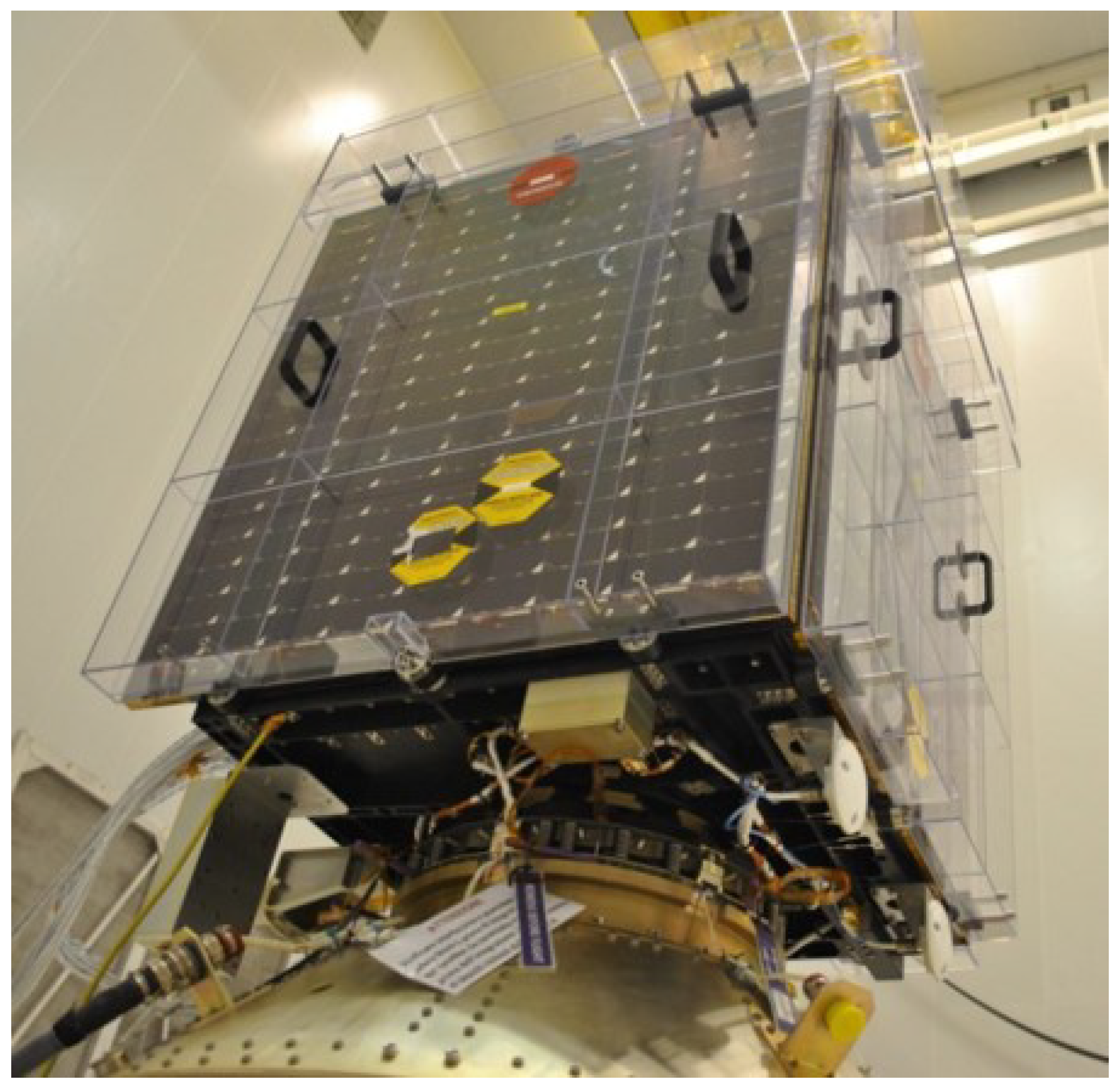
The first application of a Timepix in open space was SATRAM (Space Application of Timepix Radiation Monitor) on board the Proba-V satellite launched in May, 2013. The satellite is orbiting Earth in a Sun-synchronous orbit at an altitude of 820 km with an inclination of 98.7°. The orbit duration is 101.21 min and the local time at descending node is between 10:30 a.m. and 11:30 a.m.. The SATRAM module is encapsulated in an aluminium alloy compartment. It has a thinned area above the sensor with a thickness of 0.5 mm. The module weighs 380 g, has a power consumption of 2.5 W and dimensions of 55.5 × 62.1 × 197.1 mm. The Timepix inside the module hosts a 300 µm thick silicon sensor. The threshold is globally set to 8 keV. The detector is operated in ToT-mode with acquisition times for consecutive frames set to 20 s, 200 ms, and 2 ms to account for the different flux-levels in orbit.
Figure 1.
Picture of SATRAM attached to Proba-V.
SATRAM’s continued operation allowed measurements of fluxes of electrons and protons trapped in the Van-Allen radiation belts continuously during its ongoing mission. Current proton and electron separation relies on pattern recognition together with the dE/dX information. Recent work started to use convolution neural networks (CNNs) to improve classification accuracy [8]. Based on the success of SATRAM, proposals to develop a Miniaturized Radiation Monitor (MIRAM) [10] and the Highly Integrated Timepix-based radiation monitor (HITPix) have been funded by the European Space Agency (ESA). The major differences that set these detectors apart from other commonly used radiation monitors like ICARE [19,20] or the Standard Radiation Environment Monitor (SREM [21,22] are single-layer particle discrimination capabilities, which allow for development of radiation monitors of small dimensions, low mass with a large field of view.
2.3. Pattern recognition tools and particle separation
Detectors of the Timepix family are sensitive to a broad variety of particle species: from X-rays and electrons with energies just above 3 keV up to particles in the GeV range. The detector segmentation, together with the charge transport properties of its semiconductor sensor create imprints in the pixel screen (clusters or tracks), which are to some extend usable for particle identification.
A basic pattern recognition scheme was introduced in [23] in 2008. It defines six categories of events: dots, small blobs, curly tracks, heavy blobs, heavy tracks, and straight tracks, each indicating different particle species and energy deposition shown in Figure 2. This methodology purely relies on the track morphology. Additionally, Timepix allows the use of the energy information, with which properties like the deposited energy, cluster height (energy of the highest energy pixel in a cluster) and the stopping power can be determined. Timepix can also provide timing information, but not while simultaneously measuring the energy. This ability was added in subsequent generations with Timepix2 and Timepix3. Together with increased energy resolution, the particle recognition capability was thus improved.
A first attempt to identify particle species in radiation fields in space utilizing Timepix technology was done in [6] using SATRAM data. Here, electrons and protons are the most abundant particle species. The most significant properties used in this work were the track morphology from [23] mentioned before, cluster height and stopping power. Monte Carlo simulations showed that for electrons the cluster height is not higher than 300 keV and the stopping power is not more than 10 MeV cm2/g. The simulations were done for spectra that are expected in the radiation belts, so for electrons with energies up to 7 MeV and protons with energies up to 400 MeV. While accurately determining electrons (correct classification in 98%), this method falls short in the identification of protons. High energy protons (>100 MeV) have a significant lower energy deposition and stopping power which is on par with electrons. Especially protons that pass through the detector perpendicularly, and thus creating only a short track, would often be misidentified as electrons.
The next step was to apply neural networks to improve particle identification. The first successful use was from [8]. It used fast Monte Carlo simulations that created simplified particle tracks for training of a CNN. In the simulation, all particle tracks were only one pixel in width. While electron track are seldom wider than one pixel, proton tracks are usually two to four pixels wide. However, it was shown that neural networks can be successfully used for particle identification in the case of electron and proton dominated space radiation data. It was even shown that spectroscopic information for protons at lower energies (<50 MeV) can be extracted.
After improving Monte Carlo simulations for Timepix data to also include charge sharing effects (i.e., creating wider particle tracks for protons), another iteration of the NN was developed [7]. This feedforward neural network created in the TensorFlow framework [24] uses seven features to classify a cluster:
- the number of pixels in the cluster N;
- the deposited energy is defined as the sum of energies measured in the pixels of a cluster ;
- the maximal energy measured in a single pixel of the cluster ;
- the linearity of the cluster, defined as the relative amount of pixel lying within a distance of one pixel from the longest line segment between two pixels of the cluster;
- the roundness of the cluster;
- the average number of neighbouring pixels;
- the sum of the absolute values of cubic and quadratic terms of a third order polynomial fit of the cluster.
The NN consist of an input layer, two hidden layers with seven neurons each, and one output layer. An overall testing accuracy of 90.2% was achieved, with protons being correctly classified in 89% and electrons in 91% of cases. In orbit, proton fluxes are still difficult to determine accurately, given that electron fluxes are often higher by about two orders of magnitude and electrons falsely identified as protons are of the same order of magnitude as the protons.
For the NN to work properly, it is required that clusters are well separated from each other. However, particle tracks inevitably overlap, when frames have longer acquisition time and/or the fluxes are high. The NN is not able to recognize the two or more tracks, let alone identify what particle species they are. To quantify this effect, the occupancy has been introduced. It is calculated by the number of hit pixels divided by the number of available pixels. The result is expressed in percent. To ensure that the NN can work properly, only frames with a maximum occupancy of 20% were selected (low occupancy frames). For frames with higher occupancy (high occupancy frames) a different method had to be applied.
To estimate the electron fluxes of high occupancy frames, a more statistical approach was chosen. The first step was to determine a mean energy of all clusters depending on the geographical position of the current measurement. The information was obtained by looking at the low occupancy frames in the region and calculate a mean energy for all particle tracks that were measured in the area. Typically, this local mean energy is higher in the SAA than the rest of the orbit due to the abundance of protons in that region. The estimation of the number of particles in the frame was then obtained by dividing the total measured energy in the frame by the local mean energy corresponding to the position of the satellite and then multiplying this by the fraction of electrons, known from the previous low occupancy frame. Both methods were explained in detail in [7].
2.4. dE/dX spectrum unfolding
Spectrum deconvolution refers to the decomposition of a complex signal into its contributing spectrum components. There are many different iterative and statistical schemes that can be chosen for this process. For this paper, the Bayesian deconvolution scheme was been chosen [25], which utilises the Bayesian probability formula:
where p represents a generic probability function, | the given operator, and A and B some arbitrary variables or system states. Despite the simplicity of the Bayesian formula it is quite powerfully and used in many areas of physics and statistics. The formula conveys the probability of A having a particular value or state given that B has a particular value or state, essentially relating two otherwise unrelated states. The states A and B can be assigned some arbitrary distribution of two variables that will be referred to as the cause vector () and the effect vector (). It can then be assumed there exists an arbitrary probability distribution given by the formula
The approximate values of can be achieved through simulation. The remaining probability values for a specific experiment can be obtained through the Bayesian iterative deconvolution algorithm that is implemented using the library [26].
To use the Bayesian deconvolution algorithm, an incoming spectrum () is related to the measured spectrum () in a so-called “response matrix”. In the present work, the response matrix relates dE/dX spectra to an incoming mono-energetic electron or proton field (Figure 3). Therefore, for each detected track the stopping power was calculated as:
with the per-pixel energy of a particle trace , the sensor thickness = 300 µm, the density of silicon g cm−3, and the reconstructed impact angle with respect to the sensor normal . The latter was determined as described in [27]. Accounting for the expected particles and energies, the response spectra were simulated in electron primary energy bins and proton primary energy bins with a flat distribution from 0 to 10 MeV and 0 to 500 MeV, respectively, using the Allpix Squared simulation framework [28]. It is worth noting that all electrons MeV are degenerate and protons are asymptotically electron-like with increasing energy.
2.5. 3D reconstruction of particle traces within the semiconductor sensor - the use as a solid-state time-projection chamber
Ionizing radiation interacting in the sensors creates free charge carriers, which start to drift towards the electrode of opposing charge. During this drift motion, currents are induced at the pixels in close vicinity. Due to the small pixel size compared to sensor thickness, detectable signals are only induced if the charge carriers are close to the pixel side (small pixel effect), so that the measured time corresponds approximately to the drift time across the sensor thickness.
The charge carrier (electrons e and holes h) drift along the z-axis of the device can be described by
where is the mobility of electron and holes, respectively. For planar silicon sensors in hole collection a linear parameterization of the electric field can be used:
where d denotes the sensor thickness, is the bias voltage and is the depletion voltage. While depends on the quality of the sensor and should be determined individually, we can use as a rule of thumb. For semi-insulation planar sensors (CdTe, CZT, and GaAs:Cr) with ohmic contacts, we assume a linear electric field across the sensor thickness
While the charge carrier drift motion can be described analytically, the induction process requires numeric calculation (iterative simulation). Therefore, the charge carrier drift motion and the amount of deposited charges were considered to create a look-up table relating the energy deposition and measured time stamp to the interaction depth (see [29]).
2.6. Single-layer Compton camera and scatter polarimetry
Fine pixelation and 3D reconstruction within the sensor allows the use as a single-layer Compton camera. Therefore, the Compton electron has to be detected together with the scattered X-ray photoelectron. With the Compton electron detected at depositing energy and the scattered photon detected at with energy , we can define Compton cones around the axis defined by the directional vector with tips located at [32]. The opening angle is given by
with keV being the electron rest energy and [32].
Polarized incoming radiation will create an asymmetry in the scattering angles evaluated in the detector pixel plane. Compton scattering differential cross section for a single X-ray photon is described by Klein-Nishina formula [33]
where m is the classical radius of electron, is the angle of the outgoing photon with respect to the direction of the incoming photon and is the angle between scattering plane and polarization plane. The scattered photon preferentially flies perpendicularly () to the polarization of the incoming photon.
A concurrent detection of Compton electron with photoelectron therefore allows for X-ray polarimetry. We take the detector’s x-axis as reference and determine the angle as where is the x-axis unit vector. For partially polarized photon impact, the scattering angles will be distributed as
where A is a scaling factor, is modulation, and phase determines the polarization direction of the incoming X-rays with respect to x-axis. Here we assumed that our detector is equally sensitive in all azimuthal directions . The degree of polarization is then
where denotes the modulation response to a 100% polarized X-ray impact, which can be calibrated in simulation [34] or in a field of known polarization.
3. Results
3.1. Space heritage - SATRAM and its 10 years of operation as a radiation monitor
3.1.1. Measurement stability - noisy pixel appearance and removal
In this section, the state of SATRAM in terms of radiation induced effects on data quality shall be quantified. This will be done by looking at the amount of noisy pixels that may occur over time in a different quantity. Noisy pixels are defined as pixels exceeding the overall countrate statistically significant. While most of the identified noisy pixel were recoverable and dissappeared after resetting the detector configuration, some became permanently noisy. The latter, were masked (removed from the data set) and, thus, are not considered in the analysis. Given that there are 65,536 pixels, the loss of a few hundred pixels is negligible for the overall data quality.
To determine if a pixel is noisy one usually takes an arbitrarily high number of frames and counts how often a each pixel has send a signal. In the case of this study, the noisy pixel search was done on the time-scale of 1 week. The number of counts measured in each of the pixels within this time period are registered in a histogram. The resulting distribution was then fitted with a Gaussian distribution, obtaining the mean and the standard deviation . We define the threshold for a pixel to be considered as noisy, , as
This procedure was done for every consecutive week from the beginning of available data in August, 20141, until the 30th of June, 2023. Furthermore, this analysis was done separately for the three different acquisition times. Naturally, more pixels will have sent a signal in longer frames than in shorter ones, which could have skewed the distributions. The resulting relative numbers of noisy pixels are shown in Figure 5.
It can be seen that the number of noisy pixels until the end of 2021 are below 0.6%. In 2021, there are two increases over a few weeks in spring and autumn. The same can be seen for the year 2022, but with significant increase in the number of noisy pixels. No definite explanation has been found for the increase nor for the periodicity.
In 2023, the detector seems to have recovered. A careful inspection of the data has shown that most of the data is measured as expected. There are a few cases, where the matrix gets filled up to a large portion, while being in the corresponding region of space where no high fluxes of radiation are expected. While the statistical method for noisy pixel determination used here is not suitable to detect this kind of behavior, these frames stand out and were excluded from analysis by comparison of their count rates with previous and subsequent frames.
The distribution of noisy pixels over the pixel matrix can be seen in Figure 6 for the years 2015 on the left and 2022 on the right. In 2015, most noisy pixels are concentrated in the lower left corner. This is a well-known firmware issue of SATRAM and was present already from the beginning.
These pixels have been excluded from analysis in all previous studies. In 2022, the pixels in the lower left corner are still noisy and seem to have worsened. Additionally, pixels along the edge are showing increased noise behaviour. The edge pixels being noisy can be observed in many frames acquired in 2022. However, their position makes it easy to mask them and eliminate them from analysis. Their exclusion results in reduction of the usable detector area by 21%.
A follow up analysis, using the same method for noisy pixel detection, but for a reduced number of pixels has been done. The noisy pixels in the lower left corner and the edge pixel as seen in Figure 6(b) has been masked (excluded). The result is presented in Figure 7. The number of noisy pixels were greatly removed to below 0.2%, except for a short period in late 2022, where about 10% of pixels were identified as noisy. This effectively shows that by reducing the active area of the sensor through masking the problematic areas, SATRAM provides reasonable data during its entire 10 years of operation.
3.1.2. Mapping out electron and proton fluxes in orbit
Figure 8(a) and 8(b) show the fluxes of electrons and protons classified with the method described in Section 2.3. The majority of particles present in the radiation environment in LEO are protons (up to 400 MeV) and electrons (up to 7 MeV) that are trapped by the Earth’s magnetic field. For electrons, three distinct structures are discernible, i.e., the northern polar horn, the southern polar horn, and the South Atlantic Anomaly (SAA). The northern and southern polar horns correspond to the points at which the satellite passes through the Earth’s outer radiation belt. The SAA is present due to the satellite crossing the Earth’s inner radiation belt. This crossing is possible due to the incline of the Earth’s magnetic dipole combined with the deviation of the Earth’s magnetic centre with respect to the Earth’s centre of mass. While the outer radiation belt consists of electrons, the SAA is the only area in SATRAM’s orbit, where a non-negligible flux of protons should be present. Thus, protons seen in the polar horns (in Figure 8(b)) are interpreted as misclassified electrons.
3.1.3. Measurement of the proton spectrum in the SAA
Figure 9(a) shows the spectrum reconstructed for the central region of the SAA. Therefore, frames with occupancy <5% recorded within the area defined by longitude and latitute were selected. The occupancy cut is required to reduced the probability of track overlap resulting in improper determination. During 2016-2018 operation, the total effective measurement time was 92 s.
Applying the unfolding methodology defined in Sec. 2.4 to the measured spectrum, we find the yellow curve in Figure 9(b). To understand the energy dependent “background” contribution of electrons, the methodology was applied to simulated data. Therefore, the expected electron spectrum was extracted from SPENVIS [35] using AE-8 MIN [36] and used as input for detector response modelling with Allpix2 [28]. The output of the simulation is processed in the same way as the measured data finding the blue curve in Figure 9(b). The electron contribution becomes visible for the energy region above MeV and dominates the count rate above ∼140 MeV. The final proton energy spectrum presented in Figure 9(c) was obtained by bin-wise subtraction of the measured and the simulated electron-background spectra.
3.2. Large area Timepix3 detectors as tracking modules in a magnetic spectrometer
The development of a penetrating particle analyzer (mini.PAN) started in January 2020 in collaboration with the Department of Nuclear and Particle Physics (DPNC), University of Geneva and the National Institute of Nuclear Physics (INFN), Perugia Section. Mini.PAN employs position-sensitive (pixel and strip) detectors and (fast) scintillators to infer the particle type and velocity of GeV particles (and antiparticles) passing through the instrument’s magnetic field by measuring their bending angles, charge deposition and time-of-flight. Once in orbit this device allows a precise measurement of flux, composition, spectral characteristics and directions of penetrating cosmic-rays and antimatter searches over the full solar cycle. While such measurements exist within the heliosphere, Mini.PAN is designed as a compact instrument with low mass operating at low power. Thus, it will allow use in deep space or on smaller satellites. Figure 10a) shows the developed pixel module featuring 4 Timepix3 detectors in a 2 × 2 geometry (quad), giving a 7.92 cm2 area with 262,144 pixels at a pixel pitch of 55 µm. Figure 10b) shows the pixel module integrated into the demonstrator.
Figure 11 shows tracks and the stopping power spectra measured with the developed device at different angles within a relativistic hadron beam (90% pions), measured at the CERN SPS. The distributions are modelled as the convolution of a Landau curve, describing the physics the particle energy loss in the sensor, smeared with a Gaussian, whose width indicates the detector’s energy resolution. Rotation of the device allows to study this resolution at different deposited energy. We find keV (), keV () and keV ().
A detailed study of the temperature influence on the device performance and different operational parameters providing low power operation have been presented [37]: In the best case, a power consumption of ∼2 W for the entire quad was achievable.
3.3. Capabilities of Timepix3 as a Compton camera and scatter polarimeter
The capabilities of a single-layer Timepix3 for use as a Compton polarimeter, was studied in a laboratory experiment. The experimental setup is shown in Figure 12(a). X-rays from a Hamamatsu microfocus tube were collimated onto a relatively large plastic target (dimensions: cm3) placed at a distance of 21.5 cm to the collimator. The tube voltage was set at kV with a tube current of µA. A 1 mm thick pixelated silicon sensor (55 µm pixel pixel pitch) attached to Timepix3, reverse biased at 400 V, was used to detect the scattered X-rays.
The detector was placed at 16 cm from the target in a way that the X-rays of the highest degree of polarization (scattering off the target at 90°) can be recorded. Using the detector in data-driven operation, we search for coincidentally detected pairs of clusters using a floating time window of ns (drift time of holes across the whole thickness of the sensor). We refer to a set of coincidentally detected clusters as “coincidence group”. Coincidence groups larger than 2 clusters were omitted from the analysis. The cluster with higher energy in each coincidence pair was assumed to be a photoelectron deposited by the scattered photon, while the lower energies are assigned to Compton electrons. The incoming photon energy is reconstructed by summing the two energy measurements . Using Eq. (8), we calculate cosine of the scattering and select only pairs with .
We can apply further cuts to achieve as high modulation as possible while retaining enough statistics. A cut on pixel plane distance between the clusters has been found producing modulation around . Figure 13 shows the measured scattering angle distributions fitted with Eq. (10), showing also the modulations and phase shifts found by fitting. In order to demonstrate that the seen modulation is in fact an effect observable in the laboratory frame and not inherent to the technology, the detector was rotated around the axis defined by the target and detector. The observed phase shifts are consistent with the angle offsets. Histogram of energies of the selected clusters is in Figure 12(b). Clusters labelled as Compton electrons and photoelectrons are well separated. There are no Compton scattering clusters with energies keV due to per pixel detection threshold.
The minimal time () measured by a single cluster within a coincidence pair defines the time reference used for the calculation of the relative 3D coordinates (as described in Section 2.5). Figure 14 shows the Compton camera reconstruction using simple back projection with weighted cones. The empirical weight function favors cluster pairs with higher energy of Compton electrons (less uncertainty in ), absolute time of arrival difference being close to either ns or ns and large distance d (less uncertainty in cone axis vector).
4. Discussion
4.1. Timepix-based radiation monitors
In contrast to commonly used space radiation monitors, Timepix-based devices provide the capability to separate different particle classes with a single-layer detector. This allows the development of competitive low mass (∼100 g) radiation detectors which inherently provide an almost 4 field of view. In the present contribution, we have outlined these capabilities by the example of SATRAM, which has been operated in open space for more than 10 years.
While Timepix can be considered as a noise-free individual particle detector, due to single-event effects appearing in chip registers, individual pixels can “lose” their configuration becoming noisy until their configuration is reset [38]. Long-term irradiation additionally results in electronics baseline shifts, which could affect the noise behavior of the entire sensor. We have studied the appearance of noise patterns in the measured data by searching for outlier pixels with unphysically high count rate. For the first 8 years of operation, the number of such pixels was consistently on the level of 0.6%. During 2022 operation, the number of noisy pixels reached values of up to 22% and recovered in 2023. It was found that the noise level increase in particular affected pixels at the edges of the sensor, which were subsequently excluded reducing the relative amount of noisy pixels to 0.1% (with the exception of a short period in late 2022 with up to 10%). While the effectively used detector area had to be reduced by 21% for 2022 operation, the overall data quality and scientific reach of the detector was not affected.
The current limitation of SATRAM compared, e.g., with the Energetic Particle Telescope, was its insensitivity to resolve the spectral characteristics of the incoming radiation. Within in the present work, we have overcome this problem - at least for protons - using a novel spectrum unfolding methodology. For the first time, we were able to present a proton energy spectrum measured with a single-layer device in low earth orbit. Comparison of the obtained result with previous measurement and predictions is out of the scope of this work. The energy selective detection of electrons in the LEO radiation environment still remains unsolved, and should be addressed in future development, e.g., by implementing multi-detector devices of with sensors of differing stopping power or by adding electron stopping filters to the backside of the sensor.
A drawback of Timepix is that measurements are taken in frames of predefined acquisition times. Thus, at changing radiation fluxes, overexposure of frames occurs, leading to track overlap and misclassification of events. Selection of frames with low occupancy mitigated this issue at the cost of losing measurement time. This issue was addressed with the design of next generation Timepix ASICs. For example, Timepix2 provides “online” monitoring of the frame occupancy with automatic frame termination once a preset amount of columns is triggered; Timepix3 implements a data-driven mode, where only pixels triggered by radiation are read out all others remain active. The latter, however, comes with the possibility of high measured data rates. Considering typically limited resources for data storage and downlink, this imposes the requirement for an on-board data compression. Therefore, methodology and algorithms are needed which can analyse the data at low computing power. Development going in this direction has been started.
4.2. Towards astroparticle physics application
Highly spatially segmented detectors with decent time resolutions are a valuable asset also for astroparticle physics instrumentation. In contrast to the space weather and radiation dosimetry studies, where small detectors are beneficial, astrophysical observations usually require detectors of large area to cope with low flux rates.
4.2.1. From Mini.PAN to Pix.PAN
A Timepix3 quad detector was developed for application in Mini.PAN, which is a two-sector magnetic spectrometer proposed for an in-situ spectrally resolved measurement of the galactic cosmic ray fluxes. The developed detectors have an effective area of 7.92 cm, segmented in 262.144 pixel of 55 × 55 µm2. In the current instrument design they are mainly supplemental detectors adding high flux capabilities, an additional charge and position measurement. Their limited spatial (µm µm) and temporal resolution (∼2 ns), prevents them from being used as a standalone tracker (requirement: µm) or as a segmented time-of-flight module (requirement: ps). As outlined in [39], these issues can be overcome by the latest generation of Timepix-series chip, namely Timepix4, inherently providing a time granularity of ps, combined with an adapted sensor design using a “pitch adapter” to create rectangular pixels of µm area. The small pitch in bending direction is sufficient for measuring the curvature of particles in the range up to 10 GeV/c with the baseline Mini.PAN Halbach magnets of 0.5 T [14]. The lax requirement in non-bending direction further allows to save power by switching off 7/8 of the pixels. The production and testing of the novel sensor design has been started.
The Pix.PAN design relies on three tracking stations, each consisting of a stack of two Timepix4 quads [39]. While synchronization of 24 detectors at picosecond precision requires careful electronics design, relying on a single detector technology represent a significant simplification compared to Mini.PAN. The high-rate capability of Timepix4 will allow for application in harsh radiation environments, such as the Jovian radiation belts.
4.2.2. Compton scatter polarimetry
At last, we have presented a simple laboratory experiment demonstrating the capability of Timepix3 to be used as a single-layer Compton camera and scatter polarimeter. Therefore, we profited from the capability of reconstructing the locations of the interaction of ionizing radiation withing thick sensors in 3D enabled by nanosecond-scale drift time measurement. We measured the modulation for X-rays from a microfocus tube (tube voltage: 75 kV) scattered at 90 degrees in a plastic target to be . This represents an improvement of ∼29% compared with previous work [34] using Timepix in a similar experiment (finding a modulation of 62%).
To further understand the detectors capability, a simulation in Geant4 [40] with X-rays hitting a mm silicon sensor was carried out. Simulated X-ray beams were monoenergetic, non-dispersive, had a uniform spatial distribution, and were arriving at an angle of to the sensor plane. Three types of beams were simulated: unpolarized, 100 % polarized with polarization direction at , and 100 % polarized with the polarization vector oriented at to to the sensor’s x-axis. Only events with the photon interacting twice in the sensor were selected. The same cuts on and distance d were made as for the experimental data. Interactions with an energy deposit keV, resembling the per pixel energy threshold, were omitted. We find that for 100% polarization in the incoming photon energy range from 45 to 75 keV a modulation % could be achieved. Further simulation using a proper detector response simulation are the topic of future work. These will help to find optimized event selection criteria and obtain ground truth data samples as input for machine learning techniques.
We can further assess the performance of the device by the Minimum Detectable Polarization (MDP) at 99% confidence level, describing the degree of linear polarization detectable within a given acquisition time. Neglecting background, it can be estimated as [34]:
where is the number of detected scatter electron-photon pairs and the modulation measured at 100% polarized radiation. We can solve Eq. 13 for to estimate the minimal amount of detected scatter events
With % (from the simulation) and MPD%, we find .
The possibility to use different sensor materials of various thicknesses with the same Timepix readout ASIC hereby allows selection of sensors optimized for the desired photon energy range. The larger area and lower power density per unit area of Timepix4 will further enhance applicability for space research. Thus, future work should study the capabilities of thick CdTe (available up to 2 mm) and CZT (up to 5 mm [41]) devices for measurement in the hard X-ray band, terrestrial -flashes or -ray bursts.
5. Conclusions
In summary, we have demonstrated that Timepix-familiy detectors’ capability of single-layer particle tracking and particle species separation allows a production of competitive radiation monitors with one order of reduction in mass and covering almost the entire solid angle range. Application of novel methdology utilizing the Timepix3 time resolution for reconstruction of the z coordinate provides 3D reconstruction of particle tracks, which in “thick“ sensors enables their use as single-layer Compton camera and scatter polarimeter. Here, the possibility to combine the readout ASIC with sensors of different materials provides means of optimization for different X- and -ray bands. While currently Timepix3 detectors are integral part of particle spectrometers for measurements of galactic cosmic ray properties (Mini.PAN), the latest-generation Timepix4 could be baseline technology of future magnetic spectrometers adding high rate capability and electronics simplification (Pix.PAN).
Author Contributions
Conceptualization, B.B. (Benedikt Bergmann); Formal analysis, D.G (Declan Garvey), S.G. (Stefan Gohl), and J.J. (Jindřich Jelínek); Funding acquisistion, B.B., Investigation, J.J., Methodology, B.B., S.G., D.G. (Declan Garvey) and J.J.; Project administration, B.B., Resources, P.S. (Petr Smolyanskiy), Software, S.G., D.G. and J.J.; Supervision, B.B. and S.G., Validation, S.G., D.G. and J.J.; Visualization, S.G., D.G., and J.J.; Writing—original draft preparation, B.B.; Writing—review and editing, S.G., D.G., J.J., and P.S.; All authors have read and agreed to the published version of the manuscript.
Funding
This research was funded by the Czech Science Foundation under grant number GM23-04869M.
Data Availability Statement
All SATRAM data are available through the online tool https://satram.utef.cvut.cz/. Other presented data and used reconstruction codes are available upon request.
Acknowledgments
Successful launch and operation of SATRAM would not have been possible without Stanislav Pospíšil, Carlos Granja, and Alan Owens.
Conflicts of Interest
The authors declare no conflict of interest.
Abbreviations
The following abbreviations are used in this manuscript:
| ASIC | Application Specific Integrated Circuit |
| CdTe | Cadmiumtelluride |
| CZT | Cadmiumzinctelluride |
| GaAs:Cr | Chromium compensated Galliumarsenide |
| CNN | Convolution Neural Network |
| ESA | European Space Agency |
| EPT | Energetic Particle Telescope |
| HITPix | Highly Integrated Timepix radiation monitor |
| HPD | Hybrid pixel detector |
| ICARE | Influence sur les Composants Avancés des Radiations de l’Espace |
| LEO | Low Earth Orbit |
| MIRAM | Miniaturized Radiation Monitor |
| MS | Magnetic Spectrometer |
| MPD | Minimum Detectable Polarization |
| NN | Neural Network |
| PAN | Penetrating Particle Analyser |
| SAA | South Atlantic Anomaly |
| SATRAM | Space Application Timepix Radiation Monitor |
| SPENVIS | Space Environment Information System |
| SREM | Standard Radiation Environment Monitor |
| SWIMMR | Space Weather Instrumentation, Measurement, Modelling and Risk |
References
- Llopart, X.; Ballabriga, R.; Campbell, M.; Tlustos, L.; Wong, W. Timepix, a 65k programmable pixel readout chip for arrival time, energy and/or photon counting measurements. Nuclear Instruments and Methods in Physics Research Section A: Accelerators, Spectrometers, Detectors and Associated Equipment 2007, 581, 485–494, VCI 2007. [Google Scholar] [CrossRef]
- Poikela, T.; Plosila, J.; Westerlund, T.; Campbell, M.; De Gaspari, M.; Llopart, X.; Gromov, V.; Kluit, R.; Van Beuzekom, M.; Zappon, F.; others. Timepix3: a 65K channel hybrid pixel readout chip with simultaneous ToA/ToT and sparse readout. Journal of instrumentation 2014, 9, C05013. [Google Scholar] [CrossRef]
- Stoffle, N.; Pinsky, L.; Kroupa, M.; Hoang, S.; Idarraga, J.; Amberboy, C.; Rios, R.; Hauss, J.; Keller, J.; Bahadori, A.; Semones, E.; Turecek, D.; Jakubek, J.; Vykydal, Z.; Pospisil, S. Timepix-based radiation environment monitor measurements aboard the International Space Station. Nuclear Instruments and Methods in Physics Research Section A: Accelerators, Spectrometers, Detectors and Associated Equipment 2015, 782, 143–148. [Google Scholar] [CrossRef]
- Granja, C.; Polansky, S.; Vykydal, Z.; Pospisil, S.; Owens, A.; Kozacek, Z.; Mellab, K.; Simcak, M. The SATRAM Timepix spacecraft payload in open space on board the Proba-V satellite for wide range radiation monitoring in LEO orbit. Planetary and Space Science 2016, 125, 114–129. [Google Scholar] [CrossRef]
- Granja, C.; Polansky, S.; Vykydal, Z.; Pospisil, S.; Turecek, D.; Owens, A.; Mellab, K.; Nieminen, P.; Dvorak, Z.; Simcak, M.; Kozacek, Z.; Vana, P.; Mares, J. Quantum imaging monitoring and directional visualization of space radiation with timepix based SATRAM spacecraft payload in open space on board the ESA Proba-V satellite. 2014 IEEE Nuclear Science Symposium and Medical Imaging Conference (NSS/MIC), 2014, pp. 1–2. [CrossRef]
- Gohl, S.; Bergmann, B.; Evans, H.; Nieminen, P.; Owens, A.; Posipsil, S. Study of the radiation fields in LEO with the Space Application of Timepix Radiation Monitor (SATRAM). Advances in Space Research 2019, 63, 1646–1660. [Google Scholar] [CrossRef]
- Gohl, S.; Bergmann, B.; Kaplan, M.; Němec, F. Measurement of electron fluxes in a Low Earth Orbit with SATRAM and comparison to EPT data. Advances in Space Research 2023, 72, 2362–2376. [Google Scholar] [CrossRef]
- Ruffenach, M.; Bourdarie, S.; Bergmann, B.; Gohl, S.; Mekki, J.; Vaillé, J. A New Technique Based on Convolutional Neural Networks to Measure the Energy of Protons and Electrons With a Single Timepix Detector. IEEE Transactions on Nuclear Science 2021, 68, 1746–1753. [Google Scholar] [CrossRef]
- Furnell, W.; Shenoy, A.; Fox, E.; Hatfield, P. First results from the LUCID-Timepix spacecraft payload onboard the TechDemoSat-1 satellite in Low Earth Orbit. Advances in Space Research 2019, 63, 1523–1540. [Google Scholar] [CrossRef]
- Gohl, S.; Bergmann, B.; Pospisil, S. Design Study of a New Miniaturized Radiation Monitor Based on Previous Experience with the Space Application of the Timepix Radiation Monitor (SATRAM). 2018 IEEE Nuclear Science Symposium and Medical Imaging Conference Proceedings (NSS/MIC), 2018, pp. 1–7. [CrossRef]
- Wong, W.; Alozy, J.; Ballabriga, R.; Campbell, M.; Kremastiotis, I.; Llopart, X.; Poikela, T.; Sriskaran, V.; Tlustos, L.; Turecek, D. Introducing Timepix2, a frame-based pixel detector readout ASIC measuring energy deposition and arrival time. Radiation Measurements 2020, 131, 106230. [Google Scholar] [CrossRef]
- RAL Space SWIMMR-1. https://www.ralspace.stfc.ac.uk/Pages/SWIMMR-1-launches-in-boost-to-UK-space-weather-forecasting-capabilities.aspx. [Online: Accessed on October 26, 2023].
- Filgas, R. private communication.
- Wu, X.; Ambrosi, G.; Azzarello, P.; Bergmann, B.; Bertucci, B.; Cadoux, F.; Campbell, M.; Duranti, M.; Ionica, M.; Kole, M.; Krucker, S.; Maehlum, G.; Meier, D.; Paniccia, M.; Pinsky, L.; Plainaki, C.; Pospisil, S.; Stein, T.; Thonet, P.; Tomassetti, N.; Tykhonov, A. Penetrating particle ANalyzer (PAN). Advances in Space Research 2019, 63, 2672–2682. [Google Scholar] [CrossRef]
- Llopart, X.; Alozy, J.; Ballabriga, R.; Campbell, M.; Casanova, R.; Gromov, V.; Heijne, E.; Poikela, T.; Santin, E.; Sriskaran, V.; Tlustos, L.; Vitkovskiy, A. Timepix4, a large area pixel detector readout chip which can be tiled on 4 sides providing sub-200 ps timestamp binning. Journal of Instrumentation 2022, 17, C01044. [Google Scholar] [CrossRef]
- Medipix Collaboration. https://medipix.web.cern.ch/home. Accessed on 2023-07-18.
- Bergmann, B.; Smolyanskiy, P.; Burian, P.; Pospisil, S. Experimental study of the adaptive gain feature for improved position-sensitive ion spectroscopy with Timepix2. Journal of Instrumentation 2022, 17, C01025. [Google Scholar] [CrossRef]
- Burian, P.; Broulím, P.; Jára, M.; Georgiev, V.; Bergmann, B. Katherine: ethernet embedded readout interface for Timepix3. Journal of Instrumentation 2017, 12, C11001. [Google Scholar] [CrossRef]
- Boscher, D.; Bourdarie, S.A.; Falguere, D.; Lazaro, D.; Bourdoux, P.; Baldran, T.; Rolland, G.; Lorfevre, E.; Ecoffet, R. In Flight Measurements of Radiation Environment on Board the French Satellite JASON-2. IEEE Transactions on Nuclear Science 2011, 58, 916–922. [Google Scholar] [CrossRef]
- Boscher, D.; Cayton, T.; Maget, V.; Bourdarie, S.; Lazaro, D.; Baldran, T.; Bourdoux, P.; Lorfèvre, E.; Rolland, G.; Ecoffet, R. In-Flight Measurements of Radiation Environment on Board the Argentinean Satellite SAC-D. IEEE Transactions on Nuclear Science 2014, 61, 3395–3400. [Google Scholar] [CrossRef]
- Evans, H.; Bühler, P.; Hajdas, W.; Daly, E.; Nieminen, P.; Mohammadzadeh, A. Results from the ESA SREM monitors and comparison with existing radiation belt models. Adv. Space Res. 2008, 42, 1527–1537. [Google Scholar] [CrossRef]
- Sandberg, I.; Daglis, I.A.; Anastasiadis, A.; Bühler, P.; Nieminen, P.; Evans, H. Unfolding and validation of SREM fluxes. 2011 12th European Conference on Radiation and Its Effects on Components and Systems, 2011, pp. 599–606. [CrossRef]
- Holy, T.; Heijne, E.; Jakubek, J.; Pospisil, S.; Uher, J.; Vykydal, Z. Pattern recognition of tracks induced by individual quanta of ionizing radiation in Medipix2 silicon detector. Nuclear Instruments and Methods in Physics Research Section A: Accelerators, Spectrometers, Detectors and Associated Equipment 2008, 591, 287–290, Radiation Imaging Detectors 2007. [Google Scholar] [CrossRef]
- Tensorflow. https://www.tensorflow.org/ [Online: Accessed on September 9, 2023].
- D’Agostini, G. Improved iterative Bayesian unfolding, 2010. [CrossRef]
- Brenner, L.; Verschuuren, P.; Balasubramanian, R.; Burgard, C.; Croft, V.; Cowan, G.; Verkerke, W. RooUnfold: ROOT Unfolding Framework. https://gitlab.cern.ch/RooUnfold/RooUnfold, 2020.
- Mánek, P.; Bergmann, B.; Burian, P.; Garvey, D.; Meduna, L.; Pospíšil, S.; Smolyanskiy, P.; White, E. Improved algorithms for determination of particle directions with Timepix3. Journal of Instrumentation 2022, 17, C01062. [Google Scholar] [CrossRef]
- Spannagel, S.; Wolters, K.; Hynds, D.; Tehrani, N.A.; Benoit, M.; Dannheim, D.; Gauvin, N.; Nürnberg, A.; Schütze, P.; Vicente, M. Allpix2: A modular simulation framework for silicon detectors. Nuclear Instruments and Methods in Physics Research Section A: Accelerators, Spectrometers, Detectors and Associated Equipment 2018, 901, 164–172. [Google Scholar] [CrossRef]
- Bergmann, B.; Burian, P.; Manek, P.; Pospisil, S. 3D reconstruction of particle tracks in a 2 mm thick CdTe hybrid pixel detector. The European Physical Journal C 2019, 79, 1–12. [Google Scholar] [CrossRef]
- Bergmann, B.; Pichotka, M.; Pospisil, S.; Vycpalek, J.; Burian, P.; Broulim, P.; Jakubek, J. 3D track reconstruction capability of a silicon hybrid active pixel detector. The European Physical Journal C 2017, 77, 421. [Google Scholar] [CrossRef]
- Bergmann, B.; Acharya, B.; Alexandre, J.; Beneš, P.; Bevan, A.; Billoud, T.; Branzas, H.; Burian, P.; Campbell, M.; Cecchini, S.; Cho, Y.M.; de Montigny, M.; De Roeck, A.; Ellis, J.R.; El Sawy, M.M.H.; Fairbairn, M.; Felea, D.; Frank, M.; Garvey, D.; Hays, J.; Hirt, A.M.; Janecek, J.; Kalliokoski, M.; Korzenev, A.; Lacarrère, D.H.; Leroy, C.; Levi, G.; Lionti, A.; Manek, P.; Maulik, A.; Margiotta, A.; Mauri, N.; Mavromatos, N.; Meduna, L.; Mermod, P.; Millward, L.; Mitsou, V.A.; Ostrovskiy, I.; Ouimet, P.P.; Papavassiliou, J.; Parker, B.; Patrizii, L.; Pavalas, G.; Pinfold, J.; Popa, L.A.; Popa, V.; Pozzato, M.; Pospisil, S.; Rajantie, A.; Ruiz de Austri, R.; Sahnoun, Z.; Sakellariadou, M.; Santra, A.; Sarkar, S.; Semenoff, G.W.; Shaa, A.; Sirri, G.; Sliwa, K.; Smolyanskiy, P.; Soluk, R.; Spurio, M.; Staelens, M.; Suk, M.; Tenti, M.; Togo, V.; Tuszynski, J.A.; Upreti, A.; Vento, V.; Vives García, O.M.; Wall, A.; White, E. Timepix3 as solid-state time-projection chamber in particle and nuclear physics. PoS 2021, ICHEP2020, 720. [Google Scholar] [CrossRef]
- Turecek, D.; Jakubek, J.; Trojanova, E.; Sefc, L. Single layer Compton camera based on Timepix3 technology. Journal of Instrumentation 2020, 15, C01014. [Google Scholar] [CrossRef]
- Caroli, E.; Moita, M.; Da Silva, R.M.C.; Del Sordo, S.; De Cesare, G.; Maia, J.M.; Pàscoa, M. Hard X-ray and Soft Gamma Ray Polarimetry with CdTe/CZT Spectro-Imager. Galaxies 2018, 6. [Google Scholar] [CrossRef]
- Michel, T.; Durst, J.; Jakubek, J. X-ray polarimetry by means of Compton scattering in the sensor of a hybrid photon counting pixel detector. Nuclear Instruments and Methods in Physics Research Section A: Accelerators, Spectrometers, Detectors and Associated Equipment 2009, 603, 384–392. [Google Scholar] [CrossRef]
- Kruglanski, M.; Messios, N.; de Donder, E.; Gamby, E.; Calders, S.; Hetey, L.; Evans, H. Space Environment Information System (SPENVIS). EGU General Assembly Conference Abstracts, 2009, EGU General Assembly Conference Abstracts, p. 7457. https://ui.adsabs.harvard.edu/abs/2009EGUGA..11.7457K/abstract.
- Jordan, C.E. RADEX INC BEDFORD MA, contract No F19628-89-C-0068, available at https://apps.dtic.mil/sti/citations/tr/ADA223660 [online: accessed on October 26, 2023].
- Farkas, M.; others. Characterization of a large area hybrid pixel detector of Timepix3 technology for space applications. presented at ASAPP2023, 2023.
- Bergmann, B.; Billoud, T.; Burian, P.; Broulim, P.; Leroy, C.; Lesmes, C.; Manek, P.; Meduna, L.; Pospisil, S.; Sopczak, A.; Suk, M. Relative luminosity measurement with Timepix3 in ATLAS. Journal of Instrumentation 2020, 15, C01039. [Google Scholar] [CrossRef]
- Hulsmann, J. ; others. Relativistic Particle Measurements in Jupiter’s Magnetosphere with Pix.PAN. PREPRINT (Version 1) available at Research Square. [CrossRef]
- Agostinelli, S.; Allison, J.; Amako, K.; Apostolakis, J.; Araujo, H.; Arce, P.; Asai, M.; Axen, D.; Banerjee, S.; Barrand, G.; Behner, F.; Bellagamba, L.; Boudreau, J.; Broglia, L.; Brunengo, A.; Burkhardt, H.; Chauvie, S.; Chuma, J.; Chytracek, R.; Cooperman, G.; Cosmo, G.; Degtyarenko, P.; Dell’Acqua, A.; Depaola, G.; Dietrich, D.; Enami, R.; Feliciello, A.; Ferguson, C.; Fesefeldt, H.; Folger, G.; Foppiano, F.; Forti, A.; Garelli, S.; Giani, S.; Giannitrapani, R.; Gibin, D.; Gómez Cadenas, J.; González, I.; Gracia Abril, G.; Greeniaus, G.; Greiner, W.; Grichine, V.; Grossheim, A.; Guatelli, S.; Gumplinger, P.; Hamatsu, R.; Hashimoto, K.; Hasui, H.; Heikkinen, A.; Howard, A.; Ivanchenko, V.; Johnson, A.; Jones, F.; Kallenbach, J.; Kanaya, N.; Kawabata, M.; Kawabata, Y.; Kawaguti, M.; Kelner, S.; Kent, P.; Kimura, A.; Kodama, T.; Kokoulin, R.; Kossov, M.; Kurashige, H.; Lamanna, E.; Lampén, T.; Lara, V.; Lefebure, V.; Lei, F.; Liendl, M.; Lockman, W.; Longo, F.; Magni, S.; Maire, M.; Medernach, E.; Minamimoto, K.; Mora de Freitas, P.; Morita, Y.; Murakami, K.; Nagamatu, M.; Nartallo, R.; Nieminen, P.; Nishimura, T.; Ohtsubo, K.; Okamura, M.; O’Neale, S.; Oohata, Y.; Paech, K.; Perl, J.; Pfeiffer, A.; Pia, M.; Ranjard, F.; Rybin, A.; Sadilov, S.; Di Salvo, E.; Santin, G.; Sasaki, T.; Savvas, N.; Sawada, Y.; Scherer, S.; Sei, S.; Sirotenko, V.; Smith, D.; Starkov, N.; Stoecker, H.; Sulkimo, J.; Takahata, M.; Tanaka, S.; Tcherniaev, E.; Safai Tehrani, E.; Tropeano, M.; Truscott, P.; Uno, H.; Urban, L.; Urban, P.; Verderi, M.; Walkden, A.; Wander, W.; Weber, H.; Wellisch, J.; Wenaus, T.; Williams, D.; Wright, D.; Yamada, T.; Yoshida, H.; Zschiesche, D. Geant4—a simulation toolkit. Nuclear Instruments and Methods in Physics Research Section A: Accelerators, Spectrometers, Detectors and Associated Equipment 2003, 506, 250–303. [Google Scholar] [CrossRef]
- P. Smolyanskiy, B. Bergmann, P.B.A.C.J.J.D.M.S.P.; O’Shea, V. Characterization of a 5 mm thick CZT-Timepix3 pixel detector for energy-dispersive γ-ray and particle tracking. Submitted to Physica Scripta 2023.
| 1 | Data was available from the 1st of April, but the final set-up of the settings were achieved in August. |
Figure 2.
(a) Cluster shape classification scheme proposed by [23]. (b) 20 s frame of the SATRAM response to the radiation field as measured in space. The different shapes seen in the pixel matrix can be categorized and exemplary tracks are labelled according to the scheme in (a).
Figure 2.
(a) Cluster shape classification scheme proposed by [23]. (b) 20 s frame of the SATRAM response to the radiation field as measured in space. The different shapes seen in the pixel matrix can be categorized and exemplary tracks are labelled according to the scheme in (a).
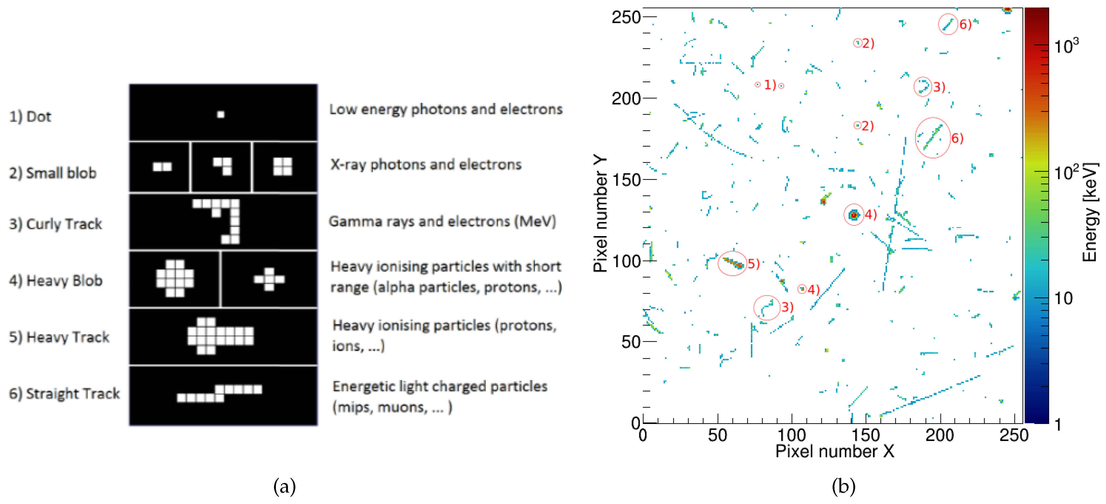
Figure 3.
Graphical visualisation of the response matrix () used for obtained through simulation.
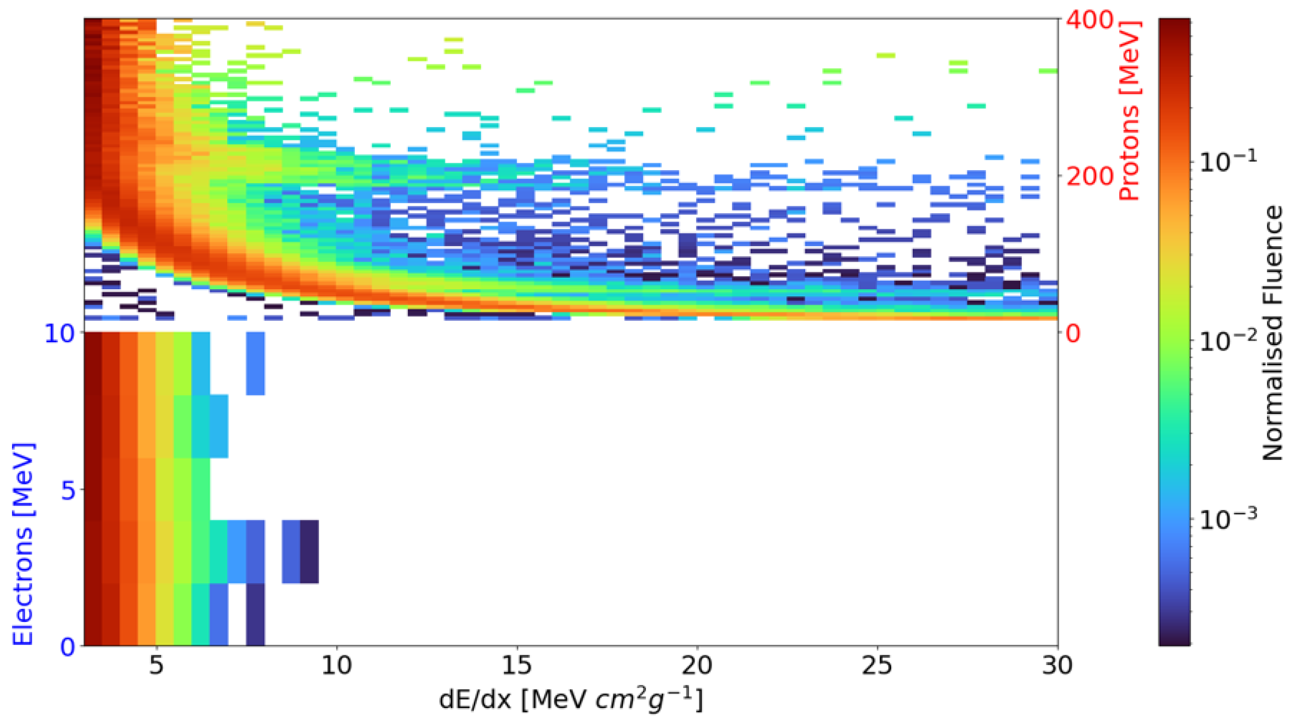
Figure 4.
3D reconstructions of tracks; (a) 120 GeV/c pion passing through a 500 µm thick silicon sensor; (b) high energy electron, (c) fragmentation reaction measured during exposure of a 2 mm thick CdTe sensor to a 180 GeV/c pion beam; (d) Cosmic muon with a 3D line fit. Fitting the trajectory allows a trajectory reconstruction with precision of µm evaluated at a distance of 1 m. From [29,30].
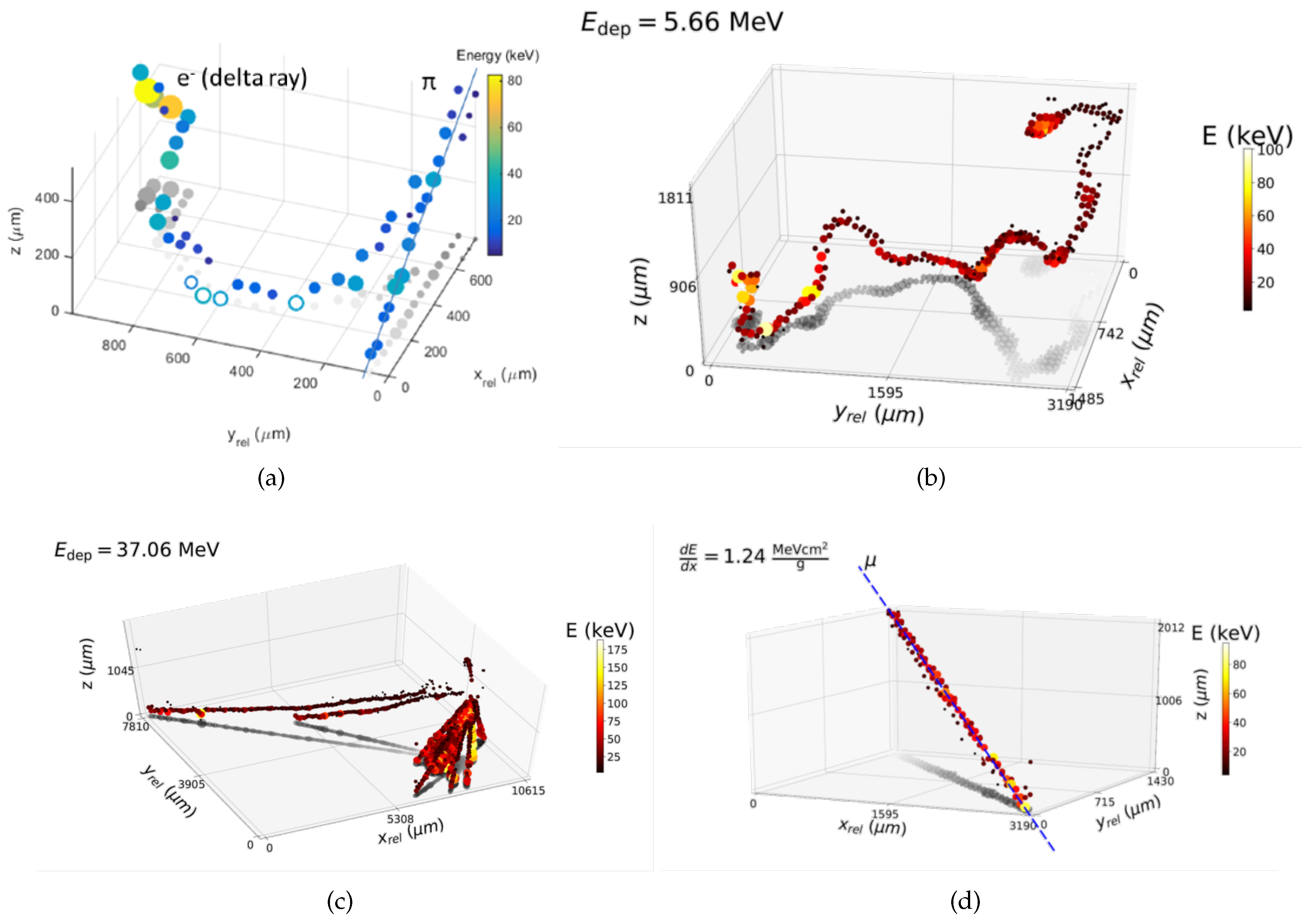
Figure 5.
Relative number of pixel classified as noisy on a weekly basis from August 2014 to the end of June 2023 for the Timepix in SATRAM. The number of noisy pixels stays below 0.6% until the end of 2021. In 2022, numbers are rising with a maximum of about 22% near the end of the year. The detector recovered in 2023.
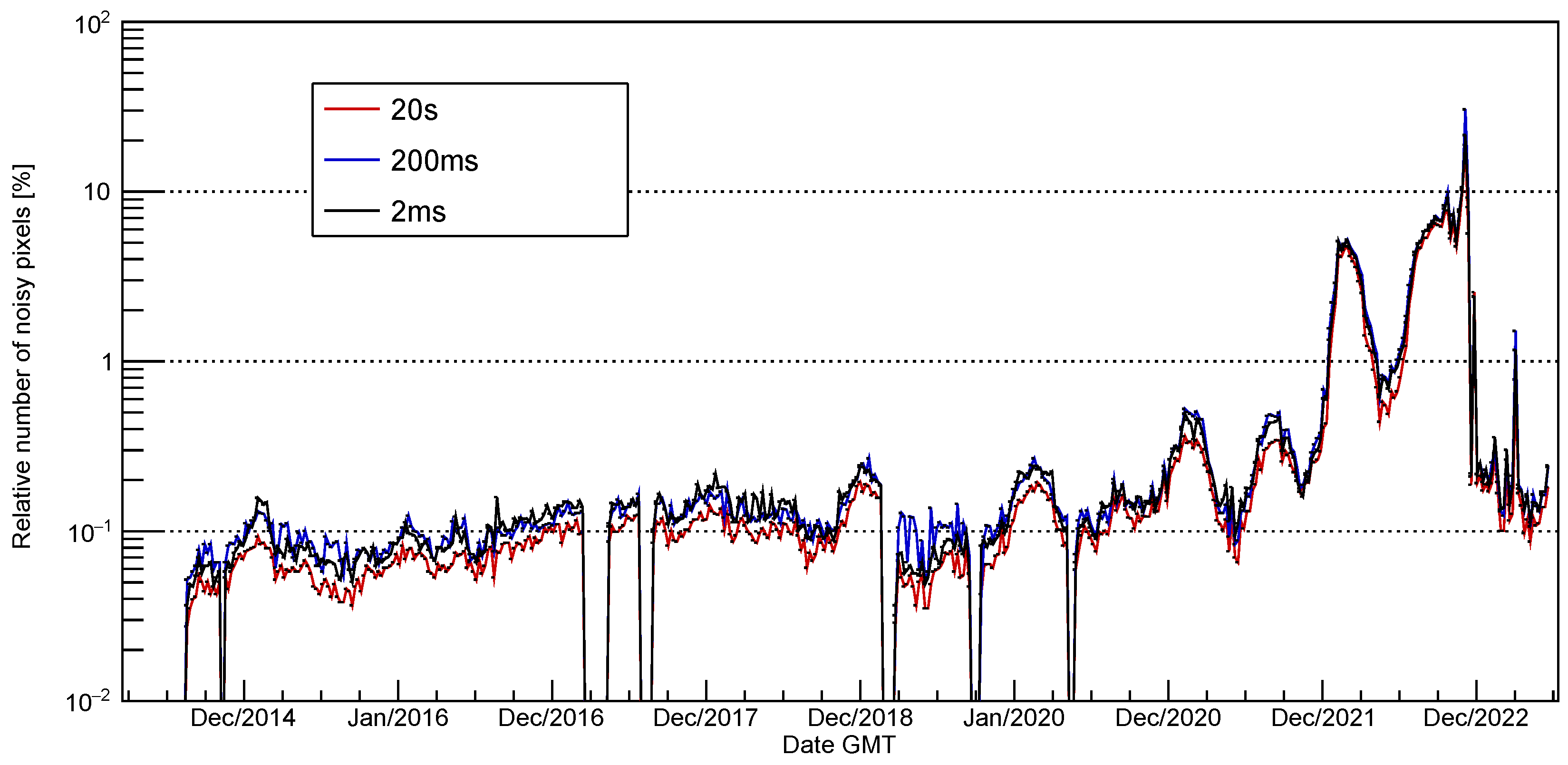
Figure 6.
Noisy pixel distribution over the Timepix sensor for the years (a) 2015 and (b) 2022. The pixels in the lower left corner got damage during launch of the Proba-V satellite. The color bar represents how often the pixels were considered noisy, on a weekly basis and across all three acquisition times.
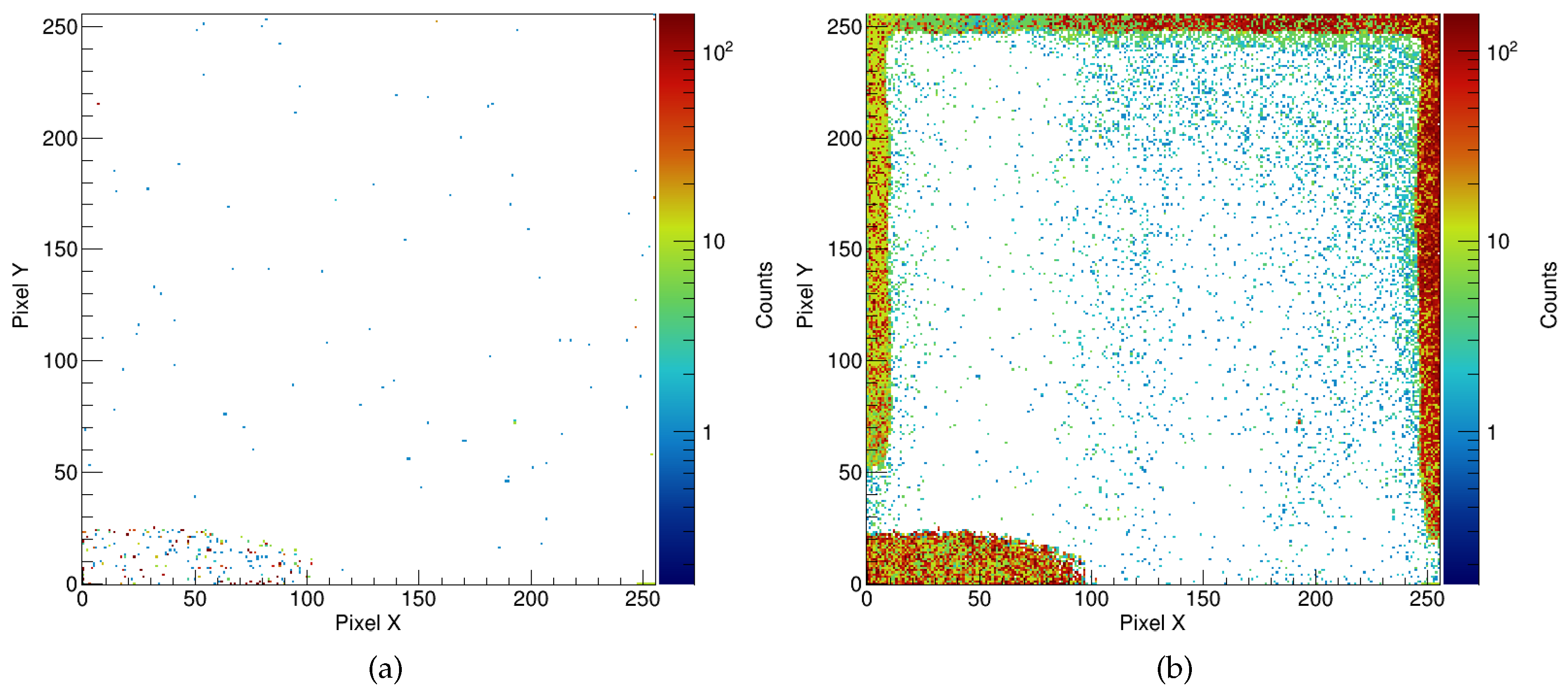
Figure 7.
Same as 5, but excluding noisy pixels from the lower left corner and pixels on the edges of the sensor as seen in 6(b). The number of noisy pixels is greatly reduced.
Figure 7.
Same as 5, but excluding noisy pixels from the lower left corner and pixels on the edges of the sensor as seen in 6(b). The number of noisy pixels is greatly reduced.
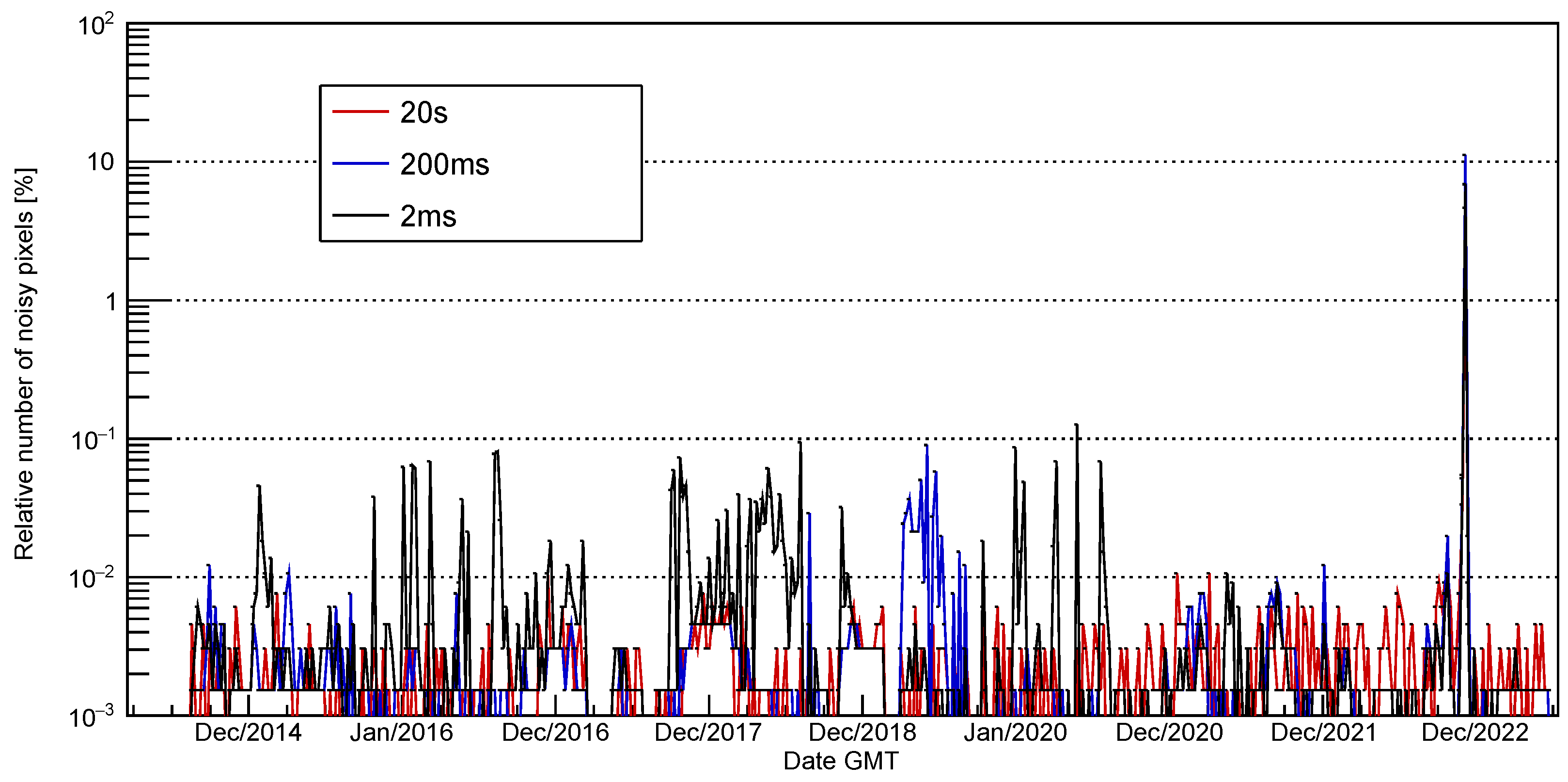
Figure 8.
Electron and proton flux rates as measured with SATRAM at 820 km altitude in low earth orbit, averaged over the years from 2015-2021.
Figure 8.
Electron and proton flux rates as measured with SATRAM at 820 km altitude in low earth orbit, averaged over the years from 2015-2021.
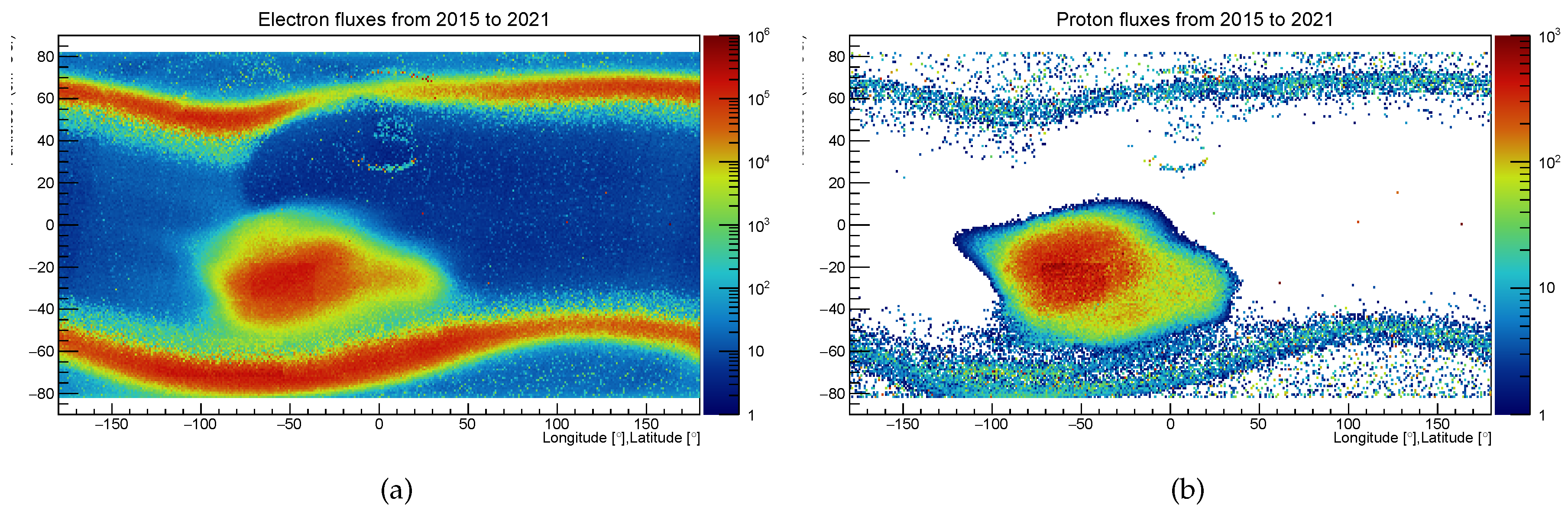
Figure 9.
(a) spectrum measured in the SAA used as input for the unfolding methodology; (b) Results of the unfolding methodology described in Sec. 2.4 to the spectrum of (a) (yellow line). The electron contribution determined in simulation (blue line, see text for details); (c) The final proton energy spectrum was determined by bin-wise subtraction of the yellow and blue curves of (b). The data was measured withing the SAA (longitude, latitute) at 820 km altitude with SATRAM.
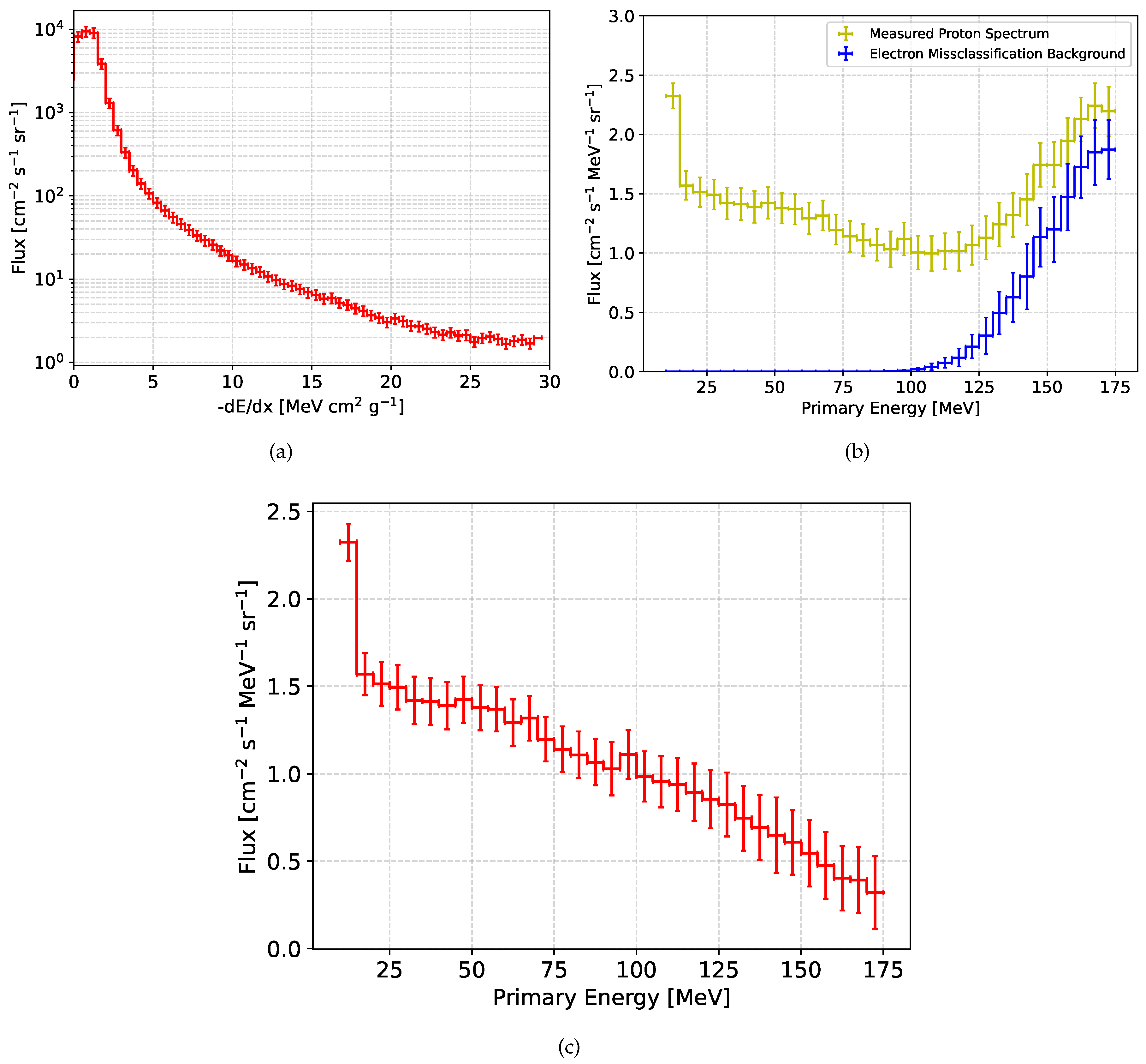
Figure 10.
(a) Picture of the Timepix3 2 × 2 module developed for the use in demonstrator of a penetrating particle analyzer; (b) Timepix3 quad integrated into the Mini.PAN front end.
Figure 10.
(a) Picture of the Timepix3 2 × 2 module developed for the use in demonstrator of a penetrating particle analyzer; (b) Timepix3 quad integrated into the Mini.PAN front end.
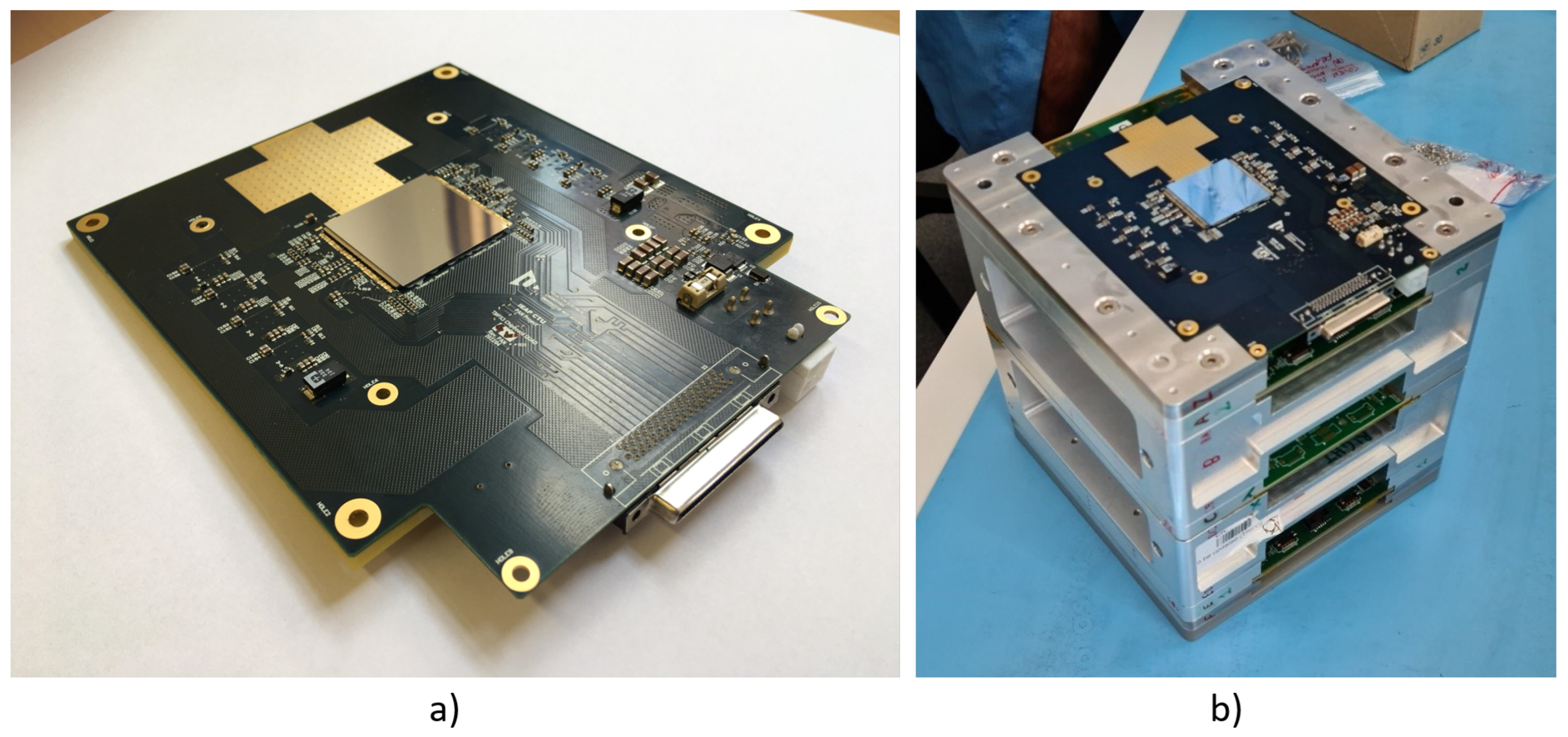
Figure 11.
Energy deposition spectra measured with the Timepix3 quad module in a 180 GeV/c pion beam fitted with a Landau curve convolved with a Gaussian: (a) at perpendicular particle impact; (b) at 30 degrees and (c) at 60 degrees impact angle with respect to the sensor normal.
Figure 11.
Energy deposition spectra measured with the Timepix3 quad module in a 180 GeV/c pion beam fitted with a Landau curve convolved with a Gaussian: (a) at perpendicular particle impact; (b) at 30 degrees and (c) at 60 degrees impact angle with respect to the sensor normal.
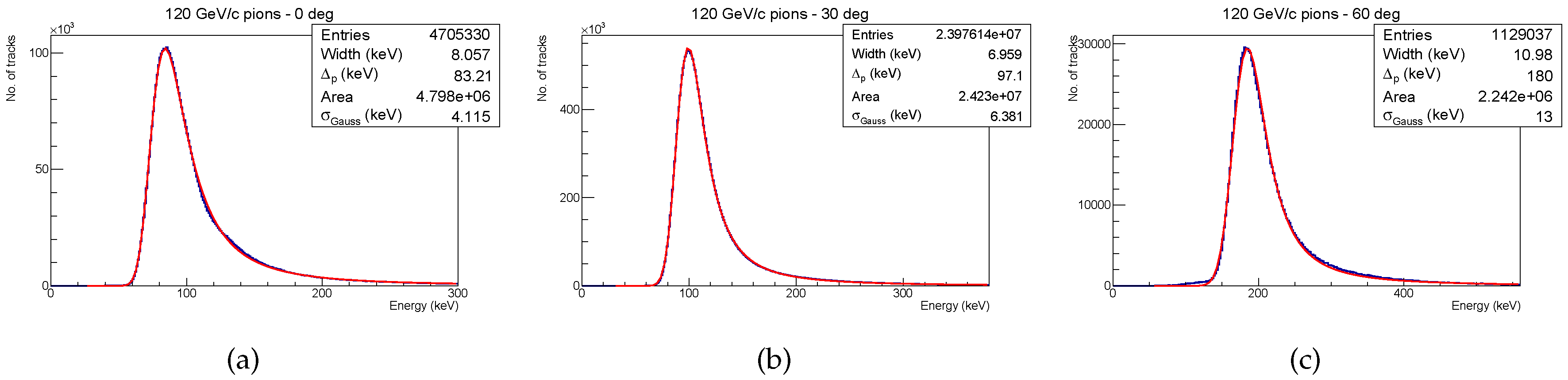
Figure 12.
(a) Experiment design; A collimated beam from a Hamamatsu microfocus X-ray tube hits a plastic target creating polarized X-rays which are absorbed in a 1 mm thick Timepix3 detector. The detector was placed at 90 to the axis defined by the tube and scattering target. A tube voltage kV was used at tube current = 60 A; (b) Energy histogram of the selected pairs of clusters. Compton scattering clusters with energies 3.5 keV could not be detected due to per pixel detection threshold.
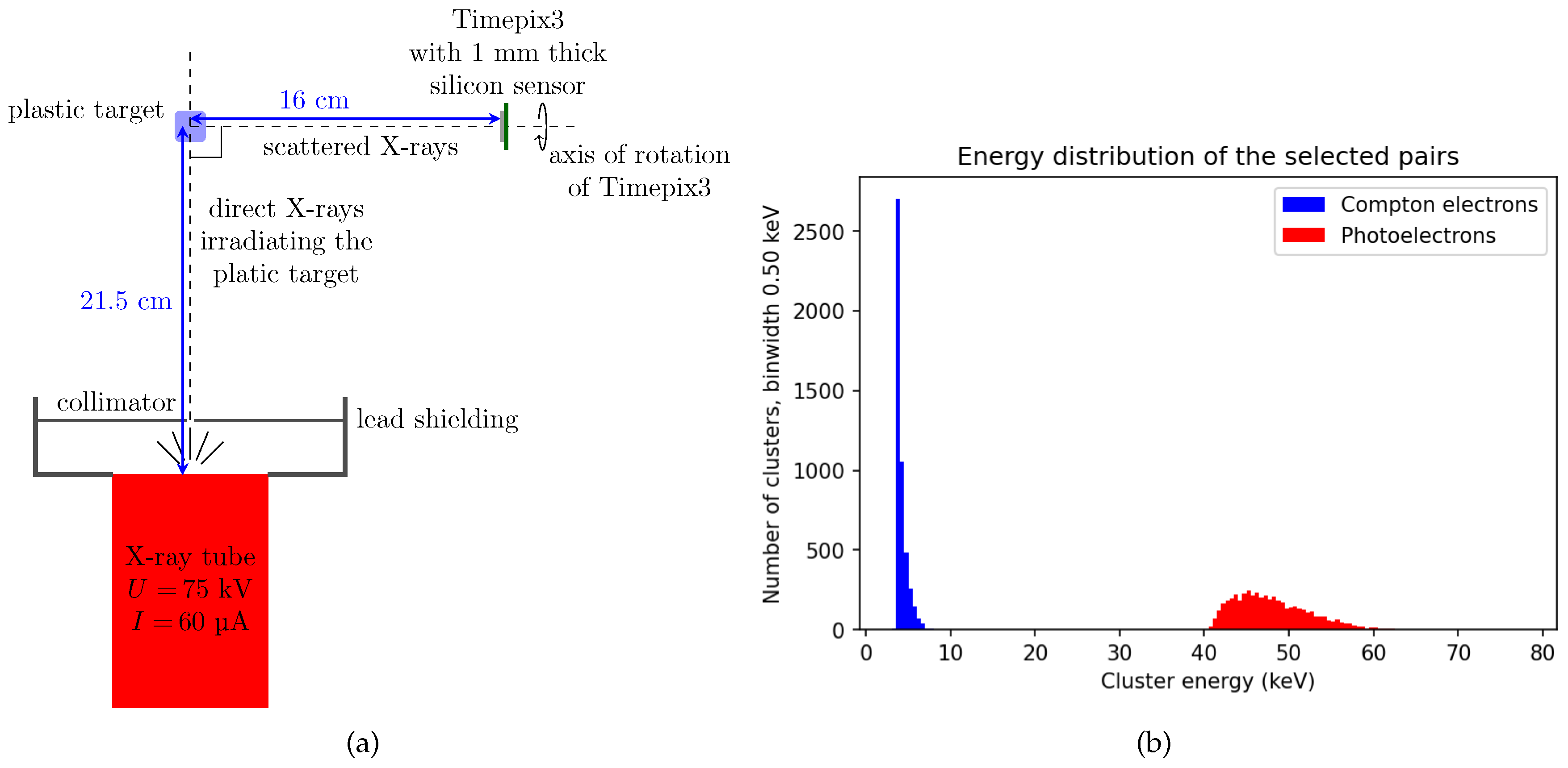
Figure 13.
Modulations measured within the detector plane presented at different angles around the axis defined by the target and detector.
Figure 13.
Modulations measured within the detector plane presented at different angles around the axis defined by the target and detector.

Figure 14.
Application of the single-layer Compton camera reconstruction to the measured data.
Disclaimer/Publisher’s Note: The statements, opinions and data contained in all publications are solely those of the individual author(s) and contributor(s) and not of MDPI and/or the editor(s). MDPI and/or the editor(s) disclaim responsibility for any injury to people or property resulting from any ideas, methods, instructions or products referred to in the content. |
© 2023 by the authors. Licensee MDPI, Basel, Switzerland. This article is an open access article distributed under the terms and conditions of the Creative Commons Attribution (CC BY) license (https://creativecommons.org/licenses/by/4.0/).
Copyright: This open access article is published under a Creative Commons CC BY 4.0 license, which permit the free download, distribution, and reuse, provided that the author and preprint are cited in any reuse.


