
Submitted:
15 November 2023
Posted:
16 November 2023
You are already at the latest version
Abstract
Acceleration rates of vehicles are crucially important statistics needed in two main aspects: first, they are essential to incident reconstructor professionals as having a verified database on where basing the cinematic reconstructions is definitely difficult and moreover, they are useful in order to understand how to create the safest possible environment on the road. This key topic gives es-sential information for road design like intersection schemes, acceleration and deceleration lane length as well as traffic simulation modelling and furthermore, to educate vehicle drivers when entering the traffic flow and to provide limit acceleration values needed to develop autonomous vehicle’s software in order to guarantee a comfort drive.
Literature reports tons of linear acceleration stats mainly referred to vehicle performances claimed by car manufacturers, but these data don’t recreate real drivers’ behaviour when entering the road by turning left or right or crossing an intersection. This work aims to integrate the most reliable data from literature with a hybrid and an electric vehicles statistic, adding also two contemporary thermal engine vehicles, extracted conducting probes that recreates real road environment.
The entirety of these experiments reconstructs the scenario in which a car is entering the traffic of a two-lanes road, from a stationary position at a stop sign and the acceleration rates are collected using a M.E.M.S. (Microelectromechanical system).
Finally, the space needed between the car that is about to enter or crossing the road and the car that is approaching the intersection is calculated, basing the computations on the acceleration values extracted from the probes. These spaces are pictured, as a way to give a concrete idea to readers.
Keywords:
Car Acceleration
; Traffic Accidents
; Road Design
; CAV Software Development
1. Introduction
The disposal of acceleration rates gathered from practical tests which recreate real road situations are fundamental to understand traffic modelling studies, road designing and autonomous vehicle’s software development.
The totality of these sectors of study refer to transport sustainability which is directly connected to road safety. Road crashes are a leading cause of death and serious injuries in both developed and developing countries and in particular, intersections are recognised as being among the most hazardous locations on the road. Nonetheless, all the research has the main aim to reduce road crashes in the most efficient way.
According to ISTAT [1] and ACI [2] statistics, in Italy during the year 2019, (just before the covid 19 pandemic) about people lost their lives and got injured in traffic. “Missed road precedence” was the second leading cause of accidents with of the overall, between “driving distractions” () and “speeding” . The social cost of the total amount of crashes consists to billions of Euros, that is about of the national GDP (Gross Domestic Product).
In detail, the traffic characteristics at an urban intersection are comprising slow- and fast-moving vehicles with considerable variation in vehicle features (such as vehicle size, weight and engine power) as reported from Mondal and Gupta [3] (p.2). Due to numerous such factors influencing vehicle acceleration and deceleration (A/D), a smaller number of studies are available in this area.
Academic works have examined A/D behaviour and found that A/D rates vary considerably from vehicle to vehicle depending on traffic, roadway, and environmental factors (Long [4]; Wang et al. [5]).
Reporting a very recent study, Mondal and Gupta [3] examined the A/D behaviour of various vehicles observed at a signal-controlled intersection. However, the previous study, as many others, only reports linear acceleration rates, while in this work the starting of vehicles is analysed when they are entering the traffic in the left going lane and in the right lane also, as it will be explained in detail along the dedicated chapter, and as it is examined in Murro [6] study. This academic work lastly cited, will be considered as a reference to this paper, while the step forward will be the conduction of the same tests with recent thermal, hybrid and electric powered cars.
As anticipated and reported in Berktaş and Tanyel [7] research, these data have a great importance, also in giving concrete values to delineate the behavioural characteristics of human drivers, as autonomous vehicles’ software are designed based on the assumptions made from field tests. Indeed, the software must be able to detect if the vehicle can complete the manoeuvres requested in a totally safe way. For example, when the autonomous car is at an intersection, the software, after detecting the speed of the other vehicles approaching the junction, is able to calculate how much time and space the vehicle has to avoid the collision. By supposing on these quantities, the car knows exactly the acceleration that the propulsion system will produce and knows if this acceleration value would still generate a comfort drive for the passenger, thanks to data collected from field studies. The results in this study, shows that autonomous vehicles produce the safest traffic scenario, because of their instantaneous reaction to external inputs and their decisions based on calculations, way more quickly and more reliable than human capacities. Then, it is analysed how under heavy traffic flow conditions, they may provide improvement in intersections’ capacity and performance, which represent a relevant characteristic in order to keep the transport sustainable.
Furthermore, the vast majority of papers (Snare [8]; Bokare and Maurya [9]; Choi and Kim [10]; Mondal and Gupta [3]) measured acceleration data deducted from digital tachograph applied algorithm, or GPS devices. In this study, accelerometer rates are empirically measured using a M.E.M.S. (Microelectromechanical system) capacitive accelerometer, which is known to be very precise.
Thanks to these stats, as anticipated, corners and intersections clearance time can be suggested, considering the distance covered by the vehicle and depending on drivers’ behaviour. The target is to implement precautionary measures in real road situations and, at the same time, to offer these types of acceleration rates to experts working in the incident reconstruction sector and working as autonomous vehicles’ software programmers, as they can dispose of an adequate literature selection.
1.1. Literary review
There are several studies related to vehicle acceleration behaviour and the rates empirically obtained by each of them are quite similar. In order to discretize the whole number domain of possible rates, previous studies have divided them into three distinct categories, according to drivers’ behaviours: slow start, average and quick start. This classification allows the authors to lower the number of tests to conduct and permits the comparison between results. In the past studies, the acceleration rate of a vehicle along a straight path is the most common, which can be considered for this study as the lengthwise cross of an intersection.
As a way to find an upper limit of the acceleration values, it is not considered reliable a value that is set to be higher than the one recorded using an average supercar in launch control start. This limit is the mean acceleration obtained considering a medium performance reported by sporty car manufacturers, in particular in . The value is calculated by considering the standard cinematic formula (1) and transforming the speed unit in so the delta becomes , then this value is divided for the time cited and lastly, an acceleration of is extracted. In resume, any acceleration will be considered reliable only if it’s lower than .
After an extensive review of the existent literature, it’s possible to notice common intervals related to quantities, for every type of start, as it is reported here.
In chronological order, Snare [8] found a max acceleration of , using a gasoline powered Saturn SL built in year 1995 with 126 horse power. Haas et al. [11] conducted research to determine driver deceleration and acceleration behaviour at stop sign-controlled intersections on rural highways without the impeding from other vehicles. The data was gathered during a 1996 Intelligent Cruise Control (ICC) Field Operational Test conducted in Michigan and reported an average acceleration value of which is equal to related to all final speeds. Furthermore, the authors declared that both deceleration and acceleration showed large variations about these average values and all the efforts done to explain these large variations in terms of several possible explanatory variables failed, attributing this to a stochastic phenomenon.
Murro [6] in his study, compared 35 different vehicles during his survey campaign, powered by various types of engines fuelled with gasoline, diesel, gas and hybrid. The tests conducted with each car consisted in starting still from a stop signal and entering the traffic flow towards left, right and crossing the intersection lengthwise.
The Figure 1 describes in the detail the measures of the paths in the intersection model used for the tests, compliant with the Italian average road length and width. Overall, 1080 valid experiments were conducted by different drivers. The medium acceleration rates found for every type of start are summarized in Table 1.
More recent studies like Bokare and Maurya [9] reported two different ranges referred to fuel class: maximum diesel car acceleration oscillates between 1.89 m/s2 and 2.23 m/s2 while gasoline powered cars go from to . Above data are obtained observing a large number of cars conducted by their owners in the traffic stream, on stretch of a two-lane Nagpur-Mumbai Highway in India.
Xu et al. [12] using a Buick GL8 found a maximum acceleration of . This quantity was registered using two different measurement systems, in order to double-check the values. These systems consist in a micromechanical sensor with a tri-axle accelerometer, which was placed inside the vehicle tested, while the second system consisted in an external measure of the speed with radar velocimeters activated by researchers placed along the longitudinal path.
The same year, Choi and Kim [10], over their research on fuel consumption and emissions when starting and driving a car, found a mean start acceleration value of and a max of 3.629 m/s2 measured with a digital tachograph, higher than the values written above. The researchers used a Hyundai Sonata produced in year 2009, powered by a 141 hp liquefied petroleum gas (LPG) engine. Huang et al. [13] in their study focused on Eco-driving technology, a research on the correlation between driver’s behaviour and emissions, adopted as critical aggressive acceleration the values of 2.598 m/s2for vehicle starting and during driving.
Moreover, under the same Indian traffic stream environment as Bokare and Maurya [9], Mondal and Gupta [3] reported that an average acceleration range set to be from to , extracted from GPS measures of car accelerations obtained under disordered traffic situations at a signalized intersection.
Considering that Table 1 from Murro [6] can legitimately resume all the acceleration rates cited above, in this study these values will be considered as the main reference because of the probes design affinity.
As in the previous papers, only vehicles from year 1990 to 2010 circa where utilized, in the new tests reported here the acceleration data are expected to be higher, adopting the same intersection layout, working with recent thermal powered vehicles and adding two contemporary hybrid and electric cars.
Concerning the acceleration profiles registered from the field experimentations, different A/D models were adopted along the years. As a global consideration, Glauz, Harwood, and John [14] proposed that the initial acceleration value is moderately low concerning the maximum acceleration value. It shows higher and lower values at lower and higher speeds, respectively. The A/D models proposed by many researchers based on prevailing traffic situations were mainly constant, two-phase acceleration model, linear A/D model, and polynomial (Samuels and Jarvis [15]; Rao and Madugula [16]; Akcelik and Biggs [17]; Bonneson [18]; Long [4]; Bham and Benekohal [19]). The constant A/D model is the simplest form, which assumes that the vehicle has a constant A/D rate throughout the traffic stream (Samuels and Jarvis [15]). Here, constant A/D model is adopted, considering that the aim is to extract average acceleration values measured when completing the manoeuvres, so knowing the exact acceleration value at a certain moment is not significant. Moreover, the maximum punctual acceleration values measured during the probes are way higher or even twice the average values reported at the conclusions.
Here is reported in Figure 2 an example of polynomial acceleration model for the sake of completeness, cited from Akçelik and Besley [20], where the values extracted are an average acceleration rate of and a maximum acceleration rate of .
However, the model that most of the researchers adopted is the linear-decreasing model because of its simplicity and accuracy. Briefly, the model focuses on the linear decrease of the acceleration value, registered when the speed increases in the motion. According to the model reported in Dabbour and Easa [21] (p. 3), the acceleration of a vehicle at any time, after starting from rest, is given by:
where:
a = dv/dt = α₋βv ± G₁∙g,
- a = acceleration rate (m/s²) corresponding to a certain speed v;
- v = vehicle speed (m/s);
- α = acceleration rate (m/s²) at the first instant of the period considered;
- β = rate of change of acceleration with respect to speed (s−1);
- G₁ = grade of minor road, positive if upgrade and negative if downgrade (m/m);
- g = gravity acceleration (9.80665 m/s²).
Concerning this model, the values reported as a result in every past study are α and β, which both assumes two different values in relation to the interval speed of the vehicle, in particular a first smaller quantity for the initial seconds (for example 5 seconds) when the measurement is started and the vehicle initiate the departure, and a bigger quantity when the car is in motion.
Dabbour [22] developed acceleration profiles based on actual drivers’ behaviour for light-duty vehicles starting from rest and turning to the right into roads with high traffic volumes. The values of α and β were and , respectively, during the first 5 s of departure, and and , respectively, afterward. For right turn departures into roads with moderate or low traffic volumes, the values of α and β were and −0.19284 s−1 respectively, during the first 4 s of departure, and 1.9854 m/s2 and , respectively afterward. Henceforward, α will be the only value reported from previous studies, as here considered as the most representative and the one that is more likely to be compared to an average acceleration value, bearing in mind that the outcome from the formula will result slightly lower in the second part because the second term is negative, and higher in the first part of the acceleration because the second term is positive.
The same type of research was conducted by Dabbour and Easa [23] but regarding the acceleration values by turning left in a two-lane road, which reported the two parameters of respectively while drivers where making the initial turning manoeuvre, and while drivers were accelerating along the major road after completing the initial turning manoeuvre. For a four-lane road the quantities are slightly different, in particular and as first and second value. Wang et al. [5] studied the acceleration behaviour of vehicles starting from rest at all-way stop-controlled intersections by collecting data from over 100 private vehicles in the Atlanta urban area that were equipped with GPS data logger devices. The model developed for straight departure found the value of α to be , while the α referred to turning departure was . In another study conducted by Dabbour et al. [24] on the minimum lengths of acceleration lanes based on actual driver behaviour and vehicle capabilities, revealed that the value of α when the entry ramp speed of the vehicle is included between is set to be .
Another sector of studies, already cited in the introduction chapter, where these values have been derived from field tests because of design necessity comprehend the research to set limit quantities of acceleration values for autonomous vehicles’ software. The most recent study on this topic has been conducted by Berktaş and Tanyel [7] where 15 volunteer drivers managed to obtain the values reported in the Figure 3, here below.
Moreover, upper and lower acceleration values for autonomous vehicles to keep the passengers in comfort situations are assumed to be and respectively.
One year before, Niels et al. [25] studied the impact of connected and autonomous vehicles on the capacity of signalized intersections in Münich. In their study, researchers focused not only on autonomous or connected vehicles but mixed traffic conditions that include human driven vehicles also. They assumed the maximum acceleration rate for autonomous vehicles as .
2. Materials and Methods
The measurement campaign has been conducted following a common protocol, disposed in order to guarantee homogenous conditions during the detections. The protocol is based on few main principles:
- Acceleration rates are measured using various cars;
- Testing sites are flat areas with asphalt floor in dry condition;
- Every vehicle was equipped with the same accelerometer that was calibrated before every acceleration probe;
- Every manoeuvre was repeated multiple times and all of them were executed guaranteeing the minimum path, reported in Figure 1.
2.1. Materials
The tools used throughout the study are the following:
- WitMotion© accelerometer sensor WT61C-TTL
- TTL cable + extension USB cable
- Laptop
- WitMotion software [26]
2.1.1. Accelerometer
As written above, the accelerometer sensor used is the WitMotion© WT61C, which is a high accuracy sensor that measures the acceleration in a range of with a resolution of and a frequency of . In noisy ambient or whenever is needed, there’s the possibility to set a static threshold related to the angle measures per second, that goes from the value of to as maximum. It is a M.E.M.S. (Microelectromechanical system) capacitive sensor, indeed it works by measuring the micro deformation of an elastic object where a face of the capacitor is placed. The other face is attached in front of the first one, but to a rigid part of the instrument. When the elastic material is elongated by the acceleration (which generates a force), the distance between the two faces of the capacitor increases or decreases, and the amount of this distance is calculated very accurately by the capacitive sensitivity of the circuit at which the sensor is connected. This instrument has also a Gyroscope with an accuracy of installed to measure the tilt angle. The sensor outputs the values after adjusting them with a built-in Kalman filter [27] which is an optimal filter for dynamic measurements and operates a first rough noise cancellation.
Figure 4.
(a) WitMotion© accelerometer sensor used during the tests, front and backview; (b) accelerometer fixed inside the Renault Zoe, connected to the laptop where the measurements were recorded.
Figure 4.
(a) WitMotion© accelerometer sensor used during the tests, front and backview; (b) accelerometer fixed inside the Renault Zoe, connected to the laptop where the measurements were recorded.
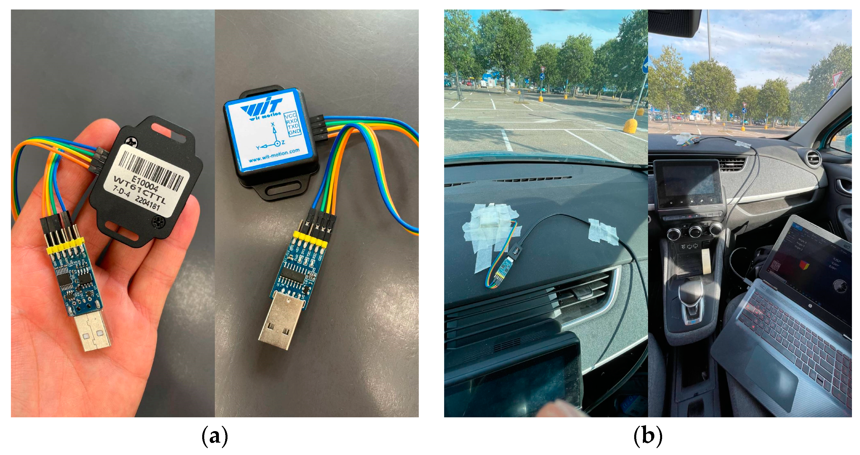
The sensor is opportunely attached to a plain surface of the vehicle interior to keep it motionless and integral with the car. Then it’s coupled to a laptop where the brand software was installed, in order to acquire and register data. The following image (Figure 5a) shows the software interface when the sensor is connected. The tilt angles are displayed in the “home screen” whether the accelerations are outputted at the voice “Data” near the top left corner of the window. In order, “Angle X” is related to the roll angle, “Angle Y” to pitch and “Angle Z” to yaw. By clicking the “Angle reference” key (top right corner) the sensor is calibrated to the position at which it is in that moment. This operation has been repeated at the starting of each acceleration probe because it may happen that during the test, the sensor could lose the reference.
The button “Record” (top left corner) stands in order to record the data registered during each probe; by clicking it, an interface window will appear (Figure 5b).
The software can record in different file formats. By ticking the “Mat” format box, the software registers the data into a MATLAB matrix. Here, after writing a simple code, it’s easy to obtain accurate graphs of each test, as shown in the next chapter.
2.2. Methods: In-situ simulations and vehicles used
The acceleration tests have been realized in two parking areas related to two commercial activities both closed during the experiments. These zones were chosen in relation to the need of finding sufficient big spaces, where recreate the same manoeuvres that are performed on the road at a real intersection. The areas were both clear from cars and people, and all the probes were conducted assuring that nobody was at risk.
The testing sites are flat areas with asphalt floor. The probes were conducted during summer sunny days and the ambient temperature was oscillating between and C (about 75÷90° F), while the temperature of the road was estimated to be around C (110÷140° F).
The vehicles used for the tests are two cars with thermal engine, one mild hybrid car and a full electric one, each one with a weight-to-power ratio included in 10÷20 kg/kW interval. In order:

Table 2.
Vehicles used for the tests.
| Car brand | Model | Engine type | Displacement [cc] | Power [kW] | Fuel type | Mass[kg] |
|---|---|---|---|---|---|---|
| Alfa Romeo | Stelvio | Thermal | 2143 | 154 | Diesel | 1745 |
| Fiat | 500X | Thermal | 1956 | 103 | Diesel | 1570 |
| Volvo | XC60 | Mild hybrid | 1969 | 145 | Diesel | 1892 |
| Renault | Zoe E-tech | Full electric | - | 80 | Electric | 1577 |
The first three cars were tested at the parking pictured in the Figure 6a, while the fourth car at the one in the Figure 6b.
As already mentioned, the accelerometer sensor was calibrated following every time the same procedure based on referring the three axes on the vehicle when it was stationary before starting the record and obviously before starting the acceleration. In detail, replicating the probes conducted in Murro [6] study, each test consisted in three manoeuvres:
- Lengthwise cross (LC);
- Left turn;
- Right turn.
Repeating every manoeuvre multiple times (at least five times), approaching them with three different drivers’ behaviour: Bulleted lists look like this:
- Slow start;
- Average start;
- Quick start.
All the probes were executed guaranteeing the minimum path, positioning in the parking zones some landmarks, identified by measuring the distances cited in Figure 1 from the starting point. These paths are designed in order to respect the medium Italian roadway width, expressly considered to be from to a maximum of , as cited on the Italian “Gazzetta Ufficiale” [28]. Respectively, the medium path travelled in each parking during the tests with the cars are depicted in the Figure 7.
The cars noted as “A” are the initial positions, while the note “B” indicates the finals. In detail, the measures taken as reference are the medium vertical distances from the starting to the final position of the vehicle in each path, set to be circa and respectively for the right and left turn, referred to the perpendicular position of the car “B”, while is used for the lengthwise cross distance.
2.3. Data analysis: MATLAB© code
The data from every acceleration test are instantaneously generated from WitMotion software [26] and outputted in different formats as previously exposed. In this paper, the MATLAB format is the only one considered, as all the stats will be then elaborated in a specific MATLAB program (prova.m). The functionalities developed in this code are fundamental in order to select the right data, sample, elaborate, calculate and graph all the values recorded and gathered by the accelerometer sensor and transcribed by the software in a matrix.
2.3.1. Input matrix
The matrix generated by the WitMotion software [26] in “.mat” format, containing all the values recorded by the sensor is made of columns and it comes with a legend that specify at which physical measure each column refers.
Figure 7.
Matrix legend.
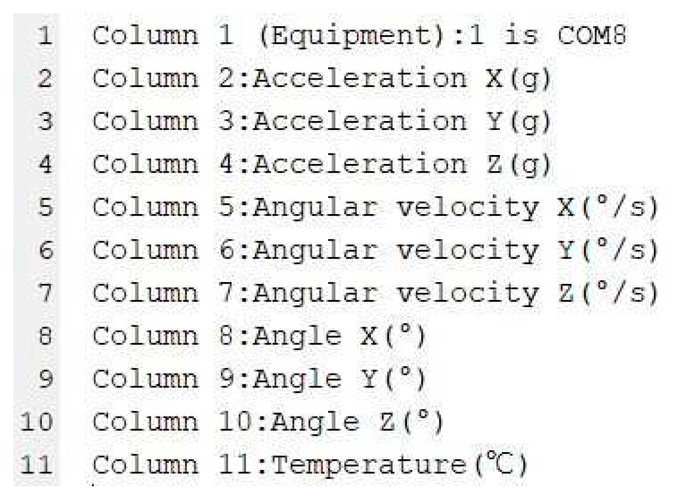
Column 1, as reported, refers to the USB port number of the laptop in which the accelerometer sensor is plugged via cable. Obviously, in order to guarantee the correct functionality of the sensor, this column must report the same number at every row. Then, from column number 2 to column number 10, the values reported are the planar accelerations along the three axes, the angular velocities and the angular accelerations, following the same order as listed. Last, the value of temperature is displayed but, considering that the sensor is placed on the car dashboard which is a black surface hit by the sun rays, this value may be overestimated and is not considered reliable.
The following image (Figure 8) is the display of the MATLAB matrix, referred to a randomly chosen test, screenshotted at random rows indexes.
As it was anticipated, column number one only displays the digit “1”. Noticing column number ten, only zeros are displayed because in that time lapse (), no pitch acceleration was detected.
The only variable missing is the time, which is reconstructed along the program code by knowing that each one of the eleven measures are outputted every hundredth of a second according to the frequency of the sensor, selected at .
After reading the input matrix, the program picks out the only values belonging to the column number 2, 3 and 4. The acceleration on the “X” axis is the most important value researched in these tests, while the other two acceleration measurements can be two useful indicators in ascertaining if a test can be reliable or not. The “Y” axis indicates the swerve intensity when left and right turn tests are conducted. If the acceleration reaches too high values, it means that the “X” acceleration measures will result distorted as they will be more correlated to human action than on vehicle response. Furthermore, the “Z” axis is a good indicator of a reliable test because the value that is displayed at the start of the record must be equal to gravity and, if the graph of this variable presents oscillations during the car motion, the amplitude of them can represent measurement disturbances.
In the following image (Figure 9), a plot of the three accelerations picked by the code is presented. It can be noticed that the values have been transformed from [g] unit to [m/s²] by multiplying them to gravity absolute value (). In particular, this graph refers to a fast linear acceleration, which was recorded when simulating the lengthwise cross of an intersection.
2.3.2. Noise filtering
Every sensor that measures dynamic variables is subject to noises and disturbances. As said in the previous chapters, the device used to record the data in this paper has a built-in Kalman filter, which works on an algorithm known as “linear quadratic estimation”, that uses a series of measurements observed over time, including statistical noise and other inaccuracies, and produces estimates of unknown variables that tend to be more accurate than those based on a single measurement alone, by estimating a joint probability distribution over the variables for each timeframe [27] (p. 1).
Even if the Kalman filter [27] is one of the most recommended for dynamic valuations, as it can be noticed in Figure 9, the high frequency value of measurements () at which the sensor is set, generates peaks in the graph, attributable to noises and errors. In order to smooth the plot, another mathematical algorithm is applied when programming the MATLAB code, which is the Savitzky-Golay [29] filter. It’s a digital filter that can be applied to a set of digital data points for the purpose of smoothing the data, that is, to increase the precision of the data without distorting the signal tendency. This is achieved, in a process known as convolution, by fitting successive sub-sets of adjacent data points with a low-degree polynomial by the method of linear least squares [29] (p. 1).
In order to recall this filter, MATLAB has a built-in function called “sgolayfilt” which can be adapted to the purposes of the user, as it is possible to choose the grade of the polynomial interpolation and the frame length. The result obtained in this paper is pictured here in Figure 10.
Comparing this graph to the one in Figure 9, as can be seen, the peaks that were synonym of noise are disappeared and the plotted lines are way smoother. This result is more likely proper to a car acceleration data.
2.3.3. Data sampling
Both in Figure 9 and Figure 10, the sensor starts to record before the beginning of the acceleration, when the car is still motionless and keep recording even after the path is travelled. Recording when the car is not moving would collect a lot of values near zero that will distort the medium evaluation by rounding down the result. Furthermore, it may happen that during the test, the driver would keep accelerating for a little while, even after the end of the path. This could lead to damage the precision of the data measured, as high values of acceleration would be counted from the sensor and they will raise up the medium acceleration value, reporting a digit that would be higher than the real one. For the purpose of possibly find the most accurate medium acceleration value, a precise data sampling method is indispensable.
To design the MATLAB sampling code, a meticulous interval in which taking count of the acceleration values measured must be set for every different type of test. As a way to outline this interval, the space travelled for each probe is taken as distinctive value. The paths are differentiated and stand to be for the lengthwise crossing, for the right turn and for the left turn, as pictured in Murro [6]. When running the code, the user will have to choose which path to consider according to the probe that has to be evaluated.
Designing the program, two main concepts are considered as a way to pick the right acceleration values belonging to the correct interval:
- A threshold of has been used to disregard all the measures recorded during the time when the car is motionless, as it has been considered that an acceleration under this rate does not affect the whole medium evaluation and/or would only represent noise.
- For the purpose of extracting the last meaningful acceleration value included in the space interval, the function that describes the progress of the “x” interpolation (Figure 10) has been integrated twice, finding the speed function and the space travelled.
Here, starting from knowing the last discrete digit belonged to the maximum space travelled inside the path, the program extracts its corresponding index which reveals to be the last consistent time value to consider, in order to sample the acceleration plot. Thanks to this procedure, a vector containing the exclusive acceleration measures included in the path is created and can be easily plotted, as reported here below in Figure 11.
3. Results
3.1. Average acceleration rates and interpretation
At the end of the described MATLAB code, the program is able to calculate the medium acceleration values solely considering the measures inside the interval referred to the paths. In fact, the statistic results of these sampled acceleration tests are simply the arithmetic mean, as it has been assessed as an effective way to resume the values measured in every instant of time, and a successful outcome to be used by the incident reconstruction professionals in figuring out the exact cinematic of the event, which is the main purpose of this work.
The code has been run for every probe conduced with all the four vehicles considered, elaborating a medium acceleration result for each one of the three driver behaviours. Subsequently, the totality of the outcomes has been gathered inside an EXCEL [30] table, dividing them by the different types of tests, as shown below (Figure 12).
Giving consideration to Figure 12, the “medium” and “±” rows have been created to report, respectively, all the arithmetic means of the values measured in the same column and the average absolute deviation of the values from their means. The first one is useful in resuming all the outcomes from the probes while the second one clarifies how much the results changed from each test to the next, in order to highlight the reliability of every mean. In fact, keeping in mind that all the tests are conducted each time under the same conditions, if the results are comparable, or differ for a little quantity, it means that the average value represent them very accurately. On the other hand, if the deviations are big values and so the results differ too much, the average value it’s just indicative and the real measure caught on the test could vary a lot.
The last row (“between cars”) of every sub-table collects and reports the average values calculated from the means of each vehicle, catalogued for the three distinct driver behaviours, with the average of the absolute deviations determined from the pre-calculated mediums.
As a way to understand how much the average deviation can impact the time that a car takes to cross lengthwise an intersection, starting motionless, hereby two different acceleration values took as an example, chosen as the extremes of the deviation range of from reference, are considered:
- Mean acc. ;
- Mean acc. .
With the aim of calculating the time took by the car to complete the crossing, two physics formulas are observed, both taken from uniformly accelerated motion considerations:
the first equation (equation 2) is used to quantify the speed term at the end of the path, chosen as a straight line of . The acceleration terms chosen are previously described.
v² = v₀² + 2∙a(s-s₀),
Considering that in both cases, v₀ = and (s-s₀) = , the results are reported: added as follows:
- v₁ = √ (2∙2∙7) = ;
- v₂ = √ (2∙3∙7) = .
Now that the speed at the last moment of the car inside the path is known, the total ∆v is clear and it is possible to estimate the time took by the car to complete the manoeuvre in both hypotheses. To do so, the mean acceleration formula, here reported, is used:
v = v0 + a·t,
Considering the inverse formula, time will result:
- t₁ = v₁/a₁ = 5,3÷2 = ;
- t₂ = v₂/a₂ =6,5÷3 = .
Finally, the time difference between the cases is quantified as which is starting to assume a significant value. Therefore, the average deviation of will be taken as the threshold in the evaluation of a mean acceleration reliability. Noticing that the biggest deviation value reported in Figure 12 is , the totality of the measures presented can be considered reliable and notable.
4. Discussion
The last function written in the MATLAB code is developed to understand when the driver of the car that wants to cross the intersection or enter in the traffic flow, is able to complete the manoeuvre in complete safety. Indeed, the purpose is to make the drivers aware of the described situations, by calculating and visualizing the space necessary between the vehicles involved.
In detail, the program determines the interval of time that the car needs to cross the intersection by using the equation 2 and the equation 3, considering the case of fast accelerations and adopting the average quantities reported in Figure 12, for every type of manoeuvre. The “delta” space used in equation 2, is the sum of the path correlated with the manoeuvre considered, plus the length of an average car, took as . Taking into account that the program can only refers to a real measured probe, the values of acceleration adopted in the two equations are the closest to the ones calculated, thoroughly for lengthwise crossing instead of , for right turning instead of and finally instead of for left turning. The values chosen are respectively picked from the test conducted with the vehicle “Fiat 500X”, from the again conducted with the “Fiat 500X” and lastly from the probe conducted with the “Alfa Romeo Stelvio”.
The results of the minimum distances calculated are reported in the Table 3. Keeping in mind that these outcomes are correlated with a constant speed kept by the car incoming to the intersection, the values in terms of spaces are considerable. The first three speeds are selected considering the average speed limits existing in Italy, nearby junctions in both urban and extra-urban roads, while the “” speed is reported for the sake of completeness. here:
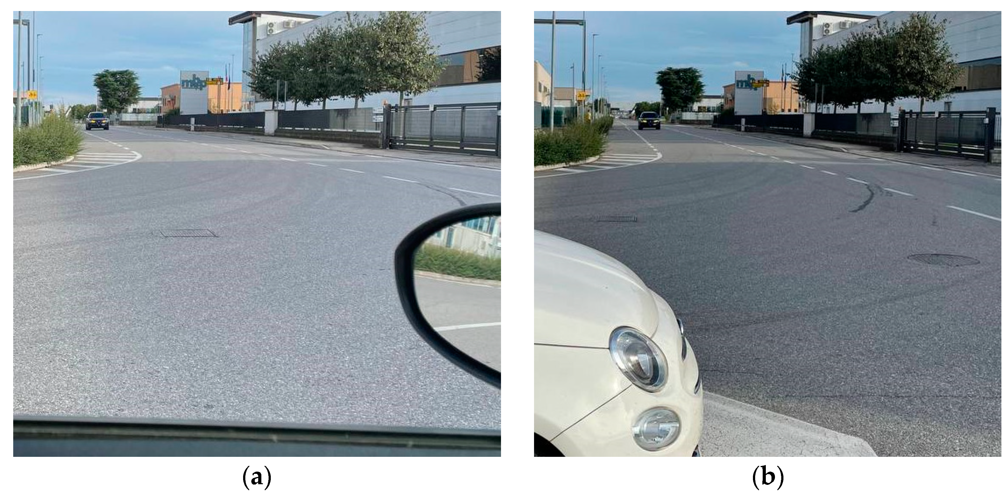
In order to have a concrete idea of the quantities assessed, different images are depicted here and visualize in terms of space the distances between the car standing at the stop signal and the vehicle incoming when the gaps are , , and meters. Left pictures are shot from the driver’s point of view, while the right ones from a wider perspective.
Figure 13.
Photo related to the vehicle incoming at 10 meters distance: (a) Driver’s point of view; (b) Intersection perspective.
Figure 13.
Photo related to the vehicle incoming at 10 meters distance: (a) Driver’s point of view; (b) Intersection perspective.
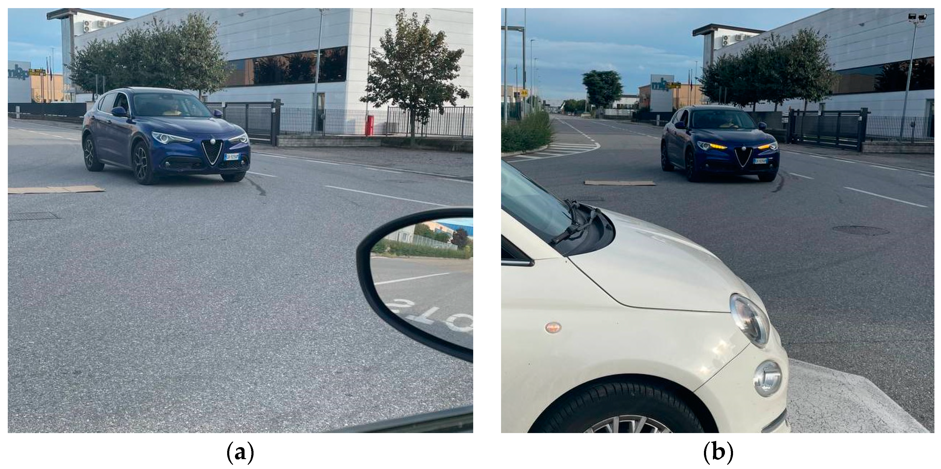
Figure 14.
Photo related to the vehicle incoming at 30 meters distance: (a) Driver’s point of view; (b) Intersection perspective.
Figure 14.
Photo related to the vehicle incoming at 30 meters distance: (a) Driver’s point of view; (b) Intersection perspective.
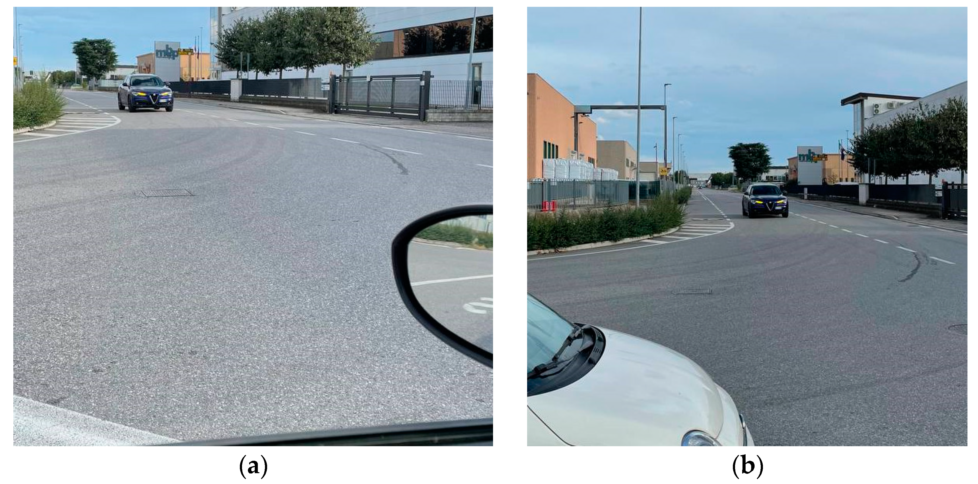
Figure 15.
Photo related to the vehicle incoming at 50 meters distance: (a) Driver’s point of view; (b) Intersection perspective.
Figure 15.
Photo related to the vehicle incoming at 50 meters distance: (a) Driver’s point of view; (b) Intersection perspective.

Figure 16.
Photo related to the vehicle incoming at 70 meters distance: (a) Driver’s point of view; (b) Intersection perspective.
Figure 16.
Photo related to the vehicle incoming at 70 meters distance: (a) Driver’s point of view; (b) Intersection perspective.
Considering the pictures above, the interspaces between the two vehicles used for the photos are detected with a professional laser sensor (specifically the “Leica® Disto D2”) and so they can be considered accurate.
The driver can notice how far the incoming vehicle appears to be, keeping in mind that the distances calculated in Table 3 reports the minimum spaces needed to complete the manoeuvres in safety conditions. Furthermore, these values are even higher than the spaces depicted in the images, especially focalizing on the left turn, which is the manoeuvre that takes the biggest path length ().
These results have the purpose to raise awareness among drivers, on the crossing operations when in proximity of an intersection. Noticing the large distance gaps needed between the involved cars, it is recommended to be extremely cautious in order to reduce the number of traffic accidents, as usually the spaces are underestimated, while the driver abilities are overrated.
5. Conclusions
5.1. Resume
The main purpose of this study is to obtain accurate car acceleration values from a still start at a stop sign when crossing an intersection or entering in the traffic flow, which are useful and precious for the professional workers in the incident reconstruction sector, for intersection design and for CAVs software development. These values have been acquired by conducting a measuring campaign of 197 probes with 4 different vehicles, calculating and resuming the average means. The types of tests have been divided into three categories related to the kind of manoeuvre realized, which are in turn, subdivided into three distinct driver’s approach.
The data has been obtained using an accelerometer sensor placed onboard, connected and monitored by a laptop that run its software and recorded all the measures. Then, the records have been elaborated, sampled and pictured thanks to a MATLAB code programmed by the author, which gave the results that has been collected in an EXCEL file.
Before reporting the results achieved, in order to describe the applicability conditions, it’s important to recall that:
- The number of probes sustained has been equally distributed between the manoeuvres of lengthwise crossing, left turn and right turn, executed adopting fast, average and slow starts;
- The totality of tests has been conducted in flat surface sites, pictured in Figure 6, with asphalt pavement, in dry conditions and hot weather. The cars were driven by the author of this study, who is a 26-year-old male with 8 years of driving experience;
- The four cars (illustrated in Table 2) used for the tests present a weight-to-power ratio included in interval, two of them powered by a Diesel engine, one with a mild-hybrid Diesel powertrain and the last one fully electric;
- The accelerometer is a highly accurate capacitive sensor as described more in detail in paragraph 2.1.1, which was opportunely attached to a plain surface of each vehicles interior and was calibrated every time before the start of each probe;
- The values deducted in this work are sampled and then calculated following the arithmetic mean and the average deviation of each value from the mean.
Finally, the results reported from the experiments and gathered in the Figure 12, are displayed here:
Table 4.
Resumed acceleration tests results.
| Unit [m/s²] | Quick start | Average start | Slow start |
|---|---|---|---|
| Lengthwise crossing | 2,91 ÷ 3,35 | 1,49 ÷ 2,33 | 0,71 ÷ 1,31 |
| Right turn | 1,68 ÷ 2,00 | 1,09 ÷ 1,41 | 0,65 ÷ 1,03 |
| Left turn | 1,70 ÷ 2,46 | 1,10 ÷ 1,64 | 0,75 ÷ 1,07 |
Additionally, in order to raise awareness among car drivers, the estimate time that each of the manoeuvres take has been calculated to get to the ultimate aim, which is finding how much space a car that is about to cross the intersection (or entering the traffic) in a safe method needs from a car that is approaching to the junction. The calculations (Figure 13) are reported considering the vehicle travelling to the intersection at four different constant speed, adopting 5 m as the length of the car that is about to cross. Figure 13, Figure 14, Figure 15 and Figure 16 are extracted from photos taken at road experiments and helps to have a concrete idea of the measures of space calculated.
5.2. Final considerations
By the evaluation of the outcome digits obtained in this study, some considerations can be elaborated:
- Broadly, the average values achieved from the tests set to be the lowest for the right turn manoeuvre and the highest for the lengthwise crossing. This phenomenon might be explained considering the human action as a deterrent to reach high acceleration values, because the combinations of accelerating and steering in turning to a narrow curve leads to more energy dispersion than the sole action of accelerating in a straight direction. As a matter of fact, circular motion acceleration is the product of a centripetal and a tangential vector, where only the last one increases or decreases speed while the centripetal is necessary to keep a circular path and it transforms into friction between the tyres and the asphalt, which generates energy losses;
- Along the study, the influence of the weight-to-power ratio on the acceleration results is not discussed. On this topic, Murro [6] reported that after conducting a statistic analysis, this ratio doesn’t considerably affect the estimation of the values, but it has a minimum impact on the dispersion interval width calculated from the average mean values. Reporting the conclusion on this discussion, the vehicles with lower weight-to-power ratio present a more uncertainty traduced in a wider deviation from the reference value, while the vehicles with higher ratio present a smaller deviation;
- The influence of driver’s age on the test measures is not analysed, but in any case, the predecessors’ studies didn’t find any correlation even though the drivers with less experience used to have a more cautious behaviour;
- Comparing the results found in this study (Table 4) with those reported from precedent papers and cited inside the literary review, the values are comparable with Murro [6] reports while they are higher related to all the other citations. This contrast might be caused by the different instruments used in measuring the acceleration values (GPS instead of MMS sensor), different layout scheme of the probes and dissimilar purpose of the test, while on the other hand, lots of analogies with Murro [6] in planning the probes and the type of sensor adopted (chosen to keep a continuity in the study reason), led to similar values, even if the cars used in these probes and the instruments are much recent;
- Bearing in mind the calculations of the space needed between the cars reported in Table 3, it is important to specify that the time considered when computing these measures is the sole interval that goes from the moment in which the tyres move on the asphalt to the moment in which the last protruding part of the car completes the path selected. In reality, when a car driver decides to perform the manoeuvre, many time frames elapse between the decision and the actual moment in which the car starts to move. For example, the psychotechnical interval of the driver, or the actual response of the actuators and the control unit of the vehicle, or the technical time required for the engine to deliver power at the tyres. All of these variables are taken into account in detailed incident reconstructions and add space to the outcomes found during this study, that are based only on the completion of the manoeuvres. Therefore, even though the pictures at Figure 13, Figure 14, Figure 15 and Figure 16 delineate a space that seems to be wider than the reality, it must be even more enlarged. As a matter of fact, the highest level of prudence is always required on the road, to prevent every sort of incidents.
Finally, what has been reported along this study cannot be considered as a point of arrival, but rather be a working basis to further developments and analyses. Furthermore, it is here proposed to conduct additional measurements in the future, with the concept of broaden the statistical basis, for example by comparing results obtained with different types of road surface and in dissimilar road surface conditions, or in relation of a bigger number of drivers of different ages and different sex, or also conducting the probes with a wider range of vehicles powered by the totality of fuel types currently on the market.
Funding
This research received no external funding.
Conflicts of Interest
The authors declare no conflict of interest.
References
- ISTAT Infografica sugli incidenti stradali - Anno 2019. Available online: https://www.istat.it/it/archivio/245759 (accessed on 9 November 2023).
- ACI Gli incidenti stradali 2019 nelle 106 province italiane. Available online: http://www.aci.it/archivio-notizie/notizia.html?cHash=e00a4d4f57218391bf026cd673232436&tx_ttnews%5Btt_news%5D=2378 (accessed on 9 November 2023).
- Mondal, S.; Gupta, A. Evaluation of Driver Acceleration/Deceleration Behavior at Signalized Intersections Using Vehicle Trajectory Data. Transportation Letters 2023, 15, 350–362. [Google Scholar] [CrossRef]
- Long, G. Acceleration Characteristics of Starting Vehicles. Transportation Research Record 2000, 1737, 58–70. [Google Scholar] [CrossRef]
- Wang, J.; Dixon, K.K.; Li, H.; Ogle, J. Normal Acceleration Behavior of Passenger Vehicles Starting from Rest at All-Way Stop-Controlled Intersections. Transportation Research Record 2004, 1883, 158–166. [Google Scholar] [CrossRef]
- Murro, A. Valori accelerometrici dei veicoli in immissione nelle intersezioni. ASAIS: Associazione per lo Studio e l’Analisi degli Incidenti Stradali, 2009; 1–48. [Google Scholar]
- Şentürk Berktaş, E.; Tanyel, S. Effect of Autonomous Vehicles on Performance of Signalized Intersections. J. Transp. Eng., Part A: Systems 2020, 146, 04019061. [Google Scholar] [CrossRef]
- Snare, M.C. Dynamics Model for Predicting Maximum and Typical Acceleration Rates of Passenger Vehicles, Virginia Polytechnic Institute and State University: Blacksburg, Virginia, 2002.
- Bokare, P.S.; Maurya, A.K. Acceleration-Deceleration Behaviour of Various Vehicle Types. Transportation Research Procedia 2017, 25, 4733–4749. [Google Scholar] [CrossRef]
- Choi, E.; Kim, E. Critical Aggressive Acceleration Values and Models for Fuel Consumption When Starting and Driving a Passenger Car Running on LPG. International Journal of Sustainable Transportation 2017, 11, 395–405. [Google Scholar] [CrossRef]
- Haas, R.; Inman, V.; Dixson, A.; Warren, D. Use of Intelligent Transportation System Data to Determine Driver Deceleration and Acceleration Behavior. Transportation Research Record 2004, 1899, 3–10. [Google Scholar] [CrossRef]
- Xu, J.; Lin, W.; Wang, X.; Shao, Y.-M. Acceleration and Deceleration Calibration of Operating Speed Prediction Models for Two-Lane Mountain Highways. J. Transp. Eng., Part A: Systems 2017, 143, 04017024. [Google Scholar] [CrossRef]
- Huang, Y.; Ng, E.C.Y.; Zhou, J.L.; Surawski, N.C.; Chan, E.F.C.; Hong, G. Eco-Driving Technology for Sustainable Road Transport: A Review. Renewable and Sustainable Energy Reviews 2018, 93, 596–609. [Google Scholar] [CrossRef]
- Glauz, W.D.; Harwood, D.; John, A.D.S. Projected Vehicle Characteristics through 1995. Transportation Research Record 1980, Journal of the Transportation Research Board 772, 37–44. [Google Scholar]
- Samuels, S.; Jarvis, J. Acceleration and Deceleration of Modern Vehicles. Australian Road Research Board 1978, 86, 23–29. [Google Scholar]
- Rao, S.K.; Madugula, M. Acceleration characteristics of automobiles in the determination of sight distance at stop-controlled intersections. Civil engineering for practicing and design engineers 1986, 5, 487–498. [Google Scholar]
- Akçelik, R.; Biggs, D.C. Acceleration Profile Models for Vehicles in Road Traffic. Transportation Science 1987, 21, 36–54. [Google Scholar] [CrossRef]
- Bonneson, J.A. Modeling Queued Driver Behavior at Signalized Junctions. Transportation Research Record 1992, 99–107. [Google Scholar]
- Bham, G.H.; Benekohal, R.F. Development, Evaluation, and Comparison of Acceleration Models. In Proceedings of the 81st Annual Meeting of the Transportation Research Board, Washington, DC; Washington, DC, 2002; Vol. 6. [Google Scholar]
- Akçelik, R.; Besley, M. Acceleration and Deceleration Models. 23rd Conference of Australian Institutes of Transport Research 2002, 1–10. [Google Scholar]
- Dabbour, E.; Easa, S.M. Revised Method for Calculating Departure Sight Distance at Two-Way Stop-Controlled (TWSC) Intersections. Transportation Research Record 2021, 2675, 904–914. [Google Scholar] [CrossRef]
- Dabbour, E. Design Gap Acceptance for Right-Turning Vehicles Based on Vehicle Acceleration Capabilities. Transportation Research Record 2015, 2521, 12–21. [Google Scholar] [CrossRef]
- Dabbour, E.; Easa, S. Sight-Distance Requirements for Left-Turning Vehicles at Two-Way Stop-Controlled Intersections. Journal of Transportation Engineering, Part A: Systems 2016, 143. [Google Scholar] [CrossRef]
- Dabbour, E.; Easa, S.M.; Dabbour, O. Minimum Lengths of Acceleration Lanes Based on Actual Driver Behavior and Vehicle Capabilities. J. Transp. Eng., Part A: Systems 2021, 147, 04020162. [Google Scholar] [CrossRef]
- Niels, T.; Erciyas, M.; Bogenberger, K. Impact of Connected and Autonomous Vehicles on the Capacity of Signalized Intersections – Microsimulation of an Intersection in Munich. Proceedings of 7th Transport Research Arena TRA 2018 2018, 1–10. [Google Scholar]
- WitMotion Shenzhen Co., Ltd. WitMotion Software.
- Kalman Filter. Wikipedia 2023.
- Gazzetta Ufficiale Art.1: Regolamento per l’esecuzione Del Testo Unico Delle Norme Sulla Disciplina Della Circolazione Stradale . Available online: https://www.gazzettaufficiale.it/atto/serie_generale/caricaArticolo?art.versione=1&art.idGruppo=1&art.flagTipoArticolo=1&art.codiceRedazionale=059U0420&art.idArticolo=1&art.idSottoArticolo=1&art.idSottoArticolo1=10&art.dataPubblicazioneGazzetta=1959-06-30&art.progressivo=0 (accessed on 9 November 2023).
- Savitzky–Golay Filter. Wikipedia 2023.
- Microsoft Corporation Microsoft Excel 2018.
Figure 1.
Intersection and probes layout adopted for the field tests.

Figure 2.
Example of acceleration plot in polynomial model.
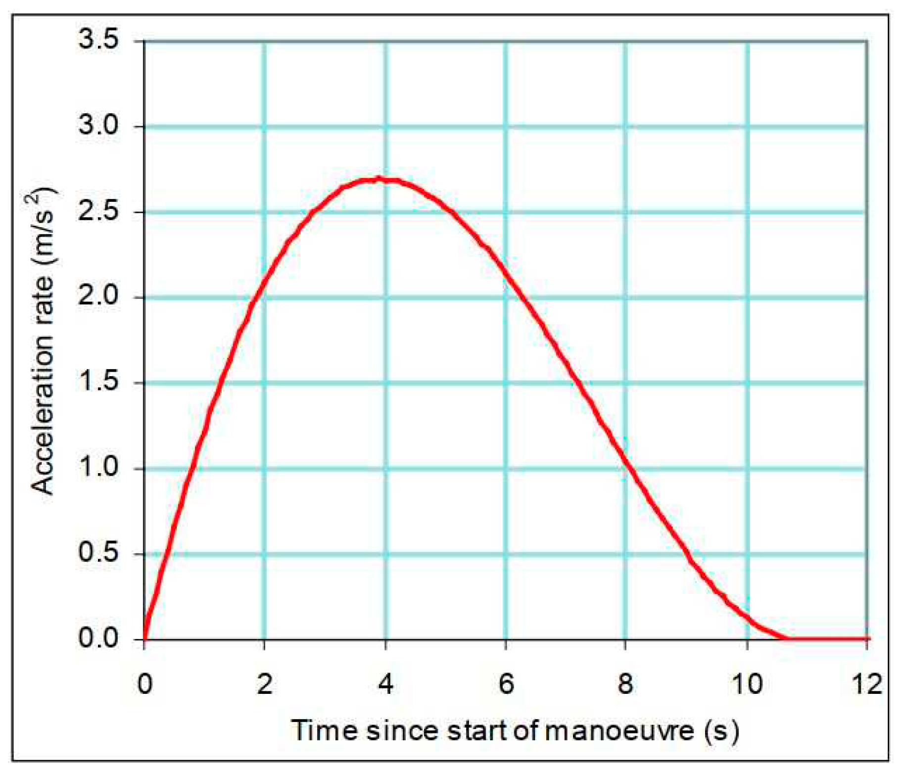
Figure 3.
acceleration values reported in Berktaş and Tanyel study.
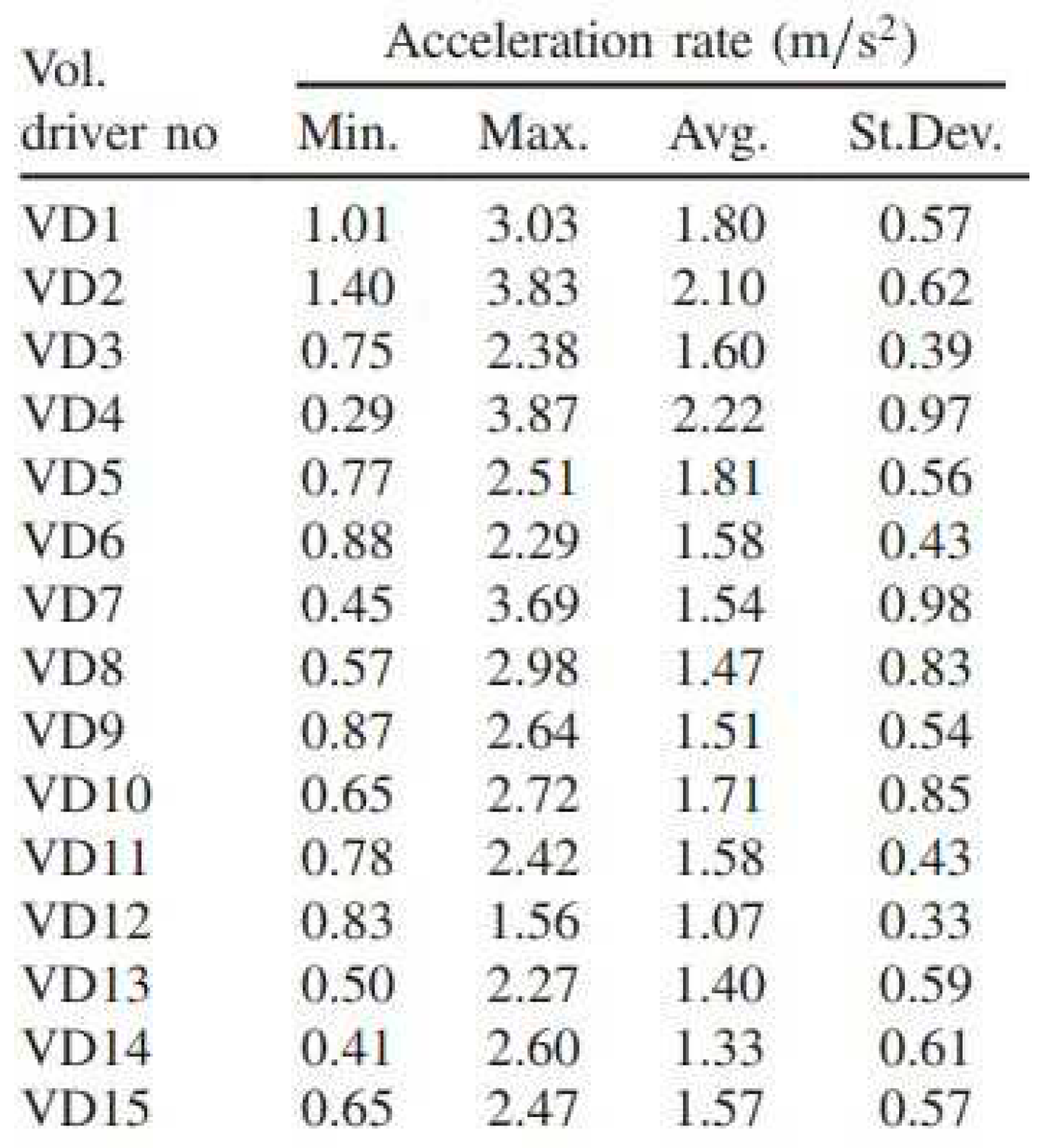
Figure 5.
(a) “Home screen” of the accelerometer software (b) “Record screen” where the user can choose the file format of the recordings.
Figure 5.
(a) “Home screen” of the accelerometer software (b) “Record screen” where the user can choose the file format of the recordings.
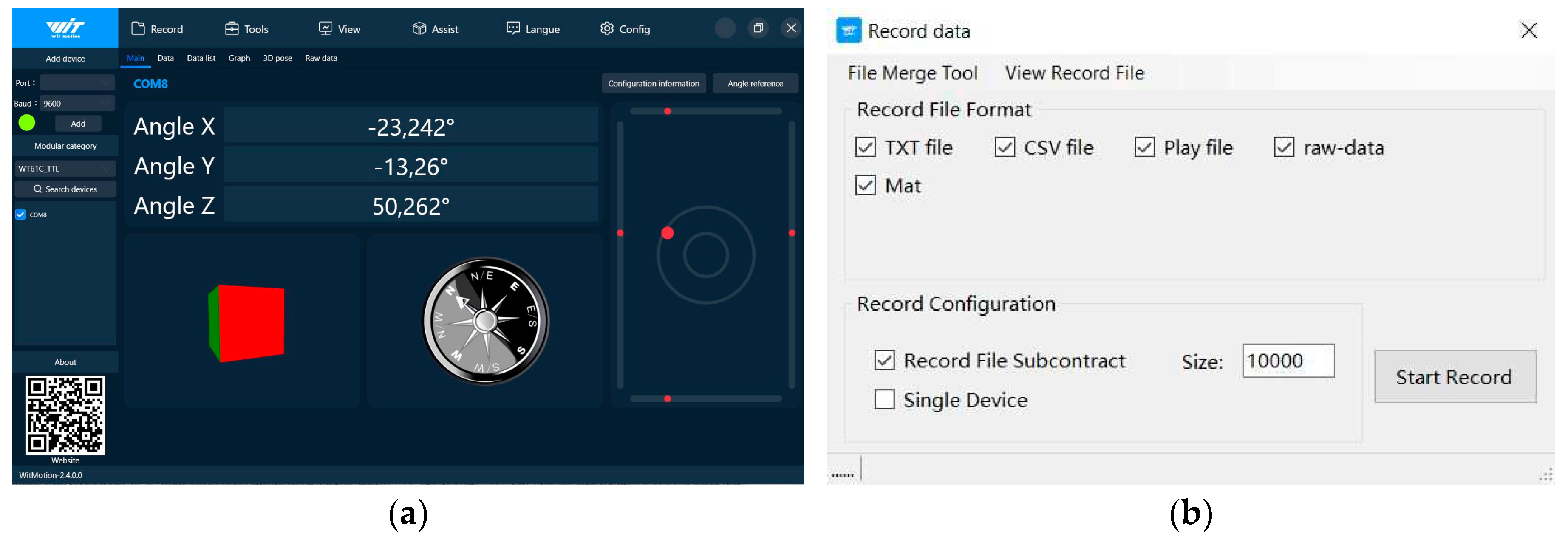
Figure 6.
Parking zones where the simulations took place. Respectively: (a) Coordinates 45°25'20.1"N 10°30'22.1"E; (b) Coordinates 44°31'46.9"N 11°20'03.7"E.
Figure 6.
Parking zones where the simulations took place. Respectively: (a) Coordinates 45°25'20.1"N 10°30'22.1"E; (b) Coordinates 44°31'46.9"N 11°20'03.7"E.
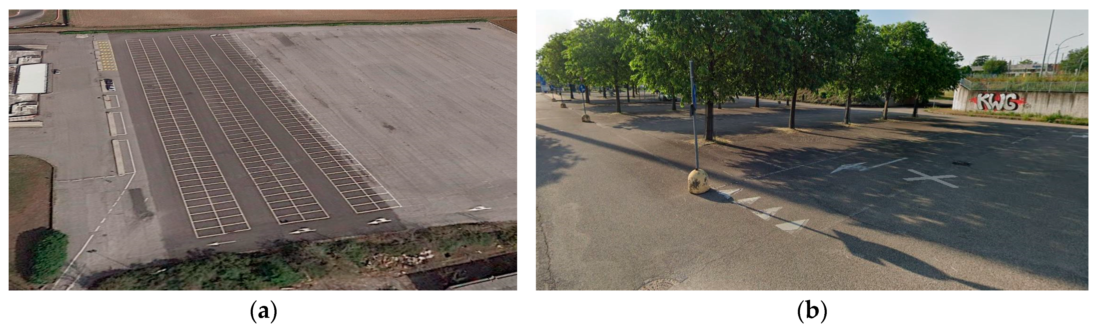
Figure 7.
Acceleration simulation schemes of the two parking zones displayed in: (a) Figure 6a; (b) Figure 6b.
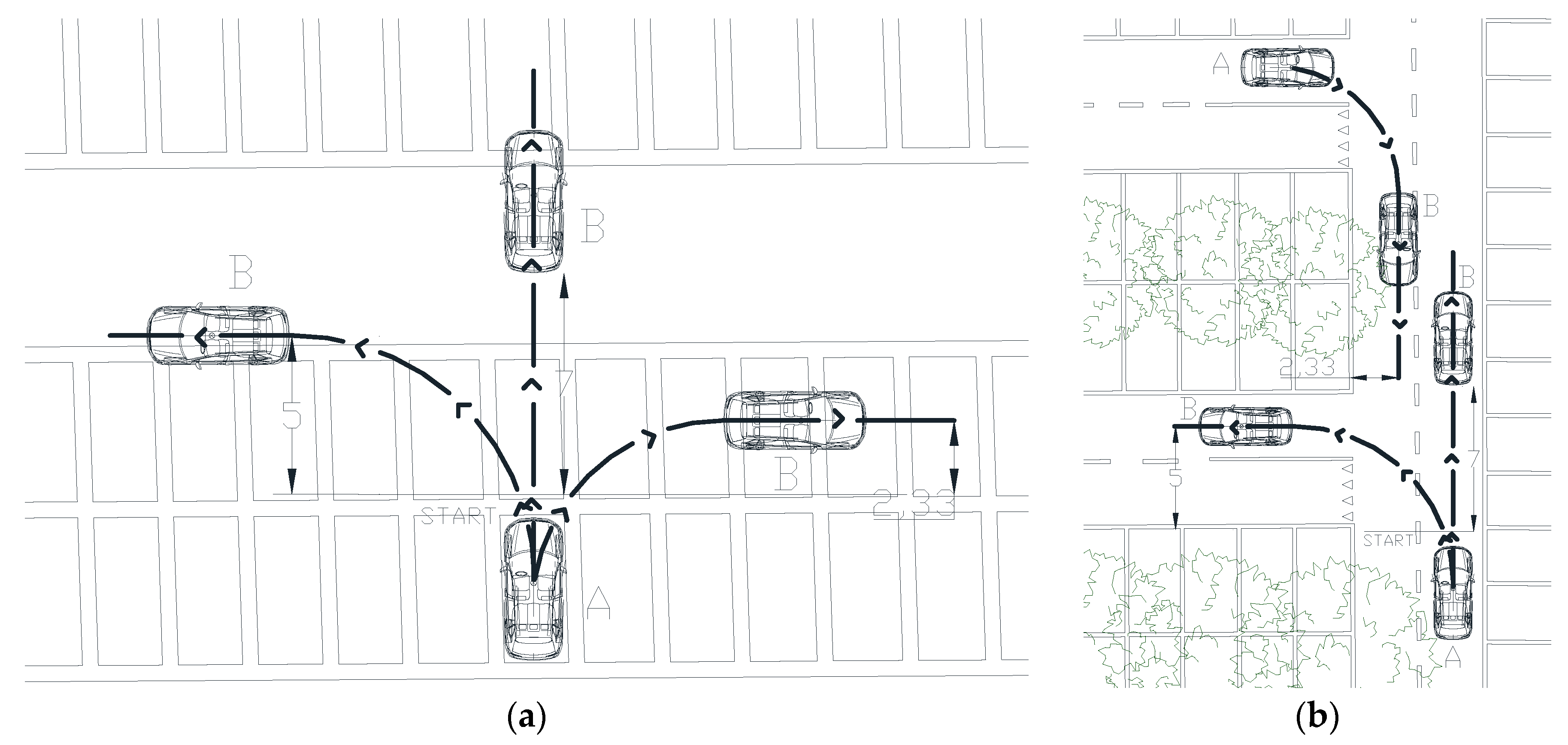
Figure 8.
MATLAB matrix where the sensor software automatically gathers the measurements.
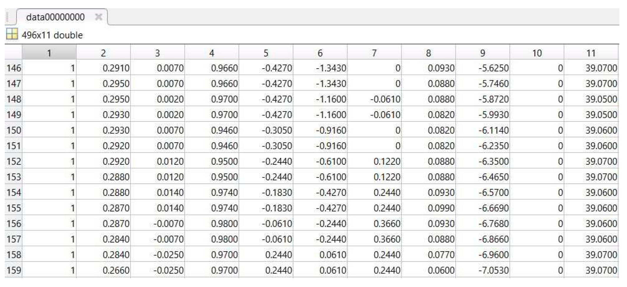
Figure 9.
Planar accelerations plot from a quick start test.
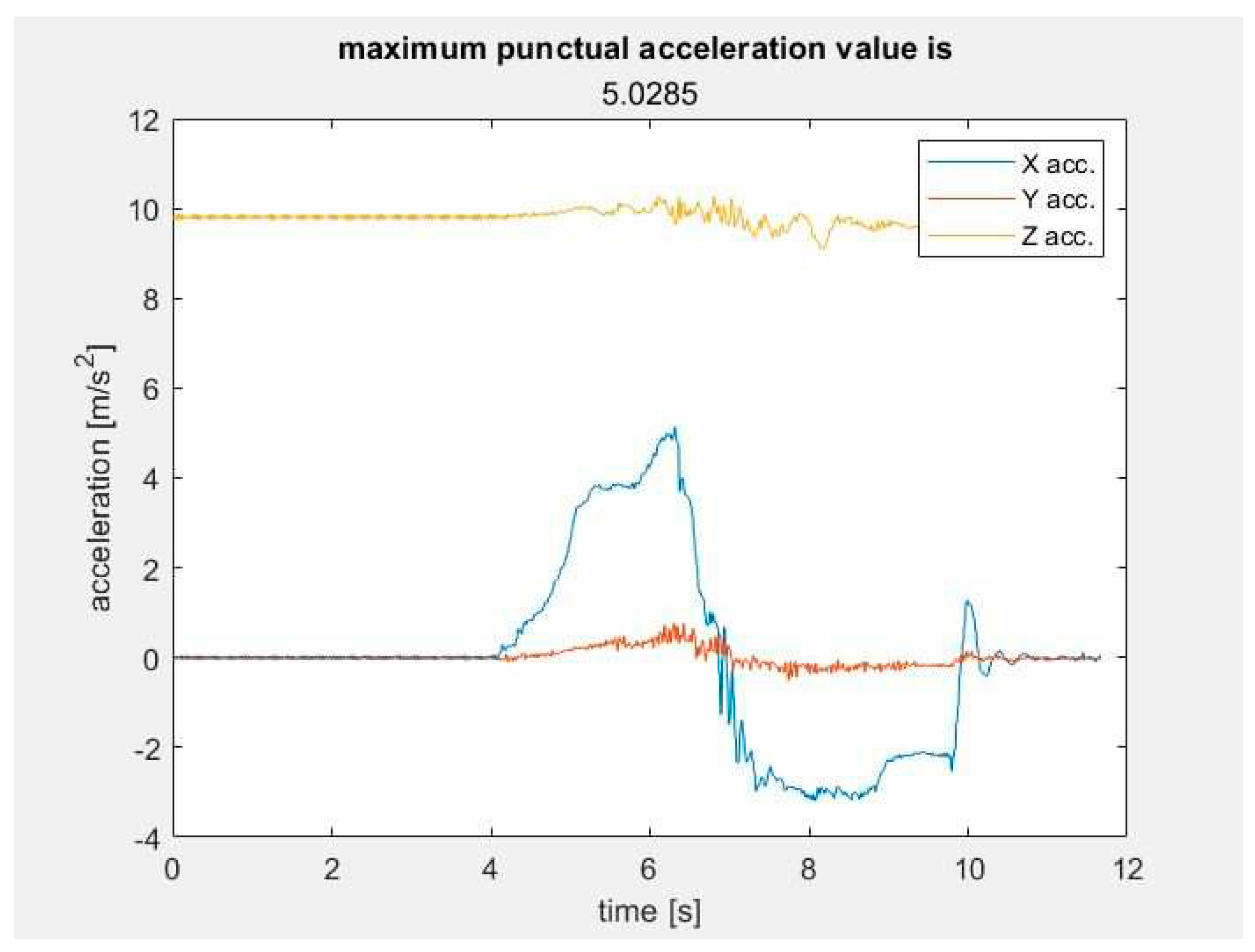
Figure 10.
Filtered planar accelerations from Figure 9.
Figure 10.
Filtered planar accelerations from Figure 9.
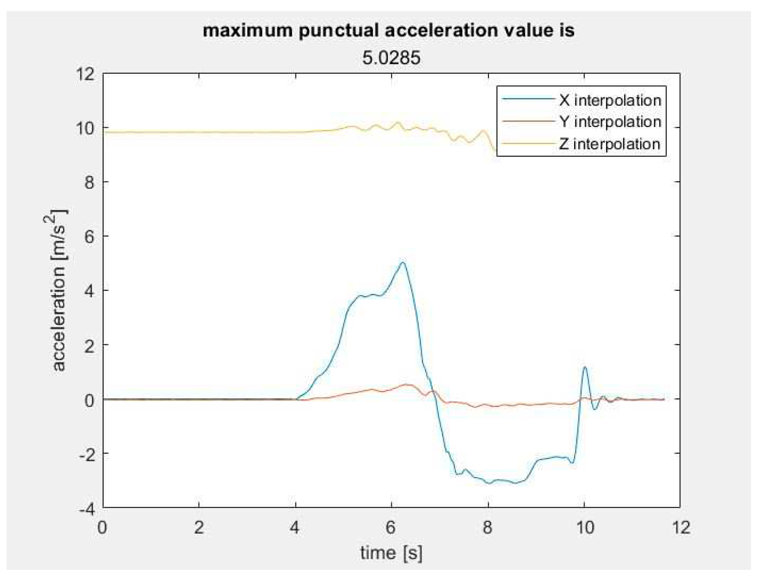
Figure 11.
Plot of the acceleration values sampled.
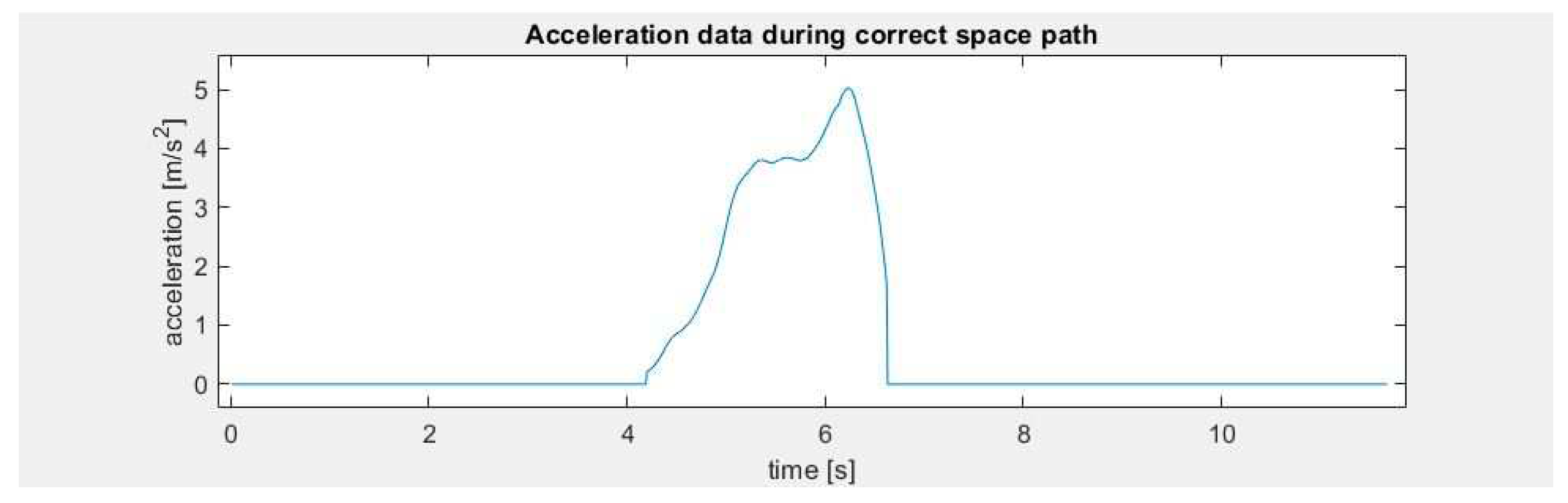
Figure 12.
Excel table reporting all the results.
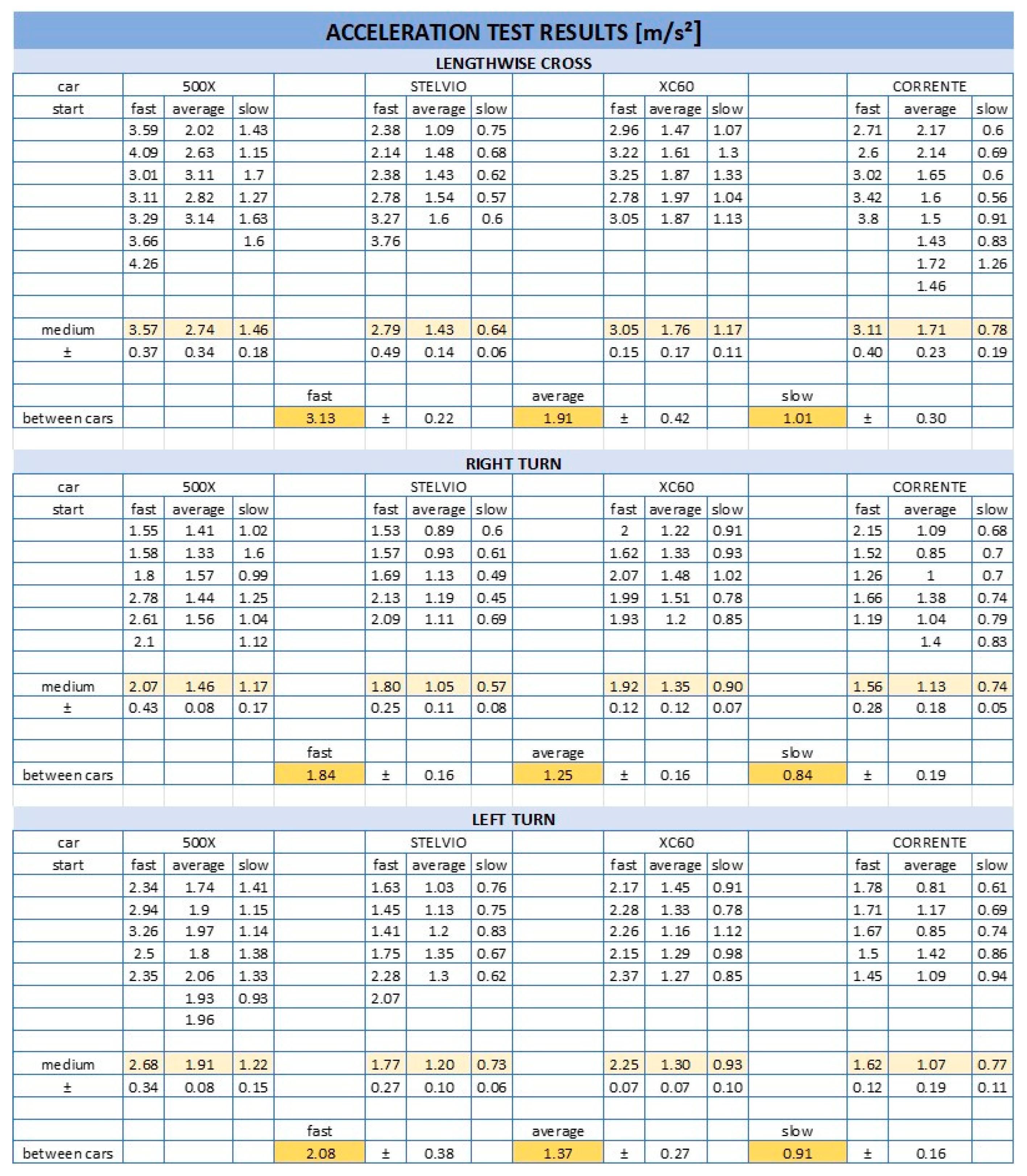
Table 1.
Data results reported from Murro [6] (p. 23).
Table 1.
Data results reported from Murro [6] (p. 23).
| Maneuver type | Start | Acceleration [m/s²] |
|---|---|---|
| Right turn | Slow | 0,57 ÷ 1,06 |
| Average | 0,91 ÷ 1,62 | |
| Quick | 1,43 ÷ 2,41 | |
| Left turn | Slow | 0,68 ÷ 1,20 |
| Average Quick |
1,05 ÷ 1,72 1,64 ÷ 2,65 |
|
| Lengthwise cross | Slow | 0,83 ÷ 1,49 |
| Average | 1,26 ÷ 2,05 | |
| Quick | 2,05 ÷ 3,11 |
Table 3.
Distances results.
| Incoming vehicle speed | Lengthwise cross | Right turn | Left turn |
|---|---|---|---|
| 30 km/h | 22,9 m | 28,8 m | 33,5 m |
| 50 km/h | 38 m | 48 m | 55,9 m |
| 70 km/h | 53,3 m | 67,1 m | 78,1 m |
| 90 km/h | 68,5 m | 86,3 m | 100,5 m |
Disclaimer/Publisher’s Note: The statements, opinions and data contained in all publications are solely those of the individual author(s) and contributor(s) and not of MDPI and/or the editor(s). MDPI and/or the editor(s) disclaim responsibility for any injury to people or property resulting from any ideas, methods, instructions or products referred to in the content. |
© 2023 by the authors. Licensee MDPI, Basel, Switzerland. This article is an open access article distributed under the terms and conditions of the Creative Commons Attribution (CC BY) license (http://creativecommons.org/licenses/by/4.0/).
Copyright: This open access article is published under a Creative Commons CC BY 4.0 license, which permit the free download, distribution, and reuse, provided that the author and preprint are cited in any reuse.


