
Submitted:
13 November 2023
Posted:
14 November 2023
You are already at the latest version
Abstract
In the field of computational fluid dynamics (CFD) for rotorcraft, two significant challenges are resolving the complex vortex structures in rotor wakes, and representing the moving rotor blades in the ambient airflow. This study addresses the first challenge by using a third-order unstructured finite volume solver, which, compared to its second-order counterpart, has substantially lower dissipation. Consequently, even relatively coarse meshes are capable of resolving small vortices. With this background flow field solver, the second challenge is addressed by modeling each rotor as an Actuator Disk Model (ADM), or describing individual rotor blades as actuator lines, designated as the Actuator Line Model (ALM). Both of these models are equipped with an improved correction for aerodynamic losses at blade tips, which is thoroughly presented in the methodology section. The numerical experiments section centers on analyzing errors linked to various sampling approaches. Additionally, the article discusses comparisons between vortex theory and ALM, specifically regarding calculations for fixed-wing aircraft. Furthermore, high-order precision and parallel efficiency are exemplified in scenarios encompassing rotors engaged in both hovering and forward flight rotors. The results in this paper demonstrate that the combination of the ALM/ADM with the improved tip loss correction and the third-order finite volume solver presents a new way of developing efficient tools for the aerodynamic analysis of helicopter rotors.
Keywords:
actuator line model
; actuator disk model
; tip loss correction
; high-order finite volume unstructured solver
1. Introduction
The simulation of helicopter rotors has always been a difficult task in aviation. Moving overlapping grid computational techniques developed in the researches [1,2,3] have shown to be successful. However, they require a significant amount of computational resources, intricate geometric modelling, and a huge number of grid cells, particularly boundary layer cells. Modelling discrete blade elements as momentum sources is an appealing strategy to drastically save computational costs [4]. The Actuator Line Model (ALM) and the Actuator Disk Model (ADM) have been introduced in the work [5]. These models have been widely used in simulating wind turbines with incompressible flow solvers [6]. This paper aimed to expand and improve the use of these models for helicopter rotor simulations with compressible flow solvers.
The ADM regards the time average of swept area of the blade as a source of momentum. In contrast, the ALM represents blade motion by placing the momentum source at changeable actuator lines in time. Control volumes surrounding actuator points are used to distribute body force in order to reduce numerical instabilities and transform sectional force into body force. Usually, a projection function with a Gaussian shape is used since it is simple and easy to construct. A lot of studies have examined applications of these two models, focusing in particular on the critical parameters influencing their results [6,7]. The projection radius has been identified as a crucial parameter. When , it leads to an inadequate vortex strength relative to actual values, resulting in an underestimated downwash velocity at the blade tip region and, consequently, an overestimation of lift. However, to keep numerical stability, it is important that , causing a large number of grid cells when , which damages the computational cost-effectiveness advantage of the models. The isotropic spherical volume force projection used by the standard ALM is obviously not reasonable for the real load distribution along the blade span. In particular, when the number of actuator points is insufficient , the projection may lead to computational instability. We have adopted the advanced ALM developed in the work [8], which successfully resolves this issue and expands it to ADM in this article. Discussions are held regarding normalisation functions [9] which guarantees that the sum of weighting functions close to the tip equals one, producing numerical results that are more consistent. An integral sampling strategy is compared with the point sampling strategy which is used widely.
In particular, the development of tip correction methods has been a research emphasis to improve the benefits of actuator models and get more accurate results on coarser grids, especially in the context of ALM. As an illustration, consider the Prandtl correction [10], which can occasionally result in lift values that are underestimated due to its empirical character. In contrast to techniques that depend on chord length , Jha [11,12] presented an elliptical distribution for the ALM projection radius, requiring less grid cells. It might, however, show numerical instability close to the blade tip and present difficulties when extending to ADM. Although vortex-based correction has recently been devised [13], its demanding assumptions and intricate computing techniques make it unsuitable for extension to rotor computations. Son [14] developed a tip correction method for ADM. Additionally, A filtered ALM [15] was first used in fixed-wing applications and has been expanded to wind turbine simulations, using a finite difference methodology. It gives a effective way to use ALM on coarser grids, but this method employs a finite difference approach that leads to lift overestimations at the blade tip section. To deal with shortcoming, we present a improved correction based on it by adding ghost sections and successfully extend the improved correction to both ALM and ADM in this study.
High-order methods perform well in simulation containing rotorcraft, because of the need to capture complex flow structures such as tip vortices. For these kinds of simulations, finite difference methods based on structured grids have been widely used. Nevertheless, these structured grid solvers usually require substantial preprocessing and present formidable obstacles when working with intricate geometries. As a result, unstructured solvers have become a more flexible option for solving these problems. Efforts have been made to extend ALM and ADM models within commercial software such as CFX [7] and StarCCM+ [16,17]. However, conventional second-order unstructured solvers often product significant numerical dissipation and the complex structures of tip vortices can be smeared by its numerical dissipation, which can reduce the accuracy of the results. Furthermore, to resolve these problems, more grid cells are needed or high-order methods are used. High-order unstructured solvers can be roughly divided into two main classes: the first one is based on high-order finite volume methods [18] and the second one is based on discontinuous Galerkin methods [19,20]. We used a high-order unstructured solver [21] which is coded in the framework of OpenFOAM [22], which is based on implicit third-order compact finite volume methods. The solver with models presented in this article enabled us to address the challenges associated with rotor computational fluid dynamics more effectively.
The rest of this article is organised as follows: The methods of governing equations, spatial discretization and temporal discretization are introduced in Section 2.1. For an overview of advanced ALM and ADM models, see Section 2.2. The tip correction techniques refined in this paper are presented in Section 2.3. The implementation algorithm is shown in Section 2.4. The numerical experiments carried out in this work are discussed in Section 3. The conclusion is finally given in Section 4.
2. Numerical Methodology
2.1. Flow Solver
2.1.1. Governing Equations
In this article, the numerical tests are simulation of compressible flows governed by Reynolds averaged Navier-Stokes (RANS) equations, and the Spalart Allmaras (SA) one-equation model is used. The non-dimensional forms of the compressible RANS-SA equations can be expressed as
where
In Equation (2), is the conservative variables, and are the convective flux and viscous flux, respectively. and are the free steam Mach and Reynolds numbers. Furthermore, represents the source term. The velocity are the velocity of the flow field. is introduced in following sections. For the calculation of the convective flux, viscous flux and source term about the turbulent variable, we employ the SA-neg model [23].
The viscous stress tensor can be represented in vector notation as
The thermal conductivity, denoted as , is described by
where represents the specific heat at constant pressure, and is the coefficient for laminar kinetic viscosity evaluated through the Sutherland law
in which and . The laminar Prandtl number is indicated as , while the turbulent Prandtl number is .
2.1.2. Spatial and Temporal Discretization
To find the influence of high-order solvers on rotorcraft aerodynamics, a second-order solver based on Gauss linear reconstruction () and a third-order solver based on implicit variational reconstruction () were employed. Both of the two solvers are implemented in the framework of OpenFOAM [22]. To avoid the influence of the temporal discretization, a third-order implicit dual-time stepping method is used. Here, we will focus on the third-order solver.
In Figure 1, within the elements, conserved quantities are represented using degree p piece-wise polynomials
The non-dimensional Taylor basis functions can be founded in [21]. The coefficients of the solution polynomials can be determined through a variational reconstruction. The cost functions employed in this approach offer flexibility, and the specific cost function utilized in this article is defined as
where is selected according to [21]. The coefficients of these polynomials are determined by solving a system of linear equations
in which denotes the neighbor cells sharing the interfaces with the current cell. The specific forms of the matrices are
The method we utilize to solve this linear system is the symmetric Gauss-Seidel (SGS) iterative method as
To achieve third-order accuracy approximation, a sufficient number of Guass-Legendre points is required to evaluate values related to the quadratic polynomials. For convective flux and diffusive flux in Equation (1), computation over all Guass-Legendre points on the interfaces is needed. When solving source terms, evaluation of values at each volume Guass-Legendre points is necessary.
The temporal discretization employed is the third-order singly-diagonally implicit Runge–Kutta (SDIRK) method as presented by [24]. The Equation (1) is integrated in time according
The and is computed in the pseudo-time stepping inner iteration using
The values of and can be found in [25]. In the implicit inner iteration step s, the reconstruction iteration in Equation (7) is resolved once before an inner iteration step which employs the matrix-free LU-SGS approach, as proposed by [26]. In this article, the maximum of inner iteration steps is set 20. The coupled technology makes the convergence of reconstruction and inner iteration synchronously, which can reduce the computational cost obviously. It provides a third-order numerical accuracy, which is consistent with the spatial discretization accuracy used in this study. For more extensive details regarding the implementation of the third-order solver, please refer to [21].
2.2. Advanced Actuator Line/Disk Modeling
Actuator line and actuator disk models were integrated with each of the two solvers for comparative analysis. In this section, we will first introduce the standard ALM as well as the recently developed advanced ALM. As shown in Figure 2, the former applies the volume force source terms of segmented blade elements to the control volumes using an isotropic Gaussian projection method, with the projection domain being a spherical shape. In contrast, the latter employs a linear distribution along the blade span, addressing the issue of inconsistency between the model and the actual force distribution. This inconsistency becomes particularly noticeable, especially when the density of force distribution is low at certain locations along the span, such as at the actuator points.
For the standard ALM, the volume force density at the center of the control volume for the mth actuator point (aerodynamic point at 1/4 chord length) on the nth blade can be represented as
The projection function is denoted as
Here, represents the distance between the control volume center and the actuator point. is the Gaussian projection radius and the projection function decays to of its maximum value when . Therefore, the number of control volumes corresponding to each actuator point is finite, ensuring that the computational cost required for ALM and ADM is limited.
The projection function for advanced ALM can be expressed as
where represents the spacing between actuator points, the distance from the center of the control volume to the actuator line of the corresponding control point on the blade can be expressed as
Additionally, is defined as
where . For the control volume center radial coordinates , they must satisfy . Special considerations need to be taken into account, and for root region of the first actuator point and tip region of the last actuator point . Compared to the standard Actuator Line Model, the projection domain of this model follows a cylindrical distribution, and the linear radial distribution is more reasonable.
To prevent numerical instability caused by insufficient grid resolution or projection function volume integrals less than unit at the root and tip of blades, it’s necessary to normalize the Equation (10), denoted as
The calculation of loads on the segmented rotor blades is determined by
When , it corresponds to ALM. However, if exceeds , it corresponds to ADM, where the right-hand term introduces a time-averaging effect. In the case of using ADM, is typically chosen. Additionally, the calculations of blade element force in Figure 3 are based on
For a blade element, c is the local chord length. The lift coefficient and drag coefficient of the segmented 2D airfoil can be obtained based on experimental results and tables generated by the XFLR5 software [27] respectively. and are the unit vectors of the local coordinate system of blades. is evaluated according to the sampled velocity and rotor motion velocity, which is required for the computation of parameters such as the angle of attack , Mach and Reynolds number .
Two velocity sampling methods are discussed in this article. The first sampling method is the widely-adopted point sampling, which requires searching the nearest control volume and employing gradient interpolation to determine velocities at the actuator points. The second method involves the integration of control volume cells surrounding the actuator points, utilizing a projection function denoted as
Subsequent numerical experiments in the following sections demonstrate that the latter approach yields more stable and accurate sampling results.
2.3. Improved Tip Loss Correction
Studies [7,16] have shown that the parameter in the ALM projection function has an impact on the vortex core scale near the blade tip. While projection with can produce reasonable vortex core scale, it required grid size satisfying to reduce numerical error due to insufficient resolution. Consequently, it is likely to underestimate the blade-tip vortex core scale for relatively coarse grids and overestimate lift coefficients. We improve the correction of filtered ALM originally proposed by [15] and extend its application to rotor aerodynamic calculations utilizing advanced ALM and ADM. The improved correction guarantees the accuracy of load calculation in simulations with coarse grids.
Following the approach described in [15], this article corrects the sampled velocities in the flow field. Initially, the free stream velocity is obtained by , removing the influence of the vortex core scale . The computation of circulation G from the lift in the previous time step according to
The finite difference of in [15] is computed using
The original finite difference approach leads overestimation of lift coefficients around the blade tip for rotorcraft. We take the finite differences at the interfaces of sections rather than centres and add ghost section to keep the circulation G to be zero at both ends of blades, which effectively mitigates the problem of insufficient downwash velocity in the tip section correction. The improved correction using the finite difference according to
In this process, the improved differential approach is used in Figure 4, adding ghost sections at both ends, where and . The value of ghost sections is opposite values of the inner sections. The tip loss correction is employed to calculate the new downwash velocity components based on and :
Because the solver employs a dual-time stepping inner iteration approach, the correction can be performed only once to update the downwash velocity during every pseudo time step. Through calculations, it is found that the corrected velocity computed by
converges rapidly when . Since the number of actuator points is small, this method does not significantly increase the computational cost. This correction method can be used in both in ALM and ADM, and the . Furthermore, because the loads are time-averaged, the resulting vortex strength is significantly lower than ALM, thus for projection has minimal impact on the actual vortex strength, and is set in the correction procedure of ADM.
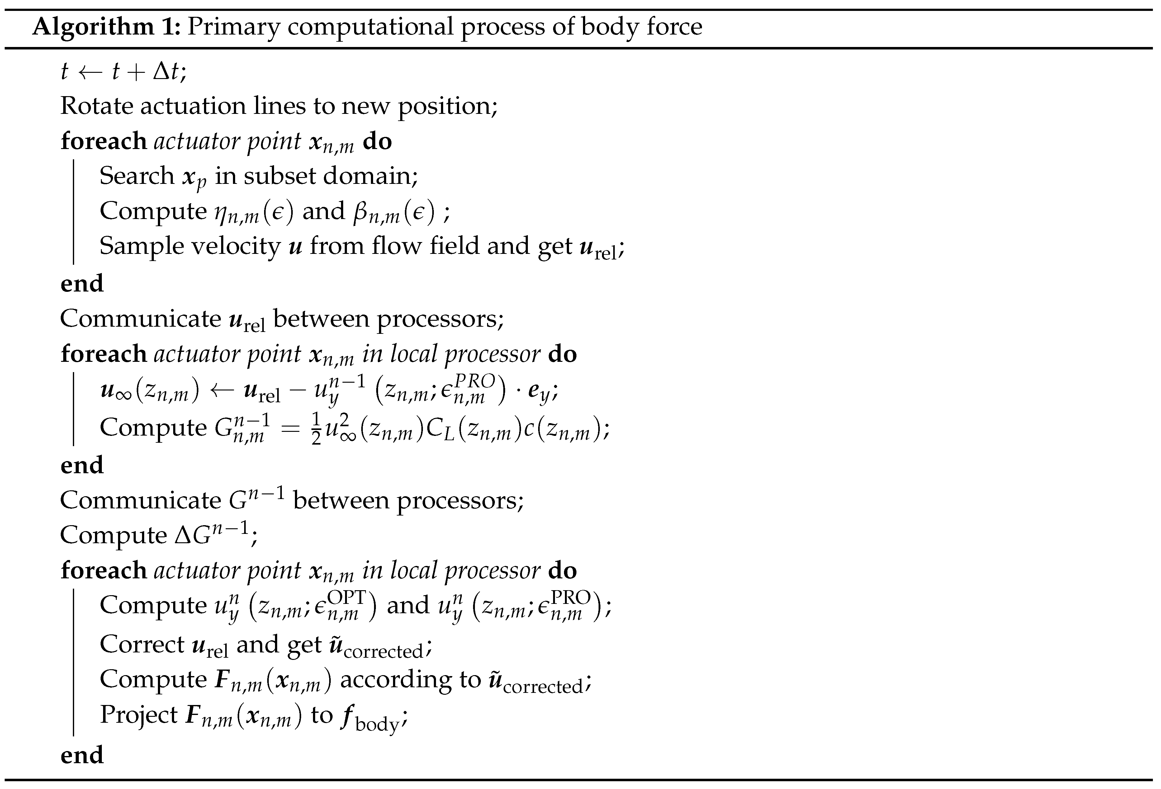
2.4. Implementation
Algorithm 1 mentions primary computational process of body force. At the beginning of computation, a cylindrical subspace can be defined based on the location of the rotor, and generate a KDTree which improves search complexity according to the control volumes in the subspace, which enhances the computational efficiency of models [28]. Unlike ALM representing moving blades, ADM doesn’t require further position of actuator points updates. During correction procedure, for ALM and for ADM. Subsequent numerical experiments demonstrate that this implementation can achieve high parallel efficiency.
3. Results and Discussion
3.1. Two-Dimensional Infinite Wing
In this section, tests were conducted by simulating a two-dimensional infinite wing to analyze and compare the differences between two-dimensional NACA0012 airfoil and two-dimensional ALM. Furthermore, the influence of the two sampling methods with different parameter of the ALM on calculation errors was investigated.
In Figure 5, the mesh of airfoil is compared with the mesh of the ALM. In the ALM mesh, a circular region with a radius of is refined with , and . The free stream Mach number is 0.2, the angle of attack degrees, and the lift coefficient is approximately 1. In Figure 6, by comparing the computed Mach number contours, it is evident that the projection radius affects the calculation results. When , the Mach number contours of the two-dimensional ALM are close to the results of the two-dimensional airfoil.
This test primarily compares the errors of the two sampling methods performed with the two solvers, mainly based on the comparison of velocity magnitude and velocity angle of attack. Figure 7 demonstrates that the error of the point sampling method varies with and . It is clear that, compared to , has a more significant impact on the error, and the third-order solver has greater advantages in convergence of accuracy.
Figure 8 presents the error of the integral sampling method as it varies with and . By comparing with Figure 7, it can be observed that the integral sampling method provides more robust and accurate sampling results. Therefore, the default sampling method in this article is integral sampling, and to control the impact of sampling methods on results, is recommended.
3.2. Three-Dimensional Finite Wing
3.2.1. Constant Circulation Rectangular Wing
This test simulates a finite-length fix wing with a fixed circulation distribution to demonstrate the effectiveness of the tip loss correction presented in this article. The rectangular wing has a chord length of with a fixed lift coefficient , a span of . The free stream whose Mach number , and the Reynolds number . A constant circulation distribution along the span is given by .
According to vortex theory used in [7], we can obtain a theoretical reference solution for the downwash velocity, denoted as
where z is the spanwise coordinate with the wing’s center as the origin point. The vortex core radius, , is typically between to of the chord length c, as per common research practices. , mentioned in [7], yields results close to . To highlight the advantages of the ALM model used in this article, , and are selected.
Figure 9 shows the mesh used in this case, and refinement around the wing with a spacing of is done. Figure 10 displays the results obtained with two different solvers. It is evident that the tip correction effectively calculates the downwash velocity near the tip without reducing the projection radius to . The improved tip loss correction presented in this article yields better result when contrasted with the original correction in [15]. Furthermore, at the middle span of wing, the downwash velocity of the third-order solver agrees with the theoretical reference solution better than the result of the second-order solver. The Q-criterion iso-surfaces and Mach number distribution in Figure 9 are obtained from the third-order solver’s ALM with tip loss correction, and they closely resemble the actual flow structures.
3.2.2. Elliptic Wing
This case is used to validate the ALM model for downwash velocity calculations on an elliptical wing, and theoretical solution can be obtained based on the vortex theory. It presents greater computational challenges compared to a fixed-chord rectangular wing because the chord length decreases to zero towards the tips. In the article [7], yielded results agree with solution of the vortex theory, but the grid size around tips where was limited due to the requirement of , resulting in a high computational cost. This article employs a fixed value for calculations with the improved correction, and gets expected results as presented in [7].
The computational mesh for this case is the same as shown in Figure 9, with a free stream . According to elliptical wing vortex theory, a constant downwash velocity along the span is represented by
In this work, , the chord length distribution follows
where wing span , and the lift coefficient of the airfoil is . The downwash angle can be computed by
To obtain the theoretical solution, an angle of attack , and the angle of attack of the incoming flow . Thus, a fixed lift coefficient can be achieved.
Figure 11 illustrates the results of the two solvers for the downwash velocity along the span in this case, the tip correction helps to obtain numerical solutions agree with the theoretical solutions. The original tip loss correction presented in [15] still underestimates downwash velocity for sections at both ends, whereas the improved tip loss correction effectively resolves this problem. Compared with the second-order solver, the third-order solver evaluate closer downwash velocity to the theoretical solution, which is mainly caused by the higher resolution for the vortex structures along the wing.
3.3. Hover Flight Rotor
In this paper, numerical simulations of blade loads and tip vortices for Caradonna-Tung rotor [29] are carried out. According to the experiment description, the rotor maximum radius , and the aspect ratio with chord length . The rotor has 2 blades with NACA0012 airfoil. In the simulations, the tip Mach number , and the Reynolds number . Simulations are performed for two different collective pitches, and with ALM and ADM separately. The boundary conditions of the computational domain are set to non-reflective boundary conditions, with velocity obtained from internal cells.
The computational mesh shown in the Figure 12 has a total hexahedral cell quantity of , and the mesh is refined around the rotor blade and its lower region to . Compared with the meshes used in [17], the mesh in this test has larger grid sizes, resulting in significantly lower computational costs for the simulation. The cells which are applied with momentum source calculated from ALM/ADM are marked. For both ALM and ADM equipped with the improved tip loss correction, we select for the projection function, and the actuator points spacing in this test. In order to guarantee the numerical stability, is used.
Figure 13 and Figure 14 show the Mach number contours of ADM calculated with blade collective pitches of and . Due to time-averaging, although the third-order solver captures more flow structures compared to the second-order solver, it still can not fully capture the expected tip vortex structures. Figure 15 and Figure 16, obtained with ALM, show the vorticity contours at iso-surface with blade collective pitches of and , and describe the evolution progress of the expected tip vortex structures. The vortex structures captured by the second-order solver only develops about for collective pitch and less than for collective pitch. The tip vortices produced by the rotor with collective pitch have higher vortex strength than the that of the rotor with collective pitch. By contrast, the age angle of vortex evolution with third-order solver are about three times than those with second-order solver. The computing time consumed for the simulation with third-order solver is about five times that of the second-order counterpart. Compared with mesh refinement to capture larger vortex age angle [17], using a high-order solver is a better choice when considering the increases in computational cost.
Figure 17 presents comparisons of sectional lift coefficient distribution along the rotor blade with collective pitches of and . The original correction [15] and the improved correction are employed with ALM and ADM separately. The results of the improved correction are in good agreement with the experimental data for both ALM and ADM, especially around the tip region. However, the original correction fail to produce expected results, and a considerable overestimation of the lift coefficient for the tip sections is made. Considering the tip load substantially contribute to the total loads of rotors, this results in larger error compared to fixed wing and wind turbine. To illustrate the advantage of the improved correction for load evaluation of rotors, the rotor lift coefficient obtained based on is presented in Table 1. Combining the results in Figure 17, it can be concluded that ALM yields slightly higher lift coefficients compared to ADM, but the errors are all controlled within in this test. In view of the relatively lower computational cost, the advanced ALM and ADM equipped with improved correction provide an attractive means to evaluate rotor blade loads in engineering.
Figure 18 shows comparisons of the ALM results of blade-tip vortex evolution in vertical and radial directions respectively, where the and represent the vertical position and the radial position. It can be found that the third-order solver, due to lower numerical dissipation, predicts a better agreement with the experimental results for the vortex age up to . However, the second-order solver can not predict expected vortex core positions, and the errors mainly occur when the vortex angle exceeds . With the increase of vortex age, the vortex strength decreases. The decrease of vortex strength is caused by both physical and numerical dissipation, and the numerical dissipation plays a leading role in this test. Compared with the error of radial position, larger error can be seen in the results of vertical position, because the results of downwash velocity also affect the vertical speed of blade-tip vortices.
3.4. Forward Flight Rotor
In the rotor-fuselage aerodynamic interaction experiment conducted at the Georgia Institute of Technology (GIT) [30], the rotor consists of two rectangular blades with radius and root cutting was . The blades used a NACA0015 airfoil and the chord length . The position and tilt angle of rotor are described in the schematic diagram of the experimental model shown in Figure 19. The computational domain is a cylinder with a radius and the cylinder diameter D of fuselage is . The tip Mach number of the rotor is , and the free stream Mach number varies with different advance ratios as and . The simulations are performed using 3,906,913 tetrahedral elements, as shown in Figure 20, and the gird sizes near the rotor and fuselage is refined to . The projection radius and is used in models. The improved tip loss correction is employed in both ALM and ADM, and the time step size is decided according to .
Simulations of two forward flight conditions of and are performed with the two solvers respectively. The ALM results of the vorticity contour at iso-surface are shown in Figure 21 and Figure 22. The vortex strength decreases fast in the results provided by second-order solver due to its larger numerical dissipation, and the expected blade-tip vortex evolution can not be found. By contrast, the vortex structures are presented with the third-order solver clearly, and the distances of vortex rings increase with the increase of advance ratios . The positions of interaction between vortices and the fuselage also vary according to different advance ratios.
Figure 23 shows comparisons of the time-averaged pressure coefficients on the top surface of the cylindrical fuselage between ADM and ALM over the one period against experimental results. All the numerical results agree well with the experimental data, it is obvious that the interaction of downwash flow and fuselage can be predicted with all the four methods. The primary error is produced at the front of the fuselage due to the overlap between the fuselage and the projection of the volume force, leading to higher pressure coefficients. A potential approach can be utilized to resolve the problem with introducing an anisotropic volume force distribution that aligns better with the actual physical model.
We perform a scaling test running on the high performance computing platform provided by Beihang University to show the parallel scaling efficiency of the third-order solver combined with ALM on the same mesh of this case. Each computing node in the cluster comprises two Intel Xeon Gold 6240 processors, with a maximum of 32 cores per node and a maximum test core count of 256. Figure 24 illustrates the results with a parallel efficiency of up to 15261 cell per core, whereas the parallel efficiency decreases to with methods based on moving overlapping grids due to the need to update the position of body-fitted grid around the blades in [16]. The results in [21] show that the third-order solver has high parallel efficiency and excellent scalability, and the ALM can keep the advantage of the solver.
4. Conclusions
In this work, we developed the combination of advanced ALM/ADM and a third-order unstructured finite volume solver for helicopter rotors. In simulations using this method, there is no need to model complex geometric and employing the moving overlapping grid technology which is computational expensive. An improved tip loss correction have been developed and eliminates the strict requirements of grid size satisfying when modeling a reasonable vortex core scale with , which means that coarser grids can be used. The comparison of two sampling methods show that the third-order solver products less error for the same in the projection function of models with the integral sampling method, and the presented improved tip loss correction performs better than the original correction in fixed-wing and rotor tests. The numerical results of both ALM and ADM agree with experimental results of sectional lift coefficients in the hover flight rotor, and the rotor-fuselage aerodynamic interaction in the forward flight rotor. The ALM replaces a moving blade with an array of actuator points in flow, and tip vortex structures are captured by the model. However, expected tip vortex positions can not be calculated with the conventional second-order solver due to its high numerical dissipation. The third-order solver is employed to resolve the problem without the need of mesh refinement, providing sufficient resolution for vortex structures. The results also demonstrate that the solver can be used on unstructured meshes as well as having high parallel efficiency and excellent scalability. Therefore, the method helps researchers to study blade loads and downwash airflow with relatively low computational cost for rotorcraft aerodynamics.
Finally, the method is competent to simulate flows containing tip vortex structures. In the preliminary design of tiltrotors, the tool can be employed to simulate various rotor-rotor, rotor-wing, and rotor-tail aerodynamic configurations. Poor configurations product harmful aerodynamic interaction leading to decreased rotor aerodynamic efficiency, wing lift-to-drag ratio, and stability. Furthermore, simulating the coupling of ship/rotor airflow is also a promising application situation, where the complex aerodynamic interaction between rotor and ship have a significant effect on the landing security of helicopters.
Author Contributions
Conceptualization, M.Y. and S.L.; methodology, M.Y.; software, M.Y. and W.P.; validation, M.Y. and W.P.; formal analysis, M.Y. and W.P.; investigation, M.Y. and W.P.; resources, M.Y. and W.P.; data curation, M.Y.; writing—original draft preparation, M.Y.; writing—review and editing, M.Y., W.P., and S.L.; visualization, M.Y.; supervision, W.P. and S.L.; project administration, S.L.; funding acquisition, S.L. All authors have read and agreed to the published version of the manuscript.
Funding
This research was funded by the National High-Tech R&D Program of China (863 Program), grant number 2012AA112201.
Data Availability Statement
The data presented in this article are all generated from the source code publicly available in our GitHub repository at https://github.com/buaaymh/AeroFOAM, accessed on 3 November 2023
Acknowledgments
The authors would like to express their deepest appreciation to the high-performance computing platform provided by Beihang University.
Conflicts of Interest
The authors declare no conflict of interest. The funders had no role in the design of the study; in the collection, analyses, or interpretation of data; in the writing of the manuscript, or in the decision to publish the results.
Abbreviations
The following abbreviations are used in this manuscript:
| ALM | Actuator Line Model |
| ADM | Actuator Disk Model |
| RANS | Reynolds Averaged Navier-Stokes |
| SA | Spalart Allmaras |
| SGS | Symmetric Gauss-Seidel |
| SDIRK | Singly-Diagonally Implicit Runge–Kutta |
| Re | Reynolds number |
| Ma | Mach number |
| body force applied on control volumes | |
| blade force of the mth section of the nth blade | |
| projection weight of blade force of the mth section of the nth blade | |
| Gaussion projection raduis | |
| grid size | |
| spacing between actuator points | |
| coordinate of of control volume center | |
| coordinate of actuator point of the mth section of the nth blade | |
| coordinate of blade root | |
| coordinate of blade tip | |
| radial coordinate of control volume center | |
| radial coordinate of actuator point of the mth section of the nth blade | |
| radial coordinate of blade root | |
| radial coordinate of blade tip | |
| distance to the actuator line | |
| radial distance over spacing between actuator points | |
| volumetric normalization factor of the mth section of the nth blade | |
| blade sectional lift coefficient | |
| blade sectional drag coefficient | |
| number of blades | |
| number of actuator lines | |
| c | local chord |
| relative angle of attack of a blade section | |
| relative velocity | |
| sampled velocity | |
| corrected velocity | |
| circulation computed form previous step | |
| finite difference of circulation | |
| rotor thrust coefficient | |
| advance ratio |
References
- Steijl, R.; Barakos, G.; Badcock, K. A CFD framework for analysis of helicopter rotors. In Proceedings of the 17th AIAA computational fluid dynamics conference; 2005; p. 5124. [Google Scholar]
- Ganti, Y.; Baeder, J. CFD analysis of a slatted UH-60 rotor in hover. In Proceedings of the 30th AIAA Applied Aerodynamics Conference; 2012; p. 2888. [Google Scholar]
- Jain, R. Hover Predictions on the S-76 Rotor with Tip Shape Variation Using Helios. J. Aircr. 2018, 55, 66–77. [Google Scholar] [CrossRef]
- Guntupalli, K.; Rajagopalan, R.G. Development of discrete blade momentum source method for rotors in an unstructured solver. In Proceedings of the 50th AIAA Aerospace Sciences Meeting including the New Horizons Forum and Aerospace Exposition; 2012; p. 422. [Google Scholar]
- Mikkelsen, R. ; others. Actuator disc methods applied to wind turbines. PhD Thesis, Technical University of Denmark, 2003.
- Martinez, L.; Leonardi, S.; Churchfield, M.; Moriarty, P. A comparison of actuator disk and actuator line wind turbine models and best practices for their use. In Proceedings of the 50th AIAA Aerospace Sciences Meeting including the New Horizons Forum and Aerospace Exposition; 2012; p. 900. [Google Scholar]
- Shives, M.; Crawford, C. Mesh and load distribution requirements for actuator line CFD simulations. Wind Energy 2013, 16, 1183–1196. [Google Scholar] [CrossRef]
- Jha, P.K.; Schmitz, S. Actuator curve embedding—An advanced actuator line model. J. Fluid Mech. 2018, 834, R2. [Google Scholar] [CrossRef]
- Churchfield, M.J.; Schreck, S.J.; Martinez, L.A.; Meneveau, C.; Spalart, P.R. An advanced actuator line method for wind energy applications and beyond. In Proceedings of the 35th Wind Energy Symposium; 2017; p. 1998. [Google Scholar]
- Shen, W.Z.; Mikkelsen, R.; Sørensen, J.N.; Bak, C. Tip loss corrections for wind turbine computations. Wind Energy 2005, 8, 457–475. [Google Scholar] [CrossRef]
- Jha, P.; Churchfield, M.; Moriarty, P.; Schmitz, S. Accuracy of state-of-the-art actuator-line modeling for wind turbine wakes. In Proceedings of the 51st AIAA Aerospace Sciences Meeting including the New Horizons Forum and Aerospace Exposition; 2013; p. 608. [Google Scholar]
- Jha, P.K.; Churchfield, M.J.; Moriarty, P.J.; Schmitz, S. Guidelines for volume force distributions within actuator line modeling of wind turbines on large-eddy simulation-type grids. J. Sol. Energy Eng. 2014, 136, 031003. [Google Scholar] [CrossRef]
- Kleine, V.G.; Hanifi, A.; Henningson, D.S. Non-iterative vortex-based smearing correction for the actuator line method. J. Fluid Mech. 2023, 961, A29. [Google Scholar] [CrossRef]
- Son, C.; Kim, T. Actuator Disk Model with Improved Tip Loss Correction for Hover and Forward Flight Rotor Analysis. Aerospace 2023, 10, 494. [Google Scholar] [CrossRef]
- Martínez-Tossas, L.A.; Meneveau, C. Filtered lifting line theory and application to the actuator line model. J. Fluid Mech. 2019, 863, 269–292. [Google Scholar] [CrossRef]
- Merabet, R.; Laurendeau, E. Hovering helicopter rotors modeling using the actuator line method. J. Aircr. 2022, 59, 774–787. [Google Scholar] [CrossRef]
- Zhang, C.; Xu, G.; Shi, Y. Investigation of a Virtual Blade Method for Aerodynamic and Acoustic Prediction of Helicopter Rotors. Int. J. Aeronaut. Space Sci. 2023, 24, 381–394. [Google Scholar] [CrossRef]
- Ji, Z.; Liang, T.; Fu, L. High-Order Finite-Volume TENO Schemes with Dual ENO-Like Stencil Selection for Unstructured Meshes. J. Sci. Comput. 2023, 95, 76. [Google Scholar] [CrossRef]
- Pei, W.; Jiang, Y.; Li, S. An Efficient Parallel Implementation of the Runge–Kutta Discontinuous Galerkin Method with Weighted Essentially Non-Oscillatory Limiters on Three-Dimensional Unstructured Meshes. Appl. Sci. 2022, 12, 4228. [Google Scholar] [CrossRef]
- Pei, W.; Jiang, Y.; Li, S. High-Order CFD Solvers on Three-Dimensional Unstructured Meshes: Parallel Implementation of RKDG Method with WENO Limiter and Momentum Sources. Aerospace 2022, 9, 372. [Google Scholar] [CrossRef]
- Yang, M.; Li, S. An efficient implementation of compact third-order implicit reconstruction solver with a simple WBAP limiter for compressible flows on unstructured meshes. Eng. Appl. Comput. Fluid Mech. 2023, 17, 2249135. [Google Scholar] [CrossRef]
- Jasak, H. Error analysis and estimation for the finite volume method with applications to fluid flows. 1996.
- Allmaras, S.R.; Johnson, F.T. Modifications and clarifications for the implementation of the Spalart-Allmaras turbulence model. Seventh international conference on computational fluid dynamics (ICCFD7). Big Island, HI, 2012, Vol. 1902.
- Ferracina, L.; Spijker, M. Strong stability of singly-diagonally-implicit Runge–Kutta methods. Appl. Numer. Math. 2008, 58, 1675–1686. [Google Scholar] [CrossRef]
- Kværnø, A.; Nørsett, S.; Owren, B. Runge-kutta research in trondheim. Appl. Numer. Math. 1996, 22, 263–277. [Google Scholar] [CrossRef]
- Yoon, S.; Jameson, A. Lower-upper symmetric-Gauss-Seidel method for the Euler and Navier-Stokes equations. AIAA J. 1988, 26, 1025–1026. [Google Scholar] [CrossRef]
- Marten, D.; Pechlivanoglou, G.; Nayeri, C.; Paschereit, C. Integration of a WT Blade Design tool in XFOIL/XFLR5. In Proceedings of the 10th German Wind Energy Conference (DEWEK 2010), Bremen, Germany, November 2010; pp. 17–18. [Google Scholar]
- Oruc, I.; Shenoy, R.; Shipman, J.; Horn, J.F. Towards Real-Time Fully Coupled Flight Dynamics and CFD Simulations of the Helicopter-Ship Dynamic Interface. In Proceedings of the AHS 72nd Annual Forum; 2016. [Google Scholar]
- Caradonna, F.X.; Tung, C. Experimental and analytical studies of a model helicopter rotor in hover. European rotorcraft and powered lift aircraft forum, 1981, number A-8332.
- Brand, A.; McMahon, H.; Komerath, N. Surface pressure measurements on a body subject to vortex wake interaction. AIAA J. 1989, 27, 569–574. [Google Scholar] [CrossRef]
Figure 1.
Piecewise polynomials of degree (left) and (right).
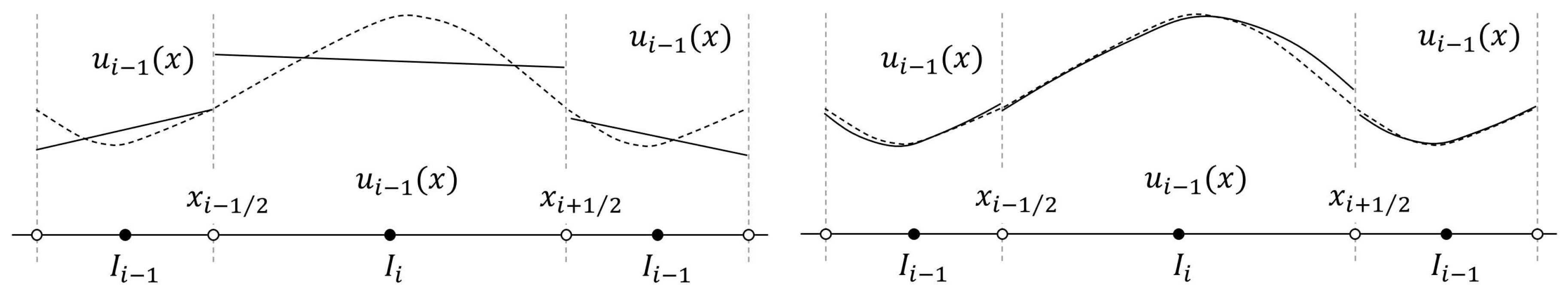
Figure 2.
Projection domain of standard actuator line model in blade (a) and advanced actuator line model in blade (b).
Figure 2.
Projection domain of standard actuator line model in blade (a) and advanced actuator line model in blade (b).
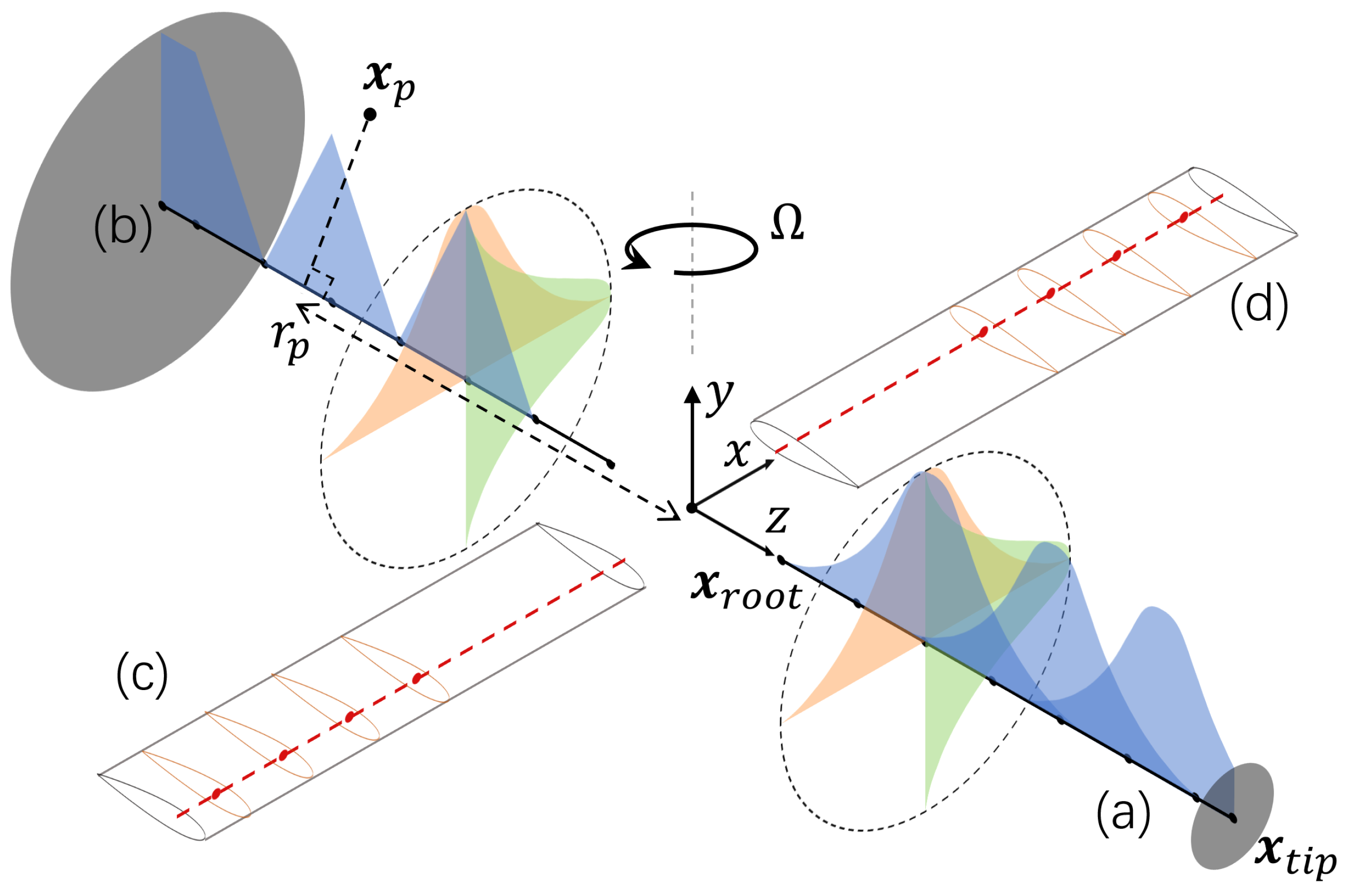
Figure 3.
Schematic diagram of a 2D blade element.
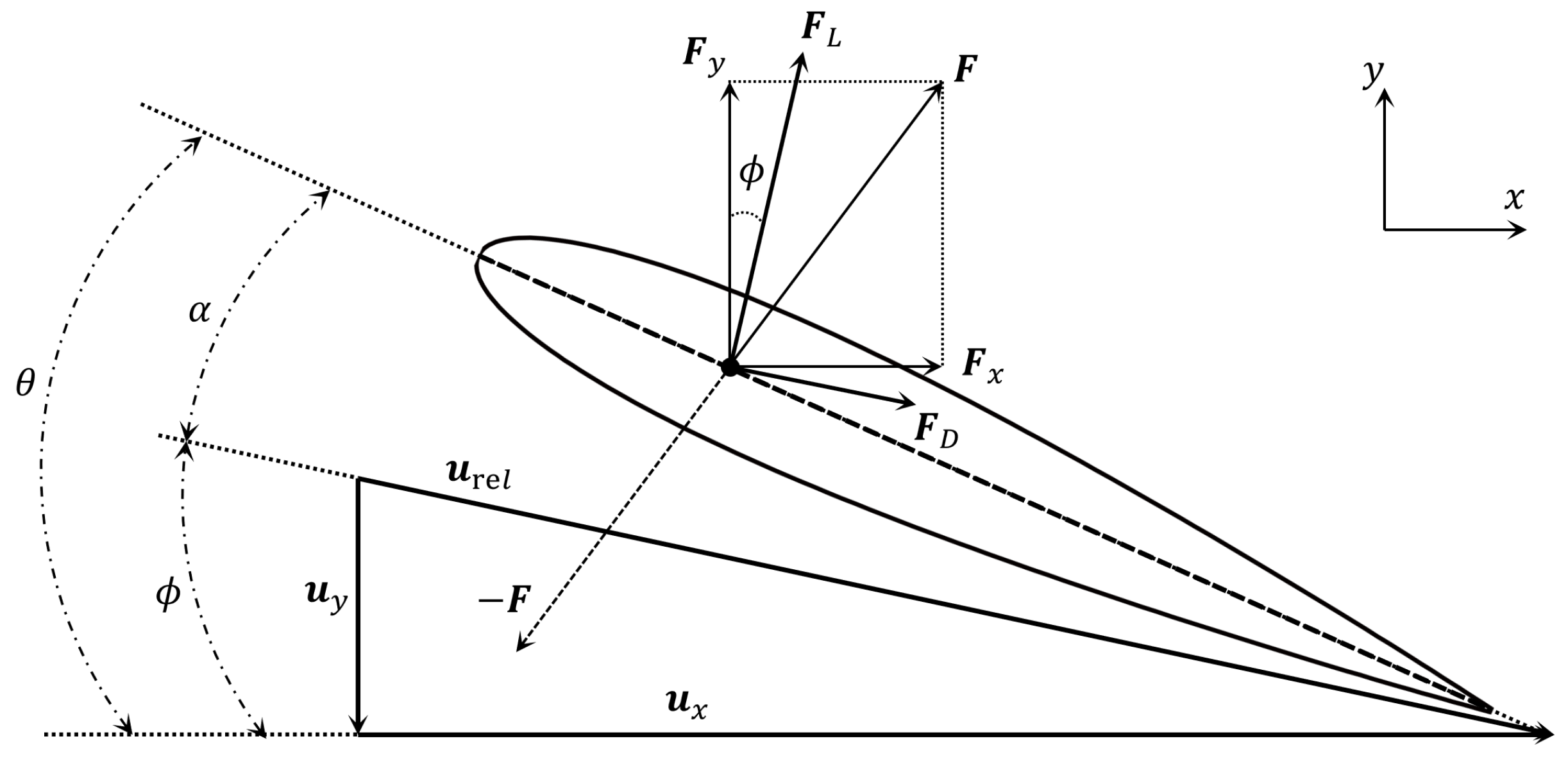
Figure 4.
Schematic diagram of the distribution of G and on a blade.
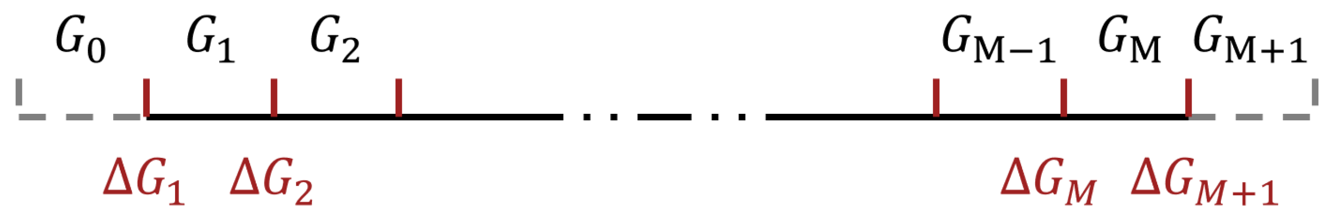
Figure 5.
The meshes used for 2D infinite wing: (a) Mesh for NACA0012 airfoil. (b) Mesh for 2D ALM.
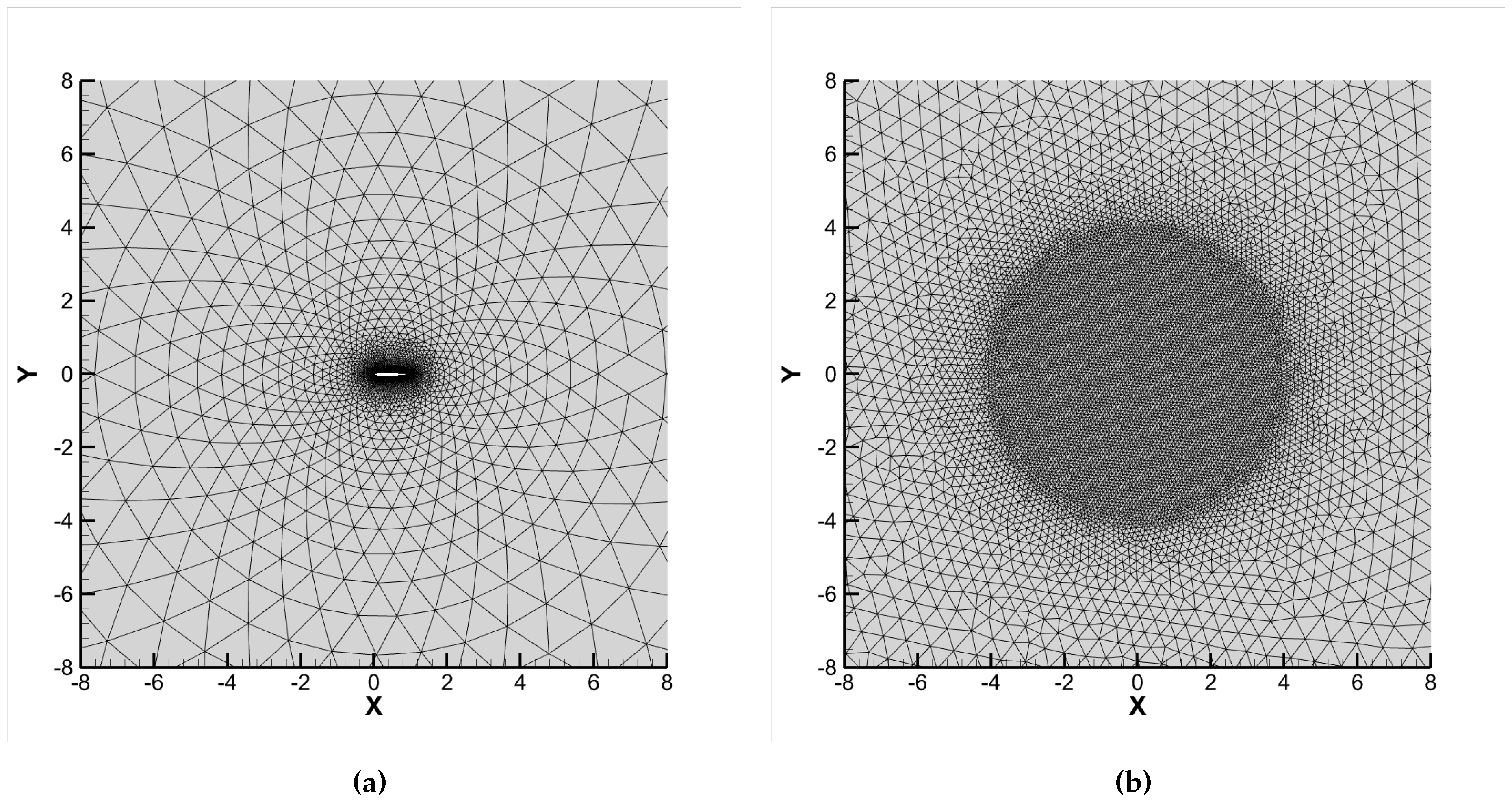
Figure 6.
Mach number contours from to : (a) Result of NACA0012 airfoil. (b) Result of ALM with . (c) Result of ALM with .
Figure 6.
Mach number contours from to : (a) Result of NACA0012 airfoil. (b) Result of ALM with . (c) Result of ALM with .
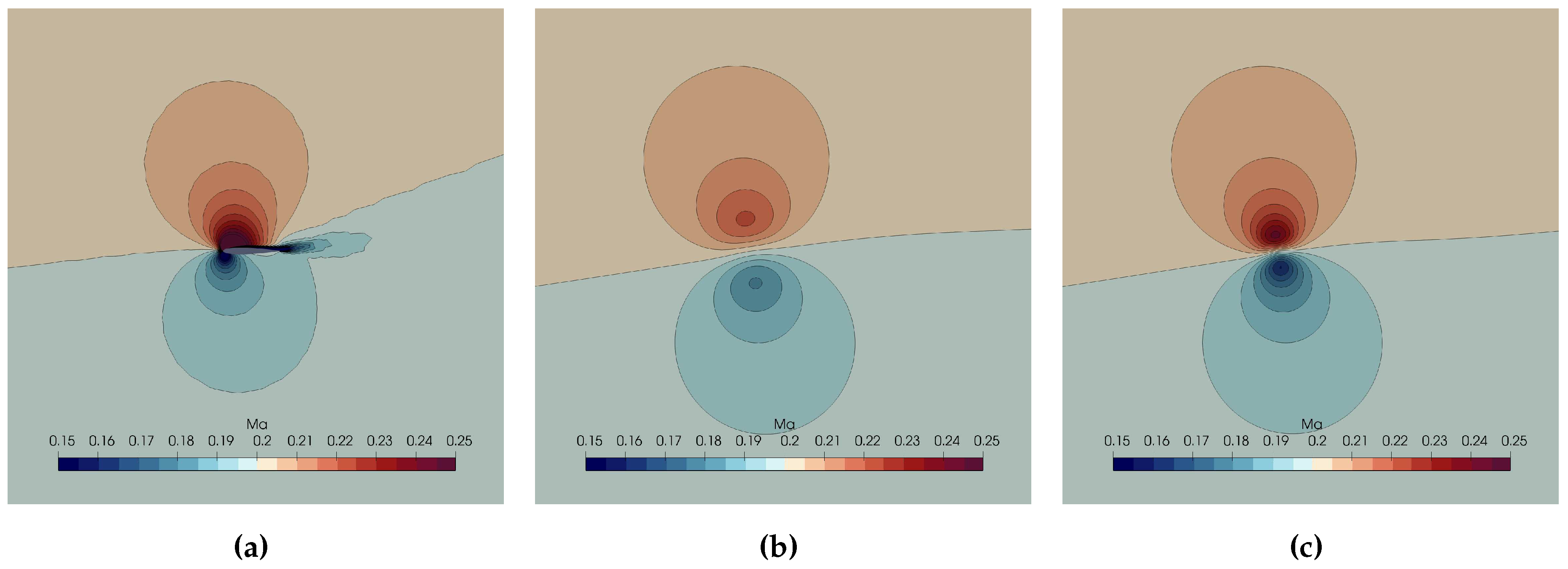
Figure 7.
Point sampling error for ALM: (a) Error of magnitude of sampled velocity for different . (b) Error of attack of angle for different . (c) Error of magnitude of sampled velocity for different . (d) Error of attack of angle for different .
Figure 7.
Point sampling error for ALM: (a) Error of magnitude of sampled velocity for different . (b) Error of attack of angle for different . (c) Error of magnitude of sampled velocity for different . (d) Error of attack of angle for different .
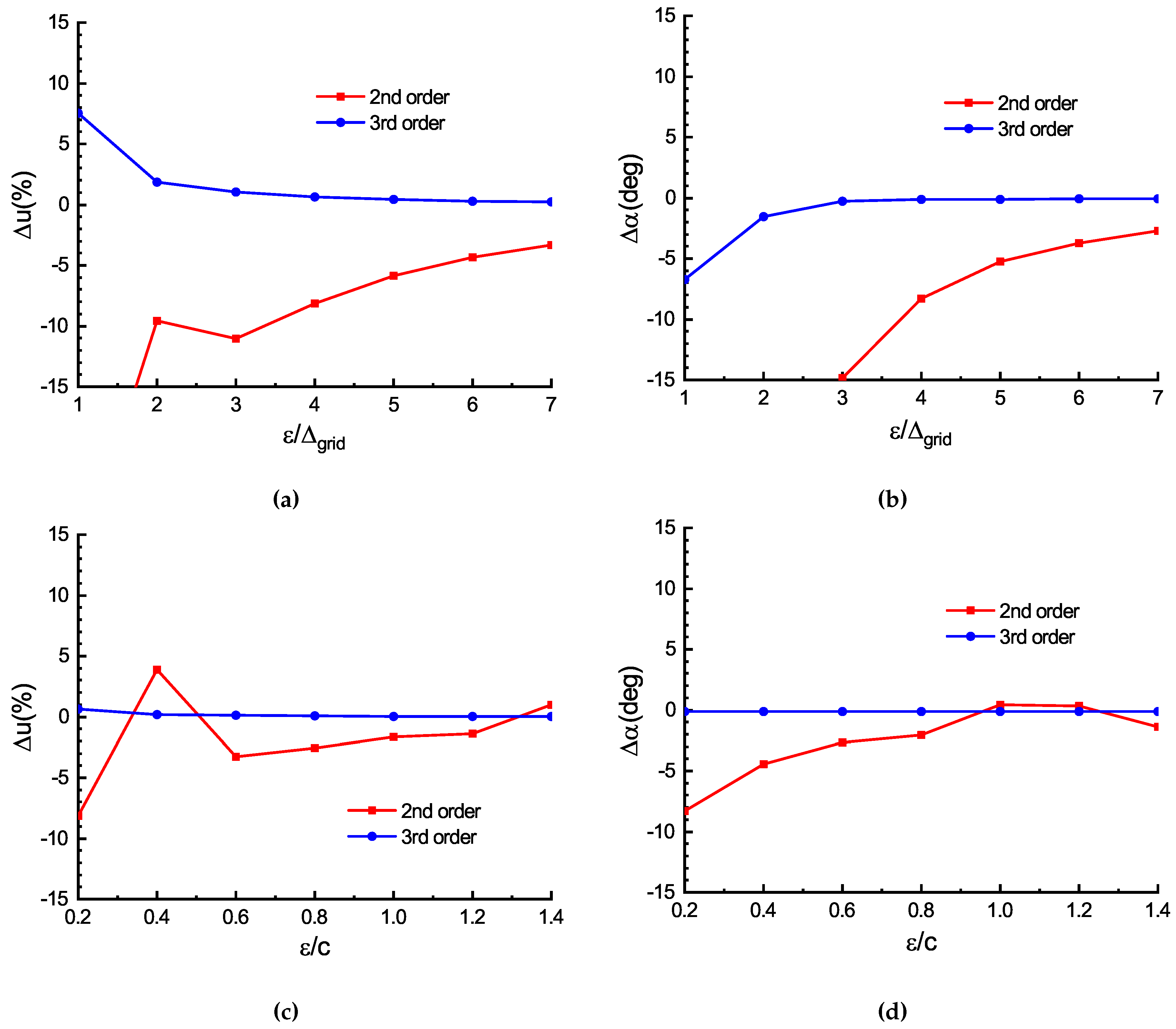
Figure 8.
Integral sampling error for ALM: (a) Error of magnitude of sampled velocity for different . (b) Error of attack of angle for different . (c) Error of magnitude of sampled velocity for different . (d) Error of attack of angle for different .
Figure 8.
Integral sampling error for ALM: (a) Error of magnitude of sampled velocity for different . (b) Error of attack of angle for different . (c) Error of magnitude of sampled velocity for different . (d) Error of attack of angle for different .
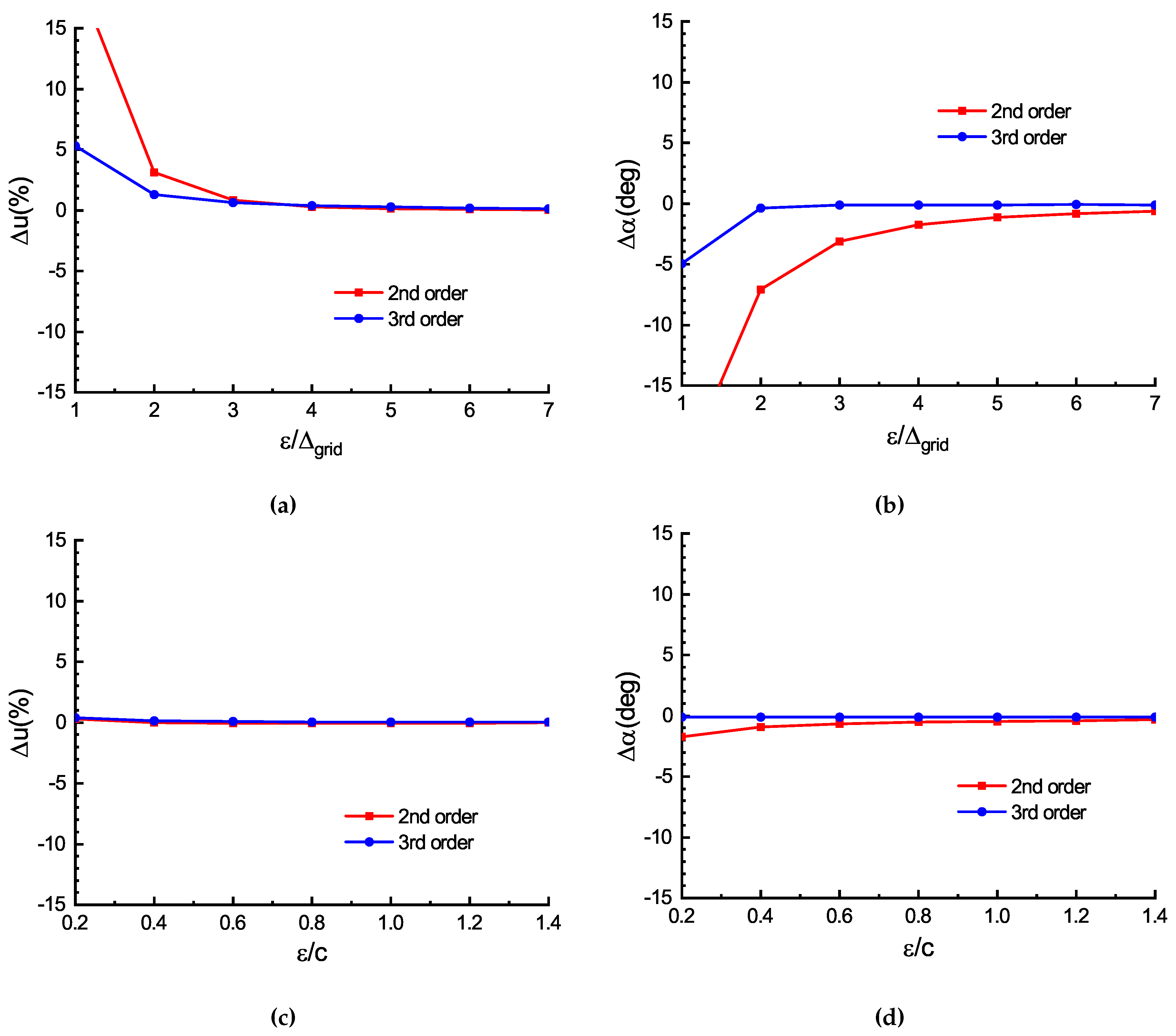
Figure 9.
Discription of the mesh for 3D finite wing and iso-surface of the Q-Criterion with of ALM simulation of constant circulation rectangular wing.
Figure 9.
Discription of the mesh for 3D finite wing and iso-surface of the Q-Criterion with of ALM simulation of constant circulation rectangular wing.
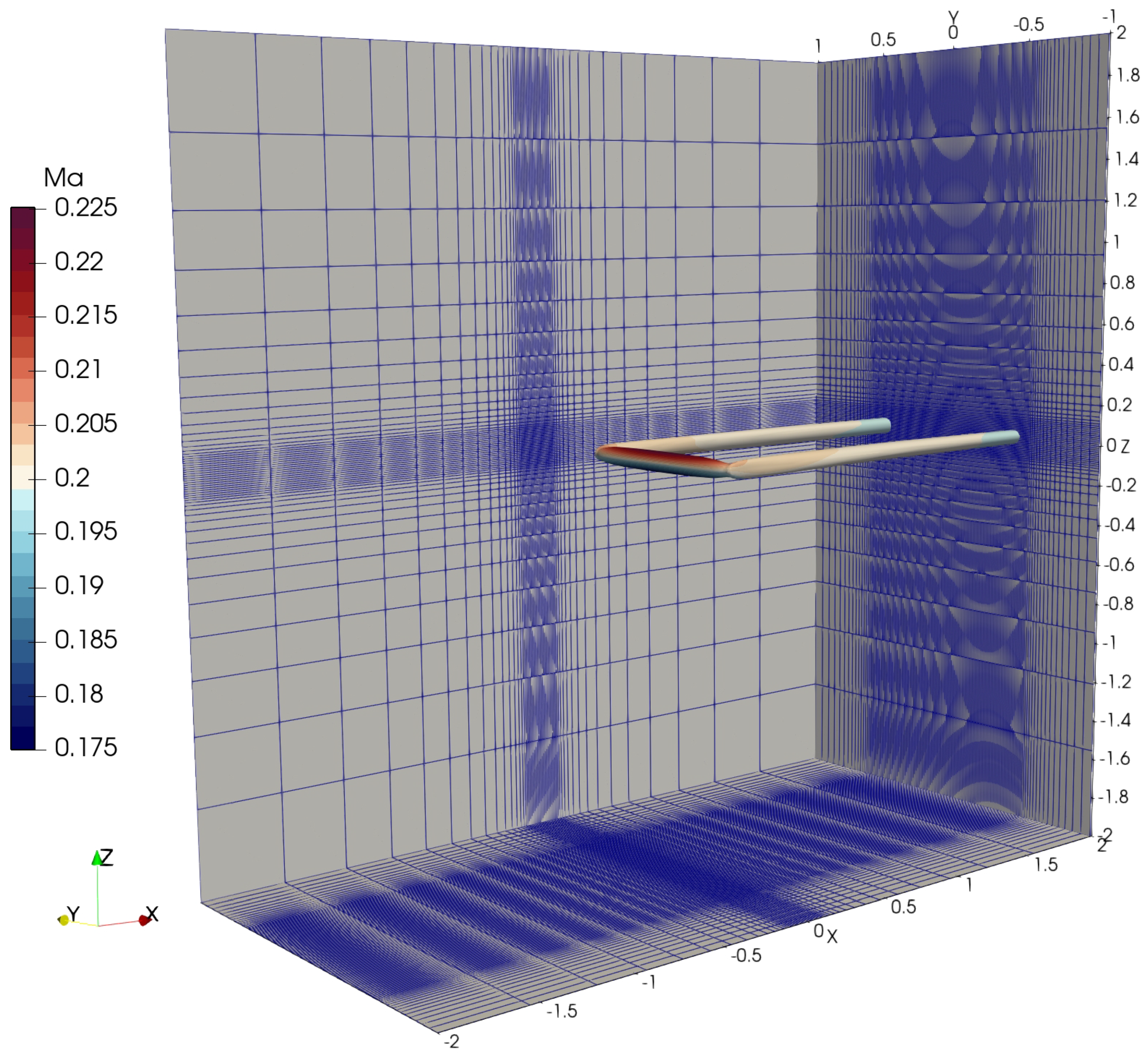
Figure 10.
Downwash distribution for solvers with different order and models: (a) ALM result of second-order solver. (b) ALM result of third-order solver.
Figure 10.
Downwash distribution for solvers with different order and models: (a) ALM result of second-order solver. (b) ALM result of third-order solver.
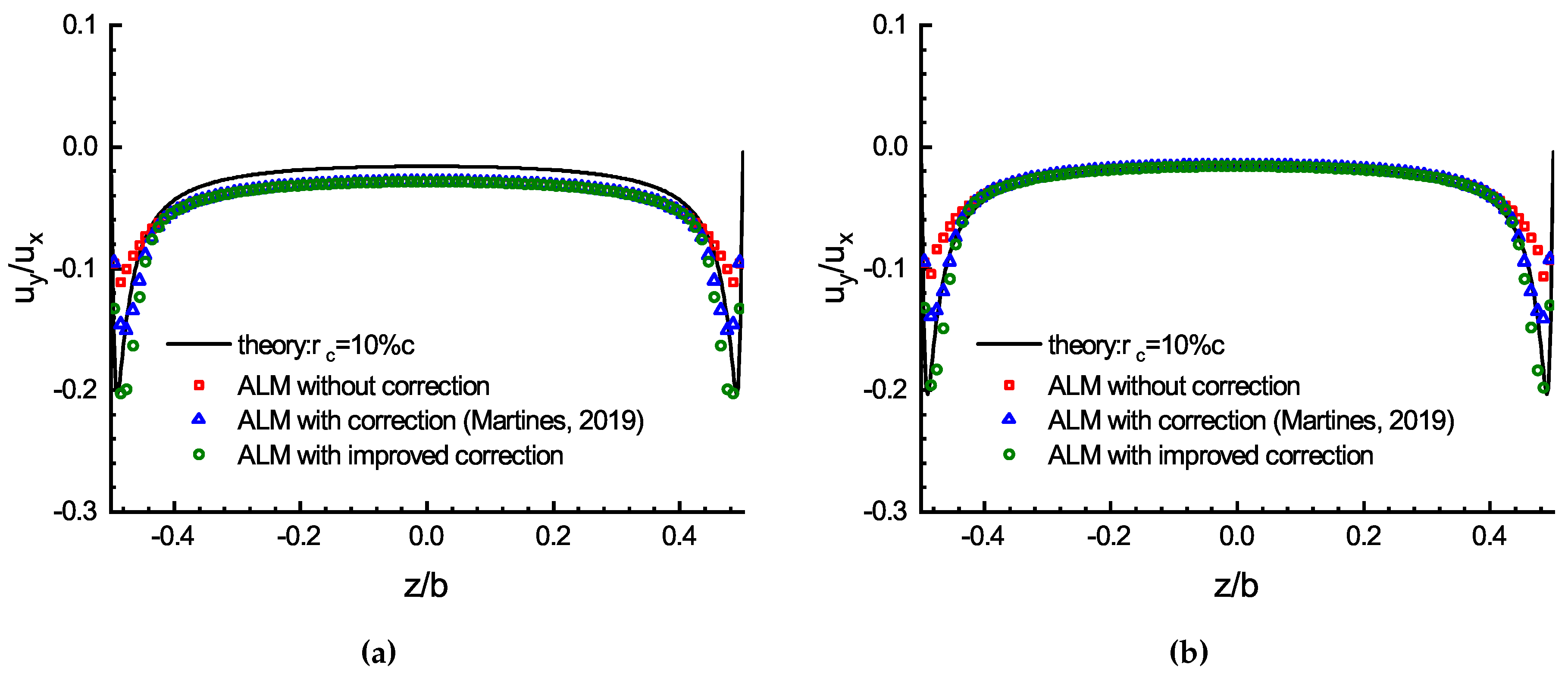
Figure 11.
Downwash distribution for solvers with different order and models: (a) ALM result of second-order solver. (b) ALM result of third-order solver.
Figure 11.
Downwash distribution for solvers with different order and models: (a) ALM result of second-order solver. (b) ALM result of third-order solver.
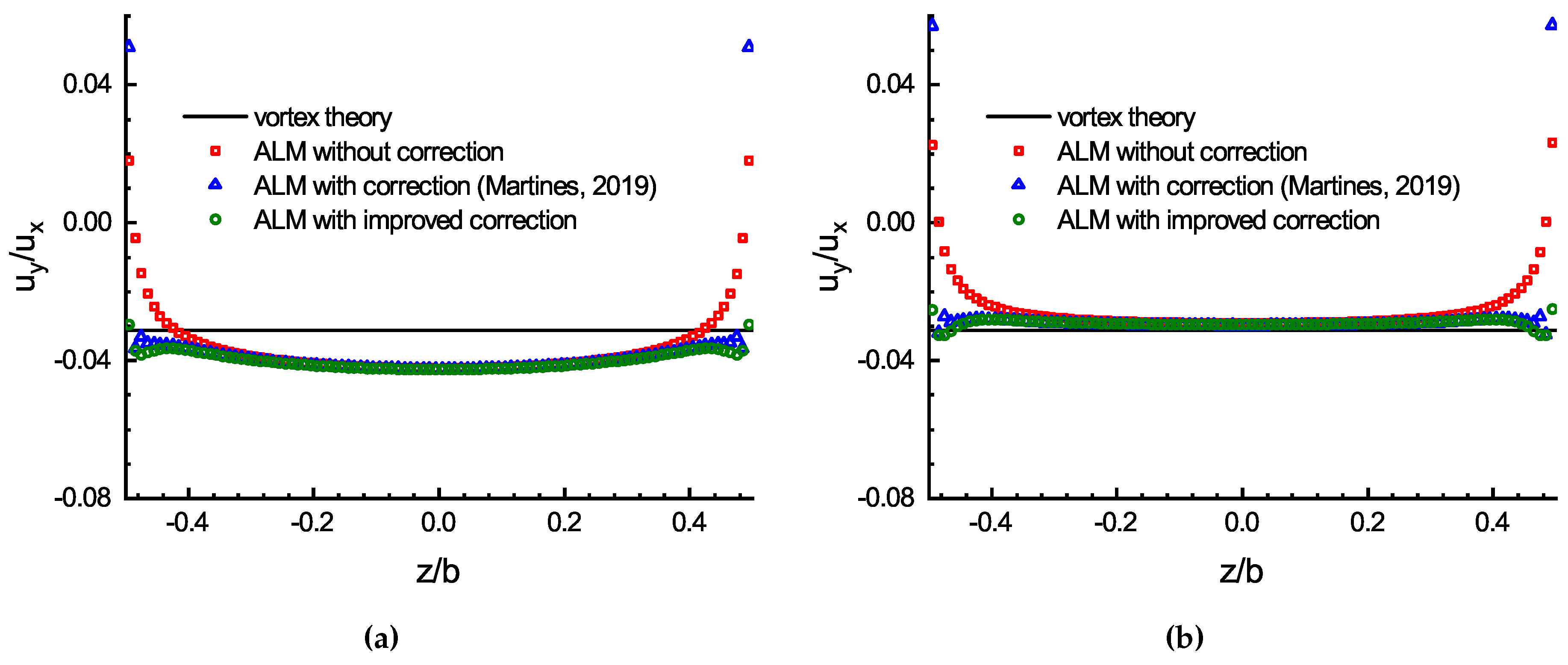
Figure 12.
The mesh used for hover flight rotor: (a) Mesh XY-plane view. (b) Mesh YZ-plane view.
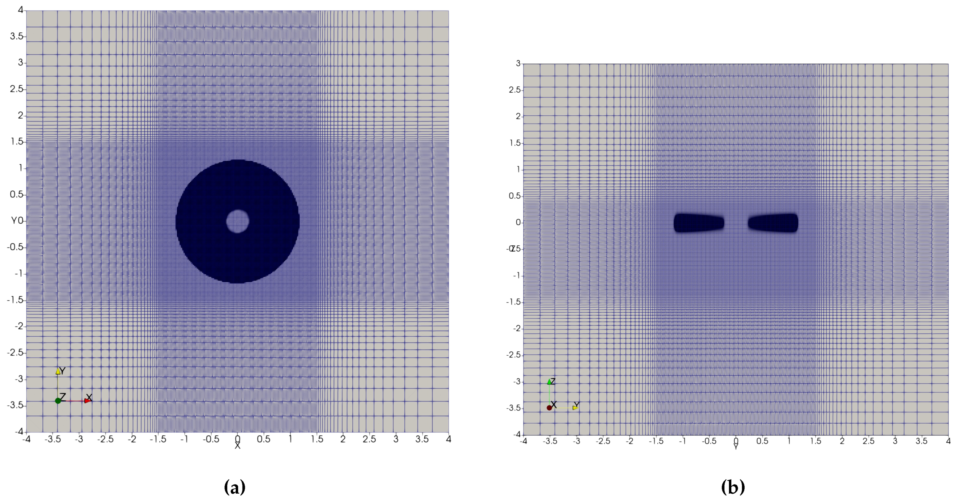
Figure 13.
Ma contours of hover flight rotor with collective pitch: (a) ADM result of the second-order solver. (b) ADM result of the third-order solver.
Figure 13.
Ma contours of hover flight rotor with collective pitch: (a) ADM result of the second-order solver. (b) ADM result of the third-order solver.
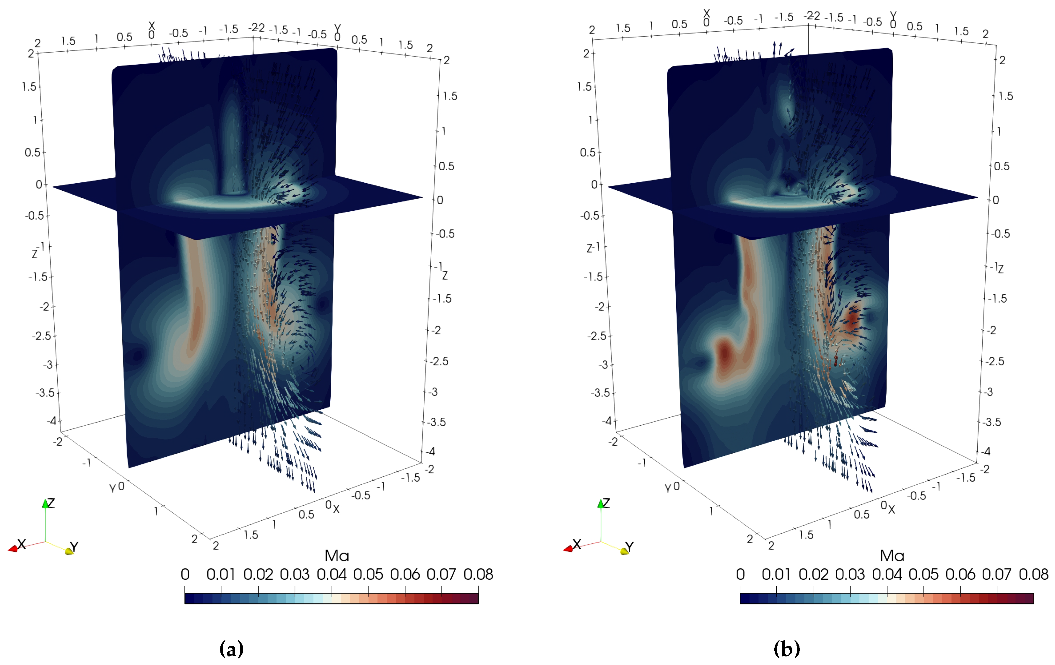
Figure 14.
Ma contours of rotor with collective pitch: (a) ADM result of the second-order solver. (b) ADM result of the third-order solver.
Figure 14.
Ma contours of rotor with collective pitch: (a) ADM result of the second-order solver. (b) ADM result of the third-order solver.
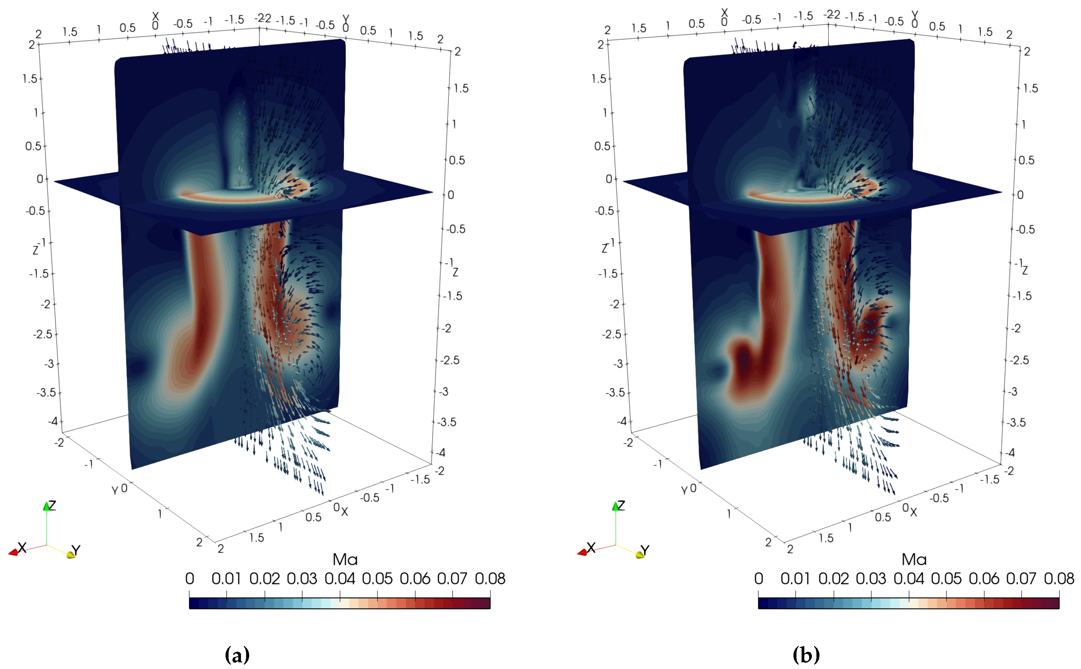
Figure 15.
Vorticity contours at iso-surface of rotor with collective pitch: (a) ALM result of the second-order solver. (b) ALM result of the third-order solver.
Figure 15.
Vorticity contours at iso-surface of rotor with collective pitch: (a) ALM result of the second-order solver. (b) ALM result of the third-order solver.
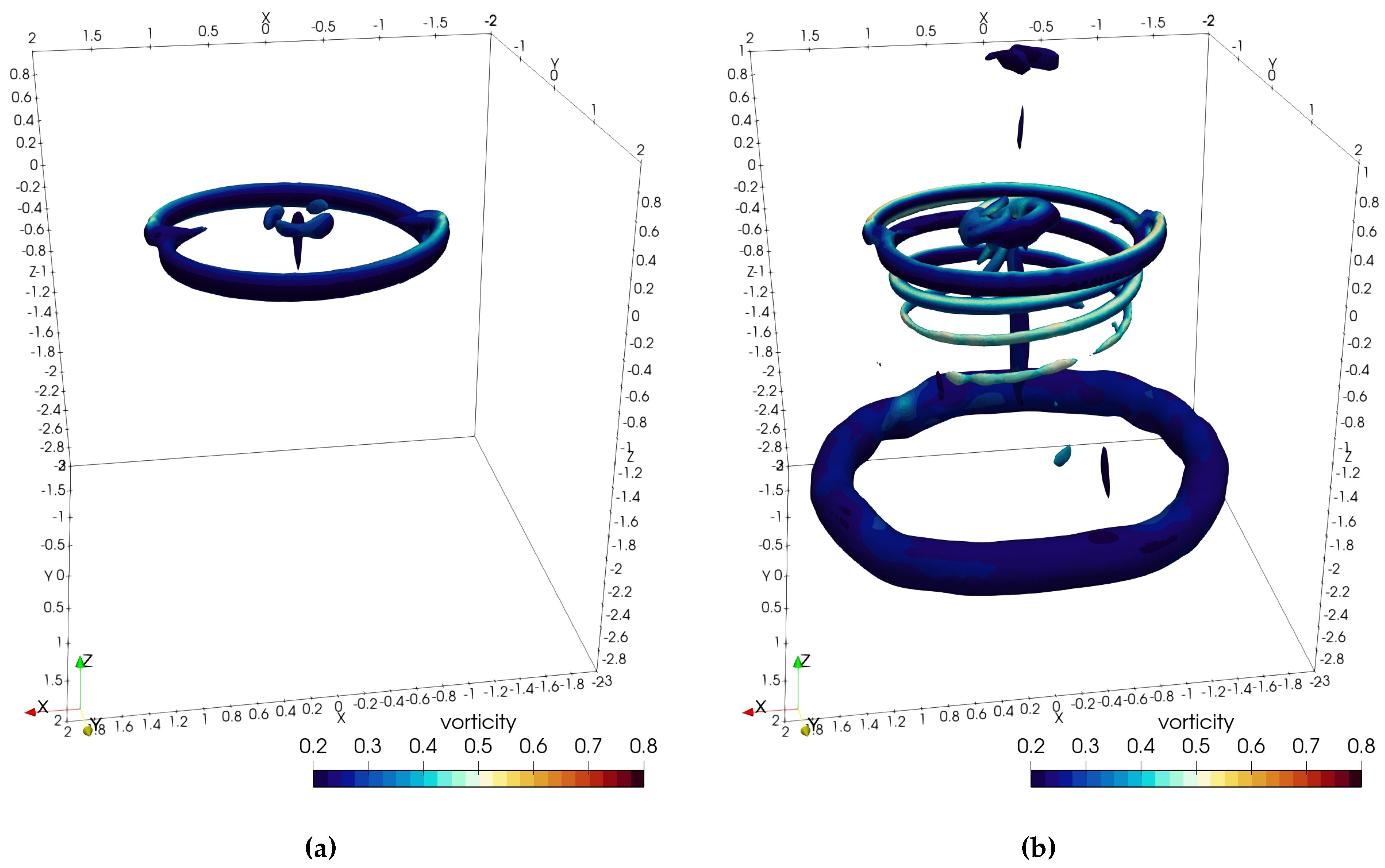
Figure 16.
Vorticity contours at iso-surface of hover flight rotor with collective pitch: (a) ALM result of the second-order solver. (b) ALM result of the third-order solver.
Figure 16.
Vorticity contours at iso-surface of hover flight rotor with collective pitch: (a) ALM result of the second-order solver. (b) ALM result of the third-order solver.
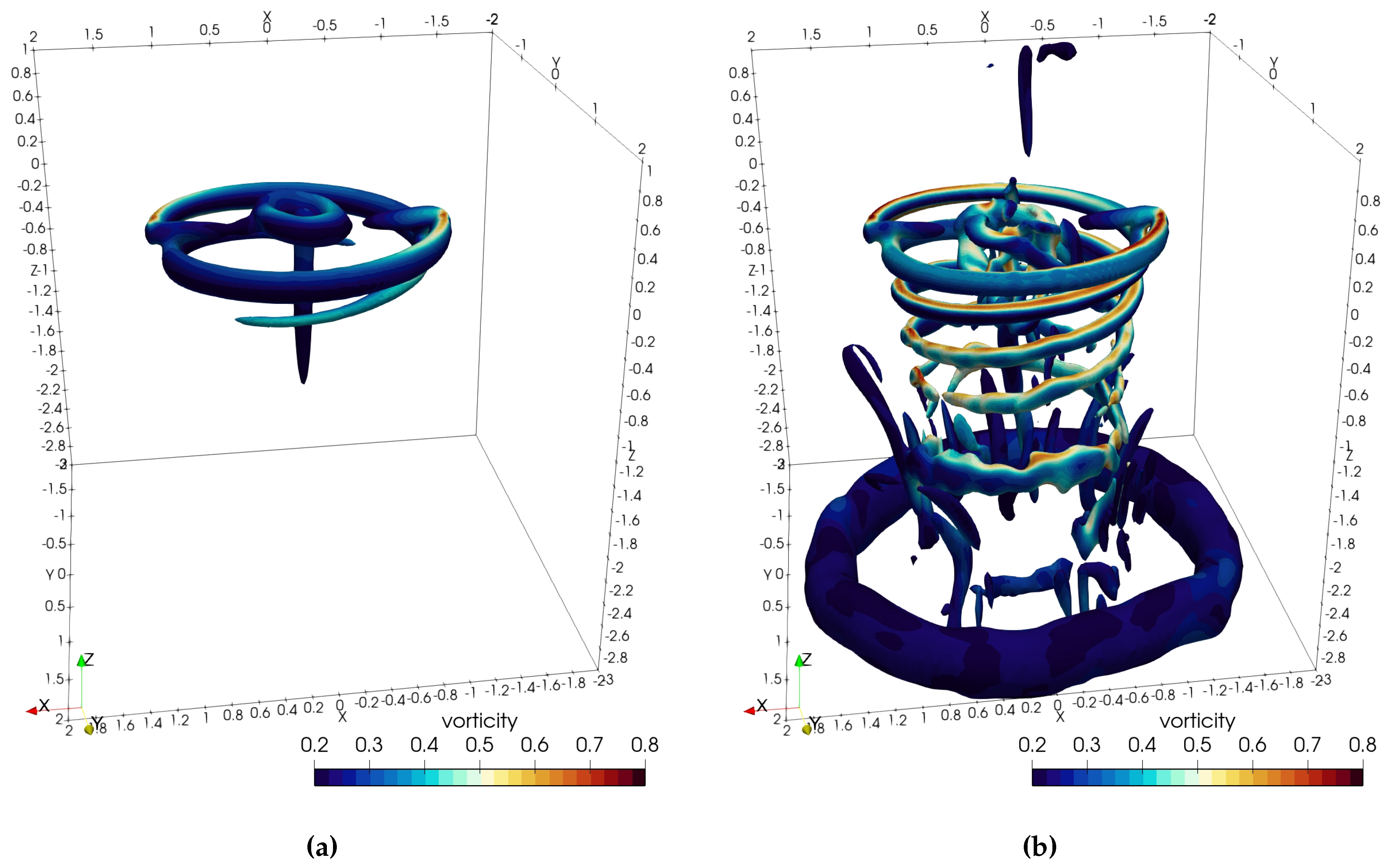
Figure 17.
Sectional life coefficients distributions of the blade: (a) Result of second-order solver with collective pitch. (b) Result of third-order solver with collective pitch. (c) Result of second-order solver with collective pitch. (d) Result of third-order solver with collective pitch.
Figure 17.
Sectional life coefficients distributions of the blade: (a) Result of second-order solver with collective pitch. (b) Result of third-order solver with collective pitch. (c) Result of second-order solver with collective pitch. (d) Result of third-order solver with collective pitch.
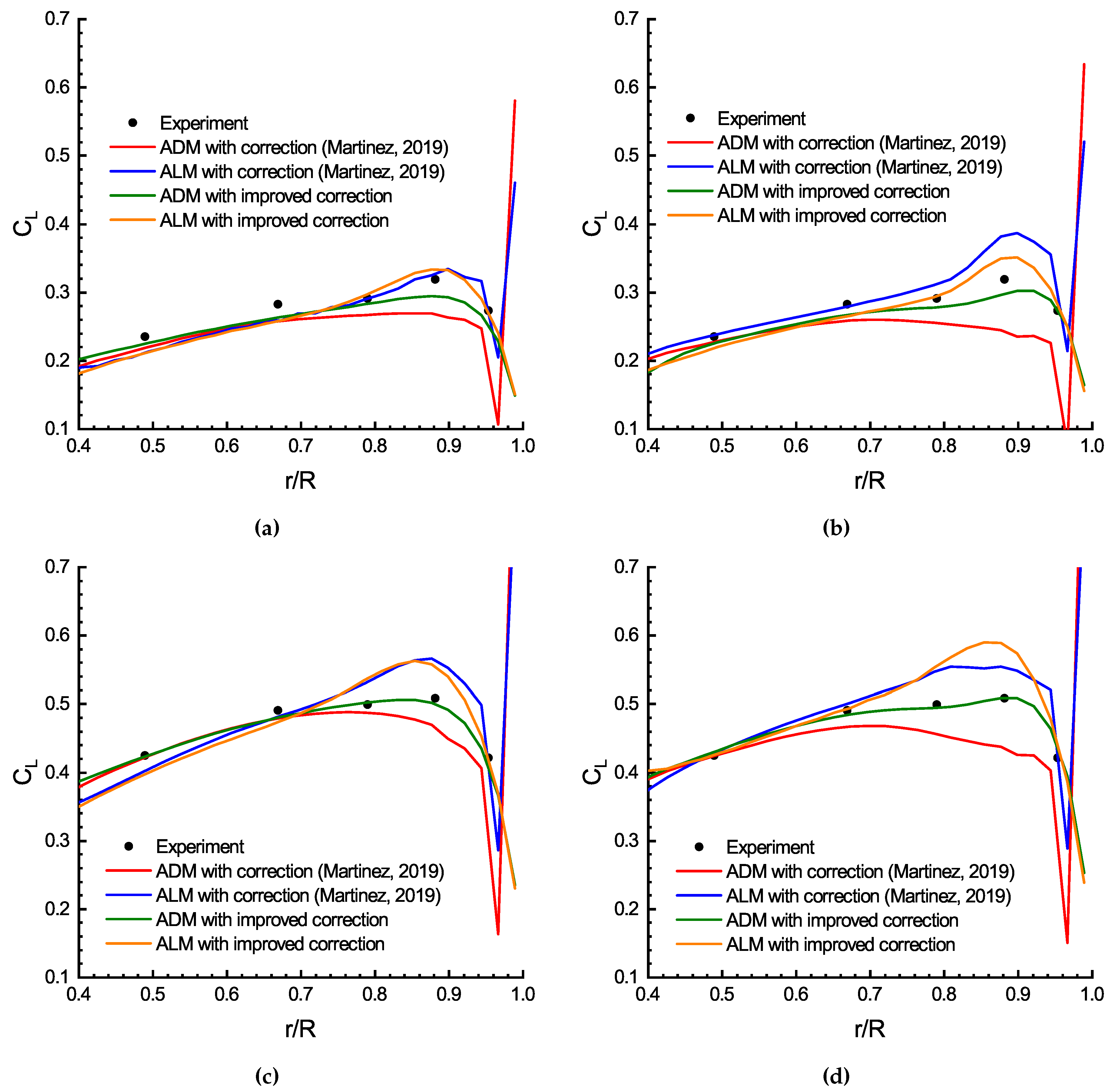
Figure 18.
Axial and radial positions of the vortex core: (a) Rotor with collective pitch. (b) Rotor with collective pitch.
Figure 18.
Axial and radial positions of the vortex core: (a) Rotor with collective pitch. (b) Rotor with collective pitch.
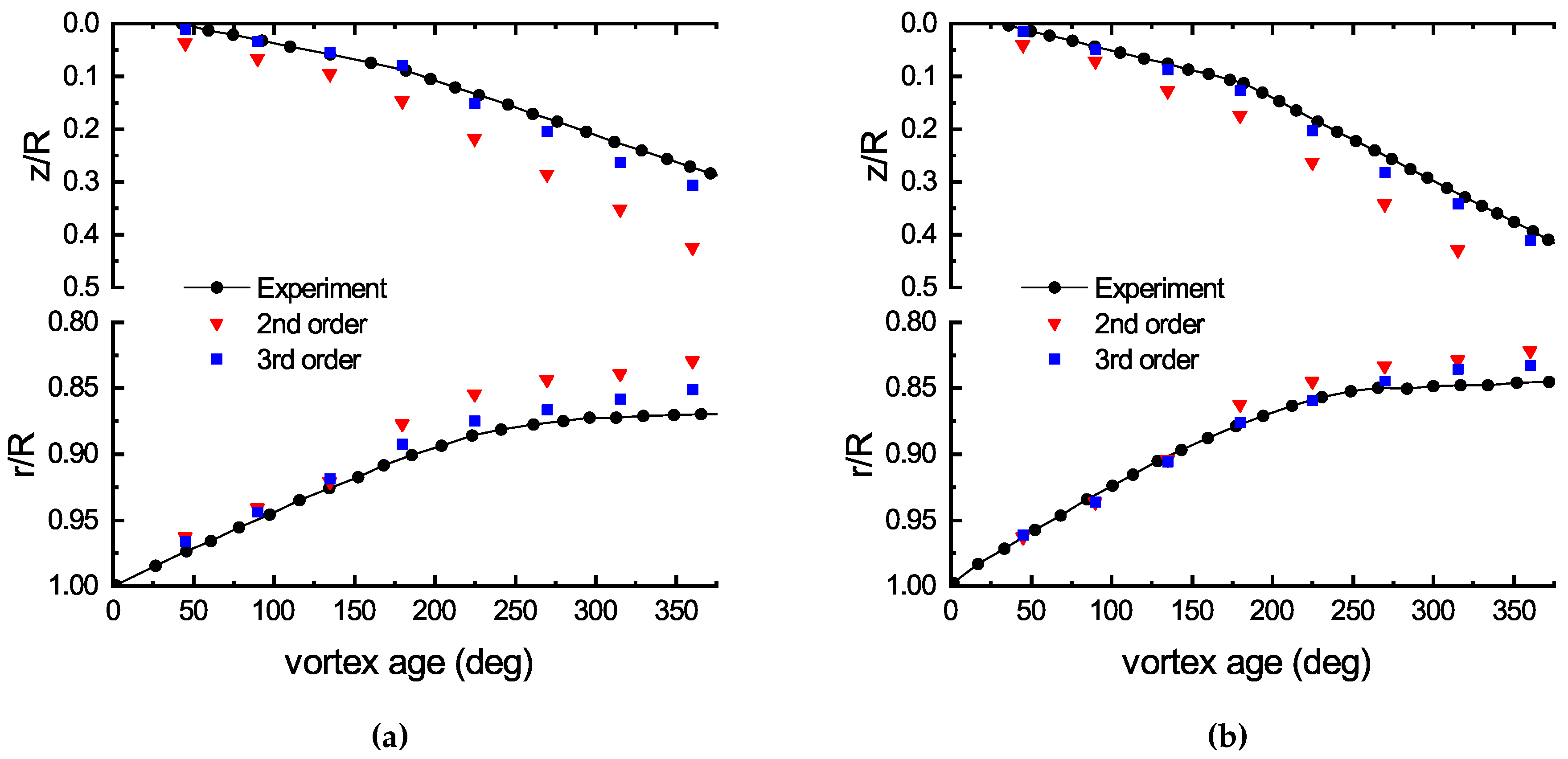
Figure 19.
Schematic diagram of the forward flight rotor.
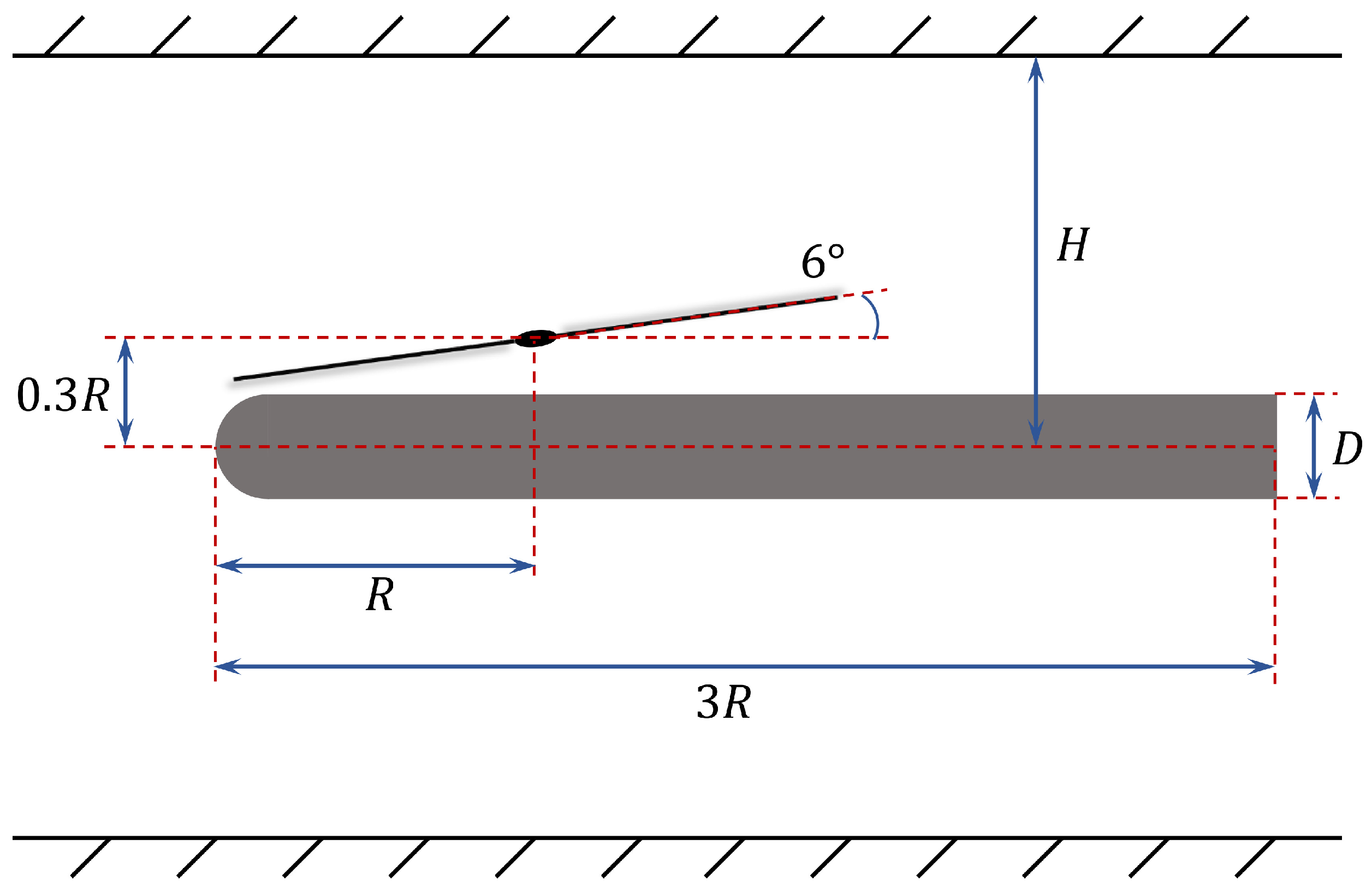
Figure 20.
The mesh used for forward flight rotor: (a) Mesh XY-plane view. (b) Mesh XZ-plane view.
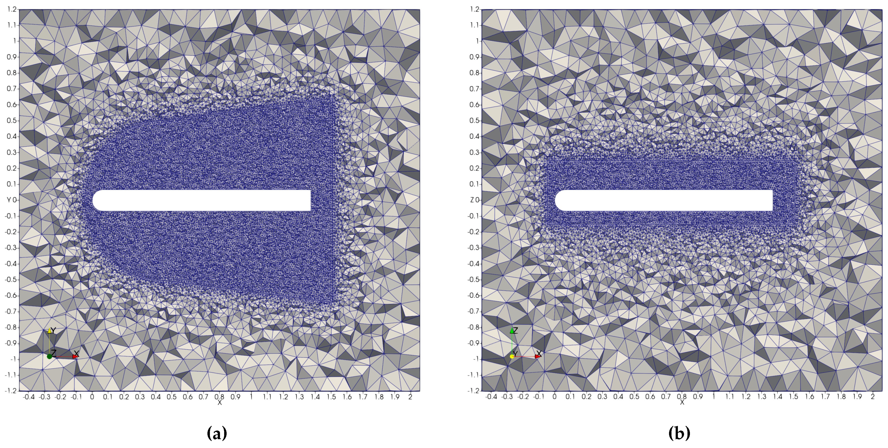
Figure 21.
Vorticity contours at iso-surface of rotor with collective pitch: (a) ALM result of the second-order solver. (b) ALM result of the third-order solver.
Figure 21.
Vorticity contours at iso-surface of rotor with collective pitch: (a) ALM result of the second-order solver. (b) ALM result of the third-order solver.
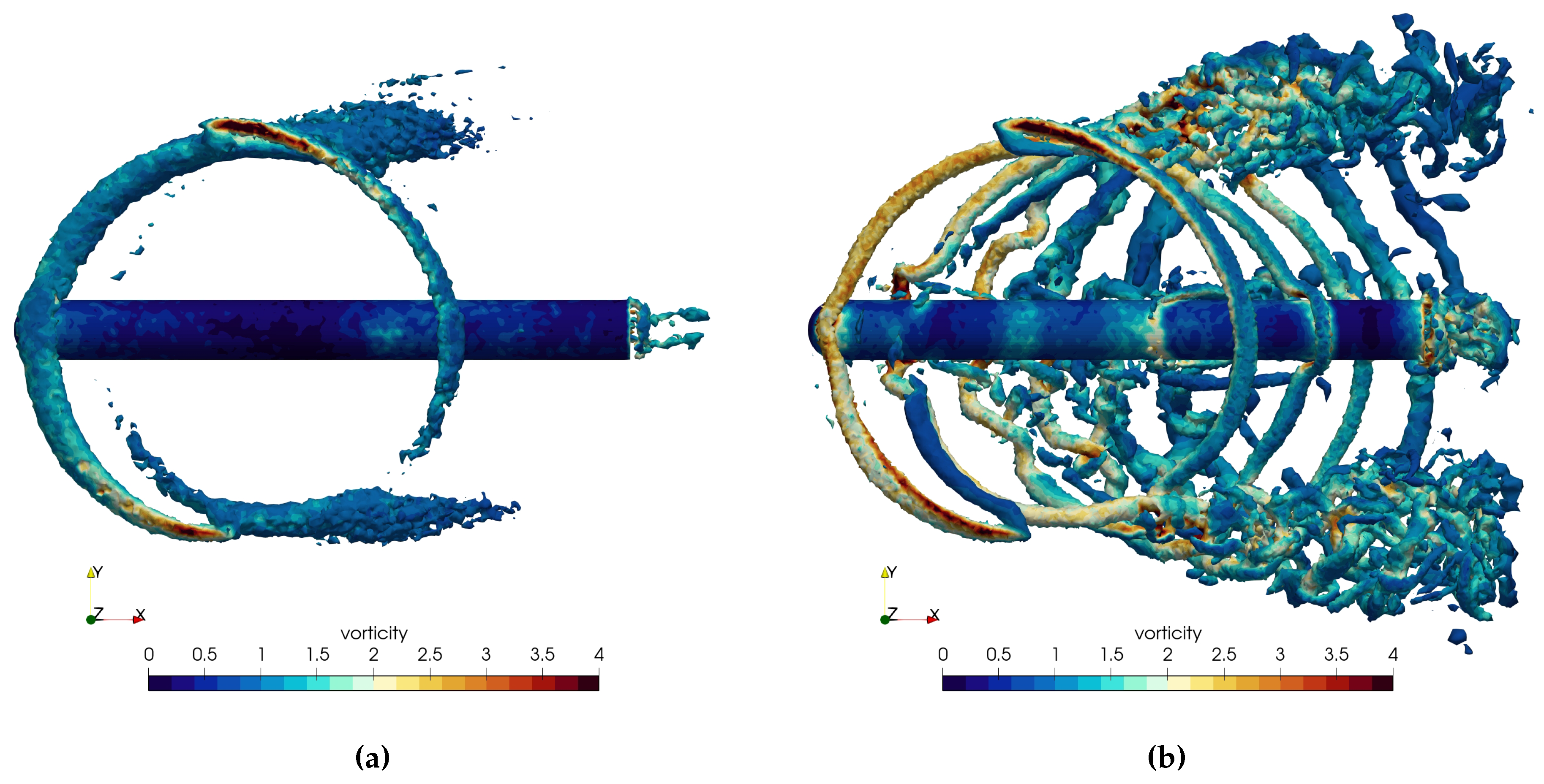
Figure 22.
Vorticity contours at iso-surface of rotor with collective pitch: (a) ALM result of the second-order solver. (b) ALM result of the third-order solver.
Figure 22.
Vorticity contours at iso-surface of rotor with collective pitch: (a) ALM result of the second-order solver. (b) ALM result of the third-order solver.
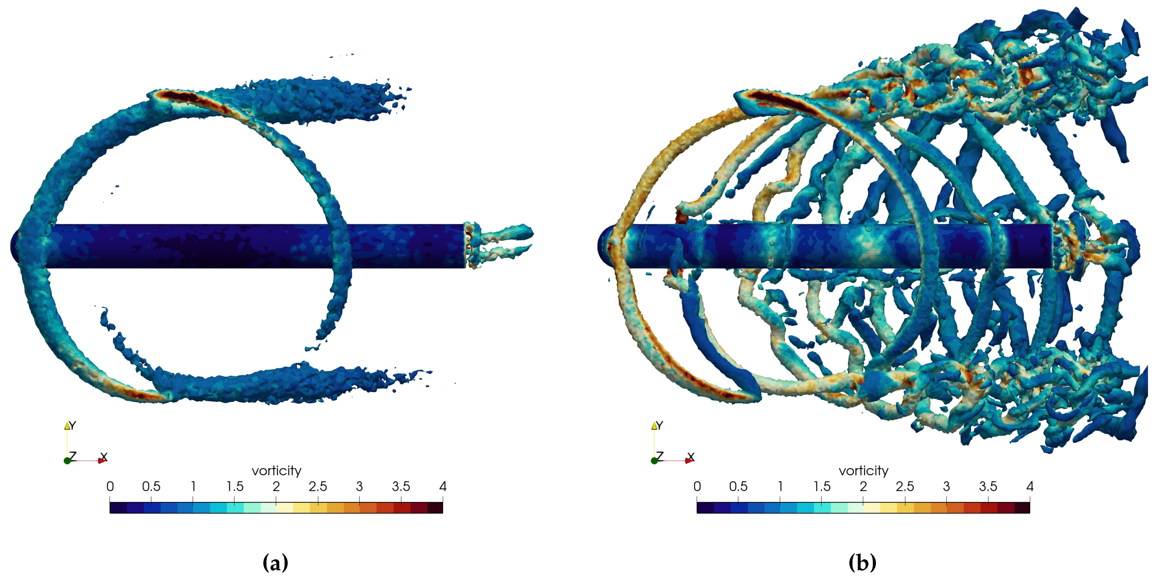
Figure 23.
Comparison between the calculated and experimental results of Cp on the top of the fuselage: (a) Result of . (b) Result of .
Figure 23.
Comparison between the calculated and experimental results of Cp on the top of the fuselage: (a) Result of . (b) Result of .
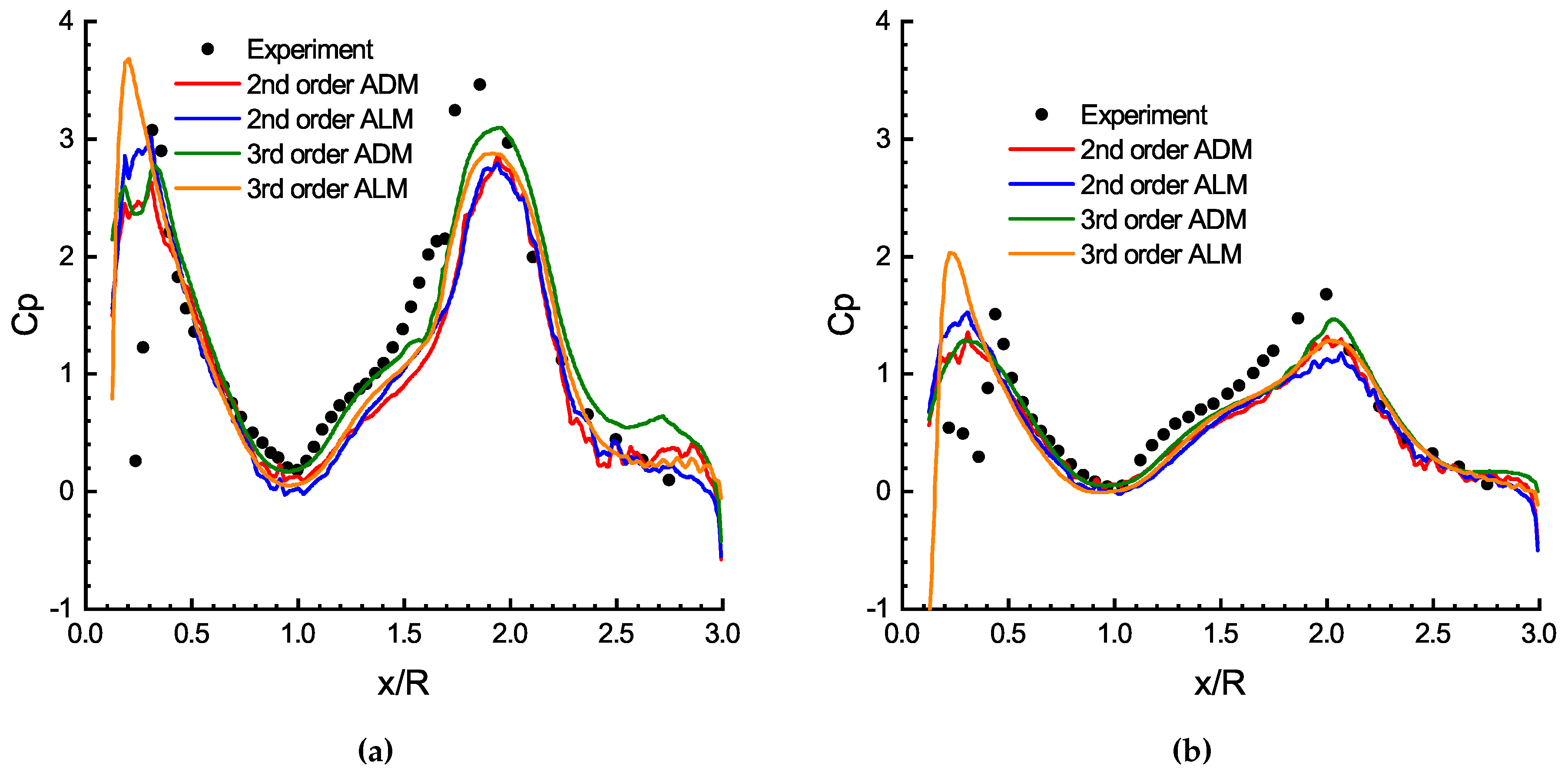
Figure 24.
Parallel scaling efficiency of the third-order solver with ALM.
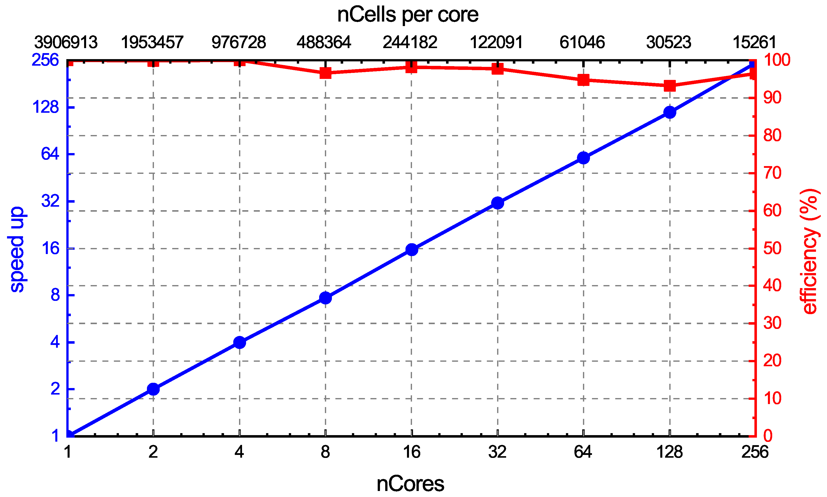

Table 1.
Performance comparison of experiment and solvers with different models with improved correction.
Table 1.
Performance comparison of experiment and solvers with different models with improved correction.
| Experiment | 2nd order ADM | 2nd order ALM | 3rd order ADM | 3rd order ALM | |
|---|---|---|---|---|---|
| , | 0.0046 | 0.004457 | 0.004595 | 0.004538 | 0.004728 |
| Error | -3.1 | -0.1 | -1.3 | 2.8 | |
| , | 0.0079 | 0.007777 | 0.007997 | 0.007951 | 0.00828 |
| Error | -1.6 | 1.2 | 0.6 | 4.7 |
Disclaimer/Publisher’s Note: The statements, opinions and data contained in all publications are solely those of the individual author(s) and contributor(s) and not of MDPI and/or the editor(s). MDPI and/or the editor(s) disclaim responsibility for any injury to people or property resulting from any ideas, methods, instructions or products referred to in the content. |
© 2023 by the authors. Licensee MDPI, Basel, Switzerland. This article is an open access article distributed under the terms and conditions of the Creative Commons Attribution (CC BY) license (http://creativecommons.org/licenses/by/4.0/).
Copyright: This open access article is published under a Creative Commons CC BY 4.0 license, which permit the free download, distribution, and reuse, provided that the author and preprint are cited in any reuse.


