
Submitted:
10 November 2023
Posted:
13 November 2023
You are already at the latest version
Abstract
The quickest path problem in the multistate flow networks, also known as the quickest path reliability problem (QPRP), aims at calculating the probability of transmitting a minimum of d units of flow/dat/commodity from a source node to a destination node through one single path within T units of time. Several exact and approximation algorithms have been proposed in the literature to address this problem. Most of the exact algorithms in the literature need prior knowledge of all the network’s minimal paths (MPs), which is considered a weak point. In addition to the time, the budget is always limited in real-world systems, making it an essential consideration in the analysis of systems’ performance. Hence, this study considers the QPRP under the cost constraints and provides an efficient approach based on the node-child matrix to address the problem without knowing the MPs. We show the correctness of the algorithm, compute its complexity results, illustrate it through a benchmark example, and conduct extensive experimental results on the known benchmarks and one thousand randomly generated test problems to demonstrate its practical superiority compared to the existing algorithms in the literature.
Keywords:
Quickest path problem
; Network reliability
; Multistate flow networks
; Minimal paths
; Algorithms
1. Introduction
The quickest path problem involves identifying a path from a source node, 1, to a destination node, n, within a network. This path is used to efficiently transmit a specific flow quantity, d, from node 1 to node n while minimizing the transmission time [1,2]. In this problem, each network arc is characterized by two key attributes: a lead time value and a capacity value. The significance of this optimization problem is well-recognized by researchers due to its applicability across a broad spectrum of flow network scenarios [1,2,3,4,5,6,7,8,9,10,11]. This problem initially emerged in discovering the fastest route for convoy-type traffic within flow-rate-constrained networks [1]. Subsequently, it found application in communication networks, where nodes represent transmitters/receivers and arcs symbolize communication channels [2].
While deterministic (non-stochastic) flow networks have undeniably been instrumental in understanding and optimizing various systems, the practical reality is that many real-world systems exhibit dynamic characteristics, necessitating the adoption of a more nuanced approach. Multistate (stochastic) flow networks (MFNs) have gained prominence as a result of their ability to model complex systems where fluctuations, failures, maintenance, and other dynamic factors play a significant role [12,13,14,15,16,17,18,19,20]. Within an MFN, arcs and nodes can exist in various potential states, influenced by traffic conditions, maintenance activities, failures, or other underlying causes. Consequently, the network itself assumes multiple states, each reflecting the dynamic nature of the system. Numerous performance metrics have been introduced in the literature to evaluate the effectiveness of an MFN, with particular emphasis on network reliability, which stands out as a primary indicator. Network reliability is commonly defined as the system’s capacity to fulfill a predefined function within specified conditions and over a known time frame [21]. A well-known reliability indicator is the two-terminal reliability of an MFN. It is the probability of transmitting at least a given demand d units of flow/data/commodity from node 1 (source) to node n (destination). Numerous exact and approximation algorithms have been proposed in the literature to compute this indicator [8,13,22,23,24,25,26,27,28,29,30,31,32,33,34,35].
Due to the inherent random variability in arc capacities within MFNs, the transmission time likewise exhibits stochastic behavior. In light of this uncertainty, the classical quickest path problem has evolved into a more comprehensive challenge known as the quickest path reliability problem (QPRP) within the context of MFNs [4,5,27,36,37,38,39,40]. The primary objective of the QPRP is to ascertain the probability of successfully transmitting a minimum of d units of flow from source node 1 to the destination node n via a single path, all while adhering to a stipulated time constraint of T units. This extension of the problem accounts for the dynamic and unpredictable nature of network conditions, making it particularly relevant in scenarios where both speed and reliability are paramount, such as in telecommunications, transportation, and various other domains [4,27,36,41,42].
Lin [36] introduced an algorithm requiring all the MPs as input. It determines the minimum capacity required for each MP to meet the time constraints for transmitting d flow units. Subsequently, by systematically evaluating each MP, the algorithm derives the solutions to the problem. Yeh et al. [41] harnessed the kth shortest path approach to devise an algorithm for addressing the problem. In subsequent work [42], they further refined and enhanced their algorithm. The QPRP was expanded to encompass scenarios involving two disjoint MPs in [38,43], as well as situations with multiple disjoint MPs in [38]. In a different approach, the researchers in [40] considered both time and budget constraints, utilizing these constraints to reduce computational complexity efficiently. Their extensive numerical analysis underscored the effectiveness of the proposed algorithm. This work was subsequently improved upon in [44]. Furthermore, researchers in [5] recognized the computational limitations of the algorithm presented in [36], mainly when the network configuration involves over thirty relevant MPs. To address this challenge, they introduced an unbiased Monte Carlo estimator as an alternative to exact evaluation, offering a more scalable solution for large-scale scenarios. In a recent development, detailed in [4], the authors addressed integrating budget constraints into the QPRP. They introduced an innovative approach that capitalizes on budget and time constraints to streamline the process by eliminating redundant MPs before algorithm execution. The authors then conducted extensive numerical experiments to underscore the enhanced performance of their approach when compared to existing methods in the literature. However, their algorithm still needs all the MPs as input.
Recognizing the inherent computational challenge of determining all MPs, which is an hard, this study introduces an efficient approach designed to address the QPRP under the cost constraints, all without prior knowledge of MPs. Based on the node-child matrix, our proposed algorithm offers a novel methodology for solving the problem. To underscore its efficiency, we provide complexity analyses and present a wealth of experimental results, establishing the algorithm’s superior performance compared to existing methods in the literature.
The subsequent sections of this paper are organized as follows. Section 2 states the required notations, nomenclature, and assumptions. Section 3 provides some preliminaries on the problem. The proposed algorithm is stated in Section 4. The complexity results and an illustrative example are given in Section 5. We conduct several experimental results on benchmarks and randomly generated test problems in Section 6. Finally, we conclude the work in Section 7.
2. Notations, nomenclature, and assumptions
|
|
|
|
|
|
|
|
|
|
|
|
|
|
|
|
|
|
|
|
|
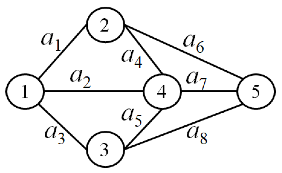
Figure 1.
A benchmark network example.
2.1. Nomenclature
- Vector X = (x1, x2, ⋯, xm) is considered less than or equal to vector Y = (y1, y2, ⋯ , ym), denoted as X ≤ Y, if xi ≤ yi holds for all i = 1, 2, ⋯ , m. If, in addition to X ≤ Y, there exists at least one j such that xj < yj, we express it as X < Y. For instance, if we take X = (4, 2, 1), Y = (3, 1, 1), and Z = (2, 2, 2), we can observe that Y < X, Z ≮ X, X ≮ Z, Y ≮ Z, and Z ≮ Y.
- We define a vector X ∊ Ψ as a minimal vector when there is no other Y ∊ Ψ such that Y < X. For example, every vector in the set {(4, 3, 1), (2, 1, 3), (3, 4, 1), (1, 2, 2)} is a minimal vector. It is worth noting that a vector does not need to be less than or equal to all other vectors in the set to be considered minimal
- Noting that a path is a set of adjacent arcs enabling data transmission from source node 1 to destination node n, we say path P1 is a subset of path P2, denoted by P1 ⊂ P2 when P2 encompasses all the arcs present in path P1.
2.2. Assumptions
- The capacity of each arc is a random integer ranging from 0 to for , following a predefined probability distribution function. It is important to emphasize that is a known integer value, representing the maximum capacity of arc .
- The arcs’ capacities are statistically independent.
- The network adheres to the flow conservation law, which means that no other node generates or accumulates flow apart from the source and destination nodes.
- All the required flow is sent through a solitary path from node 1 to node n.
- Each node is perfectly reliable.
It is worth highlighting that in cases where an unreliable node exists within the network, it can be represented as a pair of reliable nodes connected by an arc [45]. As a result, the final assumption does not impose any artificial constraints on the problem.
3. Background
We have two constraints in the problem: the budget and the time constraints, and we are looking to calculate the probability of successfully transmitting at least d units of flow from node 1 to node n such that the constraints are satisfied. One notes that the cost for transmitting d units of flow through a minimal path (MP) under system state vector (SSV) X is equal to
provided that . In fact, as we are considering the time parameter, as far as the capacity of the MP is nonzero, its amount does not play any role in computing the transmission cost. However, the capacity of an MP directly affects the transmission time.
To illustrate it, consider the network of Figure 1 with current SSV, 3, 2, 3, 4, 3, 3, 3, 5) and lead time vector 3, 1, 2, 3, 4, 3, 2, 3). Consider the scenario where we aim to transmit a flow of units from node 1 to node n through path . Observing that 3, 4, 3, 5, it is feasible, and the transmission cost is calculated as 21. Additionally, we find that 13. Since 3, the transmitted flow is limited to 3 units of flow at a time, and since 13, no flow can arrive at node n during the first 13 time units. Following this initial period, the flow is steadily pumped through, three units at a time, until the entire units of flow have successfully traversed path . Consequently, it takes a total of 13 + =16 time units to send units of flow from node 1 to node n through . Generally, the required time to transmit d units of flow from node 1 to node n through MP under SSV, X,, provided that , is equal to
where is the smallest integer number not less than x. One notes that if , it is impossible to transmit any flow through , and one can define for such a case.
To compute the reliability, one needs to find all the SSVs under which d units of flow can be sent through the network within the time T and budget b. The following result from [4] shows that it is sufficient to determine at least the minimal vectors with this property and not all of them.
Lemma 1.
[4] Assume that X and Y are two SSVs for the network G. If , then for any MP with , we have .
We now define the following function to take care of the time and budget limits simultaneously.
This way, signifies that one can transmit at least d units of flow from node 1 to node n through some MP in the network while adhering to the time and budget constraints. To elaborate, assuming , it is evident that . Moving forward, let
represent the collection of minimal vectors within , and define for . By forming sets , , , it becomes apparent that . As a result, the computation of reliability, denoted as , can be determined using the sum of disjoint products [46,47,48] as follows.
where , and . Therefore, the essential task is to determine the set .
Definition 1.
A system state vector X is called a ()- candidate if there exists an MP such that , , and .
Proposition 1.
The set is the set of all the ()- candidates.
Definition 2.
A system state vector X is a ()-, if and only if it is a ()- candidate and any is not a ()- candidate.
Proposition 2.
The set is the set of all the (real) ()-s.
In the next section, we provide an efficient algorithm to search for all the ()-s.
4. The NCM-based algorithm
As all the flow must pass through a single MP, and no MP is a subset of another MP, it is possible to determine the minimum required capacity for each MP to facilitate the transmission of d units of flow within T units of time. Let be a designated MP with . Now, if one creates an SSV, X, by setting the capacity of all the arcs within to an arbitrary positive value and the capacity of all other arcs to zero, several observations can be made: (1) The capacity of under X is , that is, . (2) The vector X is the minimal SSV under which the capacity of equals . (3) The capacity of all other MPs under X is zero, as each of them contains at least one arc not belonging to .
Hence, one needs to determine the value for such that d units of flow can be transmitted through it within T units of time. From Eq. (2), one sees that the required time to transmit d units of flow through under an arbitrary SSV, X, is equal to . Assume that . As d and are positive numbers, then , and thus should be less than T. Now, for the MP, , that satisfies and , we have
As a result, is the minimum possible capacity for such that d units of time can be transmitted through it within T units of time. If , it is possible to create the corresponding SSV, X, described above, which is the corresponding ()- to . Otherwise, it is impossible to have such a ()-.
This forms the fundamental concept behind several algorithms presented in the literature, which rely on having access to all the MPs and inspecting each one individually to assess the feasibility of conducting the necessary transmission [4,36]. Nonetheless, the primary drawback of such algorithms lies in their dependence on the complete set of MPs. It is noteworthy that determining all the MPs is intrinsically an -hard problem, as established in [37,49]. Here, we use the idea of the node-child matrix utilized in [50] to propose an efficient algorithm that does not need any MP in advance.
The node-child matrix of an MFN is structured as an matrix, where q represents the maximum out-degree of all the nodes within the network, determined as . In this matrix, each row corresponds to a specific node in the network and indicates its child nodes. For instance, the following is the node-child matrix related to the network depicted in Figure 1.
One notes that the out-degrees of different nodes in the network may not be uniform. Consequently, when the out-degree of a specific node is less than the maximum out-degree q, we add “0” to the node-child matrix. For instance, in Figure 1, where we have , we assign “0” in the last column of the respective rows for nodes 2 and 3, as . Additionally, the last row in the node-child matrix always consists of zeros, as . With this matrix in hand, a backtracking procedure can be employed to identify all the MPs [50]. We utilize this approach to discover all the ()-s. We enhance the procedure by including two conditions for checking the lead time and transmission cost of the in-progress MPs. When either the lead time equals T, or the transmission cost exceeds b, we terminate the construction and move on to construct the next MP. It is worth noting that as the path is built and new arcs are added, the lead time and transmission cost of the in-progress path increases incrementally. Therefore, the algorithm continuously evaluates these two conditions after incorporating each new arc into the path. Significantly, once the lead time matches T or the transmission cost surpasses b for the in-progress path, the algorithm discontinues checking paths leading from that point to the destination node and instead reverts to building other paths.
One also notes that in the algorithm below, P is a vector that shows the ordered nodes in the under-construction MP, and and are, respectively, its lead time and transmission cost.
The proposed NCM-based algorithm
- Input: , demand level d, budget limit b, and time limit T.
- Output: The set of all the ()-s.
Step 0. Let , , , , , and .
Step 1. Determine the NCM, B.
Step 2. If , then let and repeat this step. Otherwise, let .
Step 3. If , then go to Step 7.
Step 4. If , then stop. Otherwise, if , then go to Step 5; else, go to Step 6.
Step 5. Calculate the corresponding SSV with P and add it to . If , then stop. Otherwise, let
remove the last two components from P, let and , and update . Go to Step 2.
Step 6. Let
Remove the last component from P, and let and . Update and go to Step 2.
Step 7. If , then let . If , , or , then let , else let , , , , , , and . Go to Step 2.
One notes that the last two nodes of the MP, P, are removed in Step 5 of the algorithm, and accordingly, the is updated as follows. After removing these nodes, if P includes only node 1, then we have . Otherwise, is equal to the minimum capacity of the arcs in P. To have a better understanding of the proposed algorithm, its flowchart is provided in Figure 2.
As our proposed algorithm is based on the node-child matrix in constructing the new MPs and correctly checks the lead time and budget constraints after adding any arc to the in-progress path, it is seen that the algorithm calculates all the ()-s in the given MFN correctly and with no duplicates. Hence, the following Theorem is at hand.
Theorem 1.
The proposed algorithm above calculates all the ()-s with no duplicates.
5. The complexity results and an illustrative example
5.1. The complexity results
To compute the time complexity of the proposed algorithm, we recall that n and m are the number of nodes and arcs in the network, respectively. Moreover, as the considered network is assumed to be connected, we have . Step 0 includes some simple considerations and is of the order of . To determine the node-child matrix, one needs to check all the outgoing arcs from each node, which takes at most for each node, and hence in total. Thus, the time complexity of Step 2 is . Steps 3 and 4 are of the order of . The corresponding SSV with the obtained MP is an tuple vector, and hence its calculation in Step 5 is at most of the order of . Updating in Step 5 may need to find the minimum of numbers, and as i is bounded by n, the time complexity of calculating is at most . The other calculations in Step 5 are simple and of the order of . Therefore, the time complexity of Step 5 is , reminding that . The updating in Step 6 is of the order of in the worst case, and the other calculations in this step are of the order of . Hence, Step 6 is of the order of . Step 7 includes some simple calculations and is of the order of .
One notes that Step 5 is run when we have a new solution to save, and one of steps 6 or 7 is run during the verification of each new node to determine a new solution. On the other hand, any MP has at most n nodes. Hence, the time complexity of steps 2 to 7 for each MP is at most , reminding that . As a result, recalling that h is the number of MPs in the network, the time complexity of steps 2 to 7 is at most . As steps 0 and 1 are run parallel to other steps, the time complexity of the proposed NCM-based algorithm is , and the following theorem is at hand.
Theorem 2.
The time complexity of the proposed node-child matrix-based algorithm to address the quickest path reliability problem under budget constraint is .
One notes that the number of solutions to this problem is far less than the number of MPs in practice, and accordingly the time complexity of the proposed algorithm in practice is far less than the computed one for the worst case.
5.2. An illustrative example
Consider the provided flow network in Figure 3 as the communication infrastructure for a smart grid. In this network, each communication line comprises multiple dedicated fiber cables. These cables are exclusive to their respective lines, susceptible to failures, and possess distinct transmission capacities. Additionally, each cable requires a specific duration for data transmission and incurs a corresponding cost. Consequently, based on the type and quantity of available fiber cables, each arc in the network exhibits a probability distribution for capacity, lead time, and transmission cost, as detailed in Table 2. The objective is for the administrator to ascertain the likelihood of successfully transmitting a data volume units from node 1 to node seven within a time frame time units and a budget currency units using this network. We employ the proposed NCM-based algorithm to achieve this objective.
- Solution: There are nodes and arcs in the given network. We have (3, 3, 3, 3, 5, 4, 4, 5, 3, 5, 5, 4), (1, 4, 2, 3, 2, 4, 2, 3, 1, 1, 1, 3), and (8, 8, 9, 8, 7, 8, 6, 6, 7, 8, 4, 3) according to Table 2, and , , and are given.
- Step 0. We let , , , , , , and .
- Step 1. The NC matrix is equal to
- Step 2. , so we let .
- Step 3. , the transfer is made to Step 7.
- Step 7. , so . As , , and , we let , , , , , , , and go to Step 2.
- Step 2. , so we let .
- Step 3. , the transfer is made to Step 7.
- Step 7. , so . As , , and , we let , , , , , , , and go to Step 2.
- Step 2. , we let and repeat this step.
- Step 2. , so we let .
- Step 3. , the transfer is made to Step 7.

Table 2.
The arcs data for Figure 3.
Table 2.
The arcs data for Figure 3.
| Arcs | Lead time | Cost | Capacities/Probabilities | |||||
| 0 | 1 | 2 | 3 | 4 | 5 | |||
| 1 | 8 | 0.01 | 0.04 | 0.05 | 0.9 | 0 | 0 | |
| 4 | 8 | 0.01 | 0.02 | 0.03 | 0.94 | 0 | 0 | |
| 2 | 9 | 0.01 | 0.09 | 0.1 | 0.8 | 0 | 0 | |
| 3 | 8 | 0.01 | 0.04 | 0.1 | 0.85 | 0 | 0 | |
| 2 | 7 | 0.01 | 0.02 | 0.02 | 0.02 | 0.03 | 0.9 | |
| 4 | 8 | 0.01 | 0.02 | 0.05 | 0.1 | 0.82 | 0 | |
| 2 | 6 | 0.01 | 0.05 | 0.1 | 0.1 | 0.74 | 0 | |
| 3 | 6 | 0.01 | 0.01 | 0.05 | 0.02 | 0.01 | 0.9 | |
| 1 | 7 | 0.01 | 0.02 | 0.02 | 0.95 | 0 | 0 | |
| 1 | 8 | 0.01 | 0.02 | 0.04 | 0.02 | 0.06 | 0.85 | |
| 1 | 4 | 0.01 | 0.03 | 0.03 | 0.03 | 0.05 | 0.85 | |
| 3 | 3 | 0.01 | 0.05 | 0.05 | 0.05 | 0.84 | 0 | |
- Step 7. , so . As , we let and go to Step 2.
- Step 2. , so we let .
- Step 3. , the transfer is made to Step 7.
⋮
- The final set of solutions is obtained { (3, 0, 0, 3, 0, 0, 0, 0, 0, 0, 3, 0), (2, 0, 0, 0, 2, 0, 0, 0, 0, 0, 0, 0), (0, 0, 3, 0, 0, 0, 0, 0, 3, 3, 3, 0)}.
Notably, 368,640 potential state vectors exist for this modestly-sized network. Consequently, directly validating all these vectors is an exceedingly time-consuming endeavor. Furthermore, the presence of 25 MPs in this network underscores the inefficiency of algorithms that utilize all MPs as input and systematically check them individually to identify solutions. The next section discusses our proposed algorithm’s efficiency in more detail.
6. Experimental results
Recently, the authors in [4] demonstrated the superiority of their proposed algorithm over other exact algorithms in the literature by evaluating complexity results and conducting numerous numerical experiments. In light of this, we compare their algorithm with ours to showcase the practical effectiveness of our approach in contrast to existing literature. Both algorithms are implemented in the MATLAB programming environment and compared on the Arpanet topology—a rather large-sized benchmark with 20 nodes, 32 arcs, and 1,610 MPs (depicted in Figure 4). Additionally, we employ one thousand randomly generated large-sized test problems for a comprehensive assessment of algorithmic efficiency. The computations are carried out on a computer with an Intel(R) Core(TM) i5-12500 Duo CPU clocked at 3.00 GHz and 32.0 GB of RAM.
The capacities, lead times, and transmission costs of the arcs in both cases, the Arpanet and the randomly generated test problems, are assigned random integer values within the intervals [5, 20], [3, 10], and [5, 15], respectively. It is essential to note that with sufficiently large time and budget limits, any SSV can be a solution, rendering the algorithms redundant. To ensure meaningful constraints, we define a specific time limit and budget limit for each test problem, where and are the arithmetic means of paths’ lead times and paths’ costs, respectively.
For the Arpanet topology, we have compared the algorithms in ten cases by assigning the demand , where , and is the arithmetic mean of paths’ capacities, and is the smallest integer number not less than x. One notes that our tests showed very few solutions or no solutions for larger demand values in this benchmark example. One also notes that for every case, the arcs’ capacities, lead times, and transmission costs have been generated randomly, as explained above. That is, we compared the algorithms on this benchmark for ten different scenarios. Table 3 presents the final results, with columns detailing the demand level, the number of solutions, the runtime of our proposed algorithm, the runtime of the algorithm proposed in [4], and the time ratio , respectively. The last column in the table illustrates that our proposed algorithm outperforms the other algorithm by solving all cases at least 3.5 times faster, with some instances exceeding eight times faster and averaging over five times faster. These outcomes unequivocally highlight the superiority of our algorithm in comparison to the alternative in this benchmark network example.
For a more meaningful comparative analysis of the algorithms, we leverage a dataset comprising one thousand randomly generated test problems. To construct this dataset, we vary the number of nodes, denoted as n, across the range of 31 to 40. For each value of n, we generate 100 distinct random networks, totaling 1000 test problems. To maintain a balanced distribution, avoiding overly dense networks with an abundance of MPs or extremely sparse networks with few MPs, we use the utilized limits in [4] for the number of arcs in each random network. Subsequently, the number of arcs in each randomly generated network is assigned random integer values within the interval . The specifics of the arcs, including data values, as well as time and budget constraints, are determined randomly, following a similar methodology as applied to the Arpanet network. Additionally, in each test problem, the demand level is established as the arithmetic mean of the capacities of the MPs.
This way, we created ten sets of randomly generated networks, each comprising one hundred test problems. Table 4 illustrates the average data for each set. The table columns present respectively the number of nodes, the average count of MPs, the average number of solutions, the average runtime of our proposed algorithm, the average runtime of the algorithm proposed in [4], and the average time ratio of the runtimes. The last column in this table also shows that our proposed algorithm has solved the random test problems on average six times faster than the other algorithm and notably indicates the superiority of our proposed algorithm.
Furthermore, for a meaningful comparison across the set of test problems, we assess the runtimes of both algorithms by creating a performance profile following the framework established by Dolan and Moré [52]. This performance profile assesses the ratio of computation times for these algorithms concerning the best time achieved by any algorithm. In essence, let and denote the computation times for our proposed algorithm and the one proposed in [4], respectively, for . The performance ratios are then determined as , where 1, 2 [52]. The performance of each algorithm is characterized by for . Here, the size represents the number of problems for which the respective algorithm achieves a performance ratio within a factor of the best possible ratio. Consequently, quantifies the probability that an algorithm’s performance ratio falls within the factor . According to this profile, one algorithm is deemed superior to another when its performance chart surpasses that of the other [52].
Figure 5 provides the resulting performance profiles for both algorithms. This figure shows clearly that our proposed algorithm has solved almost all the test problems faster than the other algorithm. One also can see that almost 90% of the test problems have been solved by our proposed algorithm almost four times faster. Moreover, it shows that our algorithm has solved some of the test problems more than nine times faster than the other algorithm. In line with the previous experimental results, Figure 5 unequivocally highlights the efficiency of our proposed algorithm compared to the other one.
7. Conclusions
Typical algorithms proposed in the literature to tackle the quickest path problem in multistate flow networks (MFNs) often encompass three fundamental stages: (1) identifying all the minimal paths (MPs) of the network, (2) scrutinizing each MP to ascertain if it meets the necessary conditions for validity, and (3) computing the corresponding system state vectors associated with these validated MPs. It is worth noting, however, that the initial step of determining all MPs of an MFN belongs to the family of the -hard problems. Moreover, as the number of MPs increases exponentially with the network size, the second stage turns out to be very time-consuming for large-sized MFNs. To address this complexity and consider the cost constraints that are crucial for real-world systems, this study proposed an improved approach, capitalizing on the network’s node-child matrix structure, to resolve the problem without the prerequisite of acquiring MPs beforehand. We demonstrated the algorithm’s correctness, computed its time complexity, and substantiated it by a benchmark example. Moreover, several numerical results on known benchmarks and randomly generated test problems were provided to show the efficiency of our proposed algorithm in comparison with the existing ones in the literature.
Author Contributions
Conceptualization, M.F.; methodology, M.F.; software, M.F.; validation, M.F. and O.M.A.; formal analysis, M.F. and O.M.A.; investigation, M.F.; resources, M.F. and O.M.A.; data curation, M.F.; writing—original draft preparation, M.F.; supervision, M.F.; funding acquisition, M.F. and O.M.A. All authors have read and agreed to the published version of the manuscript.
Funding
This research was funded by CNPq (grant 306940/2020-5) and the Deanship of Scientific Research at Taif University.
Data Availability Statement
Data sharing does not apply to this article as no new data were collected or studied in this study.
Acknowledgments
The first author thanks CNPq (grant 306940/2020-5), and the second author thanks the Deanship of Scientific Research at Taif University for funding this work.
Conflicts of Interest
The authors declare no conflict of interest. The funders had no role in the design of the study, in the collection, analyses, or interpretation of data, in the writing of the manuscript, or in the decision to publish the results.
Sample Availability
Samples of the compounds ... are available from the authors.
Abbreviations
The following abbreviations are used in this manuscript:
| MFN | Multistate Flow Network |
| SSV | System State Vector |
| QPRP | Quickest Path Reliability Problem |
| MP | Minimal Path |
References
- Moore, M.H. On the fastest route for convoy-type traffic in flowrate-constrained networks. Transportation Science 1976, 10, 113–124. [Google Scholar] [CrossRef]
- Chen, Y.L.; Chin, Y.H. The quickest path problem. Computers & Operations Research 1990, 17, 153–161. [Google Scholar]
- Nagy, B.; Khassawneh, B. On the Number of Shortest Weighted Paths in a Triangular Grid. Mathematics 2020, 8, 118. [Google Scholar] [CrossRef]
- Forghani-elahabad, M.; Yeh, W.C. An improved algorithm for reliability evaluation of flow networks. Reliability Engineering & System Safety 2022, 221, 108371. [Google Scholar]
- El Khadiri, M.; Yeh, W.C. An efficient alternative to the exact evaluation of the quickest path flow network reliability problem. Computers & Operations Research 2016, 76, 22–32. [Google Scholar]
- Sedeño-Noda, A.; González-Barrera, J.D. Fast and fine quickest path algorithm. European Journal of Operational Research 2014, 238, 596–606. [Google Scholar] [CrossRef]
- Forghani-elahabad, M. A simple algorithm for reliability evaluation of stochastic-flow networks under distance limitation. Proceeding Series of the Brazilian Society of Computational and Applied Mathematics, Accepted 2023.
- Niu, Y.F.; He, C.; Fu, D.Q. Reliability assessment of a multi-state distribution network under cost and spoilage considerations. Annals of Operations Research 2021, pp. 1–20.
- Liu, H.; Song, G.; Liu, T.; Guo, B. Multitask Emergency Logistics Planning under Multimodal Transportation. Mathematics 2022, 10, 3624. [Google Scholar] [CrossRef]
- Forghani-elahabad, M. An improved algorithm for the quickest path reliability problem. Proceeding Series of the Brazilian Society of Computational and Applied Mathematics 2022, 9. [Google Scholar]
- Calvete, H.I.; del Pozo, L.; Iranzo, J.A. Algorithms for the quickest path problem and the reliable quickest path problem. Computational Management Science 2012, 9, 255–272. [Google Scholar] [CrossRef]
- Niu, Y.F.; Gao, Z.Y.; Lam, W.H. Evaluating the reliability of a stochastic distribution network in terms of minimal cuts. Transportation Research Part E: Logistics and Transportation Review 2017, 100, 75–97. [Google Scholar] [CrossRef]
- Niu, Y.F.; Wei, J.H.; Xu, X.Z. Computing the Reliability of a Multistate Flow Network with Flow Loss Effect. IEEE Transactions on Reliability 2023. [Google Scholar] [CrossRef]
- Forghani-elahabad, M.; Kagan, N. Reliability evaluation of a stochastic-flow network in terms of minimal paths with budget constraint. IISE Transactions 2019, 51, 547–558. [Google Scholar] [CrossRef]
- Zhao, J.; Liang, M.; Tian, R.; Zhang, Z.; Cao, X. Reliability Optimization of Hybrid Systems Driven by Constraint Importance Measure Considering Different Cost Functions. Mathematics 2023, 11, 4283. [Google Scholar] [CrossRef]
- Niu, Y.F.; Gao, Z.Y.; Lam, W.H. A new efficient algorithm for finding all d-minimal cuts in multi-state networks. Reliability Engineering & System Safety 2017, 166, 151–163. [Google Scholar]
- Lin, S.; Jia, L.; Zhang, H.; Zhang, P. Reliability of high-speed electric multiple units in terms of the expanded multi-state flow network. Reliability Engineering & System Safety 2022, 225, 108608. [Google Scholar]
- Fathabadi, H.S.; Forghani-elahabadi, M. A note on “A simple approach to search for all d-MCs of a limited-flow network”. Reliability Engineering & System Safety 2009, 94, 1878–1880. [Google Scholar]
- Yeh, W.C.; Hao, Z.; Forghani-elahabad, M.; Wang, G.G.; Lin, Y.L. Novel binary-addition tree algorithm for reliability evaluation of acyclic multistate information networks. Reliability Engineering & System Safety 2021, 210, 107427. [Google Scholar]
- Hao, Z.; Yeh, W.C.; Liu, Z.; Forghani-elahabad, M. General multi-state rework network and reliability algorithm. Reliability Engineering & System Safety 2020, 203, 107048. [Google Scholar]
- Shier, D.R. Network reliability and algebraic structures; Clarendon Press, 1991.
- Forghani-elahabad, M.; Bonani, L.H. Finding all the lower boundary points in a multistate two-terminal network. IEEE Transactions on Reliability 2017, 66, 677–688. [Google Scholar] [CrossRef]
- Yeh, W.C. An improved sum-of-disjoint-products technique for the symbolic network reliability analysis with known minimal paths. Reliability Engineering & System Safety 2007, 92, 260–268. [Google Scholar]
- Forghani-elahabad, M.; Kagan, N. An approximate approach for reliability evaluation of a multistate flow network in terms of minimal cuts. Journal of Computational Science 2019, 33, 61–67. [Google Scholar] [CrossRef]
- Yeh, W.C. A fast algorithm for searching all multi-state minimal cuts. IEEE Transactions on Reliability 2008, 57, 581–588. [Google Scholar]
- Mansourzadeh, S.M.; Nasseri, S.H.; Forghani-elahabad, M.; Ebrahimnejad, A. A Comparative Study of Different Approaches for Finding the Upper Boundary Points in Stochastic-Flow Networks. International Journal of Enterprise Information Systems (IJEIS) 2014, 10, 13–23. [Google Scholar] [CrossRef]
- Forghani-Elahabad, M. 3 The Disjoint Minimal Paths Reliability Problem. In Operations Research; CRC Press, 2022; pp. 35–66.
- Niu, Y.F.; Xu, X.Z. A new solution algorithm for the multistate minimal cut problem. IEEE Transactions on Reliability 2019, 69, 1064–1076. [Google Scholar] [CrossRef]
- Jane, C.C.; Laih, Y.W. A practical algorithm for computing multi-state two-terminal reliability. IEEE Transactions on reliability 2008, 57, 295–302. [Google Scholar] [CrossRef]
- Forghani-elahabad, M.; Kagan, N.; Mahdavi-Amiri, N. An MP-based approximation algorithm on reliability evaluation of multistate flow networks. Reliability Engineering & System Safety 2019, 191, 106566. [Google Scholar]
- Kozyra, P.M. The usefulness of (d, b)-MCs and (d, b)-MPs in network reliability evaluation under delivery or maintenance cost constraints. Reliability Engineering & System Safety 2023, 234, 109175. [Google Scholar]
- Forghani-elahabad, M.; Francesquini, E. Usage of task and data parallelism for finding the lower boundary vectors in a stochastic-flow network. Reliability Engineering & System Safety 2023, p. 109417.
- Kozyra, P.M. An Innovative and Very Efficient Algorithm for Searching All Multistate Minimal Cuts Without Duplicates. IEEE Transactions on Reliability 2021. [Google Scholar] [CrossRef]
- Forghani-elahabad, M.; Francesquini, E. An Improved Vectorization Algorithm to Solve the d-MP Problem. Trends in Computational and Applied Mathematics 2023, 24, 19–34. [Google Scholar] [CrossRef]
- Jia, H.; Peng, R.; Yang, L.; Wu, T.; Liu, D.; Li, Y. Reliability evaluation of demand-based warm standby systems with capacity storage. Reliability Engineering & System Safety 2022, 218, 108132. [Google Scholar]
- Lin, Y.K. Extend the quickest path problem to the system reliability evaluation for a stochastic-flow network. Computers & Operations Research 2003, 30, 567–575. [Google Scholar]
- Yeh, W.C.; Chang, W.W.; Chiu, C.W. A simple method for the multi-state quickest path flow network reliability problem. 2009 8th International Conference on Reliability, Maintainability and Safety. IEEE, 2009, pp. 108–110.
- Forghani-elahabad, M.; Mahdavi-Amiri, N. A New Algorithm for Generating All Minimal Vectors for the q SMPs Reliability Problem With Time and Budget Constraints. IEEE Transactions on Reliability 2015, 65, 828–842. [Google Scholar] [CrossRef]
- El Khadiri, M.; Yeh, W.C.; Cancela, H. An efficient factoring algorithm for the quickest path multi-state flow network reliability problem. Computers & Industrial Engineering 2023, 179, 109221. [Google Scholar]
- Forghani-elahabad, M.; Mahdavi-Amiri, N. An efficient algorithm for the multi-state two separate minimal paths reliability problem with budget constraint. Reliability Engineering & System Safety 2015, 142, 472–481. [Google Scholar]
- Yeh, W.C. A simple universal generating function method to search for all minimal paths in networks. IEEE Transactions on Systems, Man, and Cybernetics-Part A: Systems and Humans 2009, 39, 1247–1254. [Google Scholar]
- Yeh, W.C. A fast algorithm for quickest path reliability evaluations in multi-state flow networks. IEEE Transactions on Reliability 2015, 64, 1175–1184. [Google Scholar] [CrossRef]
- Lin, Y.K. Spare routing reliability for a stochastic flow network through two minimal paths under budget constraint. IEEE transactions on reliability 2010, 59, 2–10. [Google Scholar]
- Forghani-Elahabad, M.; Mahdavi-Amiri, N.; Kagan, N. On multi-state two separate minimal paths reliability problem with time and budget constraints. International Journal of Operational Research 2020, 37, 479–490. [Google Scholar] [CrossRef]
- Forghani-elahabad, M.; Mahdavi-Amiri, N. An improved algorithm for finding all upper boundary points in a stochastic-flow network. Applied Mathematical Modelling 2016, 40, 3221–3229. [Google Scholar] [CrossRef]
- Balan, A.O.; Traldi, L. Preprocessing minpaths for sum of disjoint products. IEEE Transactions on Reliability 2003, 52, 289–295. [Google Scholar] [CrossRef]
- Alkaff, A.; Qomarudin, M.N.; Bilfaqih, Y. Network reliability analysis: matrix-exponential approach. Reliability Engineering & System Safety 2021, 212, 107591. [Google Scholar]
- Zuo, M.J.; Tian, Z.; Huang, H.Z. An efficient method for reliability evaluation of multistate networks given all minimal path vectors. IIE transactions 2007, 39, 811–817. [Google Scholar] [CrossRef]
- Bai, G.; Tian, Z.; Zuo, M.J. An improved algorithm for finding all minimal paths in a network. Reliability Engineering & System Safety 2016, 150, 1–10. [Google Scholar]
- Fathabadi, H.S.; Soltanifar, M.; Ebrahimnejad, A.; Nasseri, S. Determining all minimal paths of a network. Australian Journal of Basic and Applied Sciences 2009, 3, 3771–3777. [Google Scholar]
- Forghani-elahabad, M.; Bonani, L.H. An improved algorithm for RWA problem on sparse multifiber wavelength routed optical networks. Optical switching and networking 2017, 25, 63–70. [Google Scholar] [CrossRef]
- Dolan, E.D.; Moré, J.J. Benchmarking optimization software with performance profiles. Mathematical programming 2002, 91, 201–213. [Google Scholar] [CrossRef]
Figure 2.
The flowchart of the proposed algorithm.
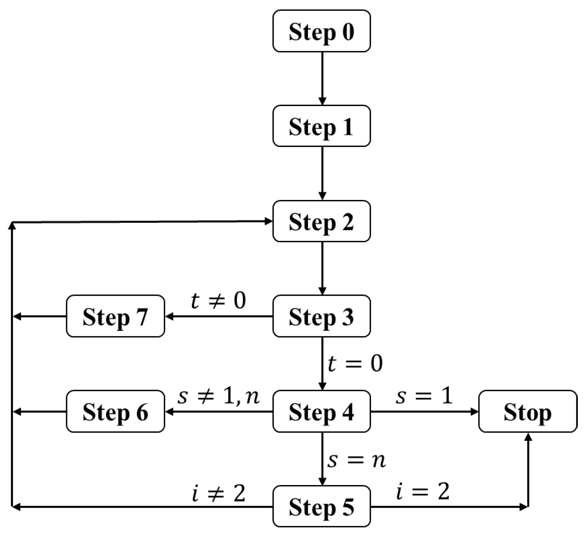
Figure 3.
A benchmark example of a communication infrastructure for a smart grid.
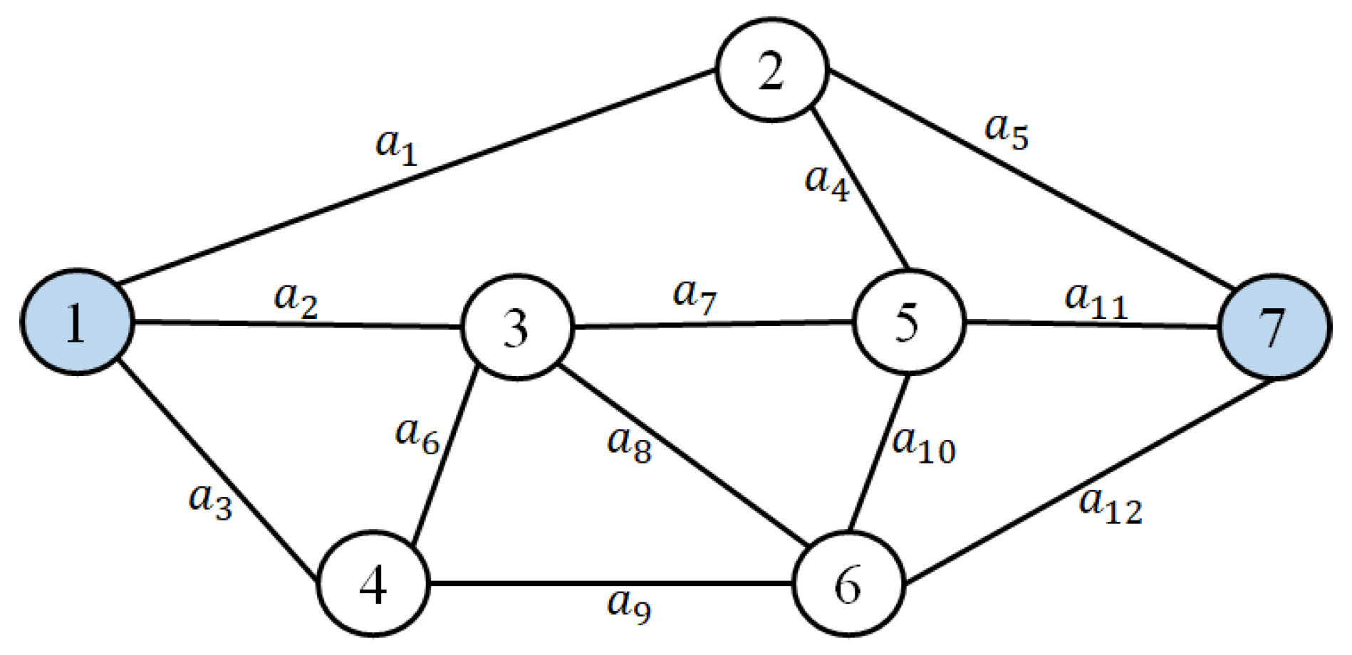
Figure 4.
The Arpanet topology taken from [51].
Figure 4.
The Arpanet topology taken from [51].
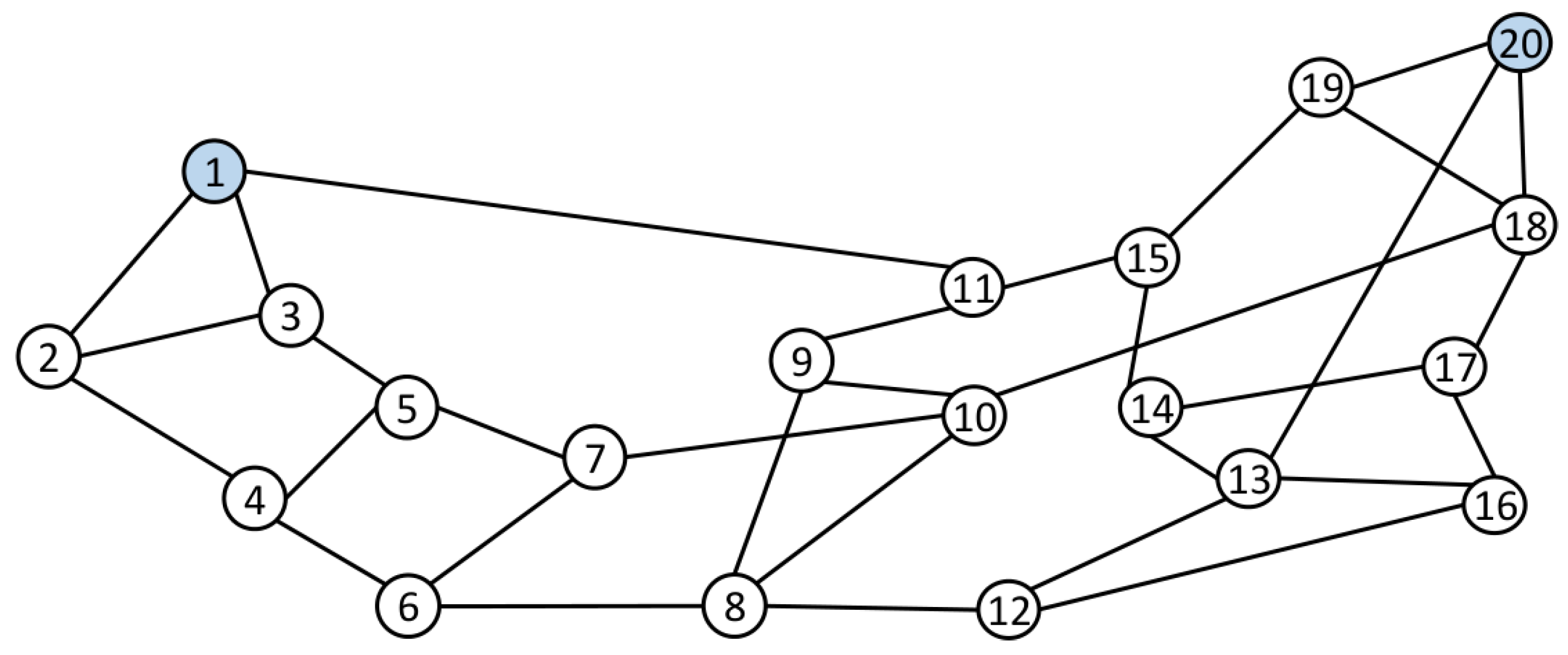
Figure 5.
The Dolan and Moré performance profiles for both algorithms based on CPU running times.
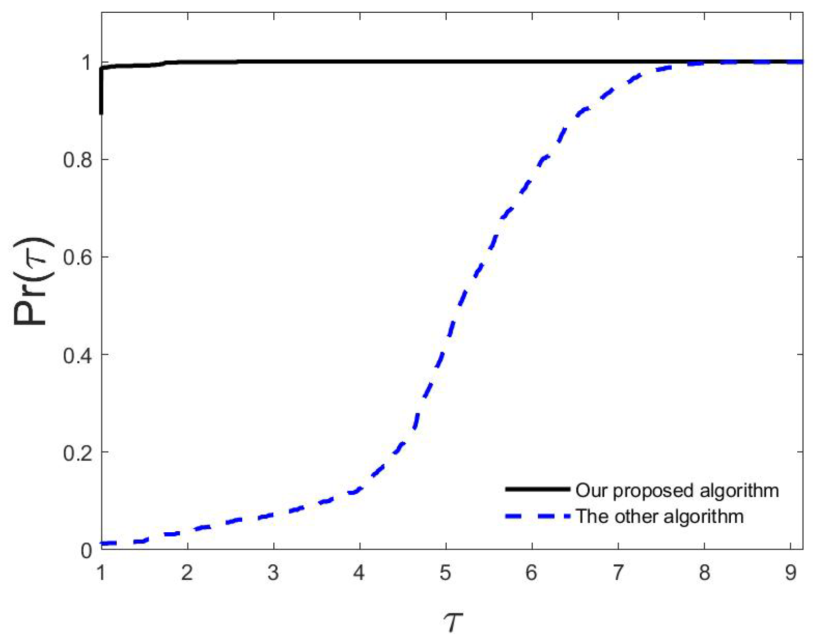
Table 3.
The final results on the Arpanet benchmark, depicted in Figure 4, with 1,610 MPs.
Table 3.
The final results on the Arpanet benchmark, depicted in Figure 4, with 1,610 MPs.
| d | ||||
|---|---|---|---|---|
| 96 | 283 | 0.0015 | 0.0054 | 3.5430 |
| 102 | 270 | 0.0012 | 0.0052 | 4.4396 |
| 108 | 254 | 0.0012 | 0.0051 | 4.3694 |
| 114 | 224 | 0.0011 | 0.0053 | 4.9603 |
| 120 | 204 | 0.0010 | 0.0050 | 5.1865 |
| 126 | 192 | 0.0009 | 0.0051 | 5.7419 |
| 132 | 177 | 0.0009 | 0.0050 | 5.6753 |
| 138 | 167 | 0.0009 | 0.0050 | 5.6062 |
| 144 | 147 | 0.0008 | 0.0072 | 8.5036 |
| 150 | 137 | 0.0011 | 0.0050 | 4.4366 |
| Geo. Mean | 0.0011 | 0.0053 | 5.2463 | |
Table 4.
The average data on the ten sets of randomly generated test problems.
| n | |||||
|---|---|---|---|---|---|
| 31 | 30369 | 12356 | 1.314 | 8.577 | 6.528 |
| 32 | 25518 | 10487 | 0.911 | 5.285 | 5.802 |
| 33 | 35999 | 14713 | 1.756 | 10.996 | 6.263 |
| 34 | 22646 | 9425 | 0.795 | 4.476 | 5.631 |
| 35 | 45378 | 18715 | 2.953 | 18.958 | 6.420 |
| 36 | 33208 | 13773 | 1.710 | 10.398 | 6.080 |
| 37 | 63354 | 26457 | 6.498 | 43.972 | 6.767 |
| 38 | 39762 | 16763 | 2.428 | 14.160 | 5.832 |
| 39 | 80121 | 33274 | 8.966 | 60.483 | 6.746 |
| 40 | 49725 | 20963 | 4.249 | 26.568 | 6.252 |
Disclaimer/Publisher’s Note: The statements, opinions and data contained in all publications are solely those of the individual author(s) and contributor(s) and not of MDPI and/or the editor(s). MDPI and/or the editor(s) disclaim responsibility for any injury to people or property resulting from any ideas, methods, instructions or products referred to in the content. |
© 2023 by the authors. Licensee MDPI, Basel, Switzerland. This article is an open access article distributed under the terms and conditions of the Creative Commons Attribution (CC BY) license (http://creativecommons.org/licenses/by/4.0/).
Copyright: This open access article is published under a Creative Commons CC BY 4.0 license, which permit the free download, distribution, and reuse, provided that the author and preprint are cited in any reuse.


