
Submitted:
08 November 2023
Posted:
08 November 2023
You are already at the latest version
Preprints on COVID-19 and SARS-CoV-2
Abstract
A simple bounded stochastic motion is employed for modelling equity price dynamics under shocks, where the prices are constrained to lie between two positive bounds. While the stochastic process has an inaccessible boundary, the other boundary is quasi-bounded, implying that the boundary can be breached if the probability leakage condition is met. The quasi-boundedness of the process at the boundary can thus provide an indicator of possible risk of equities under price shocks. Empirical calibration of model parameters of the proposed process for equities can be performed easily due to the availability of an analytically tractable probability density function which generates fat-tailed distributions consistent with empirical observations. The volatility and mean-reversion of the S&P500 dynamics calibrated by the process is positively and negatively co-integrated respectively with the VIX index representing the level of market distress. The process captures the high likelihood of Hertz’s default about two months earlier, using only information until that point, and before the firm filed for Chapter 11 bankruptcy in May 2020 as a result of the Covid-19 pandemic. Empirical calibration of the process for GameStop’s stock price shows that the short squeeze of the stock occurred when the condition for breaching an upper boundary was met on 14 January 2021, i.e., about two weeks before major short sellers closed out their positions with significant losses. The trading volume of the stock was positively co-integrated with the probability leakage ratio.
Keywords:
financial risk
; market distress
; predatory trading
; short squeeze
; constrained stochastic motion
; quasi-bounded process
; Covid-19
1. Introduction
Black (1986) argues that an efficient market is one in which price is within a factor 2 of value, i.e., the price is more than half of value and less than twice value in response to uninformed supply and demand flows. He further argues that the factor of 2 is arbitrary, but reasonable, in light of sources of uncertainty about value and the strength of the forces tending to cause prices to return to value. Therefore, prices are within an uncertainty band in which their dynamics are not random, but exhibit trends (see de Bondt and Thaler, 1985; DeLong et al.,1990; Hirshleifer and Subrahmanyam, 1998; Hong and Stein, 1999; Bouchaud et al, 2019). When prices move towards the limits of the band, some mean-reversion forces drive prices back to more reasonable levels. Studies including Fama and French (1988), Poterba and Summers (1988), Day and Huang (1990), Lux and Marchesi (2000), and Bouchaud et al. (2018) find empirical evidence that in the dynamics of various asset classes, such as stock indexes, commodities, bonds and currencies, mean-reversion represents a self-correcting mechanism and comes as a mitigating force against trend. For the purposes of pricing derivatives and simulations of future price movements, each stochastic process has to be properly modelled to resemble the empirical statistical properties of a given asset class. In view of studies of the existence of uncertainty bands, price trends and mean-reverting forces, a bounded stochastic process is needed to model the constrained stochastic motion of financial asset prices. For limited liability assets, such as coupon bonds and derivative securities with a finite number of bounded payouts, the use of a lognormal process does not address the upper bound constraint imposed by limited liability. Central banks of many countries also try to maintain their exchange rates within a particular range relative to the US dollar, e.g. the Hong Kong dollar. In addition, time series data of some financial observables, such as interest rates and variance rates, are typically confined to a band.
In this paper we propose a relatively simple stochastic model for financial observables which are constrained to lie between two positive bounds representing an uncertainty band. Generally, these two bounds are time varying. Driven by forecasting with time series decomposition, this model is not only capable of capturing most stylised facts of those financial observables, but is also highly intuitive. Specifically, we detrend the time series of the financial observables and simply concentrate on modelling just their fluctuations. While the proposed stochastic process has an inaccessible upper boundary, the lower boundary is quasi-bounded, implying that the lower boundary can be breached if the probability leakage condition is met as shown in Pesz (2002), Lo (2003), Silva et al. (2006), and Cardeal et al. (2007). Such a property is similar to the bounded exchange rate dynamics studied by Ingersoll (1997) and Larsen and Sørensen (2007), in which the exchange rate is completely bounded under all circumstances.
Given that the well-known Cox-Ingersoll-Ross (CIR) (1985) process allows the underlying variable to be quasi-bounded at the zero bound and is a mean-reverting process, we select CIR to represent the quasi-bounded process. The CIR model is popular among practitioners and is used for pricing various asset classes, such as equities, fixed income, commodities, foreign exchanges and their derivatives as in Carr (2020), and modelling variance of asset prices in Heston (1993). Because the CIR process has an analytically tractable probability density function, the calibration of model parameters for different financial observables can be performed easily. In terms of the calibrated model parameters, assessing the likelihood of future movements of these observables becomes feasible. In particular, we can determine whether or not the stochastic process is still bounded. As a result, the quasi-boundedness of the process at the lower boundary can provide an indicator of a possible downside risk of the corresponding observables, including equites in distress. We examine whether the dynamics of the S&P500 index (S&P) subject to market distress risk can be characterised by the quasi-bounded process. In addition, given that Hertz filed for Chapter 11 due to the impact of the Covid-19 pandemic on the car-rental industry, we investigate the relationship between the intensity of the pandemic’s spread, which triggered the firm’s financial distress, and its equity price dynamics derived from the model. The corresponding model parameters are related to the level of market distress in terms of the VIX index and the number of Covid-19 cases respectively, showing the validity of the model.
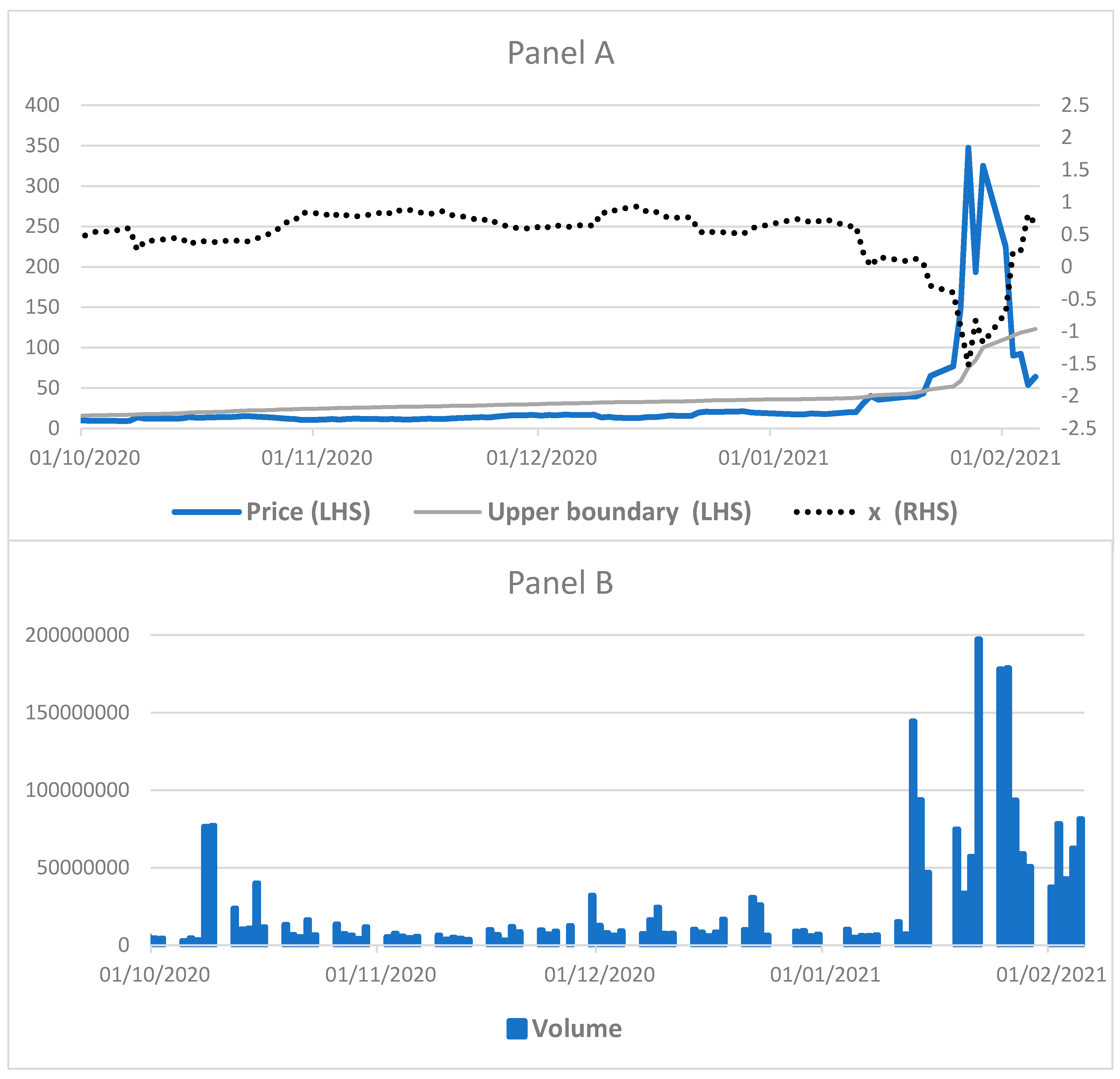
Retail trading activity in the US stock market has surged since late 2019, when some brokerages cut commissions to almost zero. Its impact on the market is demonstrated by the price action of GameStop (GME) as a result of co-ordinated buying through forums in January 2021, which put the low profile GME on the front pages of financial news organisations. Interest in GME emerged from individual investors on social media sites after they discovered the extreme short interest in the stock (139% of free float at the peak). These investors acted as a group to build buying pressure on a short squeeze, leading GME stocks to rise 57% to $31.4 on 13 January 2021, followed by another 27% jump the next day. On 27 January, the share price surged to $347 (see Figure 5) with the median target price among analysts of only $12.50. On the same day, some of the most prolific hedge funds lost the majority of their GME short positions at a substantial loss (See https://www.wsj.com/articles/melvin-capital-lost-53-in-january-hurt-by-gamestop-and-other-bets-11612103117 and the timeline at https://www.reuters.com/article/us-gamestop-hot-timeline-idUSKBN29W237).
Traders have a limited capacity, meaning that they cannot sustain losses beyond a certain point as illustrated by Brunnermeier and Pedersen (2005), particularly for funds which have redemption obligations for investors. In addition, their trading limits measured by value-at-risk act as constraints on keeping their positions. When stock prices shorted (longed) by traders surge (fall) beyond certain thresholds, the positions must be closed out due to those constraints. Brunnermeier and Oehmke (2014) argue that financial institutions may be vulnerable to predatory short selling. When the stock of a financial institution is shorted aggressively, leverage constraints imposed by short-term creditors can force the institution to liquidate long-term investments at fire sale prices. Brunnermeier et al. (2009) show that the illiquidity in the market suggests more scope for predators to make a profit as those traders need more time to close out their positions with larger movements in the prices. Stein (2009) demonstrates that another destabilising impact is crowding. Boehmer et al. (2008) and Diether et al. (2009) point out that high short-sale volume of a stock will attract positive-feedback on short selling trading. The mean reversion in the CIR process represents the market actions between long buyers and short sellers, which form an error-correction process in the price dynamics. The process allows the equity price to be quasi-bounded at an upper bound, which is the threshold imposed by constraints such as stop-loss limits forcing traders to close out short positions squeezed by co-ordinated buying. Their scramble to buy adds to the upward pressure on the stock's price. A surge in the equity price breaching the bound triggered by the short squeeze is conditional on the probability leakage ratio of the CIR process.
Lo et al. (2015) and Hui (2016) find that the quasi-bounded CIR process can describe the exchange rate dynamics and interest rate differentials of the Hong Kong dollar against the US dollar in a target zone, and the Swiss franc against the euro during the target zone regime of September 2011 to January 2015, respectively. Hui et al. (2022a) apply the quasi-bounded target-zone model to model yield curve control for Japanese government bonds. Using moving boundaries, the quasi-bounded process captures the price dynamics of Bitcoin and crude oil subject to crash risk under demand or supply shocks (see Hui et al., 2020a; Hui et al., 2020b); exchange rate dynamics under the floating-rate regime with crash risk and interventions (see Hui et al., 2022b; Hui et al., 2022c); and unemployment rate dynamics (see Hui et al., 2022d).
The paper is organised as follows. We present the model of the quasi-bounded process in the following Section. The calibrations of the equity price dynamics under market distress and short squeezes respectively are presented in Section 3. The relationships between the equity dynamics and market conditions are studied empirically and discussed in Section 4. The final section is the conclusion.
2. Methods
2.1. Modelling Constrained Stochastic Motion
A financial observable S is constrained to lie within the interval for . Both and are time-varying. It is well known that the moving average gives the trend component of the time series of S as shown in Ritschel et al. (2021) and Vinod et al. (2022). The time series of corresponds to the detrended series under the assumption of an additive decomposition of a time series. Based on qualifying the lower boundary of the financial observable in distress, historical data of the financial observable can be used as a guide to set a trading band from which the financial observable is not expected to escape. The historical trend of the financial observable can be measured by of its current and past values. For a financial observable in distress, the moving average can be scaled by a non-negative parameter such that forms a lower boundary for the movement of the financial observable. The parameter indicates how much market participants expect the maximum or extreme downside of holding the financial observable to be in terms of a fraction of the moving average of value . A smaller suggests the market expects wider fluctuations over short horizons. If no authority has been forced to offer “one-way bets" to short-lived speculative spurts, the financial observable can fluctuate with a relatively large margin within a band. Such specification of a lower boundary assumes market participants care about the behaviour of the financial observable over a time interval, rather than just its current value. The particular way in which past values of the financial observable are brought into play does not affect the qualitative results of our analysis.
Without assuming any distribution of the financial observable, the lower boundary SL is taken to be the number ( of standard deviations () from its mean : . If a normal distribution is assumed, the cumulative normal probabilities when the financial observable falls below the boundaries are 0.0668 and 0.0227, if is set equal to 1.5 and 2 respectively. It is noted that even when the financial observable is not normally distributed, 1.5 and 2-standard deviations still cover a large area under the distribution of the financial observable in a given time horizon, suggesting that falling to the lower boundary is in distress. The idea is similar to the analysis of currency crashes by Jurek (2014), who sets a threshold of a crash according to the strikes of the 25% delta and 10% delta options corresponding to 0.7 and 1.4 standard deviations, respectively, away from the exchange rates. The measure is also similar to value-at-risk (VaR), which is a statistical measure of the riskiness of financial entities or portfolios of assets. VaR is defined as the maximum expected loss at a pre-defined confidence level (say 95%) over a given time horizon. Intuitively, an asset with a sharp fall in its price at the 95th percentile (i.e. a 5% probability of such extreme loss during the sample period) suggests the asset price is under stress. The choice of the level of the boundary (provided that it is adequately low) does not affect the process of the financial observable dynamics. It is not necessary for the financial observable to breach the lower boundary to capture its dynamics.
The upper boundary can be defined similarly as for a parameter . The logarithm normalised fractional deviation x of S from is given by
where , and x = 0, when . Both and are adjustable parameters for the upper and lower boundaries of a band, respectively. It is not necessary for the two time-varying boundaries to be symmetric about the moving average . Accordingly, it is clear that the financial observable is confined to a drifting band with time-varying width. Similarly, regarding an upside shock, we can put the origin at an upper boundary by defining
The stochastic process of a financial asset is commonly modelled by the CIR process (see for example Heston, 1993). The CIR process allows the underlying variable to be quasi-bounded at the zero bound and is a mean-reverting process. Following this approach, we propose that the normalised financial observable x in Eq.(1) [ in Eq.(2)] follows the CIR process:
where dZ is a Wiener process with E[dZ] = 0 and E[dZ2] = dt. Here in the second stochastic term depends on the level of x, determines the speed of the mean-reverting drift towards the long-term mean . Following Feller’s classification of boundary points, it can be inferred there is a non-attractive natural boundary at infinity (i.e., inaccessible) and the one at the origin is a boundary of no probability leakage for : , and it is not otherwise (see Karlin and Taylor, 1981). In other words, it is a quasi-bounded process. The no-leakage condition ensures the financial observable will not breach the lower bound (the origin of x = 0); otherwise, it may pass through the lower bound. While the variance declines towards the boundary at x = 0, x could breach the boundary under the particular condition: >1.
The normalised financial observable x which is a fractional deviation of S from follows the CIR process by using the normalisation of Eq.(1) or (2). The implication is that the random fluctuation of the physical financial observable S is described by this stochastic process. The normalised financial observable dynamics thus contain information of the physical volatility of S. This suggests that a restoring force in the normalised financial observable dynamics will pull the random variable x away from the lower (upper) bound towards the long-term mean. Leakage through the bound occurs only when the fluctuations accompanied with a shock in the financial observable (in rare situations) shoot up drastically or the restoring force diminishes sharply. This is consistent with the observations in Bates (2012) in which volatility goes up or mean reversion, representing an error-correction process, drops during bad economic periods.
2.2. Probability Density Function
The probability density function (PDF) of x under the CIR process is given by:
where , , and , and is the modified Bessel function of the first kind of order . The associated asymptotic PDF will eventually approach the steady-state distribution, which is:
where is the gamma function. Given the PDF in Eq.(4), the parameters of the CIR process are calibrated by using market data in section 3.
Based on the calibration of the model parameters using the S&P in section 3, with the lower boundary and upper boundary Figure 1 shows the steady-state distributions in S based on Eq.(5) with three values of the long-term mean f 0.3, 1.0 and 1.5: the smaller is closer to the lower boundary, corresponding to S = 2268, 2797 and 3003 respectively. We use the model parameters for (Panel A), and 0.15 (Panel B), and = 0.05. The distributions with = 1.0 and 1.5 have their peaks at the right, showing the PDF decays at a slower rate than a Gaussian distribution at the left, suggesting the fat-tails effect with the probability of outlier negative returns. On the other hand, the distributions with = 0.3 have their peaks at the left and the probability of outlier positive returns. The different skewness of the distributions is consistent with the empirical observations of equity returns and both left- and right-skewed distributions for equities, depending on the sample periods of their studies.
Both panels show fatter left tails of the distributions with the mean further away from the lower boundary, demonstrating that the probability of outlier negative returns becomes more significant for the financial observable expected to increase in the near term. Comparison between Panels A and B where x increases from 0.05 to 0.15, the distributions have fatter tails and become hump shaped. Their skewness is sensitive to an increase in the volatility. The higher volatility increases the likelihood of a distress, which is reflected by the fatter left tails. The changes in the distributions with different model parameters demonstrate that the probability leakage condition of the quasi-bounded process is consistent with the left-skewed distributions for equities in distress.
3. Results
3.1. Calibrations of S&P500 Index in Distress
We examine whether the dynamics of the S&P in distress can be characterised by the quasi-bounded process. By using the log-likelihood function based on the PDF of Eq.(4) and the logarithm normalised x in Eq.(1), we can calibrate the model parameters of the process specified in Eq.(3). For the sample period, the calibration is conducted by applying the maximum likelihood estimation (MLE) to the daily spot index of the S&P data from 1 January 1990 to 20 June 2020. Figure 2 (Panel A) shows the S&P in S and the associated moving lower and upper boundaries with the parameters of and on the 50-day moving average, and the normalised index in x of the time series. Market data used in this paper are from Bloomberg.
Based on the 1-year rolling window estimations results, Figure 3 reports statistically significant estimates of the drift term (Panel A) with the respective z-statistic maintaining above the value of 1.96 (i.e., at the 5% significance level) when is above 0.02. was in the range from 0.02 to 0.12 for most of the time and dropped sharply under shocks or crashes in the market. As the S&P dropped towards its lower boundary during these crashes, the mean-reverting force weakened with the dropped . It is noted that the estimation of became insignificant (not significantly different from zero) in very short periods of time after the crashes. Subsequently, the estimation rebounded to the 0.04 level with the z-statistic higher than 1.96. Panel B shows a steady estimated mean with the values ranging between 0.7 and 1.2 with the corresponding z-statistic staying above the 1.96 level. Similar to the changes in , the estimation of became insignificant in very short periods of time after the crashes. The mean-reverting force, which is represented by the parameters and is estimated to be present during the estimation period.
The volatility σx, which is displayed in Panel C, is estimated to be between 0.02 and 0.14. The corresponding z-statistic is much higher than 1.96, indicating that the estimated σx is highly significant. The results suggest that the estimation of the square-root-process part of the quasi-bounded dynamics is robust. The volatility increased sharply during 2008-2009 when the global financial crisis emerged, and the Covid-19 outbreak in March 2020.
As the probability leakage condition of can portray the crash risk of the S&P at the lower boundary, Panel D displays this measure to identify periods with the leakage condition greater than 1. The measure was generally below 0.01, suggesting that the crash risk was immaterial when the S&P was bounded above the lower boundary. In recent history, the measure rose sharply and breached 1.0 on 23 July 2002 (the dotcom bubble crash), 9 October 2008 (the subprime mortgage crisis), 8 August 2009 (the global financial crisis) and 9 March 2020 (the Covid-19 pandemic), with the existence of the leakage condition when the S&P fell sharply. The diminishing mean-reverting force in the S&P dynamics and the existence of the leakage condition reflect that the crash risk built up at the lower boundary during the crashes.
We use the Breusch-Godfrey serial correlation Lagrange-multiplier test to study autocorrelation in the errors of the model estimations. The test makes use of the residuals from the model and a test statistic is derived from these. The null hypothesis is that there is no serial correlation of any order up to p. Panel E shows that despite some rejections of null hypothesis (i.e., low p-values), majority of the tests accept the hypothesis that the residuals are not serially correlated up to 5 days, indicating that the estimations are adequate.
3.2. Calibrations of Hertz Equity Price in Distress
To investigate how financial distress affects equity price dynamics, we calibrate the dynamics of the Hertz equity (HTZ) price according to the quasi-bounded process. Hertz filed voluntary petitions for re-organisation under Chapter 11 on 22 May 2020 as the Covid-19 pandemic crushed the car-rental industry. The sample period covers the daily price of HTZ from 18 August 2014 to 31 August 2020. Panel B of Figure 2 shows the price of HTZ in S and the associated moving lower and upper boundaries with the parameters of and on the 50-day moving average, and the normalised price in x. The lower and upper boundaries correspond to about 2.4 standard deviations respectively.
Based on the 2-year rolling window estimations, Figure 4 reports statistically significant estimates of the drift term (Panel A) with the corresponding z-statistic staying above the value of 1.96 (i.e., at the 5% significance level) when is above 0.02. was between 0.02 and 0.1 during most of the time. It dropped sharply and was not significantly different from zero on 16 March 2020. As the HTZ price dropped towards its lower boundary during March 2020, the mean-reverting force in its dynamics weakened substantially. Panel B shows a steady estimated mean with the values ranging between 0.5 and 0.8, and the corresponding z-statistic staying above the 1.96 level. Similar to the changes in , the estimation of became insignificant on 16 March 2020. The volatility , which is displayed in Panel C, is estimated to take the value between 0.06 and 0.13. The corresponding z-statistic is much higher than 1.96, indicating that the estimated is highly significant.
Panel D shows the measure of the probability leakage condition which was below 0.2 before March 2020, suggesting that the default risk was not significant as the HTZ price was bounded above the lower boundary. The measure rose sharply and breached 1.0 on 16 March 2020 with the existence of the leakage condition when the HTZ price fell sharply. While the HTZ price was bounded above the lower boundary for much of the time, as indicated by its dynamics, the condition for breaching the boundary was met on 16 March 2020 using only information until that point, about two months before the company filed for bankruptcy. The existence of the leakage condition suggests the default risk of the firm occurs and its default probability accumulates.
In summary, we find empirical evidence that the quasi-bounded process adequately describes the dynamics of both the S&P and HTZ price by incorporating a feature of a lower boundary representing the level for a crash or financial distress. By using the MLE estimation, the estimated parameters are found to be time-varying. The mean-reverting force, which is represented by the parameters and , are estimated to be present during the estimation period. The diminishing mean-reverting force in the HTZ price dynamics and the existence of the leakage condition reflect the firm’s default risk built up (i.e., an increase in default probability) in March 2020 under financial distress.
3.3. Calibration of GameStop Stock Price Dynamics under Short Squeezes
The calibration is conducted by applying the MLE and the logarithm normalised in Eq.(2) to the daily GME price data from 1 January 2017 to 21 January 2021. Figure 5 (Panel A) shows the GME price in S and the associated moving upper boundary with the parameters of on the 50-day moving average, and the transformed equity price in x. The upper boundary corresponds to about 2.5 standard deviations covering the probability of 99.38%.
Figure 5.
GameStop stock price in S-scale and x-scale, upper boundary [in S on 50-day moving average (Panel A) and trading volume (Panel B).
Figure 5.
GameStop stock price in S-scale and x-scale, upper boundary [in S on 50-day moving average (Panel A) and trading volume (Panel B).
Using the 2-year rolling window, Figure 6 reports statistically significant estimates of the drift term (Panel A) with the z-statistic above the value of 1.96 (i.e., at the 5% significance level). When the GME price surged sharply in January 2021, fell and was not significantly different from zero on 14 January 2021. Panel B shows the estimated mean which is significant with the corresponding z-statistic above the 1.96 level until the price spiked in January 2021. The results show that the mean-reverting force, which is represented by and was present in the GME price dynamics during the estimation period and diminished under the short squeeze in January 2021. The volatility σx, which is displayed in Panel C, is estimated to have an increasing trend, and jumped in January 2021. The corresponding z-statistic is much higher than 1.96, indicating that the estimation of the square-root-process part of the quasi-bounded dynamics is robust.
As the probability leakage condition of portrays the likelihood of the GME price breaching the upper boundary under the short squeeze, Panel D displays this measure to identify periods with the leakage condition greater than 1. The measure was in general below 0.05, suggesting that the short squeeze was not relevant to the GME price bounded below the upper boundary. The measure rose sharply and breached 1.0 on 14 January 2021 with the existence of the leakage condition when the GME price escalated. The diminishing mean-reverting force in the GME price dynamics and the existence of the leakage condition indicate the short squeeze built up through co-ordinated buying.
4. Discussion
4.1. The Dynamic Relationship of S&P500 Index Dynamics with Market Stress Condition
To test the validity of incorporating crash/distress risk into the model, a co-integration analysis is used to test the relationship between the dynamics of the S&P and the VIX. The VIX, which is the US stock-market volatility index derived from the price inputs of the S&P500 Index options, gauges the level of risk aversion anticipated by market participants to put capital into the market. It captures the information of market stress conditions embedded in option prices. This is noted as the model parameters based on the MLE are estimated using the S&P data only, without any information from the option market.
If a long-run equilibrium relationship exists between the model parameters and VIX, their short-run dynamics can be studied through the following dynamical error-correction representation:
where is either , or at time t, and is less than zero. is logarithm of the VIX at time t-1. Under this representation, the logarithm of model parameters () and the mean level (represented by ) will respond to stochastic shocks (represented by ) and also the long-run equilibrium deviation in the previous period (i.e., ). The mean level in the original price measure of S is used instead of , because risk sentiment in the market is based on the level of the price in S not in x normalised by the time-varying upper and lower boundaries. The estimated speed of adjustment (i.e., ) should be negative and nonzero for the co-integration relationship to be validly specified by the error-correction. In terms of absolute magnitude, a larger estimated value of reflects a higher sensitivity of to the long-run equilibrium deviation in the previous period.
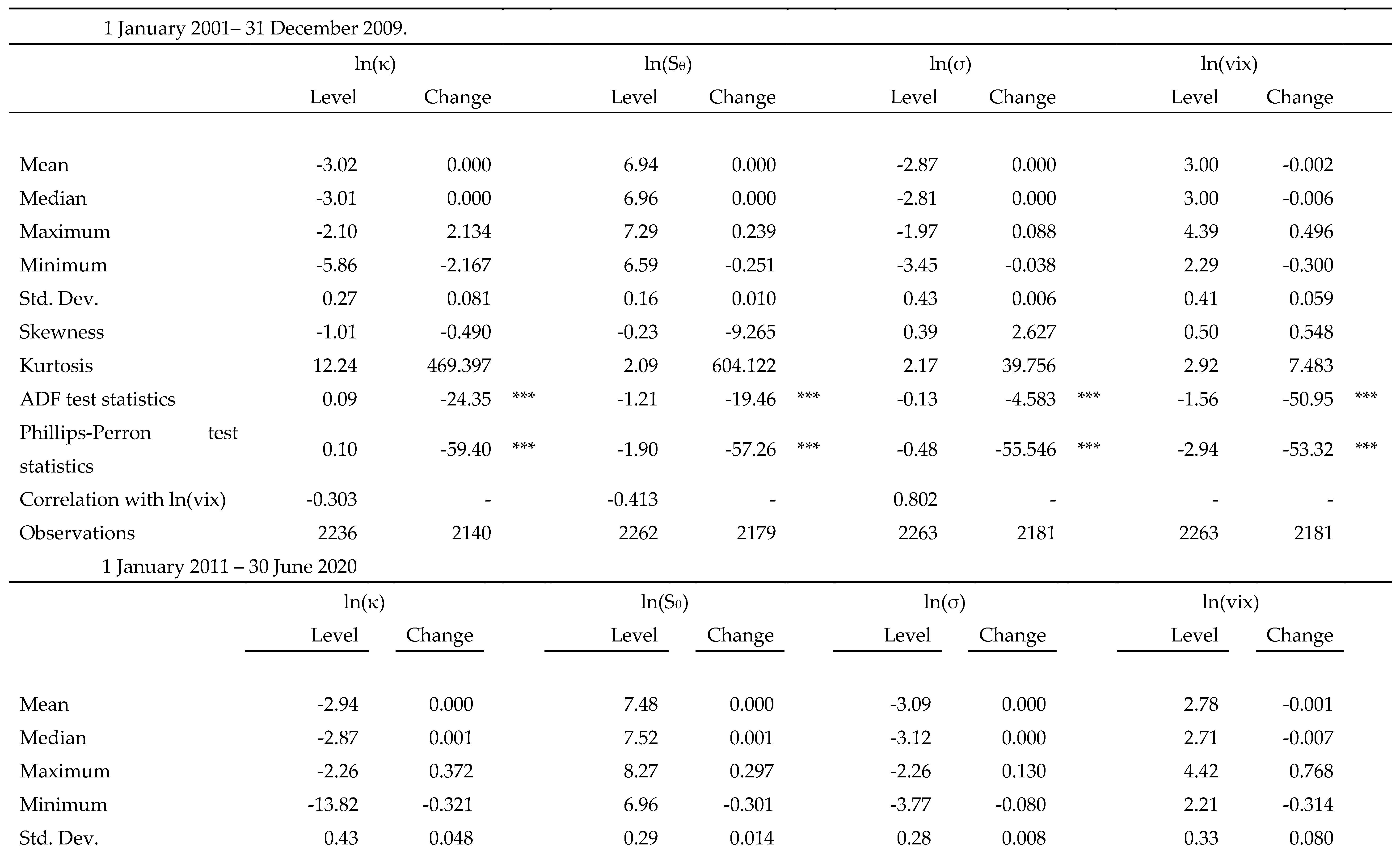
As there was a structural break during the global financial crisis in 2009, the estimation is conducted at a daily frequency for the pre-crisis period from 1 January 2001 to 31 December 2009, and the post-crisis period from 1 January 2011 to 30 June 2020. Table 1 reports the summary statistics, correlation coefficient and the respective Augmented Dickey–Fuller (ADF) test results for the variables both in levels and first differences for the pre- and post-crisis periods respectively. The ADF test results reflect that the existence of a unit root for ln, ln(, ln and logarithm value of the VIX [ln in level form cannot be rejected at the 10% significance level. Nonetheless, the respective ADF tests for the first differenced variables indicate no presence of unit root at the 1% level. Thus, the above results suggest that these variables are all co-integrated with the same order I (i.e., I(1)).
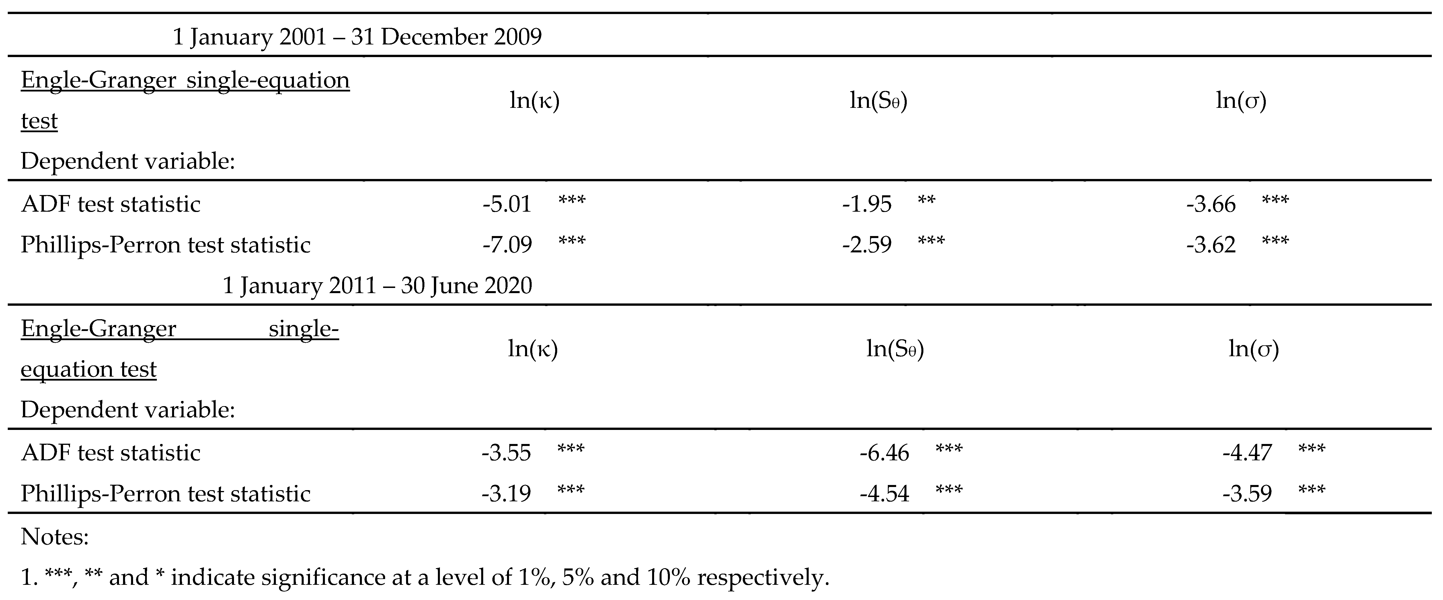
We adopt the Engle–Granger (1987) single-equation test to test the co-integration relationship between [ln, ln(, ln] and ln. This test essentially examines whether the residuals of the linear combinations between i. ln and ln; ii. ln( and ln; and iii. ln and ln are stationary. Table 2 reports the co-integration tests between ln(VIX) and [ln, ln(, ln with the ordinary least squared regression residuals being tested by both the ADF and Phillips-Perron tests for the pre- and post-crisis periods respectively. Overall, the results favour the alternative hypothesis of the presence of at least one co-integrating vector of ln and [ln, ln(, ln respectively, given the statistical significances at the 1% or 5% levels.
Table 3 shows that the co-integrating vectors expressed by β between ln and [ln, ln(, lnare estimated to be [-0.2, -0.14, 0.83] and [-0.52), -0.14 and 0.56] in the pre-crisis and post-crisis periods respectively at the 1% level. The estimated negative coefficients indicate that a higher VIX would decrease and , holding other things constant. Intuitively, the negative relationship suggests that when the VIX increases, the crash risk of the S&P rises, with the weakened mean-reversion force in the S&P dynamics. On the other hand, the estimated positive coefficient for shows that a higher VIX would increase as expected.
As reported in Table 4, the estimates of the speed of adjustment (that is, αy) for [ln, ln( and ln are negative with [-0.04, -0.005, -0.04] and [-0.01, -0.001, -0.0045] in the pre-crisis and post-crisis periods respectively, indicating that the model parameters will subsequently adjust to restore the long-run equilibrium. This demonstrates a valid error- correction specification and the presence of a self-restoring force, which will close the gaps of the link between the model parameters and VIX.
4.2. The Relationship between Hertz Equity Price Dynamics and Covid-19
Given that Hertz filed for Chapter 11 due to the impact of the Covid-19 pandemic on the car-rental industry, we investigate the relationship between the intensity of the pandemic’s spread, which triggered the firm’s financial distress, and its equity price dynamics derived from the model. We estimate the following simple linear regression:
where is the model parameters {, , }, is the number of new confirmed Covid-19 cases in the US, and a and b are the coefficients to be estimated.
As the first confirmed Covid-19 case in the US was on 22 January 2020 and the quasi-bounded process for HTZ was no longer bounded after 16 March 2020, the estimation is conducted for the period between these two dates. Figure 7, Figure 8 and Figure 9 show the scatter plots of the model parameters and the number of daily new Covid-19 cases in the US in logarithm. The data of Covid-19 cases are compiled by the Johns Hopkins University Center for Systems Science and Engineering (JHU CCSE) from various sources at https://data.humdata.org/dataset/novel-coronavirus-2019-ncov-cases. The coefficients , are estimated to be [-2.37,-0.16] for , [-0.32, -0.01] for and [-2.55, 0.019] for respectively. All the estimates of coefficients are statistically significant at the 1% level. The of 0.777, 0.463 and 0.737 for , and respectively are reasonably high.
The negative coefficients and show a negative relationship between the mean reversion (represented by and ) and the number of Covid-19 cases in the US. Conversely, the relationship in terms of between the volatility and the number of confirmed cases is positive. An increase in the number of confirmed cases weakened the mean-reverting force, but enhanced the volatility in the HTZ price dynamics, suggesting an increased default risk of the firm due to the Covid-19 pandemic in the US. The results are consistent with those of the model calibration results and the measure of the probability leakage condition at the lower boundary for the HTZ price in section 3.2.
4.3. The Relationship between the GameStop Stock Price Dynamics and Trading Volume
A co-integration analysis is used to test the relationship between the mean reversion in the GME price dynamics and the daily trading volume by Eq.(7), where is or at time t, and is the logarithm of the trading volume at time t-1. The estimation is conducted at a daily frequency starting from 1 January 2019 to 21 January 2021. Table 5 reports the summary statistics, correlation coefficient and the respective ADF test results for the variables both in levels and first differences. The ADF test results reflect that the existence of a unit root for , and the logarithm value of the trading volume in level form cannot be rejected at the 10% significance level. Nonetheless, the respective ADF tests for the first differenced variables indicate no presence of a unit root at the 1% level. Thus, the above results suggest that these three variables are all co-integrated of same order I (i.e., I(1)).
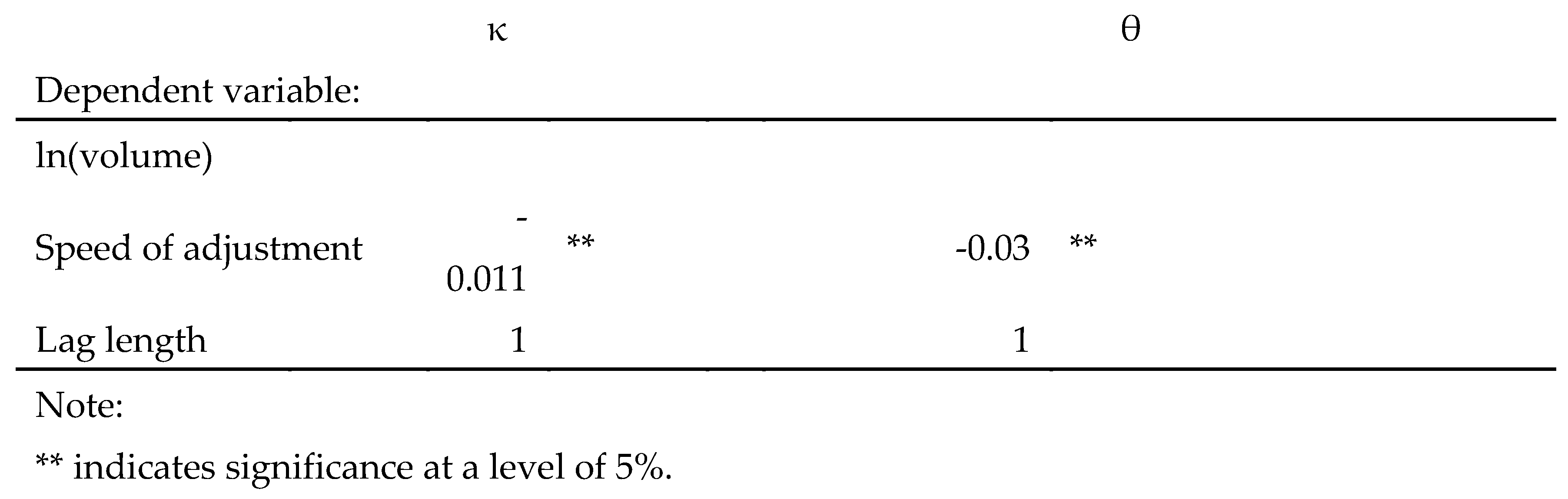
Table 6 reports the co-integration tests between ln and (, . The results favour the alternative hypothesis of the presence of at least one co-integrating vector between ln and , respectively, given the statistical significance for and at the 5% or 1% levels. Table 7 shows that the co-integrating vectors (expressed by β) between ln and (, are estimated to be -0.003, and -0.15 at the 1% level respectively. The estimated negative coefficients indicate that a higher trading volume reduces and , suggesting that the restoring force in the GME price dynamics weakens with a higher trading volume. In Table 8, the estimates of the speed of adjustment (αy) for and are negative, showing that the model parameters subsequently adjust to restore the long-run equilibrium. This demonstrates a valid error-correction specification, which will close the gap between the parameters and the trading volume.
5. Conclusion
In this paper a simple stochastic approach has been presented for modelling financial observables which are constrained to lie between two positive bounds. The model is not only capable of capturing most stylised facts of those financial observables but is also highly intuitive. While the proposed stochastic process has an inaccessible boundary, the other boundary is quasi-bounded, implying that the quasi-bounded boundary can be breached if the probability leakage condition is met. The quasi-boundedness of the process at the boundary can thus provide us with an indicator of possible risk of the corresponding observables. An empirical calibration of the model parameters of the proposed process for different financial observables can also be performed easily due to the availability of an analytically tractable probability density function. Hence, in terms of the calibrated model parameters, assessing the likelihood of future movements of these observables becomes feasible.
The empirical results show that the S&P500 dynamics can be calibrated according to the quasi-bounded process, in which the volatility and mean reversion are positively and negatively co-integrated respectively with the VIX index, representing the market distress risk implied in the option market. The process also captures the default risk incorporated in stock prices. Hertz filed for Chapter 11 bankruptcy in May 2020 as a result of the Covid-19 pandemic. The volatility and mean reversion of the calibrated Hertz stock price dynamics are positively and negatively related, respectively, to the number of Covid-19 cases. The process indicates a high likelihood of default in terms of the probability leakage condition at the lower boundary in March 2020 using only information until that point. We leave the investigation of a larger sample of companies in distress for future research.
The proposed stochastic approach is able to model equity price dynamics under a short squeeze. A quasi-bounded moving upper bound is the threshold imposed by constraints, such as stop-loss limits forcing traders to close out their short-selling positions squeezed by co-ordinated long buying. Calibration of the process for the GameStop stock price shows that the quasi-bounded property can adequately describe the price dynamics. The model captures the short squeeze of the stock as indicated by its price dynamics, when the probability leakage condition for breaching the upper bound was met on 14 January 2021 using only information until that point, i.e., about two weeks before major short sellers closed out their positions with a significant loss. The trading volume of the stock is negatively co-integrated with the mean-reversion of the dynamics, suggesting overshooting prices with increased trading volume during co-ordinated short squeezes.
Author Contributions
C.-H.H. and C.-F.L. are responsible for proposing the model and deriving the corresponding stochastic processes. C.-H.L. is responsible for performing the calibration of model parameters. All authors have read and agreed to the published version of the manuscript.
Funding
This research received no external funding.
Institutional Review Board Statement
Not applicable.
Informed Consent Statement
Not applicable.
Data Availability Statement
The datasets used in this paper are available from Bloomberg and the Johns Hopkins University Center for Systems Science and Engineering (JHU CCSE) at https://data.humdata.org/dataset/novel-coronavirus-2019-ncov-cases.
Acknowledgments
The views expressed in this paper are the authors’ and do not represent those of the Hong Kong Monetary Authority.
Conflicts of Interest
The authors declare no conflict of interest.
References
- Bates, D. U.S. stock market crash risk, 1926-2010. Journal of Financial Economics 2012, 105, 229–259. [Google Scholar] [CrossRef]
- Black, F. Noise. Journal of Finance 1986, 41, 529–543. [Google Scholar] [CrossRef]
- Boehmer, E.; Jones, C.M.; Zhang, X. Which shorts are informed? Journal of Finance 2008, 63, 491–527. [Google Scholar] [CrossRef]
- de Bondt, W.; Thaler, R.H. Does the stock market overreact? Journal of Finance 1985, 42, 557–581. [Google Scholar] [CrossRef]
- Bouchaud, J.P.; Ciliberti, S.; Lempérière, Y.; Majewski, A.; P Seager, P.; Sin Ronia, K. 2018. Black was right: Price is within a factor 2 of value. risk.net November, 1-4.
- Bouchaud, J.P.; Krueger, P.; Landier, A.; Thesmar, D. Sticky expectations and the profitability anomaly. Journal of Finance 2019, 74, 639–674. [Google Scholar] [CrossRef]
- Boyer, B.; Mitton, T.; Vorkink, K. Expected idiosyncratic skewness. Review of Financial Studies 2010, 23, 169–202. [Google Scholar] [CrossRef]
- Brunnermeier, M.K.; Pedersen, L.H. Predatory trading. Journal of Finance 2005, 60, 1825–1863. [Google Scholar] [CrossRef]
- Brunnermeier, M.K.; Nagel, S.; Pedersen, L.H. Carry trades and currency crashes. NBER Macroeconomics Annual 2009, 23, 313–347. [Google Scholar] [CrossRef]
- Brunnermeier, M.K.; Oehmke, M. Predatory short selling. Review of Finance 2014, 18, 2153–2195. [Google Scholar] [CrossRef]
- Cardeal, J.A.; de Montigny, M.; Khanna, F.C.; Rocha Filho, T.M.; Santana, A.E. Galilei-invariant gauge symmetries in Fokker-Planck dynamics with logarithmic diffusion and drift terms. Journal of Physics A: Mathematical and Theoretical 2007, 40, 13467. [Google Scholar] [CrossRef]
- Carr, P.; Itkin, A.; Muravey, D. Semi-closed form prices of barrier options in the time-dependent CEV and CIR models. Journal of Derivatives 2020, 28, 26-5. [Google Scholar] [CrossRef]
- Conrad, J.; Dittmar, R.F.; Ghysels, E. Ex ante skewness and expected stock returns. Journal of Finance 2013, 68, 85–124. [Google Scholar] [CrossRef]
- Cox, J.C.; Ingersoll, J.E.; Ross, S.A. A theory of the term structure of interest rates. Econometrica 1985, 53, 385–407. [Google Scholar] [CrossRef]
- Day, R.; Huang, W. Bulls, bears and market sheep. Journal of Economic Behavior and Organization 1990, 14, 299–329. [Google Scholar] [CrossRef]
- DeLong, J.; Bradford, A.; Shleifer, A.; Summers, L.H.; Waldmann, R.J. Positive feedback investment strategies and destabilizing rational speculation. Journal of Finance 1990, 45, 379–395. [Google Scholar] [CrossRef]
- Diether, K.B.; Lee, K.H.; Werner, I.M. Short sale strategies and return predictability. Review of Financial Studies 2009, 22, 575–607. [Google Scholar] [CrossRef]
- Engle, R.F.; Granger, C.W.J. Co-integration and error correction: Representation, estimation and testing. Econometrica 1987, 55, 251–276. [Google Scholar] [CrossRef]
- Fama, E.F.; French, K.R. Permanent and temporary components of stock prices. Journal of Political Economy 1988, 96, 246–273. [Google Scholar] [CrossRef]
- Heston, S.L. A closed-form solution for options with stochastic volatility with applications to bond and currency options. Review of Financial Studies 1993, 6, 327. [Google Scholar] [CrossRef]
- Hong, H.; Stein, J. A unified theory of underreaction, momentum trading, and overreaction in asset markets. Journal of Finance 1999, 54, 2143–2184. [Google Scholar] [CrossRef]
- Hui, C.H.; Lo, C.F.; Fong, T. Swiss franc's one-sided target zone during 2011-2015. International Review of Economics and Finance 2016, 44, 54–67. [Google Scholar] [CrossRef]
- Hui, C.H.; Lo, C.F.; Chau, P.H.; Wong, A. Does Bitcoin behave as a currency?: A standard monetary model approach. International Review of Financial Analysis 2020a, 70, 101518. [Google Scholar] [CrossRef]
- Hui, C.H.; Lo, C.F.; Cheung, C.H.; Wong, A. Crude oil price dynamics with crash risk under fundamental shocks. North American Journal of Economics and Finance 2020b, 54, 101238. [Google Scholar] [CrossRef]
- Hui, C.H.; Wong, A.; Lo, C.F. A note on modelling yield curve control: A target-zone approach. Finance Research Letters 2022a, 49, 103076. [Google Scholar] [CrossRef]
- Hui, C.H.; Lo, C.F.; Liu, C.H. Exchange rate dynamics with crash risk and interventions. International Review of Economics and Finance 2022b, 79, 18–37. [Google Scholar] [CrossRef]
- Hui, C.H.; Lo, C.F.; Liu, C.H. Modelling foreign exchange interventions under Rayleigh process: Applications to Swiss franc exchange rate dynamics. Entropy 2022c, 24, 888. [Google Scholar] [CrossRef] [PubMed]
- Hui, C.H.; Lo, C.F.; Ip, H.Y. Modelling asymmetric unemployment dynamics: The logarithmic-harmonic potential approach. Entropy 2022d, 24, 400. [Google Scholar] [CrossRef]
- Ingersoll, J.E., Jr. Valuing foreign exchange rate derivatives with a bounded exchange process. Review of Derivatives Research 1997, 1, 159–181. [Google Scholar] [CrossRef]
- Jurek, J.W. Crash-neutral currency carry trades. Journal of Financial Economics 2014, 113, 325–347. [Google Scholar] [CrossRef]
- Karlin, S.; Taylor, H.M. 1981. A Second Course in Stochastic Processes. Academic Press, New York.
- Kent, D.; Hirshleifer, D.; Subrahmanyam, A. Investor psychology and security market under- and over-reactions. Journal of Finance 1998, 53, 1839–1885. [Google Scholar]
- Larsen, K.S.; Sørensen, M. A diffusion model for exchange rates in a target zone. Mathematical Finance 2007, 17, 285–306. [Google Scholar] [CrossRef]
- Lo, C.F. Exact propagator of the Fokker–Planck equation with logarithmic factors in diffusion and drift terms. Physics Letters A 2003, 319, 110–113. [Google Scholar] [CrossRef]
- Lo, C.F.; Hui, C.H.; Fong, T.; Chu, S.W. A quasi-bounded target zone model – Theory and application to Hong Kong dollar. International Review of Economics and Finance 2015, 37, 1–17. [Google Scholar] [CrossRef]
- Lux, T.; Marchesi, M. Volatility clustering in financial markets: a microsimulation of interacting agents. International Journal of Theoretical and Applied Finance 2000, 3, 675–702. [Google Scholar] [CrossRef]
- MacKinnon, J.G. Numerical distribution functions for unit root and cointegration test. Journal of Applied Econometrics 1996, 11, 601–618. [Google Scholar] [CrossRef]
- Neuberger, A.; Payne, R. The skewness of the stock market over long horizons. Review of Financial Studies 2021, 34, 1572–1616. [Google Scholar] [CrossRef]
- Pesz, K. A class of Fokker-Planck equations with logarithmic factors in diffusion and drift terms. Journal of Physics A: Mathematical and General 2002, 35, 1827–1832. [Google Scholar] [CrossRef]
- Poterba, J.M.; Summers, L. Mean reversion in stock prices: Evidence and implications. Journal of Financial Economics 1988, 22, 27–59. [Google Scholar] [CrossRef]
- Ritschel, S.; Cherstvy, A.G.; Metzler, R. Universality of delay-time averages for financial time series: analytical results, computer simulations, and analysis of historical stock-market prices. Journal of Physics: Complex 2021, 2, 045003. [Google Scholar] [CrossRef]
- Silva, E.M.; Rocha Filho, T.M.; Santana, A.E. Lie symmetries of Fokker-Planck equations with logarithmic diffusion and drift terms. Journal of Physics: Conference Series 2006, 40, 150–155. [Google Scholar] [CrossRef]
- Stein, J. Sophisticated investors and market efficiency. Journal of Finance 2009, 64, 1517–1548. [Google Scholar] [CrossRef]
- Vinod, D.; Cherstvy, A.G.; Metzler, R.; Sokolov, I.M. Time-averaging and nonergodicity of reset geometric Brownian motion with drift. Physical Review E 2022, 106, 034137. [Google Scholar] [CrossRef] [PubMed]
Figure 1.
S&P500 Index distributions with different values of model parameters x, and under the normalisation on 1 November 2018.
Figure 1.
S&P500 Index distributions with different values of model parameters x, and under the normalisation on 1 November 2018.
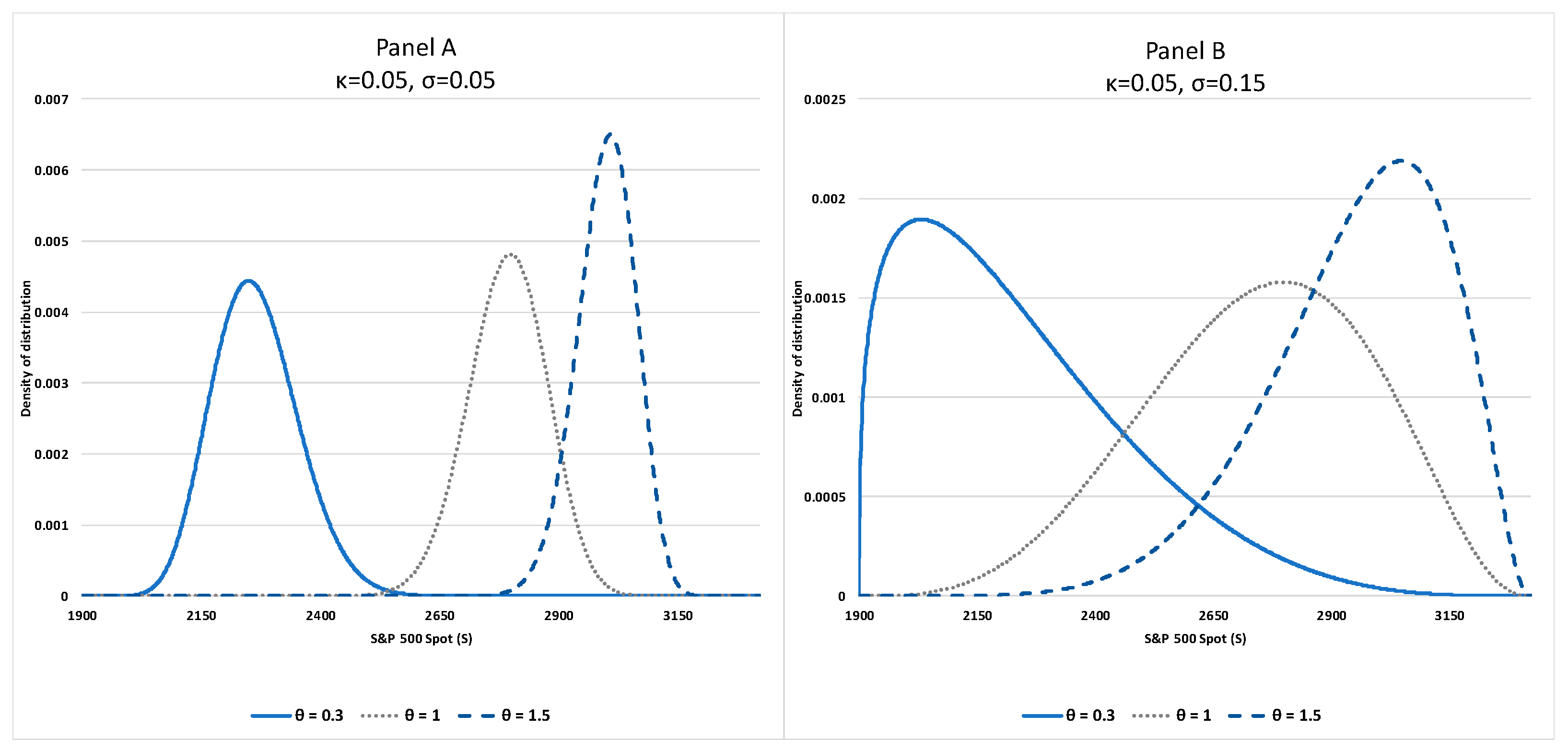
Figure 2.
S&P500 Index (Panel A) and Hertz stock price (Panel B) in S-scale and x-scale, and upper and lower boundaries in S with and for S&P500 Index and and for Hertz stock price on 50-day moving average.
Figure 2.
S&P500 Index (Panel A) and Hertz stock price (Panel B) in S-scale and x-scale, and upper and lower boundaries in S with and for S&P500 Index and and for Hertz stock price on 50-day moving average.
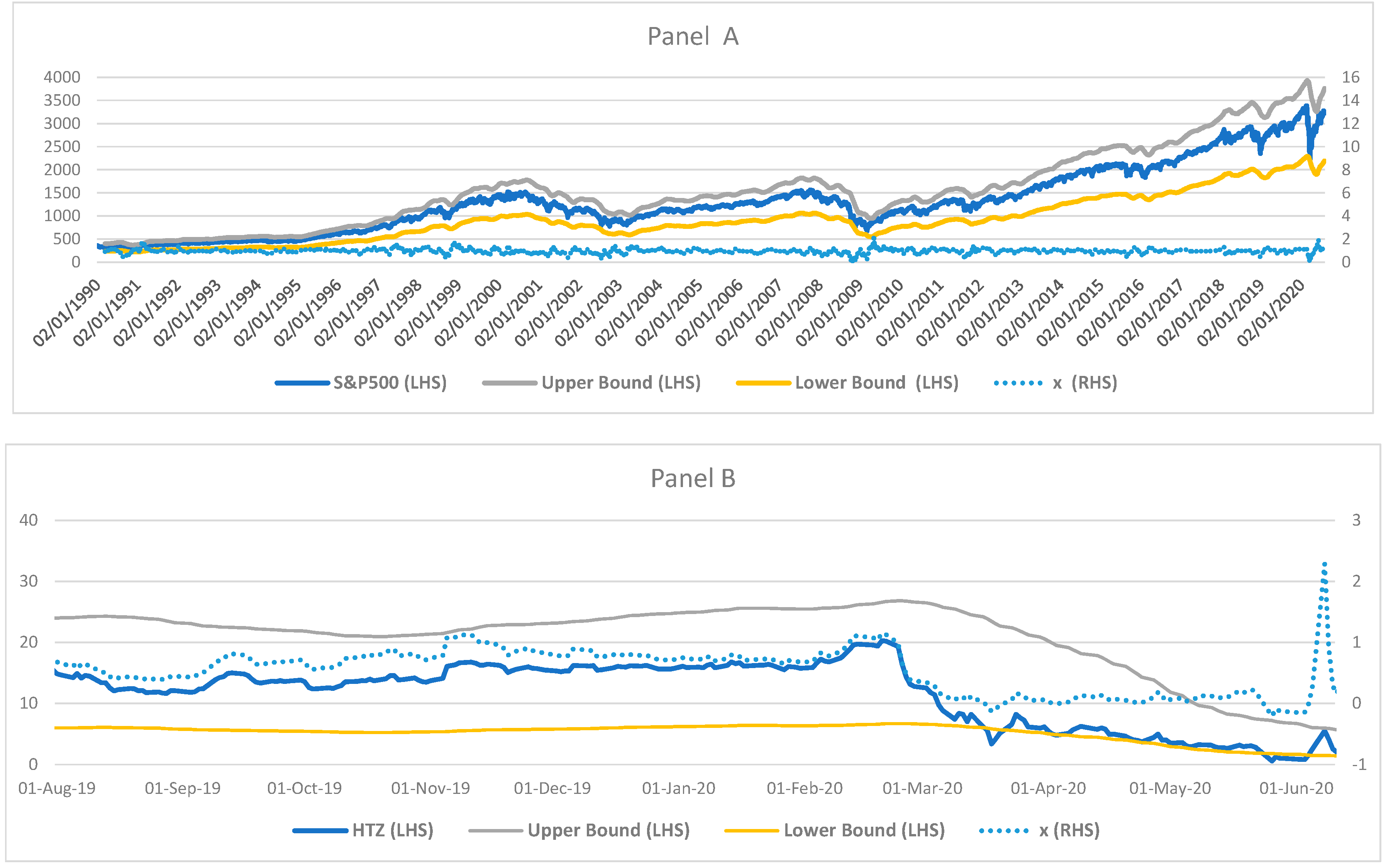
Figure 3.
Estimated Panel A), (Panel B), x Panel C), corresponding z-statistic, leakage ratio () (Panel D) of S&P500 Index using 1-year rolling window, and test on residuals (Panel E).
Figure 3.
Estimated Panel A), (Panel B), x Panel C), corresponding z-statistic, leakage ratio () (Panel D) of S&P500 Index using 1-year rolling window, and test on residuals (Panel E).
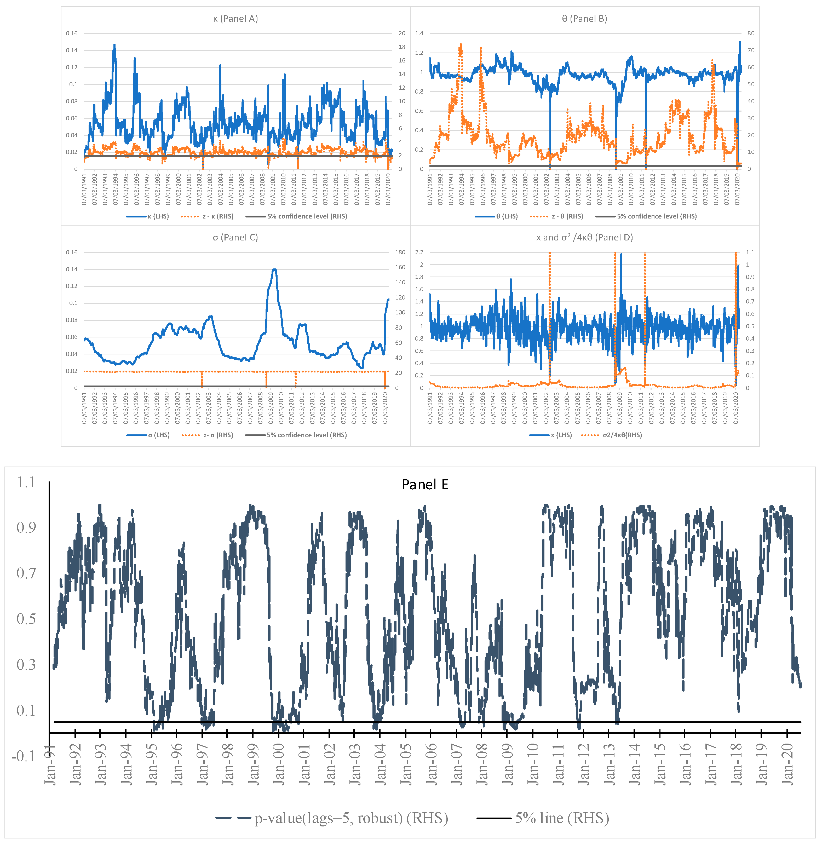
Figure 4.
Estimated Panel A), (Panel B), x Panel C), corresponding z-statistic, and leakage ratio () of Hertz stock price using 2-year rolling window.
Figure 4.
Estimated Panel A), (Panel B), x Panel C), corresponding z-statistic, and leakage ratio () of Hertz stock price using 2-year rolling window.
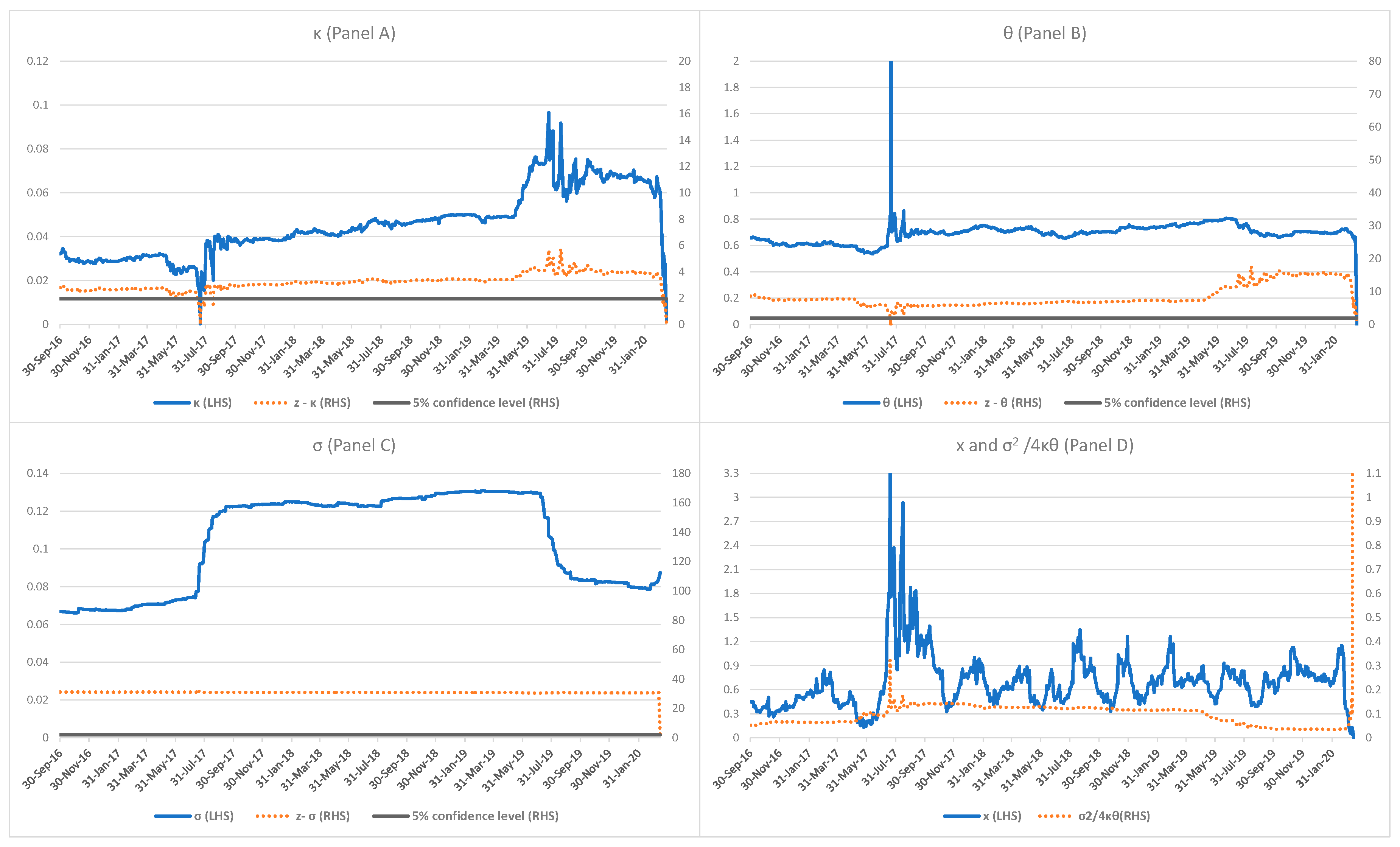
Figure 6.
Estimated Panel A), (Panel B), x Panel C), corresponding z-statistic, and leakage ratio () of GameStop stock price with 50-day moving average using 2-year rolling window.
Figure 6.
Estimated Panel A), (Panel B), x Panel C), corresponding z-statistic, and leakage ratio () of GameStop stock price with 50-day moving average using 2-year rolling window.
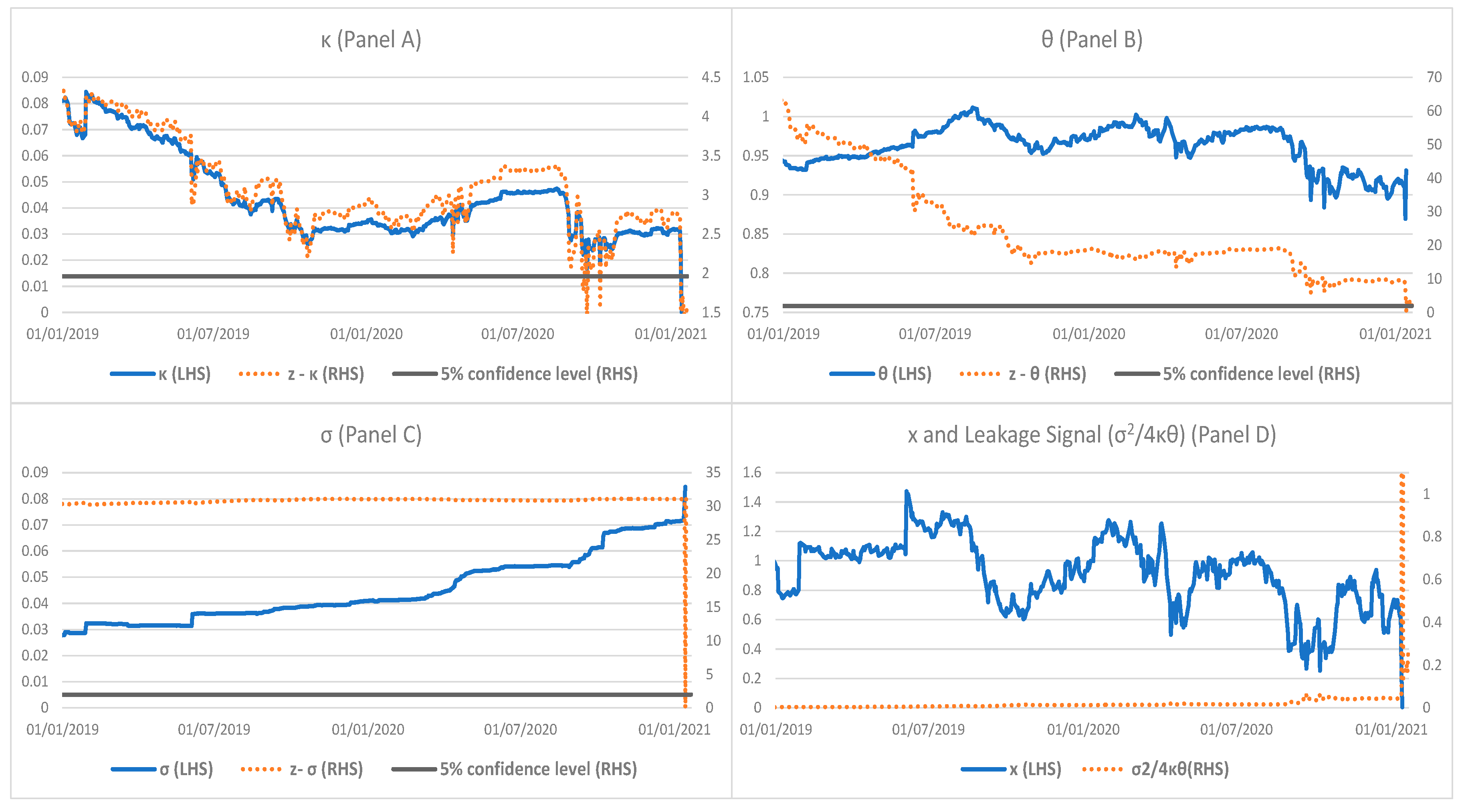
Figure 7.
A simple regression of ln(κ) = a + bln(COVID-19) with t-statistic in parenthesis for Hertz stock price.
Figure 7.
A simple regression of ln(κ) = a + bln(COVID-19) with t-statistic in parenthesis for Hertz stock price.
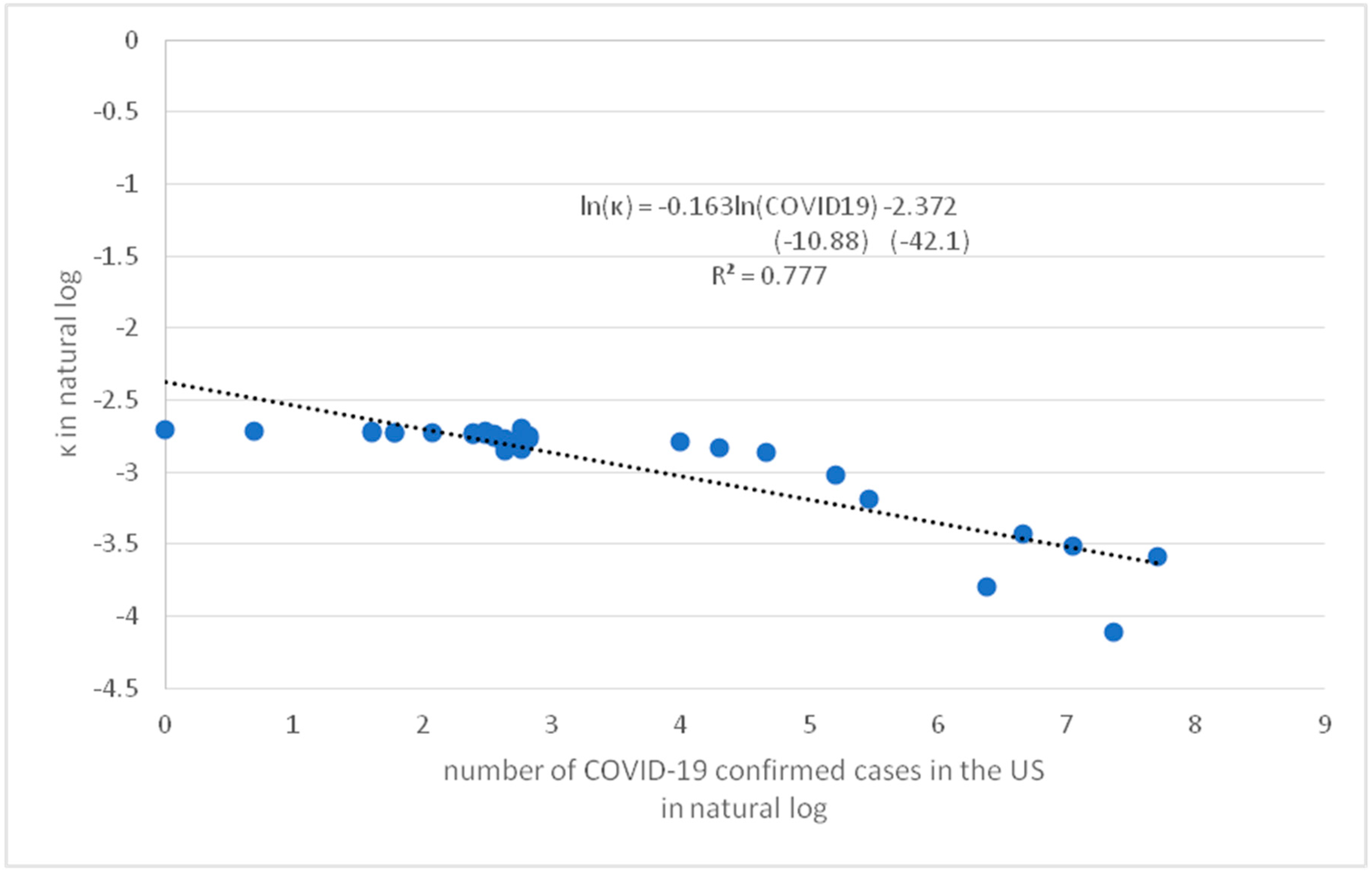
Figure 8.
A simple regression of ln( ) = a + bln(COVID-19) with t-statistic in parenthesis for Hertz stock price.
Figure 8.
A simple regression of ln( ) = a + bln(COVID-19) with t-statistic in parenthesis for Hertz stock price.
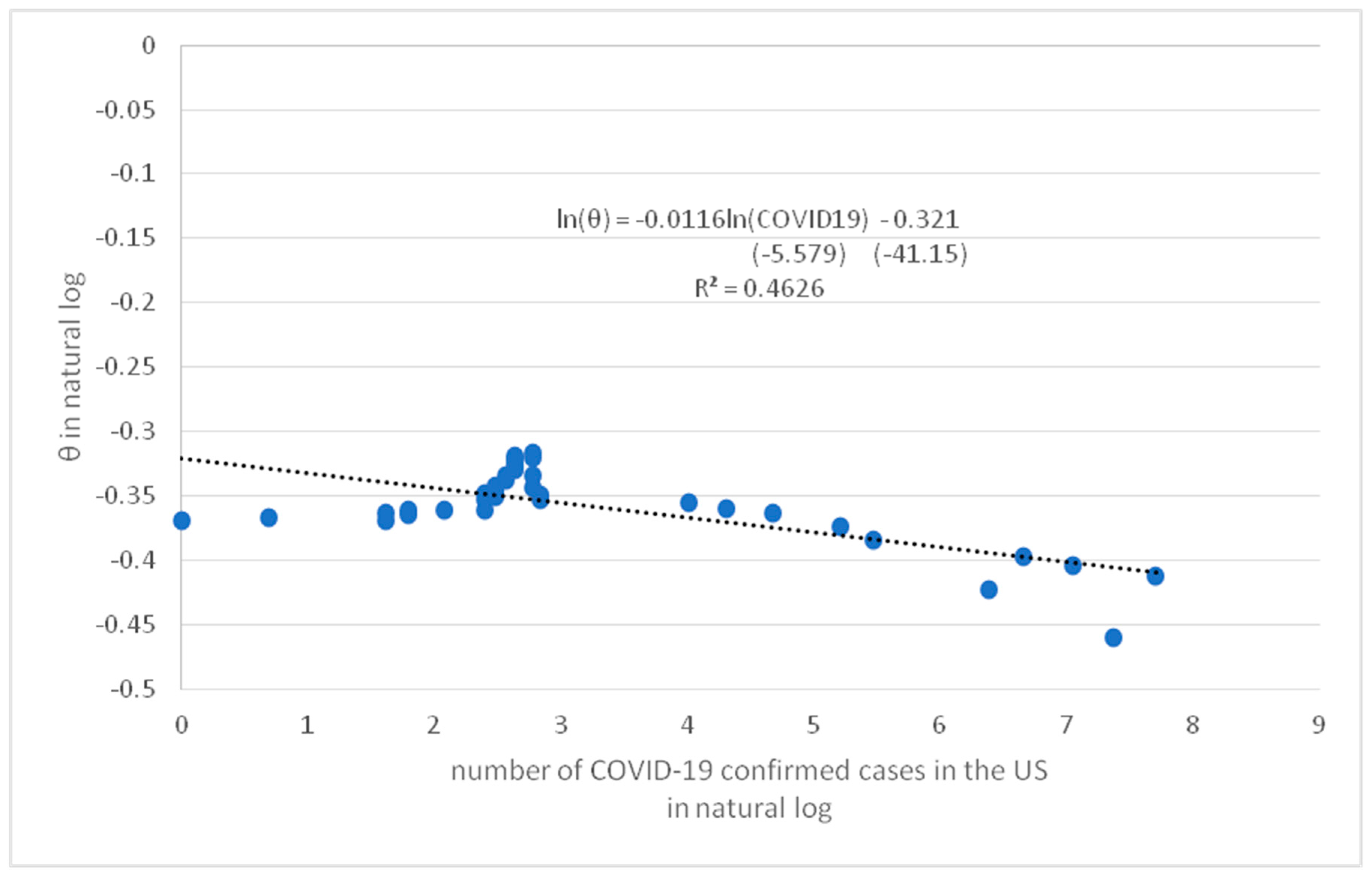
Figure 9.
A simple regression of ln(σx) = a + bln(COVID-19) with t-statistic in parenthesis for Hertz stock price.
Figure 9.
A simple regression of ln(σx) = a + bln(COVID-19) with t-statistic in parenthesis for Hertz stock price.


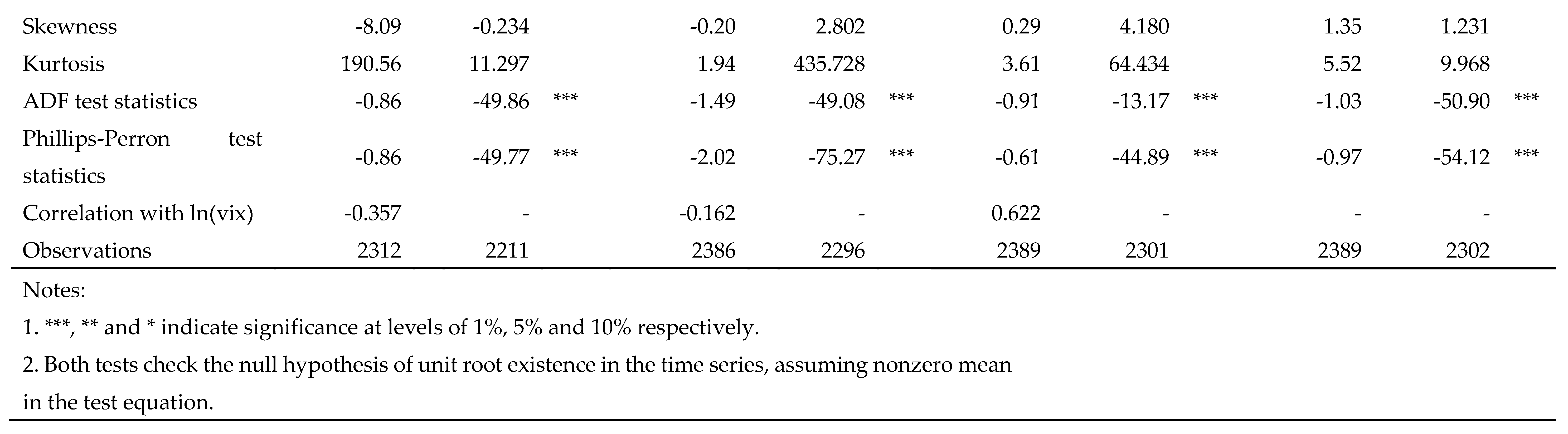
Table 1.
Descriptive statistics of ln(κ), ln(Sθ), ln(σx) for S&P500 Index and ln(VIX).
|
Table 2.
Tests for co-integration of ln(κ), ln(Sθ), ln(σx) for S&P500 Index and ln(VIX).
|
Table 3.
Estimates of long-run coefficient ( for ln(κ), ln(Sθ), ln(σx) for S&P500 Index and ln(VIX).
Table 3.
Estimates of long-run coefficient ( for ln(κ), ln(Sθ), ln(σx) for S&P500 Index and ln(VIX).
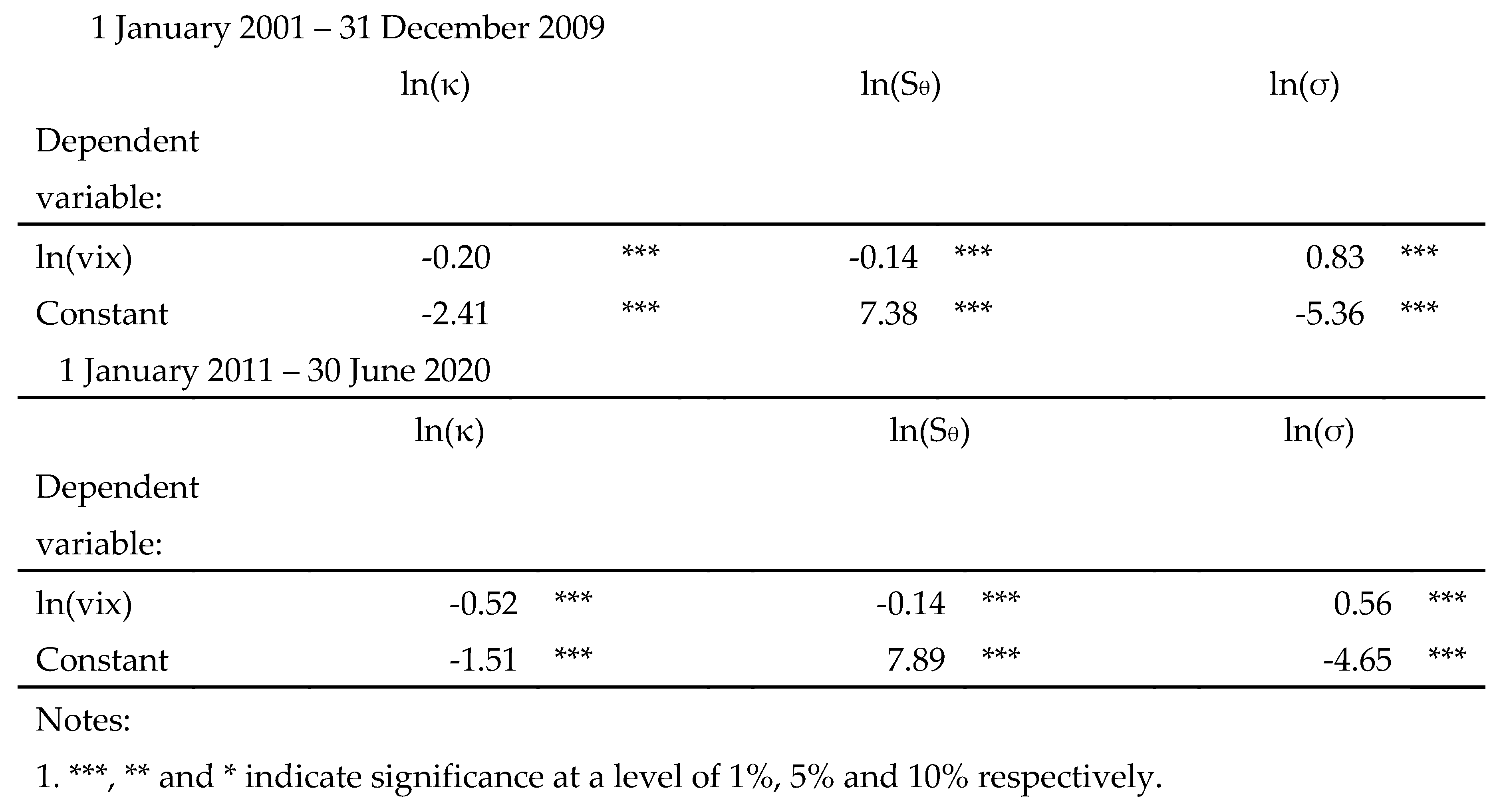 |
Table 4.
Estimation results of the short-run dynamics for ln(κ), ln(Sθ), ln(σx) for S&P500 Index and ln(VIX).
Table 4.
Estimation results of the short-run dynamics for ln(κ), ln(Sθ), ln(σx) for S&P500 Index and ln(VIX).
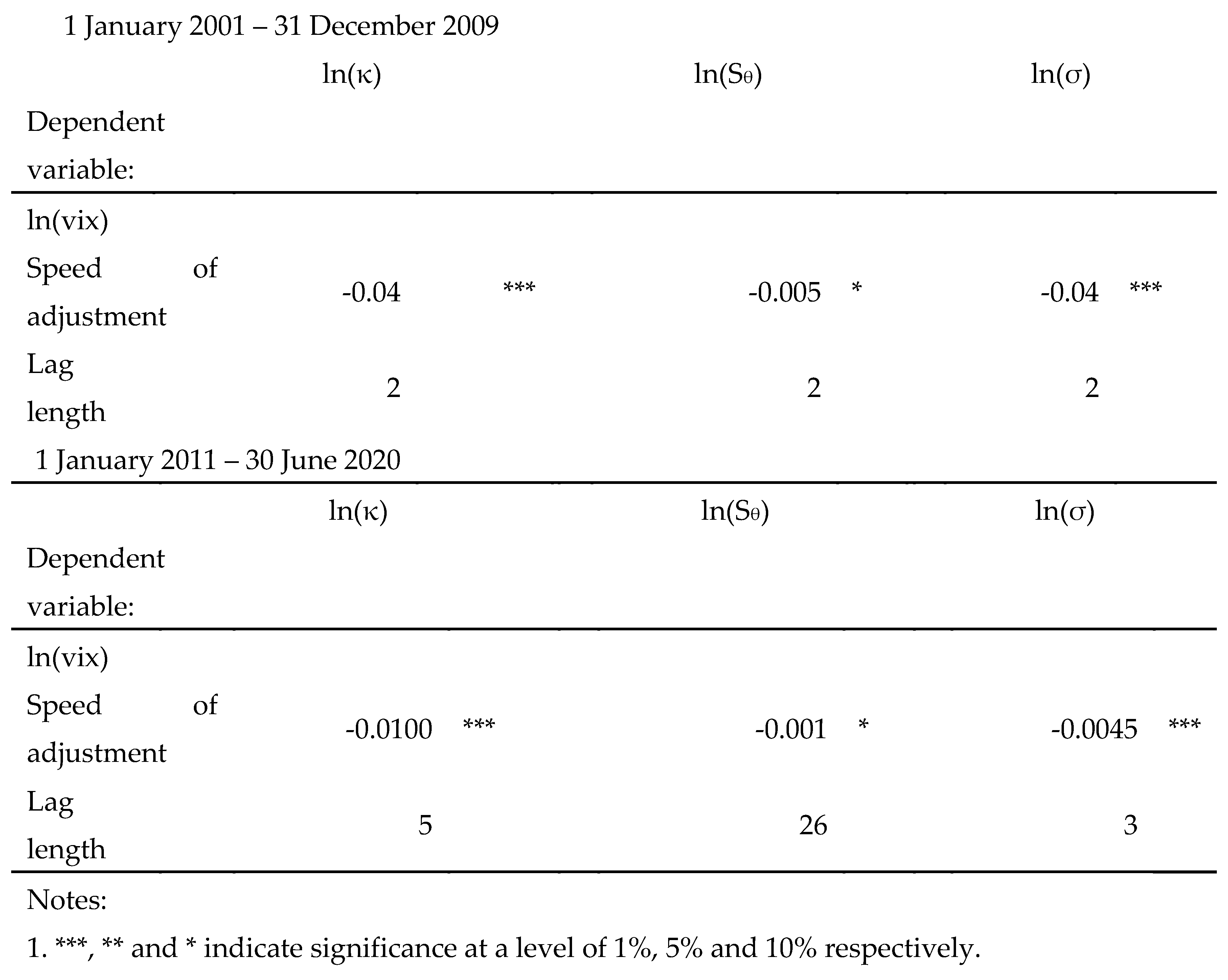 |
Table 5.
Descriptive statistics of , and of GameStop stock price.
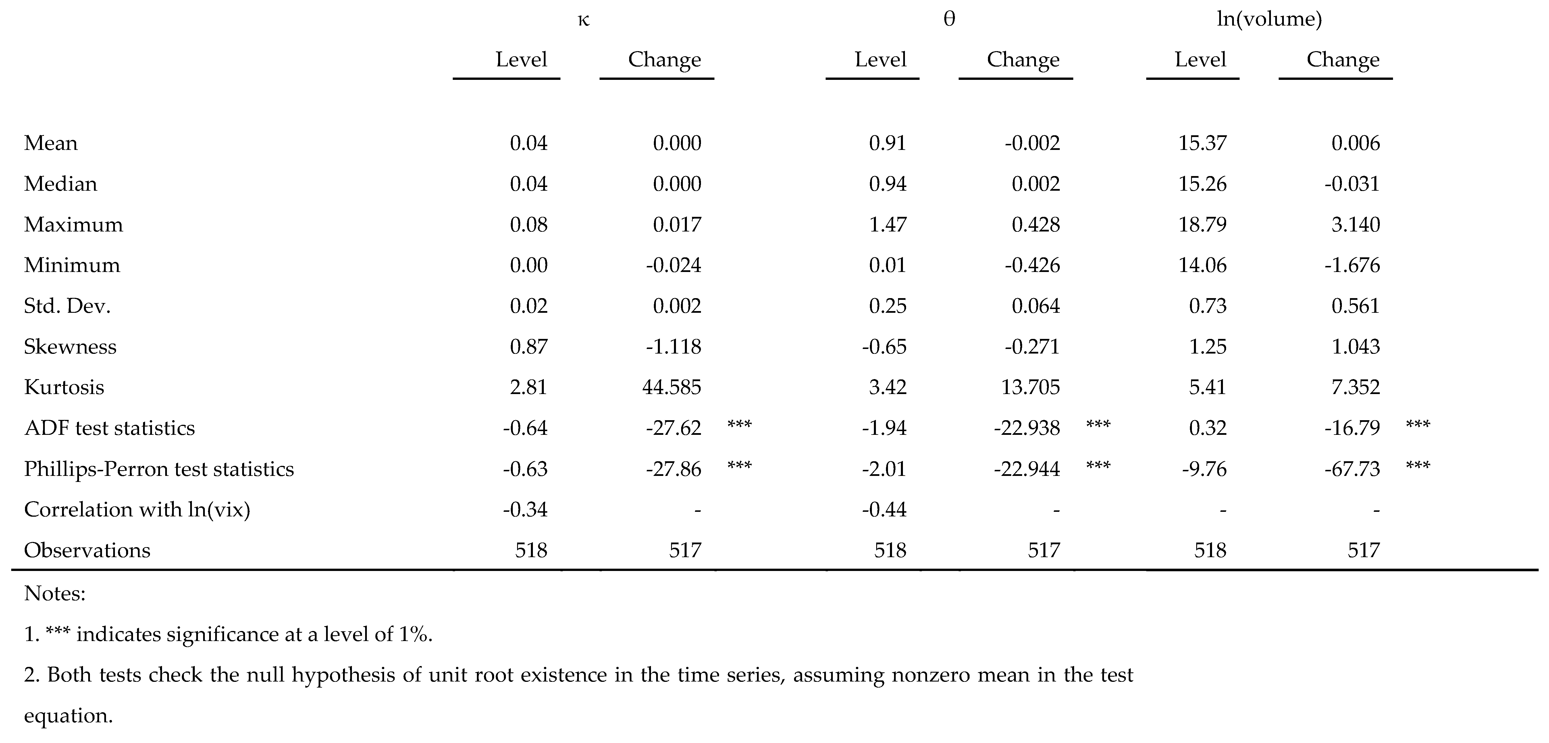 |
Table 6.
Tests for co-integration of , and of GameStop stock price.
|
Table 7.
Estimates of long-run coefficient ( for , and of GameStop stock price.
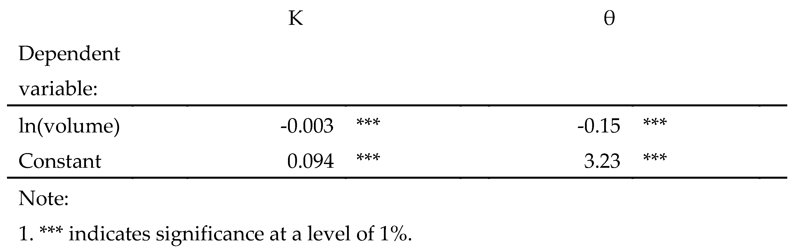 |
Table 8.
Estimation results of the short-run dynamics for , and of GameStop stock price.
 |
Disclaimer/Publisher’s Note: The statements, opinions and data contained in all publications are solely those of the individual author(s) and contributor(s) and not of MDPI and/or the editor(s). MDPI and/or the editor(s) disclaim responsibility for any injury to people or property resulting from any ideas, methods, instructions or products referred to in the content. |
© 2023 by the authors. Licensee MDPI, Basel, Switzerland. This article is an open access article distributed under the terms and conditions of the Creative Commons Attribution (CC BY) license (http://creativecommons.org/licenses/by/4.0/).
Copyright: This open access article is published under a Creative Commons CC BY 4.0 license, which permit the free download, distribution, and reuse, provided that the author and preprint are cited in any reuse.


