Submitted:
06 November 2023
Posted:
07 November 2023
You are already at the latest version
Abstract
Artificial intelligence algorithms have gained widespread adoption in the field of air conditioning load prediction. However, their prediction accuracy is substantially influenced by the quality of training samples. Training samples that lack relevance to the predicted moments can introduce interference into the neural network's learning process, potentially leading to a state of local convergence during its iterative process. This, in turn, diminishes the robustness and generalization capabilities of the prediction model. To enhance the prediction accuracy of air conditioning load prediction models based on artificial intelligence algorithms, this study presents an artificial intelligence algorithm prediction model based on the method of sample similarity sample screening. Initially, the comprehensive similarity coefficient between samples is computed using the gray correlation analysis method, enriched with enhancements in information entropy. Subsequently, a subset of closely related samples is extracted from the original dataset and employed as the training dataset for the artificial intelligence prediction model. Finally, the trained artificial intelligence algorithm prediction model is deployed for air conditioning load prediction. The results illustrate that the method of screening training samples based on sample similarity effectively improves the prediction accuracy of BP neural network (BPNN) and extreme learning machine (ELM) prediction models. However, it is important to note that this approach may not be suitable for genetic algorithm BPNN (GABPNN) and support vector regression (SVR) models.
Keywords:
similarity method
; cooling load prediction
; neural network prediction model
; entropy weight method
; grey correlation method
1. Introduction
The energy consumption of buildings in China accounts for approximately 30% of the total social energy consumption, while in Europe and OECD countries, this figure exceeds 40% [1,2,3]. This substantial energy usage in buildings is a major contributor to global warming, climate change, and air pollution [4]. Among the energy-consuming components of buildings, the air-conditioning system stands out, responsible for 40-60% of the total energy consumption [5,6]. As a result, reducing energy consumption in air-conditioning systems is crucial for the sustainable, low-carbon development of buildings.
Air conditioning load prediction plays a pivotal role in energy system planning and the development of efficient air conditioning system operation strategies. Early-hour-by-hour air conditioning load prediction models were primarily constructed using the transfer function method, which exhibited low prediction accuracy and limited generalization capability. Consequently, numerous researchers have explored alternative prediction models for air conditioning load forecasting. Wang et al. [7] introduced a combined prediction model, demonstrating its superior accuracy and stability compared to previous models. Yun et al. [8] proposed an autoregressive prediction model incorporating exogenous time and temperature indices, achieving prediction accuracy similar to that of the Back Propagation Neural Network (BPNN) model and outperforming traditional autoregressive models. Kwok and Lee [9] presented a probabilistic entropy-based neural network prediction model, incorporating six outdoor meteorological parameters and accounting for dynamic building occupancy factors. Their results highlighted the significant impact of building occupancy factors on cooling load prediction and the improved accuracy of the model when considering these factors. Al-Shammari et al. [10] introduced a support vector machine (SVM) prediction model coupled with a firefly optimization algorithm, surpassing genetic planning and artificial neural network models in prediction accuracy. Sajjadi et al. [11] proposed an extreme learning machine (ELM) prediction model, comparing it with genetic planning and BPNN models in regional short-term heat load prediction, with ELM demonstrating superior accuracy. Leung et al. [12] presented a neural network prediction model utilizing the Levenberg-Marquardt algorithm, incorporating seven types of outdoor meteorological parameters, electricity consumption, and date types of building occupancy space. Their results showed that considering factors such as electricity consumption and building occupancy space type significantly improved prediction accuracy. Ilbeigi et al. [13] developed a trained multi-layer perceptron (MLP) model, incorporating artificial neural networks and genetic algorithms to accurately predict building energy consumption. The proposed model exhibited applicability in predicting and optimizing energy consumption for similar buildings. Fan et al. [14] introduced a short-term cooling load prediction model based on deep learning algorithms, demonstrating the substantial improvement in cooling load prediction through unsupervised deep learning for feature extraction. Duanmu et al. [15] recognized the insufficiency of basic building information in urban planning and introduced a prediction model based on cooling load factors, which yielded a prediction error of less than 20% in general. Yao et al. [16] proposed a combined hour-by-hour cooling load prediction model based on hierarchical analysis, determining weight values for multiple linear regression, autoregressive sliding average, artificial neural network, and gray prediction models through hierarchical analysis. The results indicated that the combined model based on hierarchical analysis achieved higher prediction accuracy than individual models. Ding et al. [17] introduced integrated models combining genetic algorithms with support vector regression (SVR) and wavelet analysis, comparing their effects on short-term and ultra-short-term cooling load predictions. The results showed that the genetic algorithm-SVR model delivered high accuracy for short-term cooling load predictions, while the genetic algorithm-wavelet analysis-SVR model excelled in ultra-short-term cooling load prediction.
Different prediction models each offer their own advantages and disadvantages, and in most cases, their prediction accuracy is deemed acceptable. The linear regression model, while relatively simple, often falls short in delivering satisfactory prediction outcomes. On the other hand, gray box models offer the benefit of not requiring a deep understanding of their internal mechanisms, making their prediction process relatively straightforward. However, the accuracy of these models tends to diminish when dealing with highly discrete data.
While artificial intelligence algorithms have found wide-ranging application in the field of air conditioning load prediction, they are not without their shortcomings. To enhance prediction accuracy, artificial intelligence algorithms frequently demand a significant volume of historical data as training samples. Yet, in practical engineering scenarios, obtaining a sufficient number of effective training samples is often challenging. Moreover, samples that lack relevance to the specific prediction moments can introduce interference into the neural network's training process, potentially leading to local convergence during the iterative process, thereby compromising the model's predictive accuracy.
Hence, focusing on the key factors influencing short-term air conditioning load prediction, this study introduces an artificial intelligence algorithm prediction model for air conditioning cooling load based on sample similarity improvement. The primary objective is to enhance the prediction accuracy of commonly used artificial intelligence algorithms.
Initially, a correlation analysis method is employed to identify the primary factors impacting air conditioning load changes. This aids in reducing the dimensionality of input samples and simplifying the prediction model. Subsequently, the gray correlation analysis method, enhanced with information entropy improvements, is utilized to assess the degree of similarity between samples. The original samples are then preprocessed based on their similarity, eliminating training samples that bear little relevance to the input variables at the prediction moment, and mitigating the interference of anomalous samples during the training and learning processes of artificial intelligence algorithms. Finally, this refined set of training samples is integrated into the standard artificial intelligence algorithm prediction model, thereby elevating the model's predictive accuracy.
The rest of this paper is organized as follows. In Section 2, the conventional artificial intelligence algorithm prediction model and the improved prediction processes are described in detail. In Section 3, a case building located in Tianjin is introduced to evaluate the performance of the improved method. Finally, conclusions and the possible future works are provided in Section 4.
2. Methodologies
2.1. Air Conditioning load prediction model based on conventional artificial intelligence algorithm
2.2.1. BPNN prediction model
The BPNN is a multi-layer feed-forward neural network that relies on error back-propagation. It is widely recognized as a quintessential supervised learning algorithm. This neural network model employs non-linear transfer functions, enabling neurons in each hidden layer to acquire the capacity to learn. Throughout the training process of the network, it utilizes the gradient descent learning rule, which facilitates the minimization of global error, ultimately aiming to attain the optimal expected value. In instances where the training error fails to meet the predefined accuracy criteria, the weights and thresholds of each neuron are iteratively adjusted through backpropagation, starting from the output layer and progressing towards the input layer, until the output error aligns with the specified accuracy threshold.
The structure of a typical three-layer (single hidden layer) BPNN is shown in Figure 1.
As illustrated in Figure 1, a typical three-layer BPNN typically comprises an input layer, a hidden layer, and an output layer, with interconnected neurons extending from one layer to the next (from the input layer to the hidden layer and from the hidden layer to the output layer). Neurons within the same layer, however, are not interconnected.
The quantity of neurons in the hidden layer, situated between the input and output layers, is typically determined based on the structural characteristics of the input samples. The formula for calculating the number of neurons in the hidden layer is expressed in Eq. (1) [18,19]:
Here, l is Number of neurons in the hidden layer, and p is number of neurons in the input layer.
The learning process of BPNN is shown in Figure 2.
Evidently, as illustrated in Figure 2, the learning process of Backpropagation (BP) neural networks typically involves the following stages [19,20,21,22]:
In the first step, the initial connection weights and thresholds for the BPNN are randomly assigned within the range of [-0.5, 0.5] as part of the network's initialization process.
In the second step, the output values of the neurons in the hidden layer are calculated using specific computational expressions, as detailed in Equations (2) and (3):
Here, Sj is the input signal of the hidden layer neuron, Hj is output value of the hidden layer neuron, xt is the input variable, ωjt is the connection weights of neurons between the input layer and the hidden layer, αj is the threshold value of the neuron in the hidden layer, and F(S) is the transfer function of the hidden layer neuron.
In the third step, the output values of the neurons in the output layer are computed using the computational expressions detailed in Equations (4) and (5):
Here Sk is the input signal of the output layer neuron, Ok is the output value of the output layer neuron, ψkj is the connection weights of the neurons between the hidden layer and the output layer, βk is the threshold value of the output layer neuron, and G(S) is the transfer function of the output layer neuron.
In the fourth step, the error between the output value of a single training sample network and the desired output value is computed as indicated in Equation (6):
Here, ek is computational error of a single training sample, and Ek is the desired output value of the BPNN.
In the fifth step, the connection weights and thresholds of the neurons in the hidden and output layers are updated, as demonstrated in Equations (7) to (10):
Here, η is the learning efficiency of the neural network, δj is the partial derivative of the computational error function with respect to the connection weights between neurons in the input and hidden layers, δk is the partial derivative of the computational error with respect to the connection weights between the neurons of the hidden and output layers, and μ is the additional momentum coefficient.
In the sixth step, the global error is computed as indicated in Equation (11):
Here, eall is global error of BPNN, and m is total number of training samples.
In the seventh step, it is determined whether the global error of the BPNN meets the set requirements. If the error requirements are satisfied, the iteration ends, and the prediction results are output. If the error requirements are not met, the process returns to the second step for the next round of learning.
2.2.2. Genetic algorithm BPNN prediction model
BPNN employs the gradient descent learning rule to minimize global error, while it still exhibits issues including limited model robustness, slow learning and convergence rates, and susceptibility to local minima during the learning process. Moreover, the choice of initial connection weights and thresholds significantly influences the training of BPNN. The utilization of genetic algorithms for optimizing the learning process of BPNN can mitigate these concerns to a considerable extent [18]. Thus, genetic algorithm BPNN (GABPNN) prediction model is generally used to replace the BPNN model for prediction.
The genetic algorithm is a global optimization search technique inspired by Darwin's principle of "survival of the fittest" in the biological world. Unlike methods that rely on function derivatives and continuity, genetic algorithms offer a unique approach. They encode relevant parameters into a set of chromosomes and employ probabilistic methods for a sequence of iterative operations, including chromosome selection, crossover, and mutation. This process culminates in the retention of individuals with high fitness and the elimination of those with low fitness. Through this procedure, the offspring inherit information from their parent individuals and, simultaneously, adapt more effectively to their environment. This results in the optimization of the entire population [18,23,24,25].
The learning process of the GABPNN is depicted in Figure 3.
As depicted in Figure 3, the learning process of the GABPNN primarily comprises the following three phases: Initially, the network's topology is determined, and the initial population for the genetic algorithm is generated. Subsequently, the genetic algorithm is employed to optimize the initial connection weights and thresholds of the BPNN. In the final step, the optimal weights and thresholds obtained in the preceding phase are assigned to the BPNN for training and learning. The concrete steps of the genetic algorithm are shown below [13,18,19,23,24,25]:
The first step is population initialization. Population initialization entails the derivation of the initial solutions for the population in accordance with predefined encoding protocols. Genetic algorithms, by their intrinsic nature, are not equipped to interface directly with parameters inherent to the problem space. Thus, these parameters necessitate transformation into chromosomes or individuals within the genetic space, achieved through the encoding process. Prevalent encoding methodologies encompass programming encoding, multilevel parameter encoding, character encoding, structured encoding, floating-point encoding, Gray encoding, and binary encoding. Among these methodologies, binary encoding holds wider application within genetic algorithms. This modality typically leverages 0 and 1 characters to shape the genotype string data within the genetic space. When optimizing the initial connection weights and thresholds of the BPNN via a genetic algorithm, each constituent within the population typically embodies the encoding for the connection weights linking the input layer with the hidden layer, the threshold governing the hidden layer, the connection weights interconnecting the hidden layer and the output layer, and the threshold dictating the output layer.
The second step is the calculation of the fitness function. The fitness of an individual within the population serves as the metric by which its quality is assessed. A greater fitness value corresponds to heightened adaptability and overall superiority. The formulation of an individual's fitness function is conventionally expressed in the manner delineated by Eq. (12):
Here, F is the individual fitness value.
The third step is the selection operation. The objective of this operation is to emulate the natural course of evolution by singling out the most adept individuals from the population while eliminating those with diminished fitness. This ensures that the genes of the most optimized individuals can be inherited through direct or indirect modes. Common methodologies for genetic algorithm selection operations encompass the roulette method, the tournament method, and random traversal approaches. The roulette method is especially ubiquitous, with individual selection probabilities being directly proportional to their fitness values. The calculation of the probability of individual l being selected is explicated in Eq. (13):
Here, Pl is the probability of individual l being selected, Fl is the fitness value of individual ,and n is the number of populations, individuals.
Eq. (13) elucidates that an individual boasting a heightened fitness value enjoys an augmented likelihood of selection within the population.
The fourth step is the crossover operation. This operation involves the stochastic selection of two parental individuals from the population and the subsequent recombination of select chromosomes to generate a novel individual. The raison d'être of this operation is to expedite the search capability of the genetic algorithm through chromosome crossovers among individuals of superior quality. Diverse methodologies for crossover operations exist. As individuals in the population are encoded as real numbers, the adoption of real number crossover techniques is frequently the norm. Mathematically, this process is expounded in Eqs. (14) and (15).
Here, aqt, ast is the new chromosome of the qth chromosome aq and the sth chromosome as recombined by crossover at the t position, and b is the random number with values in the range [0, 1].
The fifth step is the mutation operation. This operation primarily seeks to replicate the diversity present in populations during the course of biological evolution. The modus operandi involves the selection of a specific individual within the population and the alteration of a gene within the gene sequence of this individual, effecting the creation of a more proficient individual. The data representation of the mutation process pertaining to the t-th gene of the q-th individual, Xqt, is elucidated in Eqs. (16) and (17):
Here, c is the random number, taking values in the range [0, 1], d is current iteration number, d is maximum number of evolution, X'qt is mutated gene, Xmax is the upper bound of gene Xqt, Xmin is the lower bound of gene Xqt, and r is random number with values in the range [0, 1].
The sixth step is to determine whether the evolution is terminated or not. Termination is effected when the training error (fitness) of the network satisfies pre-established prerequisites or when the maximum number of iterations is reached. At this juncture, the iterative decoding process concludes, yielding the optimal weights and thresholds, thereby marking the culmination of the evolutionary process. In the event that these termination conditions remain unmet, the process reverts to the third stage, subsequently iterating the computational process until the stipulated termination criteria are met.
2.2.3. SVR prediction model
The SVM, introduced by American scholars Cortes and Vapnik in 1995 [26], is a learning algorithm devised to address the challenge of classifying two datasets. This approach entails transforming the non-linear classification problem associated with sample data into a linear classification problem, achieving this through the mapping of the sample data into a high-dimensional space. Subsequently, Vapnik introduced the ε linear insensitive loss function, paving the way for the development of a real-valued SVM, commonly known as a SVR learning machine [27].
The architecture of the SVR learning machine is shown in Figure 4.
Evidently, as depicted in Figure 4, the input and output layers of the SVR learning machine are interconnected through kernel function nodes. Each kernel function node corresponds to a support vector, and the linear combination of these kernel function nodes forms the output of the SVR learning machine.
Assuming a total of m training samples, the input and output sample sets of the training samples are (xi is the input column vector of the sample;yi is the output value of the sample,;),then e input and output values of the training samples are linear in the high dimensional space as shown in Eq. (18) [27]:
Here, g(x) is the output value (the predicted value) of the SVR model, φ(x) is the nonlinear mapping function, V is the weight vector, and v is the linear regression coefficient (intercept).
The specific expression of the ε linear insensitive loss function is shown in Eq. (19):
Here, Lε(g(x), y) is the ε linear insensitive loss function, and ε is the error requirement for the linear regression function.
From Eq. (19), it can be seen that the smaller value of ε indicates the smaller error.
From Eq. (19), when the difference between the predicted and actual values of the SVR model is less than or equal to ε, the value of loss is zero.
The weight vector V and the regression coefficients v are calculated using the regularized risk function as shown in Eq. (20):
Here, C is the penalty factor, which indicates the degree of punishment for training errors larger than ε. The larger the C indicator, the stronger the punishment, and ξi, ξi* are the slack variables.
By introducing the Lagrangian function and performing a pairwise transformation, the solution to Eq. (20) can be converted to the solution to Eq. (21).
Here, , are the Lagrange multipliers, and is the kernel function and .
The more widely used kernel functions are the linear kernel function, the high order polynomial kernel function, the radial basis kernel function and the Sigmoid kernel function.
The results of solving Eq. (21) can be brought into Eq. (18) to find the SVR function as shown in Eq. (22):
2.2.4. ELM prediction model
Traditional feedforward neural networks with a single hidden layer have found widespread application in engineering. Nonetheless, certain issues persist. For instance, these neural networks commonly employ the gradient descent learning rule, a process that involves iterative optimization searches during training. This approach leads to slower training and learning, and it can often result in the network becoming trapped in a locally optimal state. In response to these challenges, Huang et al. [28], affiliated with Nanyang Technological University in Singapore, introduced a novel single hidden layer feedforward neural network known as the "ELM" in 2004. This innovative algorithm obviates the need for adjusting connection weights and thresholds within the neural network according to the gradient descent learning rule during the training and learning process. Instead, it merely necessitates the specification of the number of neurons in the hidden layer and the selection of an infinitely differentiable hidden layer transfer function. By doing so, the optimal solution for the neural network can be attained. Subsequently, Huang et al. [29] conducted a comprehensive investigation into the principles and application efficacy of the ELM. Their findings reveal that, when compared to conventional feedforward neural networks, the ELM not only demonstrates superior generalization capabilities but also exhibits a faster learning rate.
In making prediction using the ELM, it is also assumed that there are a total of m training samples, and the input and output sample sets of the training samples are (xi is the input column vector of the sample. ; yi is the output vector of the sample. ;), a linear function is used for the transfer function of the neurons in the output layer.
The structural diagram of the ELM is similar to that of a typical three-layer BPNN (shown in Figure 1), and the expression for the calculation of the output value of the output layer of the neural network is calculated by Eq. (23):
Here, Oi is the vector of output values of the neural network output layer, ,ωj is the weight vector between the jth hidden layer and the neurons of the input layer, , and ψj is the weight vector between the jth hidden layer and the output layer neuron, .
Assuming the existence of αj, ωj and ψj that make infinitely close to
zero, then Eq. (23) can be converted to Eq. (24):
The matrix expression for m training samples is shown in Eq. (25):
Here, B is the weight matrix between the neurons of the hidden and output layers of all training samples, Z is the output value matrix of the neurons of the hidden layer of all training samples, and T is the output value matrix of the neurons of the output layer of all training samples.
Mathematical expressions for matrices B, Z and T are shown in Eqs. (26), (27) and (28), respectively:
After a series of studies, Huang et al. have proved the following two theorems [29]:(1) For any m different training samples(here,,), if the transfer function of the hidden layer is infinitely differentiable in any interval, then for a single-layer feedforward neural network with m hidden-layer neurons, at any assignment to ωj and αj (here,,), The matrix Z is invertible and ,(2) For any m different training samples (here,,), given an arbitrarily small value of error ε(), if the transfer function of the hidden layer is infinitely differentiable in any interval, then for a single-layer feedforward neural network with M () hidden-layer neurons, there is for any assignment to ωj and αj (here,,). Therefore, the ELM algorithm transforms the problem of finding the optimal connection weights between the input and hidden layers, the connection weights between the hidden and output layers, and the hidden layer threshold into the problem of finding the optimal connection weights between the hidden and output layers.
Through the training and learning process of the ELM, wherein values of αj and ωj are randomly assigned while maintaining the magnitude of these two parameters constant, the connection weight matrix B connecting the neurons of the hidden layer to the output layer can be derived. This is achieved by solving Eq. (29) utilizing the least squares method.
By solving Eq. (29), the solution of the weight matrix:
Here, Z+ is the Moore-Penrose generalized inverse of the hidden layer output matrix Z of the ELM.
The exact procedure of the ELM algorithm is as follows [29]:
In the first step, the input and output variables for the ELM are determined based on the characteristics of the sample data. The number of hidden layer neurons, denoted as l, is determined according to the number of input variables. Concurrently, an infinitely differentiable transfer function F(S) is selected for the hidden layer neurons.
In the second step, arbitrary values are assigned for the connection weights that link the input layer to the hidden layer neurons, as well as the thresholds for the hidden layer neurons.
In the third step, the output matrix Z for the hidden layer neurons is computed.
In the fourth step, the connection weight matrix B between the hidden layer and the output layer neurons is computed.
2.2. Improved air conditioning load prediction model based on similarity
2.2.1. Calculation of comprehensive similarity coefficient
To quantify the similarity between predicted and historical moments of model input variables, this study introduces the concept of a comprehensive similarity coefficient. Unlike the traditional correlation coefficient, the comprehensive similarity coefficient considers the unique contributions of individual input variables to the overall similarity of the samples. This approach provides a more objective and comprehensive assessment of sample similarity. The calculation of this comprehensive similarity coefficient is based on a combination of the gray correlation method and information entropy, enhancing the rigor and comprehensiveness of the similarity assessment.
(1) Grey correlation analysis method
The Gray correlation analysis method, established upon the foundational principles of the gray system theory pioneered by Professor Deng, leverages the gray correlation degree to furnish a quantitative framework for appraising the dynamic evolution of a system. This methodology is particularly well-suited for the analysis of dynamic processes, distinguishing itself from other methods. In the context of computing the comprehensive similarity coefficient, this study introduces an enhanced Gray correlation analysis method that incorporates information entropy. The detailed computational procedure for determining the comprehensive similarity coefficient is delineated in Figure 5. This refined approach enhances the scholarly rigor and precision of the system's transformation analysis.
As can be seen in Figure 5, the main steps in calculating the comprehensive similarity coefficient are:
In the first step, the feature vectors of the input samples of the building cooling load prediction moments and historical moments are first determined, as shown in Eq. (31):
Here, x is the input sample feature vector, b is the input variable eigenvalue, t is the number of input variables, and h is the hth moment, h=0, 1, 2, ..., n, when h=0, it means the prediction moment, when h≠0, it means the historical moment.
The feature vectors of the input samples from the predicted and historical moments are utilized to form the feature matrix A as in Eq. (32):
Here, A is the feature matrix of the input sample.
In order to ensure the reliability of the analysis and to make the eigenvalues of different input variables comparable, this study maps the eigenvalues of the input variables to the range of [0, 1], which is pre-processed by dimensionless and normalization as shown in Eq. (33):
Here, is the eigenvalue of the input variable after dimensionless processing, is the minimum value of the predicted versus historical moment at the tth input variable eigenvalue, and is the maximum value of the predicted versus historical moment at the tth input variable eigenvalue.
The normalization of matrix A using Eq. (33) yields the normalized matrix A′ as shown in Eq. (34):
Here, A′ is the feature matrix of the normalized input sample.
In the second step, the difference between the predicted moment and the hth historical moment in the eigenvalue of the tth input variable is calculated as shown in Eq. (35):
In the third step, the similarity between the predicted moment and the hth historical moment sample in terms of the tth input variable eigenvalue is calculated as shown in Eq. (36):
Here, is the first minimum difference, is the second minimum difference, is the first maximum difference, is the second maximum difference, and ρ is the resolution coefficient.
In the fourth step, the comprehensive similarity coefficient between the predicted moment and the input sample of the hth historical moment is calculated, as shown in Eq. (37):
Here, rh is the comprehensive similarity coefficient and Wt is the weight value of the tth input variable.
It can be seen from Eq. (36), when is maller, is large. In other words, when the difference between the predicted moment and the h-th historical moment in the characteristic value of the t-th input variable is smaller, the similarity between the predicted moment and the historical moment in the t-th input variable is greater. Eq. (37) reveals that a larger comprehensive similarity coefficient rh signifies a stronger similarity in the composite characteristics between the predicted moment and the historical moment input samples. Moreover, it is evident that the magnitude of the input variable weight values also impacts the selection of similar samples.
(2) Determination of weight values for different input variables
The methods for determining the weights of evaluation indicators are generally classified into two categories [30]. The first is the subjective weighting method, where subjective factors hold a greater influence, and decision-makers assign weights based on their experiential judgment. The second is the objective weighting method, which exclusively relies on objective data and derives weights through the extraction and analysis of objective information inherent in the statistical data.
The term "entropy" in the entropy weight method originally finds its roots in thermodynamics, where it serves as a measure of information disorder within a system. In 1948, Shannon [31] introduced the concept of entropy into information theory, labeling it as information entropy. The fundamental principle underpinning decision-making or measurement using information entropy is as follows: the smaller the information entropy associated with an indicator, the greater the information it contributes to the comprehensive evaluation, and consequently, the higher the weight it receives. It is this principle that makes information entropy a valuable tool for gauging the amount of pertinent information contained within data. As a result, it has found extensive application in engineering technology and socio-economic domains. In the practical application of the entropy weight method, the initial step involves computing the information entropy of each parameter based on its degree of variation, followed by the computation of the entropy weight associated with each parameter. The entropy weight method is an objective assignment approach that exclusively relies on the degree of variation in objective factors. This circumvents the subjective influence introduced by decision-makers when determining weight values, resulting in a more objective assignment of indicator weights [32]. Given these advantages, the present study employs the entropy weighting method to determine the weight values for the input variables within the prediction model.
The expression for calculating the information entropy of the tth input variable, as shown in Eq. (38):
Here, Et is the entropy value of the tth meteorological parameter, Pht is the probability of occurrence of the tth input variable in the hth historical day and σ is the moderating coefficient,.
The expression for calculating the probability of occurrence of the tth input variable in the hth historical day is shown in (39):
The formula for the entropy weight of the tth input variable, shown in (40):
2.2.2. Air conditioning load prediction process based on similarity improvement
The prediction process of the enhanced artificial intelligence algorithm model, which relies on sample similarity, is depicted in Figure 6.
Figure 6 outlines the key steps within the prediction process of the improved artificial intelligence algorithm based on sample similarity. These steps are as follows:
In the first step, the primary factors that influence changes in air-conditioning load are identified through a quantitative correlation analysis.
In the second step, a new matrix is constructed using the eigenvectors of the primary influencing factors of air-conditioning load at predicted and historical moments. Comprehensive similarity coefficients for these primary influencing factors at both moments are computed using Eq. (37).
In the third step, a target value for the comprehensive similarity coefficients is established. A subset of similarity samples is then selected from the original sample set, serving as training data for the artificial intelligence prediction model.
In the final step, the trained prediction model, utilizing the artificial intelligence algorithm, forecasts the air-conditioning load.
2.3. Uncertainty calculation
Measurement uncertainty, a non-negative parameter, serves to quantify the dispersion attributed to the measured value based on the available information. It is commonly employed to gauge the dependability of test outcomes. Without this evaluative metric, the results of measurements would lack the means for comparison with other pertinent data, as dictated by the established criteria. Consequently, the assessment of uncertainty in test results assumes a central role as the primary unifying criterion for data quality [33]. To appraise the dependability of test results, a number of researchers have also adopted relative uncertainty analysis in place of traditional uncertainty analysis [34,35,36,37].
According to the basic principle of error propagation, the relative uncertainties of measured and calculated parameters can be calculated according to Eqs. (41)~(43) [38,39]:
Here, εXl is the uncertainty of the measured parameter, A is the half-width of the interval of the measured value, k is the inclusion factor, Xl is the test parameter, ∆εXl is the relative uncertainty of the test parameter, ∆εU is the relative uncertainty of the computed parameter, and U is the series function of the test parameter, U = U(X1, X2, ..., Xn).
3. Results and discussions
3.1. Building cooling load testing case study
The case building is a six-story retro-fitted office building with a total floor area of 5700m2 located in Tianjin, China. The air conditioning area is approximately 4735m2. A ground coupled heat pump system is used to maintain indoor thermal comfort in summer and winter. The ground coupled heat pump system consists of two parallel heat pumps. The nominal cooling/heating capacity of heat pump A is 212kW/213kW, corresponding with a nominal electricity consumption of 40.2kW/48.6kW. The nominal cooling/heating capacity of heat pump B is 140kW/142kW, corresponding with a nominal electricity consumption of 24.2kW/28.5kW. The supply/return water temperatures of heat pump A and B during the cooling season are 7/12℃ and 14/19℃, respectively. The supply/return water temperatures of heat pump A and B during the heating season are 40/35℃. The test mainly focused on weekdays from 9:00 to 17:00 from May 17 to August 19, 2016, with a time interval of 0.5 h. Among them, the low-temperature water in the buried pipe was mainly concentrated in the mode of directly supplying cooling to the building from May 17 to June 20, 2016, and the heat pump units A and B were mainly concentrated in the mode of directly supplying cooling to the building from June 21 to August 19, 2016, respectively. Due to the frequent starting and stopping of the soil source heat pump system on August 19, the data on that date was abnormal and was excluded. In the end, the valid data for the test was from May 17 to August 18, 2016. The main test parameters were air conditioning system supply and return water temperature, flow rate, indoor temperature, and outdoor meteorological temperature.
When assessing the prediction accuracy of the model, this study omits the building's intrinsic thermal storage capacity and makes the assumption that the measured instantaneous cooling supply from the heat pump system accurately represents the instantaneous cooling load of the test building. The expression for computing the cooling supply of the heat pump system is presented in Eq. (44):
Here, Qc (kW) is the cold load of the heat pump system, cpw (kJ/(kg·℃)) is the specific heat capacity of the chilled water, ρw (kg/m3) is the density of the chilled water, Tre (℃) is the return water temperature of the heat pump system, and Tsu (℃) is the water supply temperature of the heat pump system.
The detailed parameters of the test instrument (component), as shown in Table 1.
Testing and the relative uncertainties of the calculated parameters, as shown in Table 2.
As can be seen from Table 2, the relative uncertainties of the tested and calculated parameters are within acceptable limits, so the tested and calculated data are highly reliable [32]. The variation curves of outdoor temperature (To) and relative humidity (RHo) during the test period are shown in Figure 7.
Observing Figure 7, it becomes evident that outdoor temperatures from May 17 to June 20 predominantly ranged between 25.7 and 31.2°C. During this period, relative humidity levels were primarily within the range of 27.0 to 48.0%. The respective averages for these conditions were 28.8°C and 40.2%. In contrast, the period from June 21 to August 18 saw outdoor temperatures mainly falling between 28.9 and 33.7°C. During this timeframe, relative humidity levels were primarily within the range of 51.0 to 73.5%. The respective averages for these conditions were 31.2°C and 62.9%.
The graphs in Figure 8 illustrate the variation curves for outdoor solar radiation intensity (Io) and outdoor wind speed (Vo) throughout the test period.
Figure 8 provides an overview of the solar radiation intensity and outdoor wind speed during the test period. From May 17 to June 20, solar radiation intensity ranged predominantly between 250.5 and 657.0 W/m², with outdoor wind speed mainly within the range of 0.5 to 1.5 m/s. The respective averages for these conditions were 455.8 W/m² and 1.1 m/s. Subsequently, during the period from June 21 to August 18, solar radiation intensity was primarily distributed between 173.0 and 495.0 W/m², while outdoor wind speed predominantly ranged between 0.3 and 1.0 m/s. The respective averages for these conditions were 347.5 W/m² and 0.7 m/s.
Upon comparison, it becomes evident that the average values of outdoor meteorological parameters, which encompass outdoor temperature, relative humidity, solar radiation intensity, and wind speed, significantly differ between the two measurement phases—May 17 to June 20 and June 21 to August 18. This discrepancy underscores the varying impact of outdoor temperature, relative humidity, solar radiation intensity, and wind speed on the cooling load of the building during different stages of the cooling supply. For the sake of clarity, this study refers to the two test phases as the early and middle stages of cooling, respectively.
The building cooling load distribution during the test period, is shown in Figs. 9, 10 and 11, respectively.
Figure 9, Figure 10 and Figure 11 illustrate that the measured cooling capacity of the heat pump system during the middle of the cooling period primarily falls within the range of 62.8 to 80.2 kW, with an average value of 73.4 kW. However, when the active cooling mode is activated during this period, the measured cooling capacity of the heat pump system predominantly ranges between 123.0 and 172.4 kW, with an average value of 161.4 kW.
The variation curves of indoor temperature (Ti) and relative humidity (RHi) at the early and middle stages of cooling are shown in Figure 12 and Figure 13.
Figure 12 illustrates that during the early stage of cooling, the indoor temperature exhibits a minimum of 24.1°C, a maximum of 28.5°C, and a maximum fluctuation of 4.4°C. The indoor temperature is predominantly distributed between 26.0°C and 27.0°C, while relative humidity ranges mainly from 30% to 60%. The average values for these conditions are 26.6°C and 43.3%, respectively. In contrast, as indicated in Figure 13, during the middle period of cooling, the indoor temperature shows a minimum of 23.8°C and a maximum of 26.1°C, with a maximum fluctuation of 2.3°C. The indoor temperature is primarily distributed between 24.8°C and 25.3°C, while relative humidity is mainly distributed between 64% and 73%. The average values for these conditions are 25.1°C and 68.0%, respectively.
This study aimed to assess the prediction accuracy of the model by splitting the measured data into two distinct sets: the training sample set and the test sample set. The building cooling loads from May 17 to June 9 and from June 21 to August 2 were employed as the training samples for the early and mid-measurement models of cooling, while the building cooling loads from June 10 to June 20 and from August 3 to August 18 served as the test samples for the early and mid-measurement models of cooling, respectively.
To simplify the prediction model further, a preliminary correlation analysis of the building cooling load and its influencing factors was conducted using SPSS data processing software. This analysis aimed to identify and eliminate factors that displayed weaker correlations with the building cooling load [40]. When performing the correlation analysis, the choice between the Pearson correlation coefficient and the Spearman rank correlation coefficient depended on whether the independent and dependent variables followed bivariate normal distributions. In the case of normally distributed data, the Pearson correlation coefficient measured the degree of correlation, while the Spearman rank correlation coefficient was selected for non-normally distributed data.
Before conducting the normal distribution test for independent or dependent variables, the data for the variable under analysis was typically assumed to follow a normal distribution. The assumption of independence between variables was fundamental to assess correlations between variables. The results of normal distribution tests were generally evaluated using the asymptotic significance index, where a significance level greater than 0.05 confirmed the original hypothesis (i.e., variables followed a normal distribution), while a significance level lower than 0.05 rejected the original hypothesis (i.e., variables did not follow a normal distribution). Correlation analysis results were assessed using the significance index, where a significance level greater than 0.01 confirmed the original hypothesis (i.e., variables were independent), and a significance level less than 0.01 rejected the original hypothesis (i.e., variables were significantly correlated).
In this study, the transfer function for hidden layer neurons of the BPNN was selected as the S-type tangent function, while the transfer function for output layer neurons was chosen as the S-type logarithmic function. The Levenberg-Marquardt algorithm was employed for BPNN training and learning. The primary parameter settings for the genetic algorithm and BPNN are detailed in Table 3 and Table 4, respectively.
3.2. Early stage cooling load prediction for cooling supply
Using SPSS software to process and analyze the sample data can get the results of normal distribution detection of building cold load and its influencing factors at the early stage of cooling, as shown in Table 5; the results of correlation analysis between building cold load and its influencing factors at the early stage of cooling, as shown in Table 6.
As can be seen from Table 5, only the asymptotic significance index of outdoor temperature is greater than 0.05 in the early stage of cooling, and the asymptotic significance index of the rest of the parameters is 0. The results of the analysis show that only the outdoor temperature obeys the normal distribution in the early stage of cooling, and the rest of the parameters do not obey the normal distribution.
Table 6 furnishes a comprehensive analysis of the correlations between various parameters and the building's cooling load during the early cooling stage. The results elucidate that several key factors, including outdoor temperature, relative humidity, solar radiation intensity, indoor temperature, indoor humidity, and the building's prior moment's cooling load, evince a positive association with the building's cooling load. In essence, an augmentation in these factors-namely, outdoor temperature, relative humidity, solar radiation intensity, indoor temperature, indoor humidity, and the building's former cooling load-concomitantly augments the building's cooling load. Conversely, outdoor wind speed demonstrates a negative correlation with the building's cooling load, signifying that an escalation in outdoor wind speed begets a curtailment in the building's cooling load. This phenomenon stems from the context of lower outdoor temperature and relative humidity during the early cooling stage, where heightened outdoor wind speed fosters improved ventilation within the building, resulting in the reduction of the cooling load. It is noteworthy that personnel responsible for property management routinely introduce a strategy of opening windows to facilitate air exchange during the early cooling stage when outdoor temperatures are more favorable. Additionally, the practice of leaving windows ajar in the evening hours post-working hours serves as an effective measure for harnessing natural ventilation to amass cooling reserves within the edifice. Remarkably, the significance levels associated with the remaining influencing factors register below 0.01, warranting the rejection of the null hypothesis, with the lone exception being the outdoor temperature, which surpasses the 0.01 threshold, thereby implying acceptance of the null hypothesis. Consequently, during the early cooling stage, the outdoor temperature lacks a substantive correlation with the building's cooling load. This finding is attributed to the preeminence of internal factors in molding the building's cooling load during this specific temporal phase, a predominance that is accentuated by the generally subdued outdoor temperatures, resulting in negligible perturbations in the building's cooling load contingent on fluctuations in the outdoor temperature. In summation, the pivotal input variables earmarked for the building's cooling load prediction model during the early cooling stage encompass outdoor relative humidity, solar radiation intensity, outdoor wind speed, indoor temperature, indoor relative humidity, and the building's anterior cooling load.
In assessing the efficacy of the enhanced neural network prediction model based on sample similarity, various control models were established within the scope of this study. A comprehensive overview of these distinct prediction models employed during the initial phase of cooling is provided in Table 7.
The weight values for the outdoor relative humidity, solar radiation intensity, outdoor wind speed, indoor temperature, indoor humidity, and the previous cooling load of the building were determined to be 0.1737, 0.1629, 0.1475, 0.1724, 0.1690, and 0.1745, respectively, using the entropy weighting method. When selecting similar samples for predictive moments, only historical moments with a comprehensive similarity coefficient exceeding 0.6 were considered in this study.
The prediction results of different models at the early of the cooling period are shown in Figure 14, Figure 15, Figure 16, Figure 17, Figure 18, Figure 19, Figure 20 and Figure 21; the absolute relative error distribution intervals of different prediction models are shown in Figure 22
Figs. 14-22 illustrate the predictions of cooling loads at the early cooling stage by models M1 to M8. A consistent overall trend is observed between the predicted and actual values. The absolute relative errors for each model exhibit specific distributions:
- Model M1: 6.0% to 13.3%
- Model M2: 2.6% to 10.8%
- Model M3: 1.6% to 6.5%
- Model M4: 2.1% to 6.5%
- Model M5: 1.4% to 6.3%
- Model M6: 1.2% to 5.4%
- Model M7: 1.1% to 6.5%
- Model M8: 1.7% to 7.5%
These models, namely M1 to M8, are well-suited for predicting building cooling loads. Notably, the prediction error for each model only exceeds 30% at isolated moments. This can be attributed to the operation modes of the soil source heat pump system during the early cooling stage. Specifically, the system primarily supplies low-temperature water from the outdoor buried pipe's heat exchanger to the indoor radiant floor coil system. However, there are instances where system operators switch to direct indoor fan coil cooling mode, which results in increased instantaneous cooling loads, as the fan coil has higher heat transfer capacity compared to the radiant floor coil. This study assumes that the measured instantaneous cooling load of the heat pump system reflects the building's cooling load, which fluctuates upon system switching.
Another observation is that there is an overall higher prediction error on June 20. This can be attributed to the elevated outdoor temperature on that date, leading to a larger building cooling load. Moreover, the overall cooling load in the training samples is lower than the actual cooling load measured on June 20. Consequently, the artificial intelligence algorithm faces challenges in training and learning effectively, resulting in a higher prediction error on that specific date.
The training error and prediction error of different models at the early of the cooling period are shown in Table 8.
Table 8 provides insights into the cooling load predictions at the early stage of cooling supply for models M1 to M8. These models have undergone thorough training and learning, and their training errors are relatively consistent. However, their prediction errors vary significantly. Without preprocessing the original training samples, it's evident that Model M5 yields the best predictions, whereas Model M1's performance is comparatively less accurate. Models M3 and M7 fall between Models M1 and M5 in terms of predictive accuracy. Upon preprocessing the original training samples based on sample similarity, Model M2 exhibits notable improvements. Specifically, the Mean Absolute Percentage Error (MAPE), R2, and RMSE of Model M2 decrease from 11.5% to 8.8% (a 23.5% decrease), increase from 0.535 to 0.658 (a 23.0% increase), and decrease from 14.611 kW to 12.536 kW (a 14.2% decrease) compared to Model M1. These enhancements underscore the improved predictive accuracy of Model M2. Conversely, Model M4 experiences a decline in predictive accuracy after preprocessing, with its MAPE, R2, and RMSE increasing from 7.2% to 8.3% (a 15.3% increase), decreasing from 0.632 to 0.528 (a 16.5% decrease), and increasing from 12.992 kW to 14.717 kW (a 13.3% increase), respectively, when compared to Model M3. In the case of Model M6, preprocessing leads to a reduction in predictive accuracy. Its MAPE, R2, and RMSE increase from 5.4% to 5.7% (a 5.6% increase), decrease from 0.811 to 0.782 (a 3.6% decrease), and increase from 9.319 kW to 10.007 kW (a 7.4% increase) compared to Model M5. On the other hand, Model M8 shows substantial improvement after preprocessing, with its MAPE, R2, and RMSE decreasing from 6.4% to 5.7% (a 10.9% decrease), increasing from 0.742 to 0.820 (a 10.5% increase), and decreasing from 10.881 kW to 9.101 kW (a 16.4% decrease) compared to Model M7.
In conclusion, the method of preprocessing training samples based on sample similarity is highly effective in improving the prediction accuracy of BPNN and ELM models. However, it is not applicable to genetic algorithm-based BPNN and SVR models. This is because the latter two neural networks inherently possess global optimization functions. The GABPNN utilizes the genetic algorithm to screen training samples, retaining the optimal individuals for network training. The SVR model ensures predictive accuracy through cross-validation for global validation. Excluding part of the training samples makes it challenging to achieve global optimization in the training and learning of these two prediction models.
3.3. Middle stage cooling load prediction for cooling supply
The outcomes of the normal distribution evaluation for the building's cooling load and the factors impacting it during the middle stage of cooling supply are meticulously detailed in Table 9. Furthermore, the results of the correlation analysis between the building's cooling load and the pertinent factors for this specific period are comprehensively expounded in Table 10.
As can be seen from Table 9, in the middle stage of cooling, also only the asymptotic significance index of outdoor temperature is greater than 0.05, and the asymptotic significance indexes of the rest of the influencing factors are 0. The results of the analysis show that in the middle stage of cooling, only the outdoor temperature obeys the normal distribution, and the rest of the parameters do not obey the normal distribution.
The observations extracted from Table 10 reveal that several key patterns emerge when analyzing the middle stage of cooling. In this phase, the variables of solar radiation intensity, outdoor wind speed, indoor temperature, indoor relative humidity, the building's previous moment's cooling load, and the current building cooling load exhibit robust correlations, all registering significance levels below 0.01. Notably, one noteworthy deviation from the early cooling stage analysis is the pronounced rise in correlation between outdoor temperature and the building's cooling load during this middle stage, characterized by significance levels below 0.01. This shift distinguishes it from the early cooling stage. Additionally, a substantial reduction in correlation is observed between outdoor air relative humidity and the building's cooling load, marked by a significance level exceeding 0.01. This change can be attributed to the limited dehumidification capacity of the soil source heat pump system. Furthermore, during this middle stage of cooling, indoor relative humidity surpasses that of outdoor air, with average relative humidity levels of 68.0% indoors and 62.9% outdoors. Consequently, changes in outdoor air relative humidity have a relatively limited impact on the cooling load compared to other stages. Notably, the relationship between outdoor wind speed and the building's cooling load varies between the early and middle cooling stages. In the early stage, these two variables are negatively correlated, whereas they exhibit a positive correlation in the middle cooling stage.
In conclusion, the main input variables selected for the building cooling load prediction model during the middle stage of cooling include outdoor temperature, solar radiation intensity, outdoor wind speed, indoor temperature, indoor relative humidity, and the building's cooling load at the previous moment.
To evaluate the efficacy of the enhanced neural network prediction model founded on sample similarity, we have devised distinct control models for the middle stage of cooling supply. Detailed specifications of these varied prediction models are provided in Table 11.
The weighting coefficients for the input parameters, encompassing outdoor temperature, solar radiation intensity, outdoor wind speed, indoor temperature and relative humidity, and the cooling load of the building at the previous time step, were computed through the entropy weighting method, yielding values of 0.1767, 0.1741, 0.1544, 0.1753, 0.1685, and 0.1510, respectively. In the process of selecting similar historical samples for prediction, only those with a comprehensive similarity coefficient exceeding 0.6 concerning the input parameters at the prediction moment were considered.
During the middle stage of cooling, the prediction results generated by various prediction models are illustrated in Figure 23, Figure 24, Figure 25, Figure 26, Figure 27, Figure 28, Figure 29 and Figure 30. Furthermore, the distribution intervals for absolute relative errors across these diverse prediction models are presented in Figure 31.
As shown in Figure 23, Figure 24, Figure 25, Figure 26, Figure 27, Figure 28, Figure 29, Figure 30 and Figure 31, when prediction of the cooling load during the middle stage of cooling supply is conducted, a general consistency in the trend between predicted and actual values across models M1 to M8 is observed. Specifically, the absolute relative errors for model M1 are primarily distributed within the range of 3.9% to 14.9%, while those for model M2 fall within the range of 1.9% to 6.8%. Model M3 exhibits absolute relative errors primarily within the interval of 0.7% to 2.5%, and for model M4, these errors mainly span from 0.7% to 2.9%. Meanwhile, model M5 displays absolute relative errors primarily ranging from 0.6% to 2.3%, and model M6 shows errors mainly between 0.6% and 2.1%. Model M7's absolute relative errors are mainly distributed within the range of 0.9% to 3.5%, while model M8's errors primarily fall between 0.5% and 2.6%. It is important to note that the prediction errors for all models only exceed 30% at specific moments. This observation can be attributed to the presence of two heat pump units (heat pump units A and B) within the building's soil source heat pump system, and during mid-stage cooling system operation, the plant room management personnel frequently switch between these units in response to changes in outdoor meteorological conditions. The process of switching between units requires a certain amount of time to ensure system stability, which contributes to increased prediction errors in cooling load immediately following unit switches.
Table 12 presents the training and prediction errors of various models during the middle stage of cooling supply.
Table 12 provides an overview of the training and prediction errors of models M1 to M8 during the middle stage of cooling supply. After careful revision to improve logical coherence and enhance academic style, the following observations can be made:
In the context of cooling load prediction during the middle stage of cooling supply, models M1 to M8 undergo effective training, exhibiting relatively consistent training errors. However, notable variations exist in their prediction errors. In cases where no preprocessing of training samples is conducted, Model M5 demonstrates superior predictive performance, while Model M1's performance is relatively inferior. Models M3 and M7 achieve prediction accuracies between those of M1 and M5. Conversely, when original training samples undergo preprocessing based on sample similarity, Model M2 experiences significant improvements, with MAPE, R2, and RMSE decreasing from 10.5% to 5.7% (a reduction of 45.7%), an increase from 0.850 to 0.893 (a rise of 5.1%), and a decrease from 25.580kW to 21.588kW (a reduction of 15.6%) compared to Model M1. This enhancement signifies a substantially improved prediction accuracy for Model M2. In comparison with Model M3, Model M4 exhibits improved R2 and RMSE metrics, but a decrease in the MAPE metric, indicating a reduction in predictive accuracy. Model M6 experiences a slight increase in prediction accuracy, with MAPE, R2, and RMSE decreasing from 2.6% to 2.5% (a reduction of 3.8%), an increase from 0.905 to 0.906 (a rise of 0.1%), and a decrease from 20.370kW to 20.208kW (a reduction of 0.8%) when compared to Model M5. Finally, Model M8 demonstrates more substantial enhancement in prediction accuracy, with the MAPE, R2, and RMSE decreasing from 3.3% to 2.7% (a reduction of 18.2%), an increase from 0.904 to 0.906 (a rise of 0.2%), and a decrease from 20.467kW to 20.247kW (a reduction of 1.1%) compared to Model M7.
In summary, preprocessing the initial training samples using a similarity-based method proves effective in improving the prediction accuracy of BPNN and ELM models. However, this method is not suitable for BPNN and SVR models based on genetic algorithms.
4. Conclusions and future works
The comprehensive similarity coefficient serves as a more objective metric for assessing the degree of similarity between predicted moments and historical samples. The validation analysis of the artificial intelligence algorithm, along with its enhanced prediction model using measured cooling load data, indicates that the unimproved prediction model demonstrates the highest prediction accuracy with the SVR model. Conversely, the BPNN model exhibits comparatively poorer prediction accuracy. Furthermore, the prediction accuracies of the GABPNN and the ELM model are found to be similar to those of the former two models, lying between them.
The method of preprocessing initial training samples within the prediction model, based on the concept of similarity, effectively enhances the prediction accuracy of BPNN and ELM models. However, this approach is not suitable for BPNN and SVR models based on genetic algorithms, primarily due to the inherent global optimization-seeking functions embedded within these two types of artificial neural networks.
It is important to acknowledge that this study is subject to limitations stemming from testing constraints, such as time and conditions. The study exclusively examined cooling load data from a single office building, which resulted in a limited number of historical samples. Future research endeavors should focus on further validating the air-conditioning load prediction accuracy of artificial intelligence algorithm models based on similarity improvements. This could be achieved by harnessing a more extensive dataset of measured data.
Conflicts of Interest
The authors declare no conflict of interest. The funders had no role in the design of the study; in the collection, analyses, or interpretation of data; in the writing of the manuscript; or in the decision to publish the results.
| Nomenclature | |
| aqt,ast | Cross-over recombination of a new chromosome |
| A | Feature matrix of the input sample |
| A′ | Feature matrix of the input sample after normalization |
| b | Random number |
| B | Weight matrix between all training samples hidden layer and output layer neurons |
| c | Random number |
| cp,w | Specific heat capacity of chilled water (kJ/(kg·℃)) |
| C | Penalty factor |
| d | Current number of iterations |
| D | Maximum number of evolutions |
| eall | Global error in BPNN |
| ek | Computational error for a single training sample |
| Ek | Desired output value of BPNN |
| Et | Entropy value of the tth meteorological parameter |
| F | Individual fitness value |
| Fl | The fitness value of individual |
| F(S) | Transfer function of hidden layer neurons |
| g(x) | SVR model output value |
| G(S) | Transfer function of neurons in the output layer |
| Hj | Output value of the hidden layer neuron |
| Io | Outdoor solar radiation intensity (W/m2) |
| k | Coverage factor |
| K(xi,xr) | Kernel function |
| l | Number of neurons in the hidden layer |
| Lε(g(x),y) | ε linearly insensitive loss function |
| m | Total number of training samples |
| n | Number of populations |
| Oi | Vector of output value of the output layer of the neural network |
| Ok | Output value of neurons in the output layer |
| p | Number of neurons in the input layer |
| Ph,t | Probability of occurrence of input variable |
| Pl | Probability that individual is selected |
| Qc | Heat pump system cooling load (kW) |
| r | Random number |
| rh | Comprehensive similarity coefficient |
| RHi | Indoor relative humidity |
| RHo | Outdoor relative humidity |
| Sj | Input signals of hidden layer neurons |
| Sk | Input signals of output layer neurons |
| T | Matrix of output values of neurons in the output layer of all training samples |
| Ti | Indoor temperature (℃) |
| To | Outdoor temperature (℃) |
| Tre | Return water temperature of heat pump system (℃) |
| Tsu | Supply water temperature of heat pump system (℃) |
| U | Function of a series of measured parameters |
| v | Coefficient of linear regression |
| V | Weight vector |
| Vo | Outdoor wind speed (m/s) |
| Wt | Weight values of input variables |
| xh | Feature vector of the input sample |
| xh,p | Eigenvalue of input variable |
| x'h,t | Eigenvalues of input variable after dimensionless processing |
| xt | Input variable |
| Xl | Test parameters |
| Xmax | Upper bound of gene Xqt |
| Xmin | Lower bound of gene Xqt |
| X'qt | Mutated genes |
| Z | Matrix of output values of neurons in the hidden layer of all training samples |
| Z+ | Moore-Penrose generalized inverse of hidden layer output matrix Z of ELM |
| Abbreviations | |
| APE | Absolute Percentage Error |
| BP | Back Propagation |
| BPNN | Back Propagation Neural Network |
| ELM | Extreme Learning Machine |
| GABPNN | Genetic Algorithm-Back Propagation Neural Network |
| MLR | Multi-layer perceptron |
| Primary minimum difference | |
| Secondary minimum difference | |
| Maximum value of predicted and historical moments at the tth input variable eigenvalue | |
| Primary maximum difference | |
| Secondary maximum difference | |
| OECD | Organization for Economic Co-operation and Development |
| SVM | Support Vector Machine |
| Greek symbols | |
| αi | Lagrange multiplier |
| αi* | Lagrange multiplier |
| αj | Threshold of hidden layer neurons |
| βk | Threshold of output layer neurons |
| δj | Calculate the partial derivative of the error function to the connection weight between the input layer and the hidden layer neurons. |
| δk | Calculate the partial derivative of the error to the connection weight between the hidden layer and the output layer neurons. |
| ε | The error requirement of linear regression function |
| εX,l | Uncertainty of the measured parameter |
| ∆εU | Relative uncertainty of the calculated parameter |
| ∆εX,l | Relative uncertainty of the measured parameter |
| xi | Slack variable |
| xi* | Slack variable |
| ρ | Resolution factor |
| ρw | Density of chilled water (kg/m3) |
| σ | Adjustment factor |
| η | Learning efficiency of neural network |
| μ | Additional momentum factor |
| ψkj | Connection weights of neurons between the hidden and output layers |
| ψj | Weight vector between neurons in the hidden and output layers |
| ωj | Weight vector between neurons in the hidden and input layers |
| ωjt | Connection weights of neurons between the input and hidden layers |
| Subscripts | |
| h | Time series |
| j | Number of the hidden layer |
| k | Number of the input layer |
| q | Number of chromosomes |
References
- IEA, Energy Technology Perspective 2017. 2017, Paris: Catalysing Energy Technology Transformations.
- Casals, X.G. Analysis of building energy regulation and certification in Europe: Their role, limitations and differences. Energy and buildings, 2006. 38(5): p. 381-392. [CrossRef]
- Liu, Z.; Liu, Y.; He, B.; et al. Application and suitability analysis of the key technologies in nearly zero energy buildings in China. Renewable and Sustainable Energy Reviews, 2019. 101: p. 329-345. [CrossRef]
- Al-Shargabi, A.A.; Almhafdy, A.; Ibrahim, D.M.; et al. Buildings' energy consumption prediction models based on buildings’ characteristics: Research trends, taxonomy, and performance measures. Journal of Building Engineering, 2022. 54: p. 104577.
- Yuan, T.; Ding, Y.; Zhang, Q.; et al. Thermodynamic and economic analysis for ground-source heat pump system coupled with borehole free cooling. Energy and Buildings, 2017. 155: p. 185-197. [CrossRef]
- Solano, J.C.; Caamaño-Martín, E.; Olivieri, L.; et al. HVAC systems and thermal comfort in buildings climate control: An experimental case study. Energy Reports, 2021. 7: p. 269-277. [CrossRef]
- Wang, Y.; Li, Z.; Liu, J.; et al. A novel combined model for heat load prediction in district heating systems. Applied Thermal Engineering, 2023, 227:120372.
- Yun, K.; Luck, R.; Mago, P.J.; et al. Building hourly thermal load prediction using an indexed ARX model. Energy and Buildings, 2012, 54: 225-233.
- Kwok, S.S.K.; Lee, E.W.M. A study of the importance of occupancy to building cooling load in prediction by intelligent approach. Energy Conversion and Management, 2011, 52(7): 2555-2564.
- Al-Shammari, E.T.; Keivani, A.; Shamshirband, S.; et al. Prediction of heat load in district heating systems by support vector machine with firefly searching algorithm. Energy, 2016, 95: 266-273.
- Sajjadi, S.; Shamshirband, S.; Alizamir, M.; et al. Extreme learning machine for prediction of heat load in district heating systems. Energy and Buildings, 2016, 122: 222-227.
- Leung, M.C.; Tse, N.C.F.; Lai, L.L.; et al. The use of occupancy space electrical power demand in building cooling load prediction. Energy and Buildings, 2012, 55: 151-163.
- Ilbeigi, M.; Ghomeishi, M.; Dehghanbanadaki, M. Prediction and optimization of energy consumption in an office building using artificial neural network and a genetic algorithm. Sustainable Cities and Society, 2020, 61:102325.
- Fan, C.; Xiao, F.; Zhao, Y. A short-term building cooling load prediction method using deep learning algorithms. Applied Energy, 2017, 195: 222-233.
- Duanmu, L.; Wang, Z.; Zhai, Z.J.; et al. A simplified method to predict hourly building cooling load for urban energy planning. Energy and Buildings, 2013, 58: 281-291.
- Yao, Y.; Lian, Z.; Liu, S.; et al. Hourly cooling load prediction by a combined forecasting model based on analytic hierarchy process. International Journal of Thermal Sciences, 2004, 43(11): 1107-1118.
- Ding, Y.; Zhang, Q.; Yuan, T. Research on short-term and ultra-short-term cooling load prediction models for office buildings. Energy and Buildings, 2017, 154: 254-267.
- Tian, Z.; Gan, W.; Zou, X.; et al. Performance prediction of a cryogenic organic Rankine cycle based on back propagation neural network optimized by genetic algorithm. Energy, 2022, 254:124027.
- Zhang, Y.; Gao, X.; Katayama, S. Weld appearance prediction with BP neural network improved by genetic algorithm during disk laser welding. Journal of Manufacturing Systems, 2015, 34: 53-59.
- Wang, H.; Jin, T.; Wang, H.; et al. Application of IEHO–BP neural network in forecasting building cooling and heating load. Energy Reports, 2022, 8:455-65.
- Qian, L.; Zhao, J.; Ma, Y. Option Pricing Based on GA-BP neural network. Procedia Computer Science, 2022, 199:1340-54.
- Ren, C.; An, N.; Wang, J.; et al. Optimal parameters selection for BP neural network based on particle swarm optimization: A case study of wind speed forecasting. Knowledge-Based Systems, 2014, 56: 226-239.
- Domashova, J.V.; Emtseva, S.S.; Fail, V.S.; Aleksandr, S.G. Selecting an optimal architecture of neural network using genetic algorithm. Procedia Computer Science, 2021, 190:263-73.
- Oreski, S.; Oreski, G. Genetic algorithm-based heuristic for feature selection in credit risk assessment. Expert Systems with Applications, 2014, 41(4, Part 2): 2052-2064.
- Sreenivasan, K.S.; Kumar, S.S.; Katiravan, J. Genetic algorithm based optimization of friction welding process parameters on AA7075-SiC composite. Engineering Science and Technology, an International Journal, 2019, 22:1136-48.
- Cortes, C.; Vapnik, V. Support-vector networks. Machine Learning, 1995, 20 (3): 273-297.
- Vapnik, V.N. The nature of statistical learning theory[M]. New York: Springer, 1999: 181-217.
- Huang, G.B.; Zhu, Q.Y.; Siew, C.K. Extreme learning machine: A new learning scheme of feedforward neural networks[C]//Proceedings of International Joint Conference on Neural Networks, 25-29 July, 2004. Hungary: Budapest, 2004: 985-990.
- Huang, G.; Zhu, Q.; Siew, C. Extreme learning machine: Theory and applica- tions. Neurocomputing, 2006, 70(1-3): 489-501.
- Wang, T.; Lee, H. Developing a fuzzy TOPSIS approach based on subjective weights and objective weights. Expert Systems with Applications, 2009, 36(5): 8980-8985.
- Shannon, C.E. A mathematical theory of communication. The Bell System Technical Journal, 1948, 27(3): 379-423.
- Sahoo, M.; Sahoo, S.; Dhar, A.; et al. Effectiveness evaluation of objective and subjective weighting methods for aquifer vulnerability assessment in urban context. Journal of Hydrology, 2016, 541: 1303-1315.
- Analytical Methods Committee. Uncertainty of measurement: Implications of its use in analytical science. Analyst, 1995, 120: 2303-2308.
- Akbulut, U.; Utlu, Z.; Kincay, O. Exergoenvironmental and exergoeconomic analyses of a vertical type ground source heat pump integrated wall cooling system. Applied Thermal Engineering, 2016, 102: 904-921.
- Hepbasli, A.; Akdemir, O. Energy and exergy analysis of a ground source (geothermal) heat pump system. Energy Conversion and Management, 2004, 45(5): 737-753.
- Chen, X.; Yang, H.; Lu, L.; et al. Experimental studies on a ground coupled heat pump with solar thermal collectors for space heating. Energy, 2011, 36(8): 5292-5300.
- Dai, L.; Li, S.; DuanMu, L.; et al. Experimental performance analysis of a solar assisted ground source heat pump system under different heating operation modes. Applied Thermal Engineering, 2015, 75: 325-333.
- Joint Committee for Guides in Metrology. Evaluation of measurement data- guide to the expression of uncertainty in measurement, JCGM 100:2008 (GUM 1995 with minor corrections)[M]. Paris: Bureau International des Poids et Mesures, 2010: 1-20.
- Moffat, R.J. Describing the uncertainties in experimental results. Experi- mental Thermal and Fluid Science, 1988, 1(1): 3-17.
- Guo, Q.; Tian, Z.; Ding, Y.; et al. An improved office building cooling load prediction model based on multivariable linear regression. Energy and Buildings, 2015, 107: 445-455.
Figure 1.
Structure of a typical three-layer BPNN.
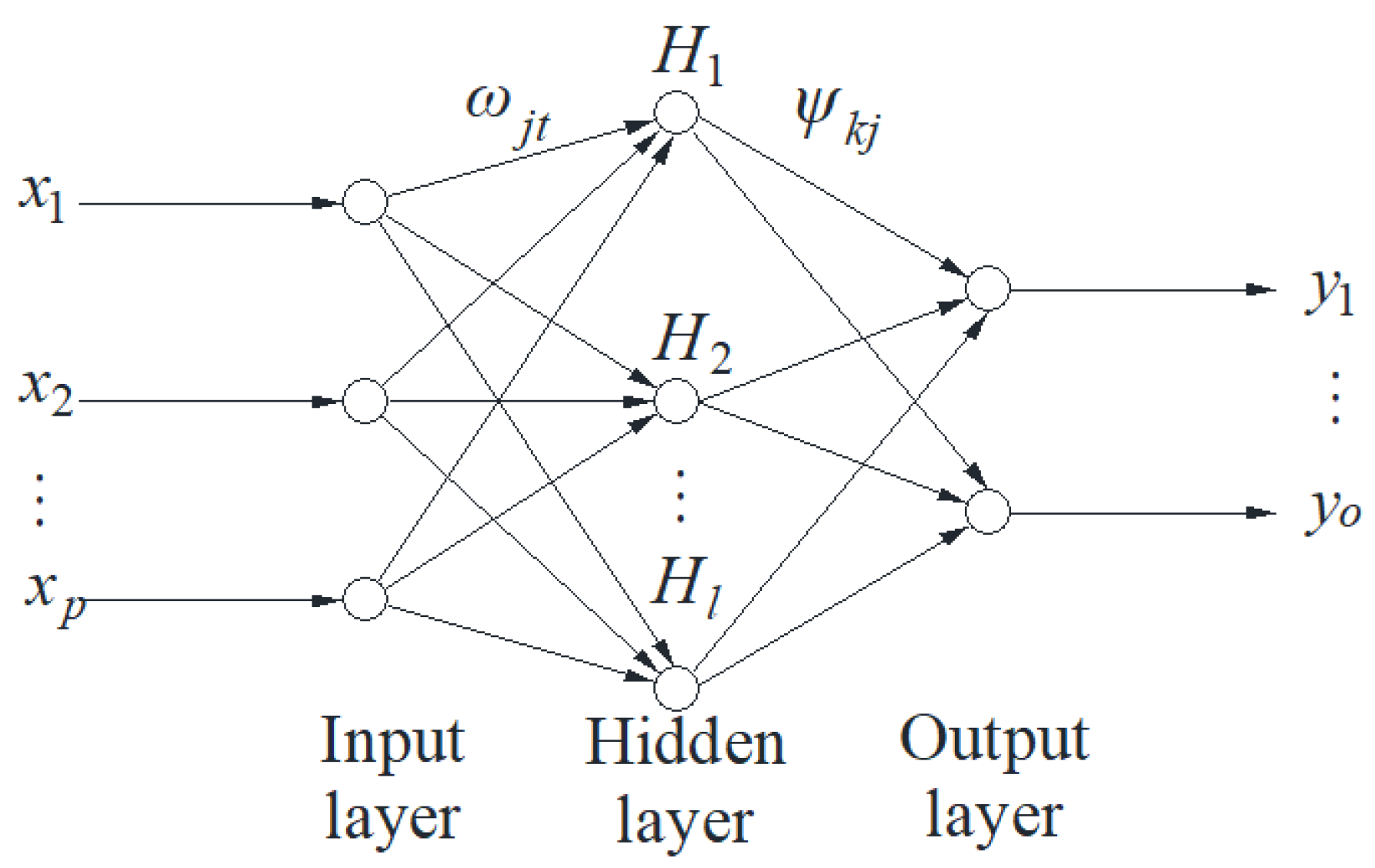
Figure 2.
BPNN learning flowchart.
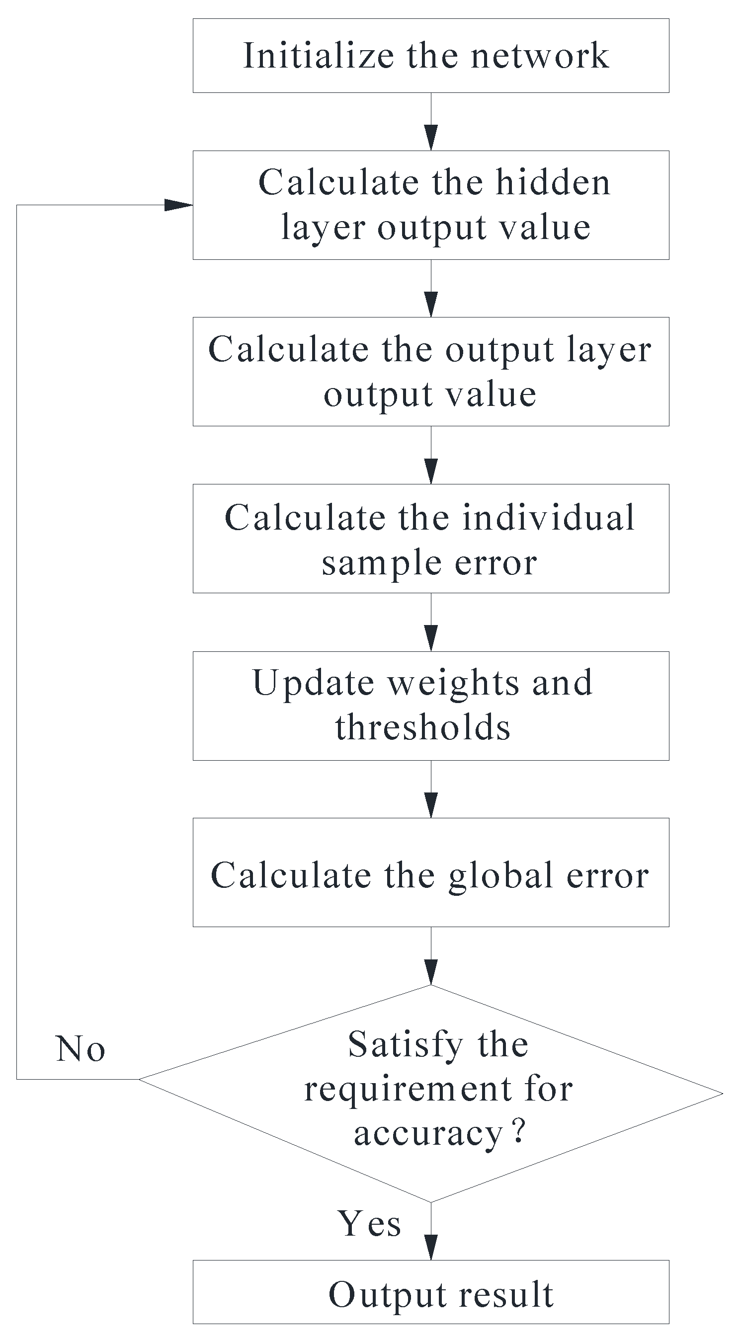
Figure 3.
Learning process of the GABPNN.
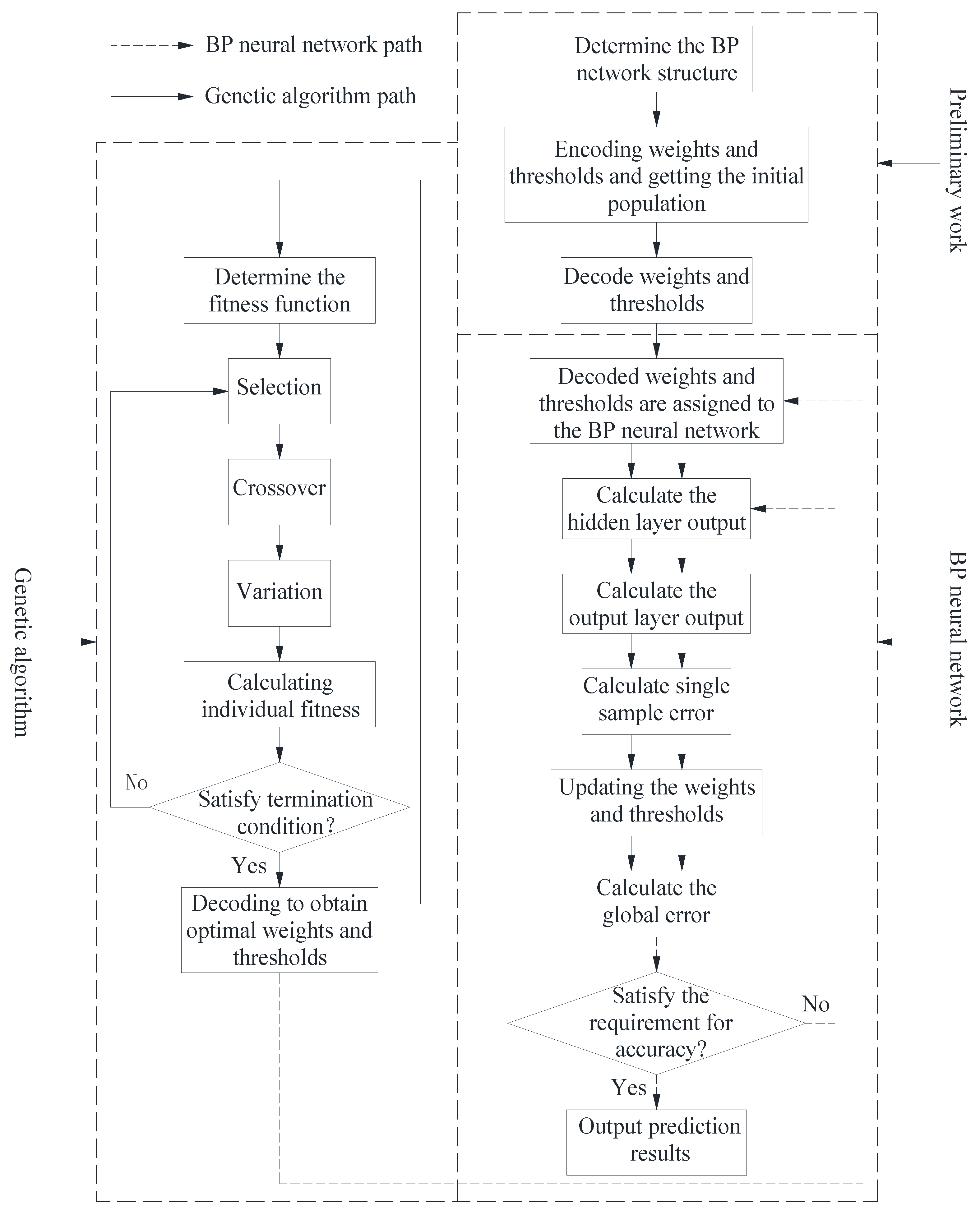
Figure 4.
Structure of the SVR learning machine.
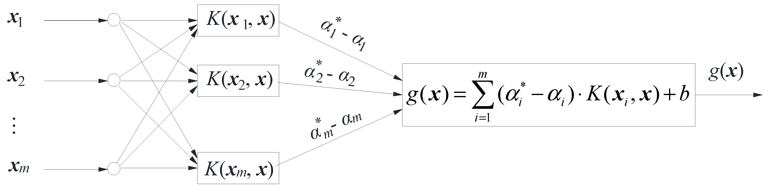
Figure 5.
Flowchart for calculation of comprehensive similarity coefficient.
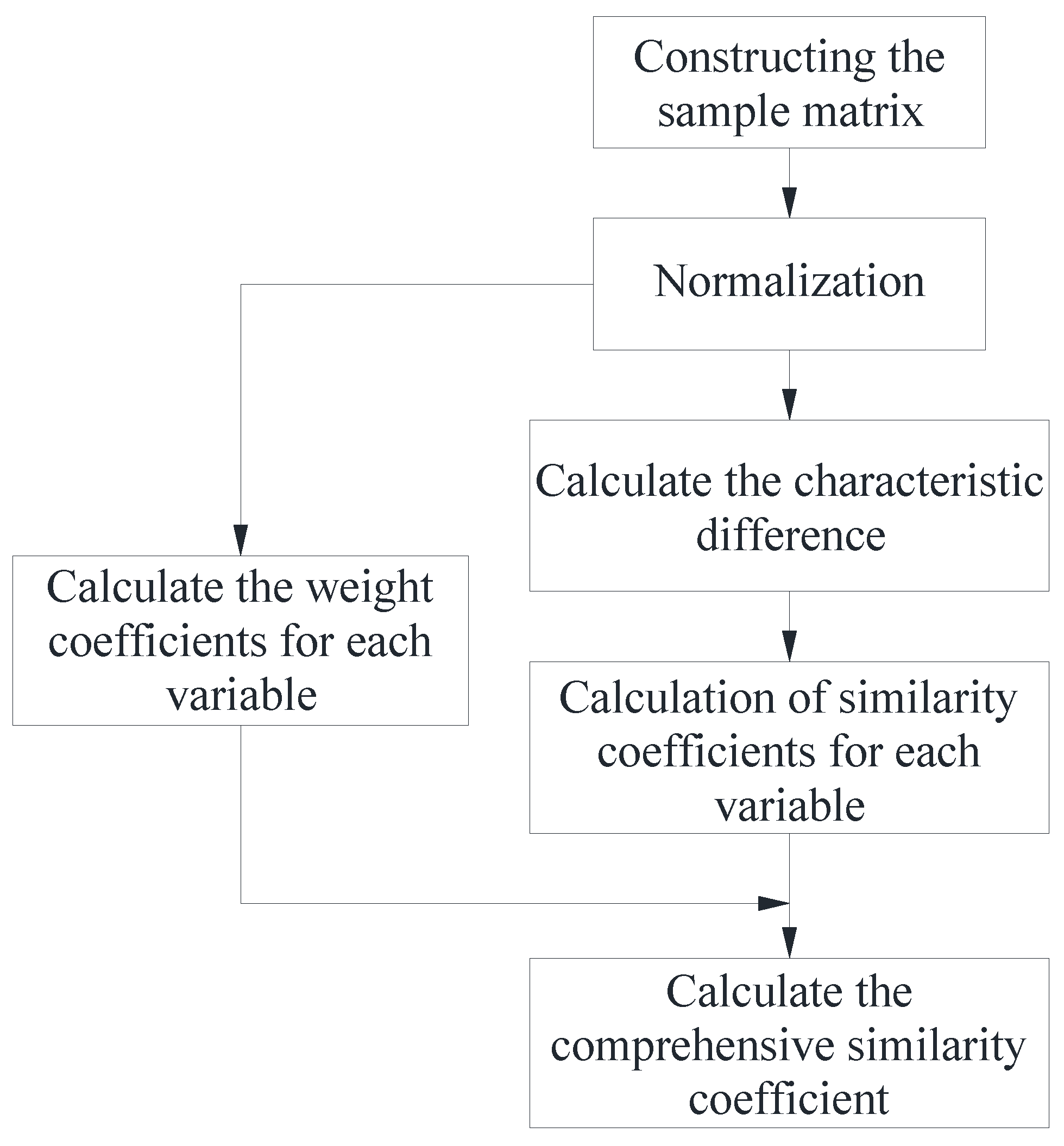
Figure 6.
Prediction flow of artificial intelligence algorithm based on sample similarity improvement.
Figure 6.
Prediction flow of artificial intelligence algorithm based on sample similarity improvement.
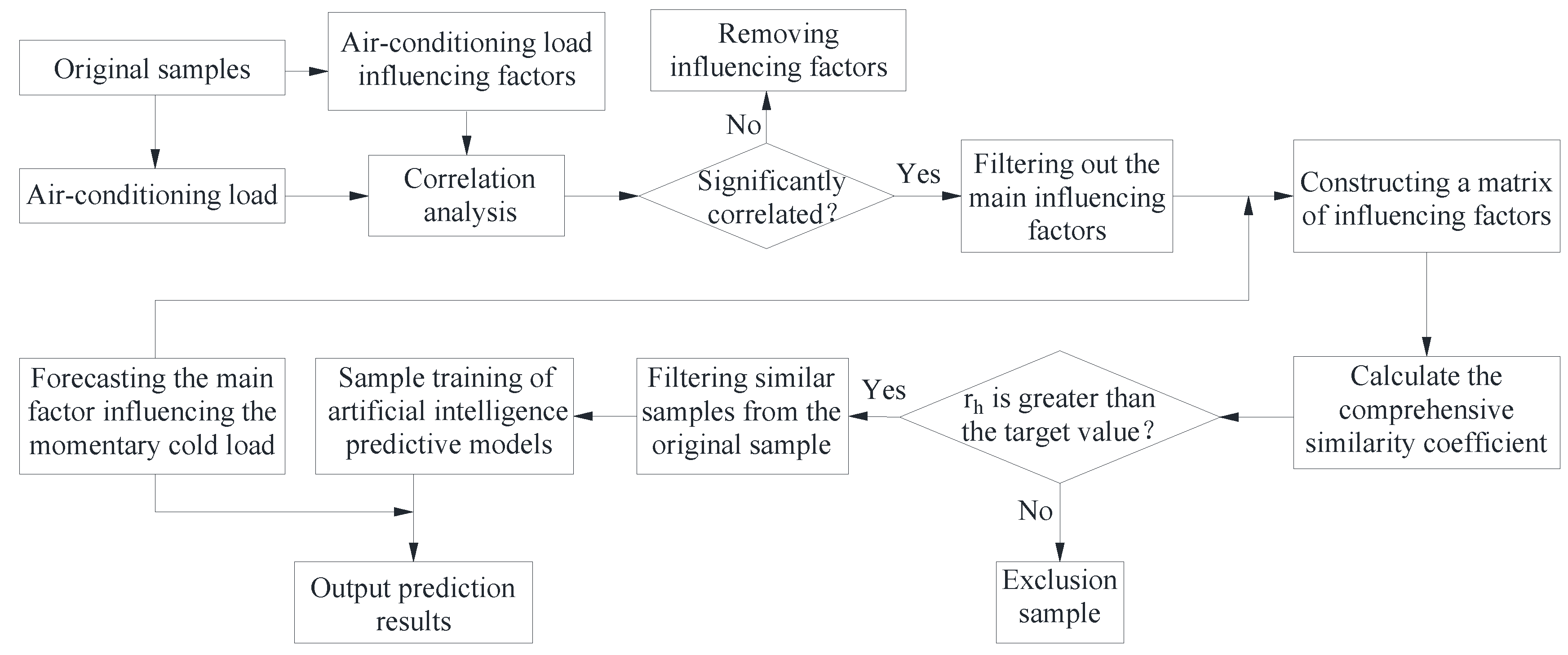
Figure 7.
Variation curves of outdoor temperature and relative humidity.
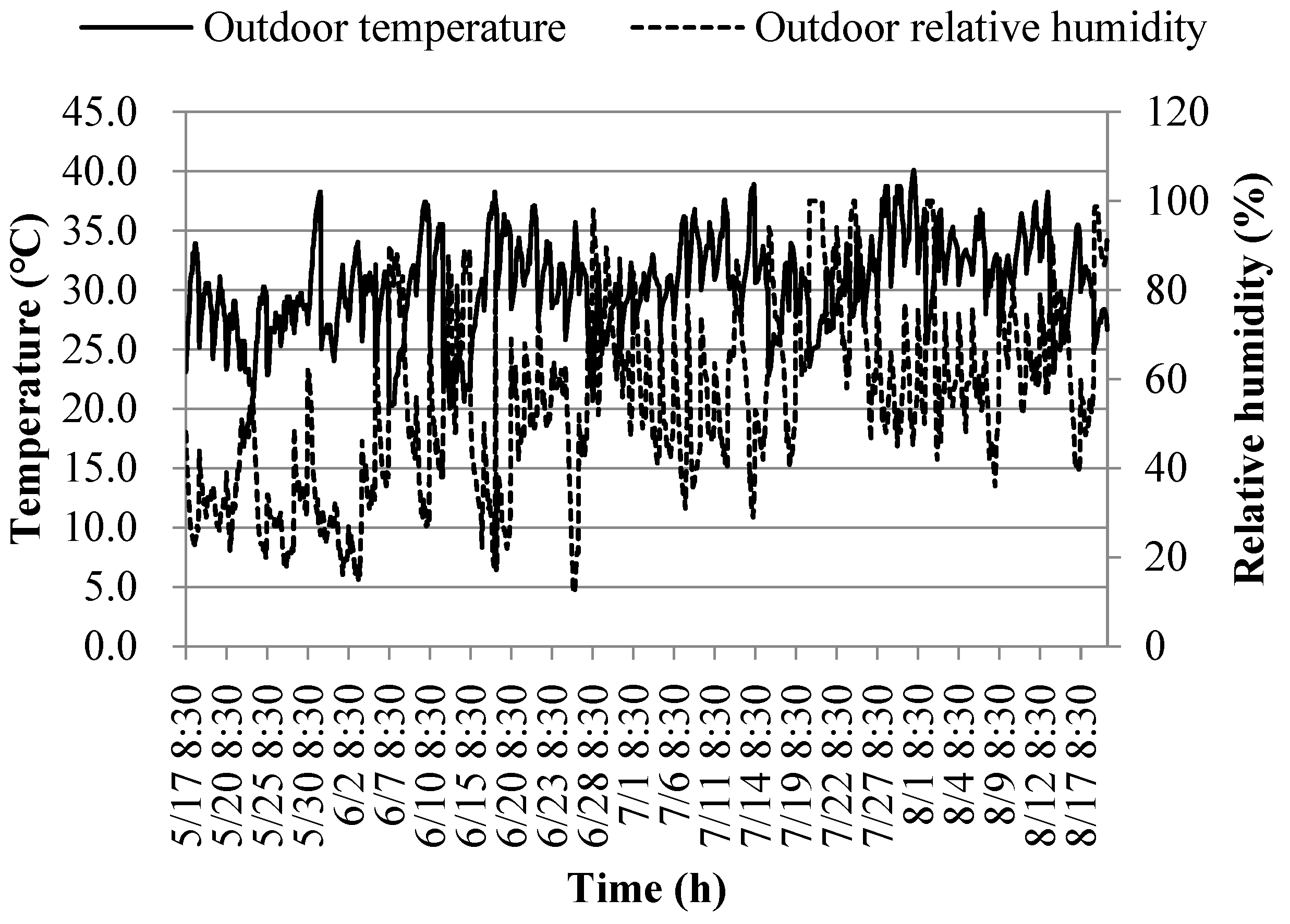
Figure 8.
Variation curves of solar radiation intensity and outdoor wind speed.
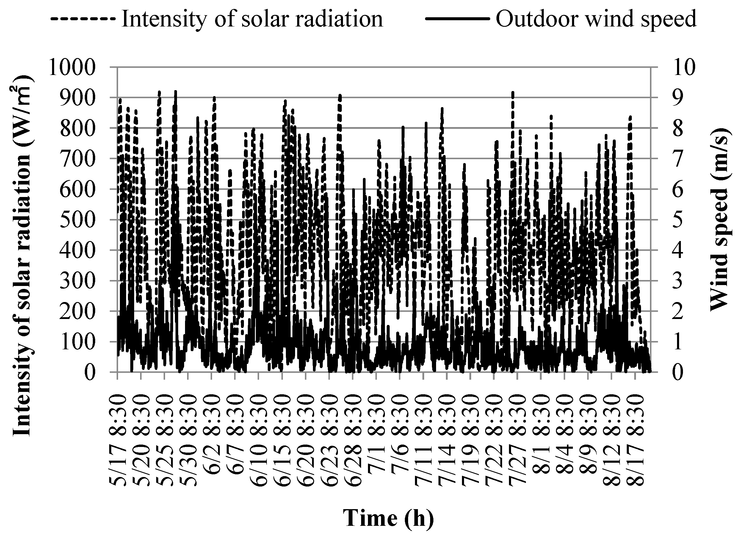
Figure 9.
Measured change curve of cooling capacity of heat pump system.
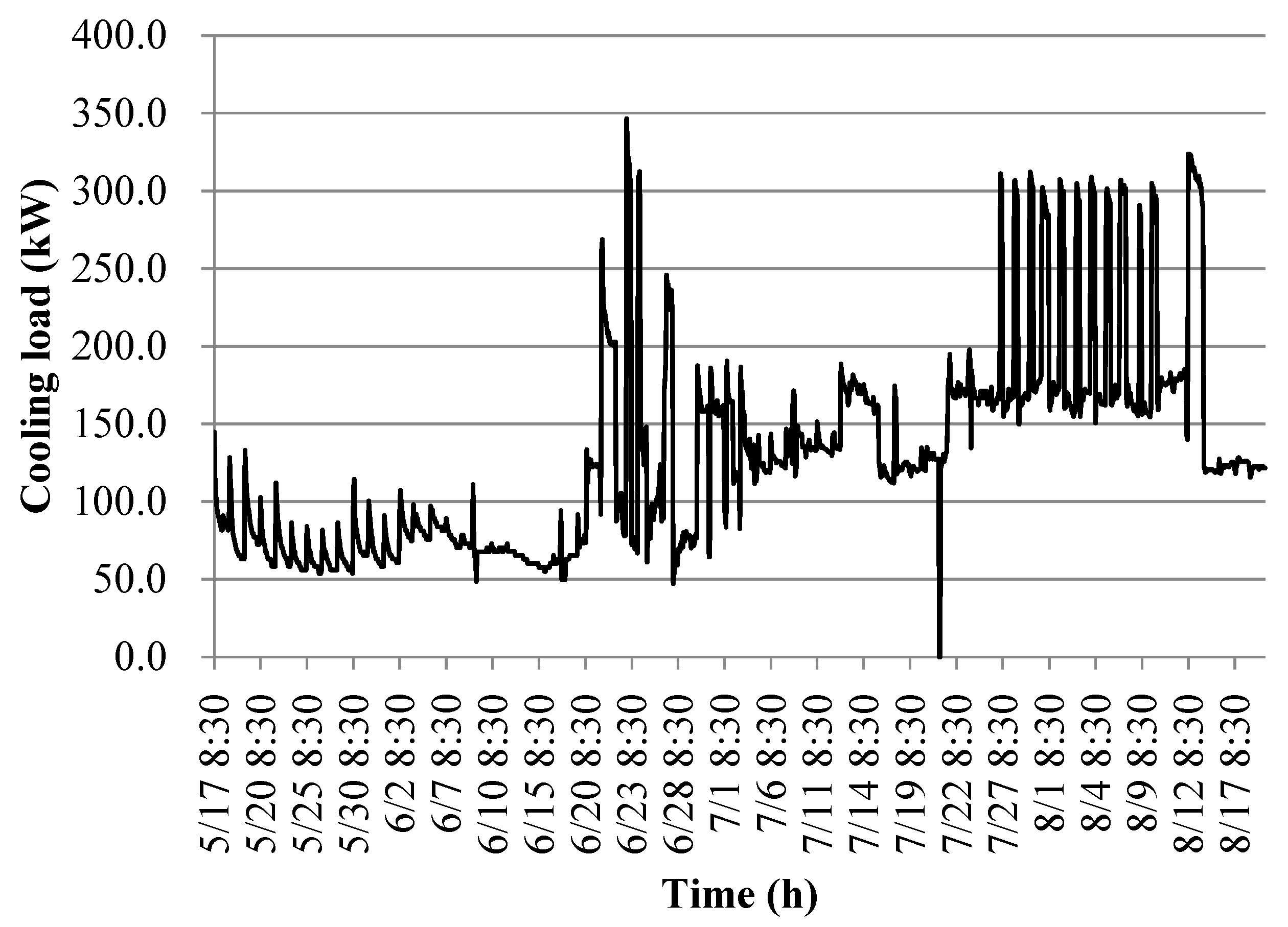
Figure 10.
Distribution of cooling capacity of heat pump system at the early stage of cooling supply.
Figure 10.
Distribution of cooling capacity of heat pump system at the early stage of cooling supply.
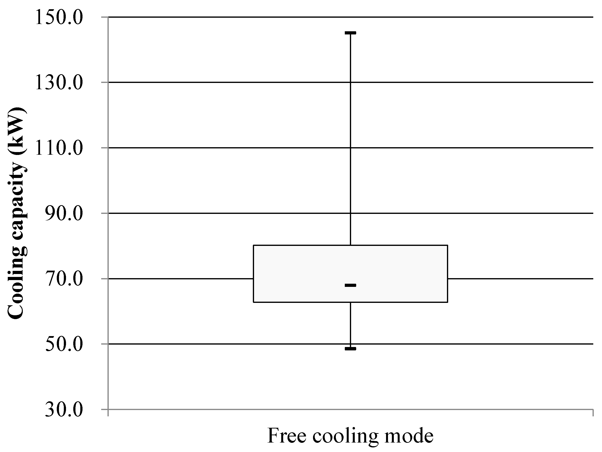
Figure 11.
Distribution of cooling capacity of the heat pump system in the mid-term of the cooling supply.
Figure 11.
Distribution of cooling capacity of the heat pump system in the mid-term of the cooling supply.
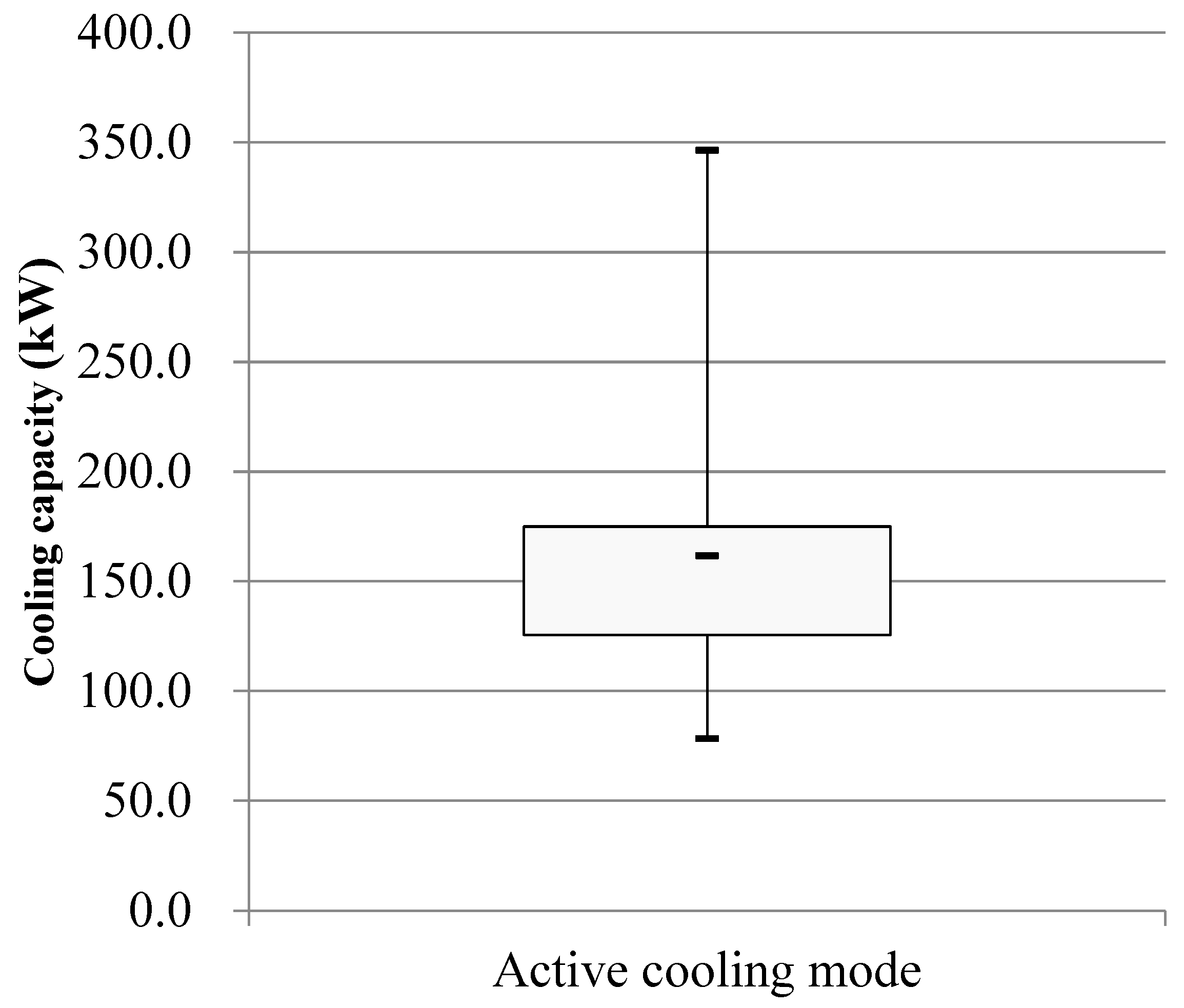
Figure 12.
Variation curves of indoor temperature and relative humidity at the early stage of cooling supply.
Figure 12.
Variation curves of indoor temperature and relative humidity at the early stage of cooling supply.
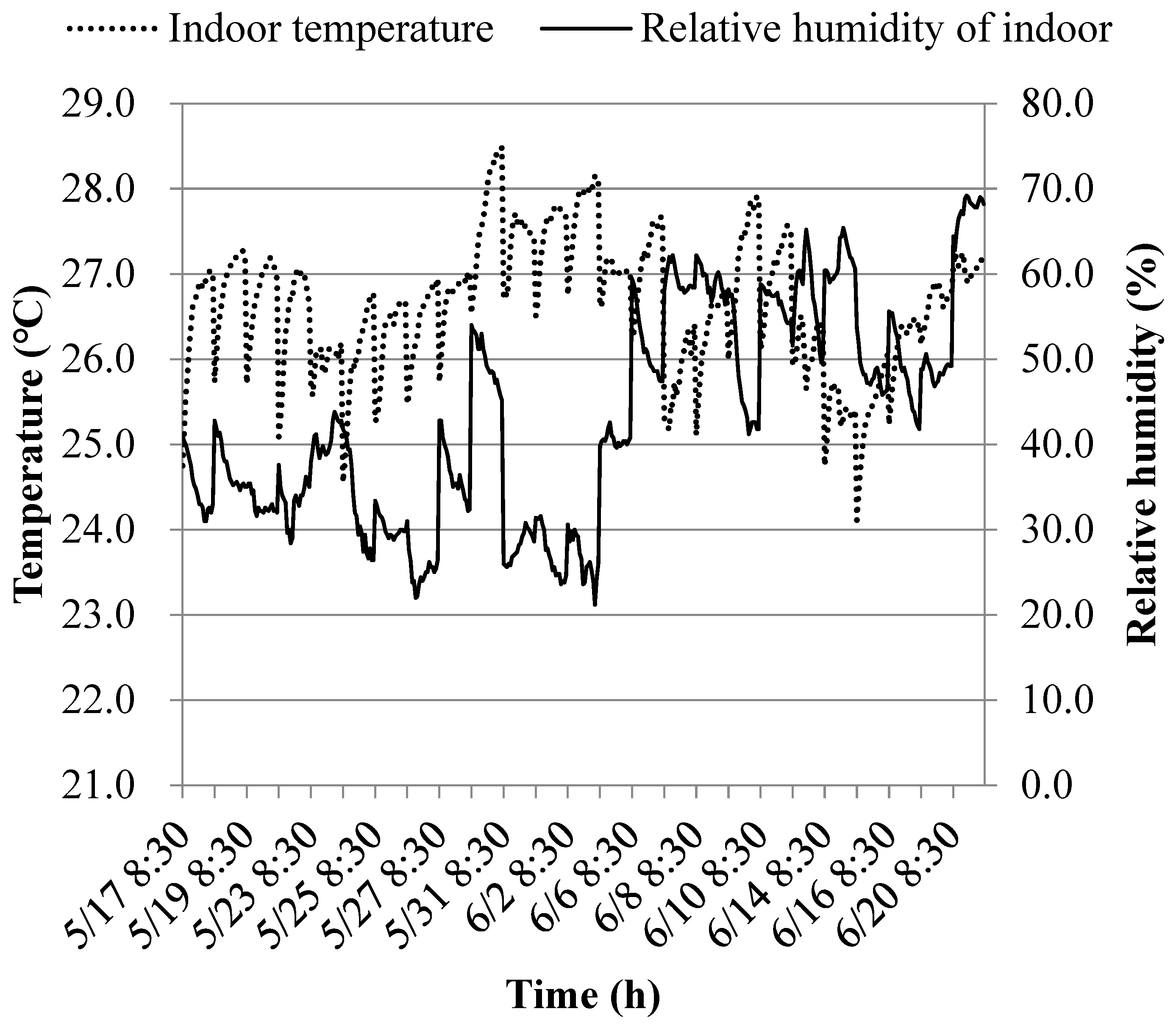
Figure 13.
Variation curves of indoor temperature and relative humidity in the middle stage of cooling supply.
Figure 13.
Variation curves of indoor temperature and relative humidity in the middle stage of cooling supply.
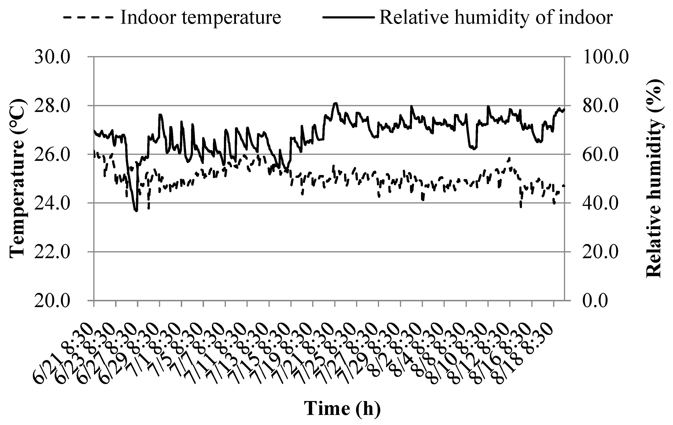
Figure 14.
Comparison of predicted values of model M1 with actual values.
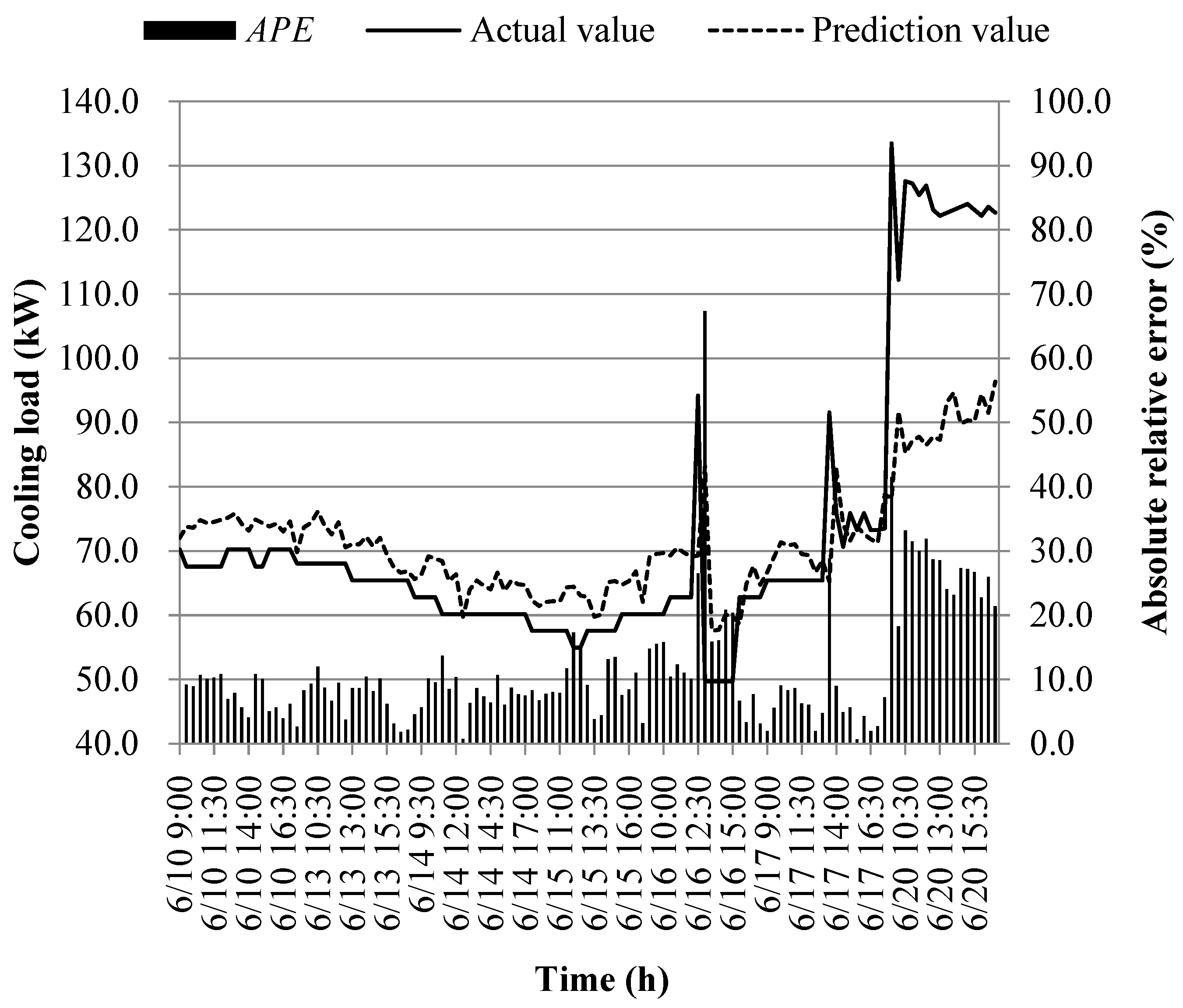
Figure 15.
Comparison of predicted values of model M2 with actual values.
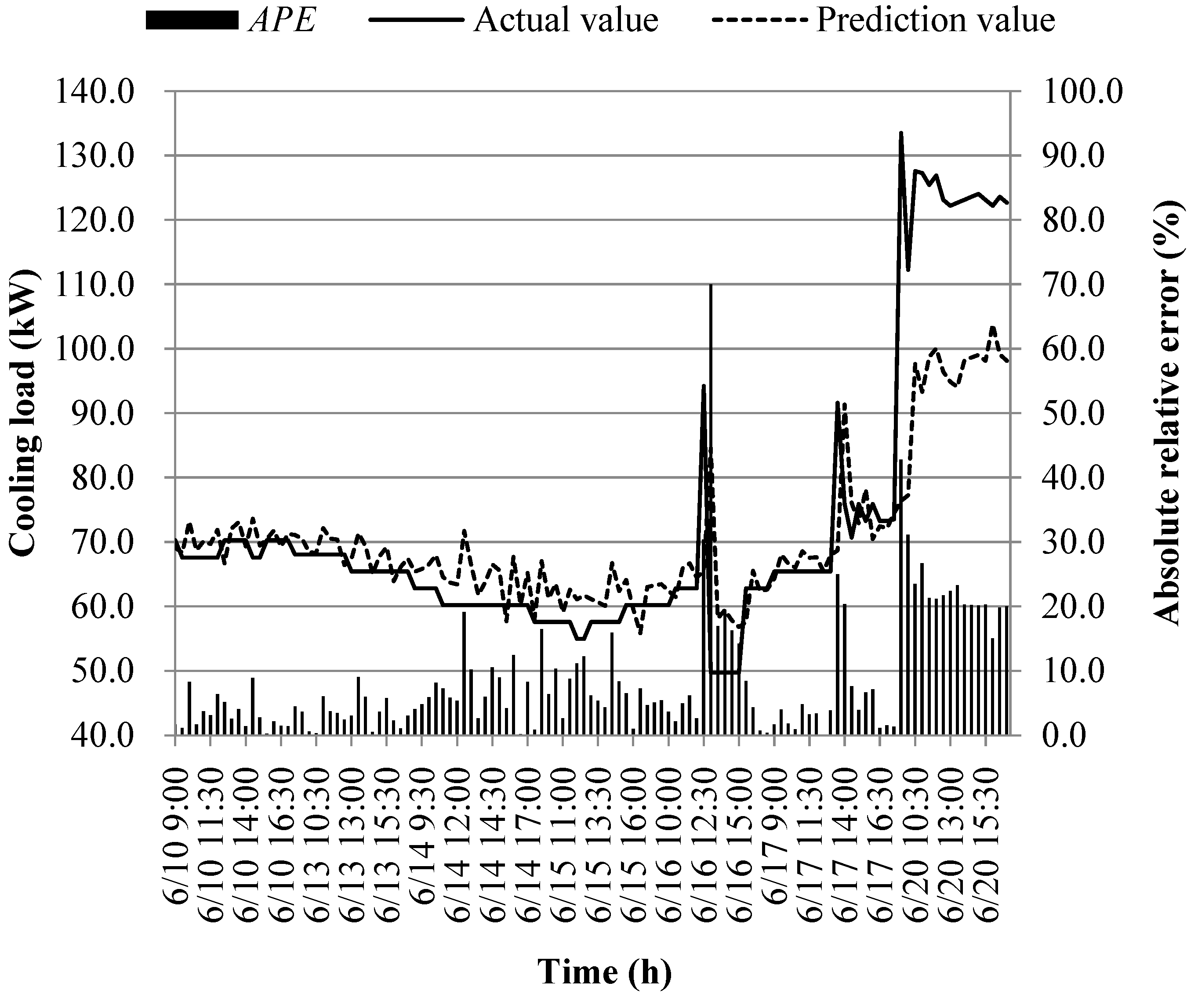
Figure 16.
Comparison of predicted values of model M3 with actual values.
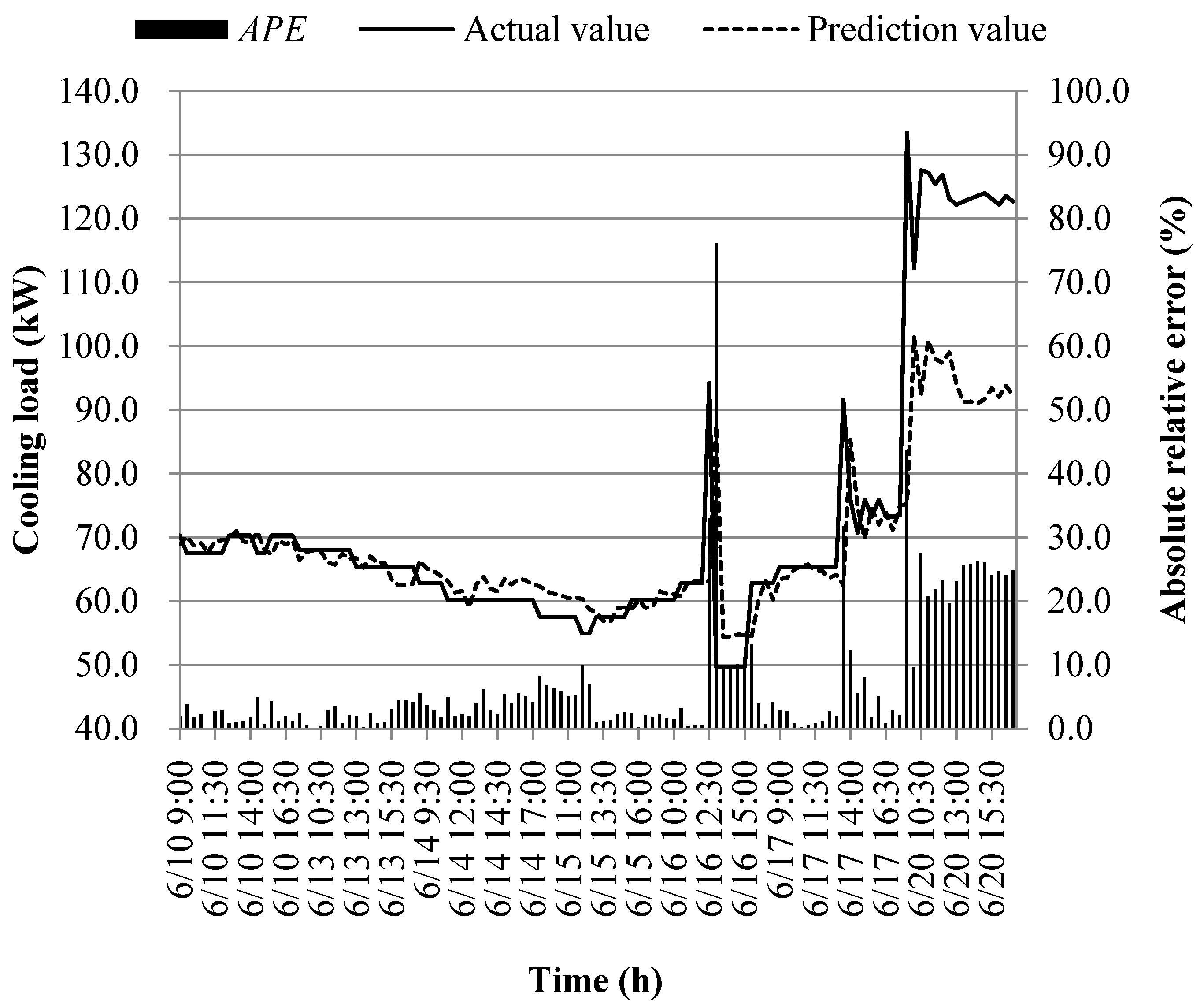
Figure 17.
Comparison of predicted values of model M4 with actual values.
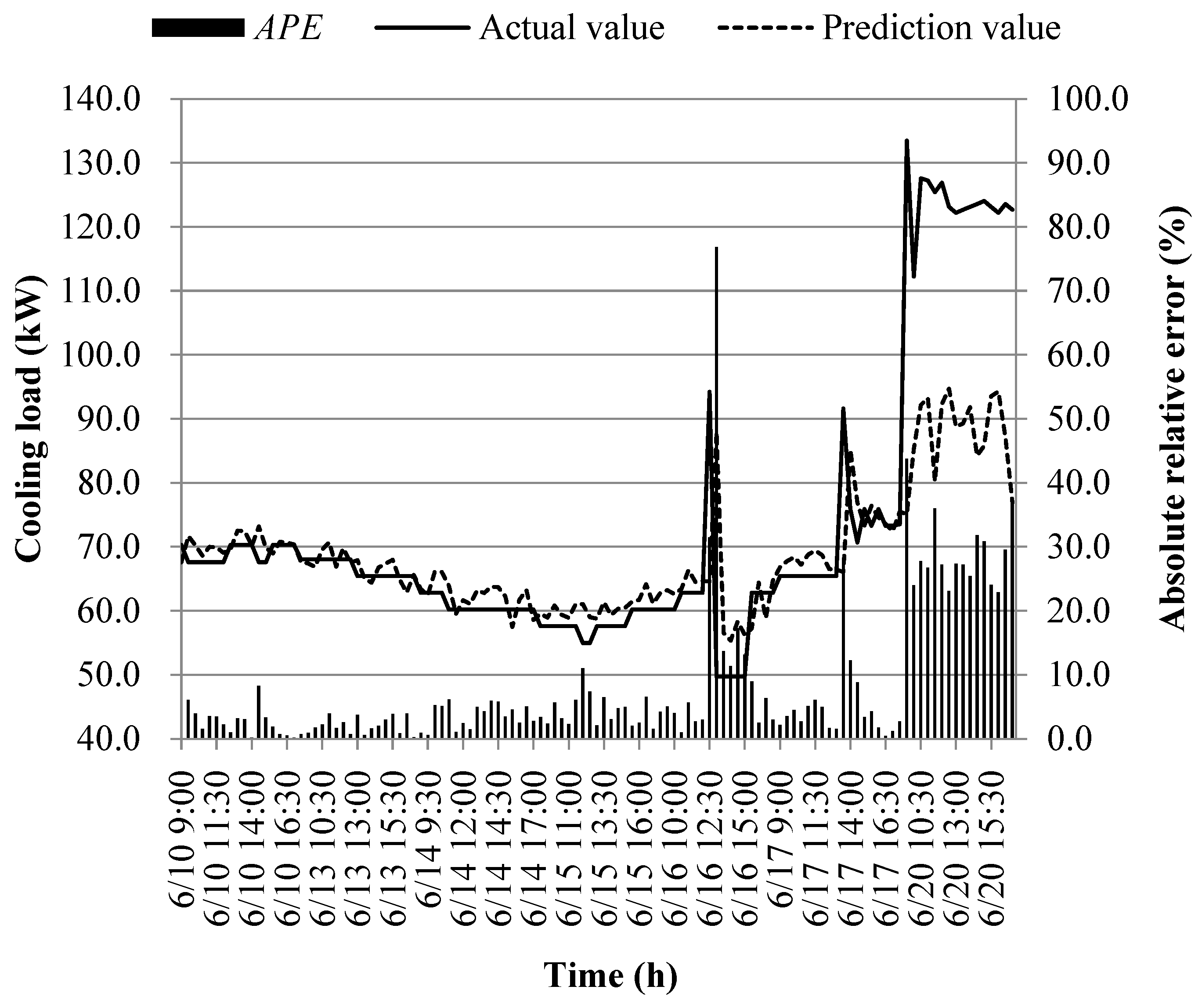
Figure 18.
Comparison of predicted values of model M5 with actual values.
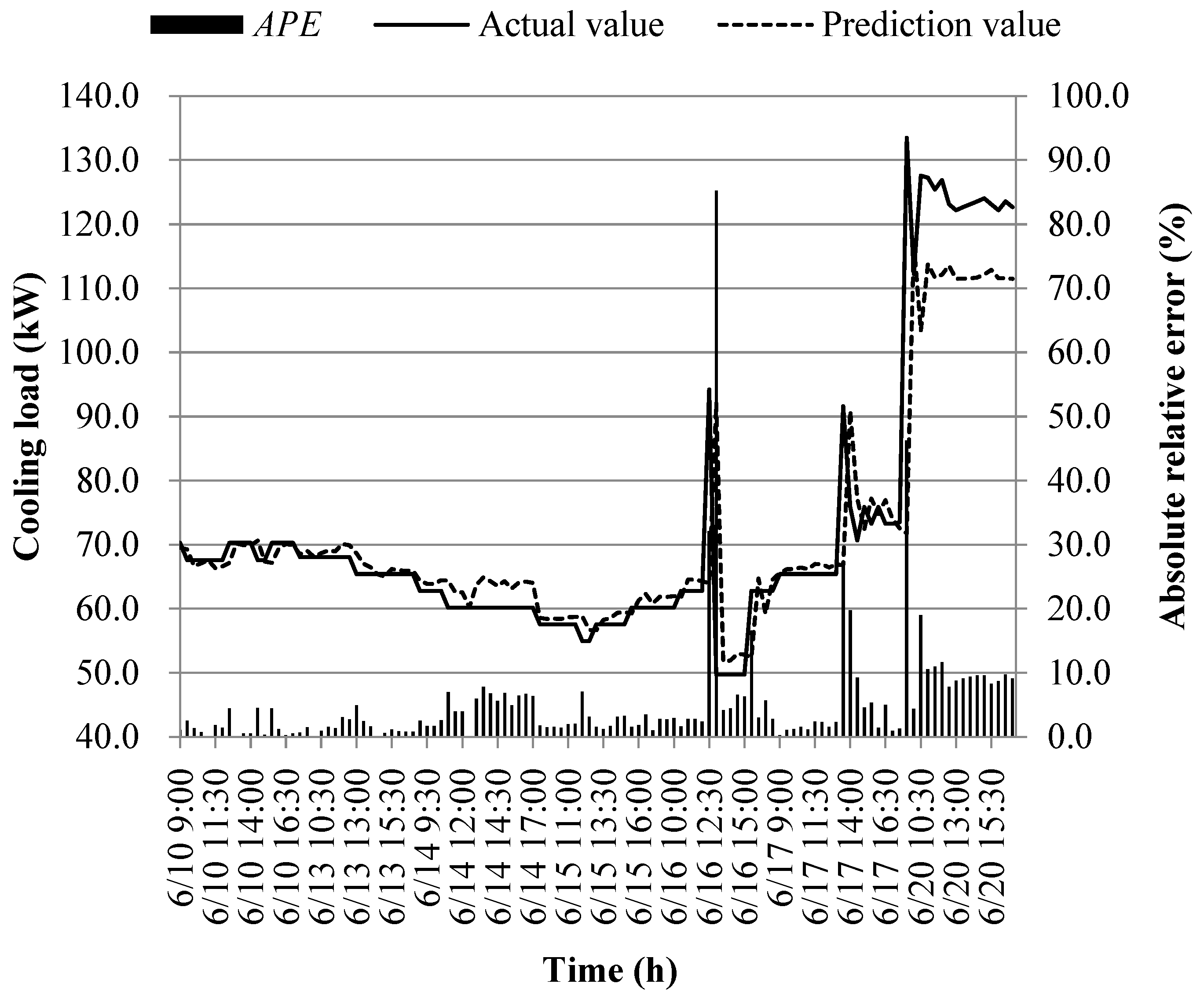
Figure 19.
Comparison of predicted values of model M6 with actual values.
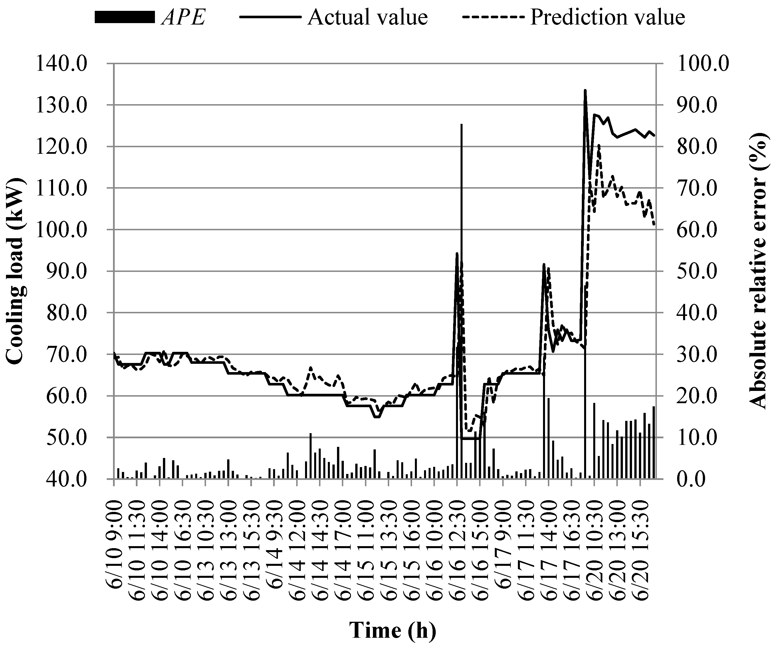
Figure 20.
Comparison of predicted values of model M7 with actual values.
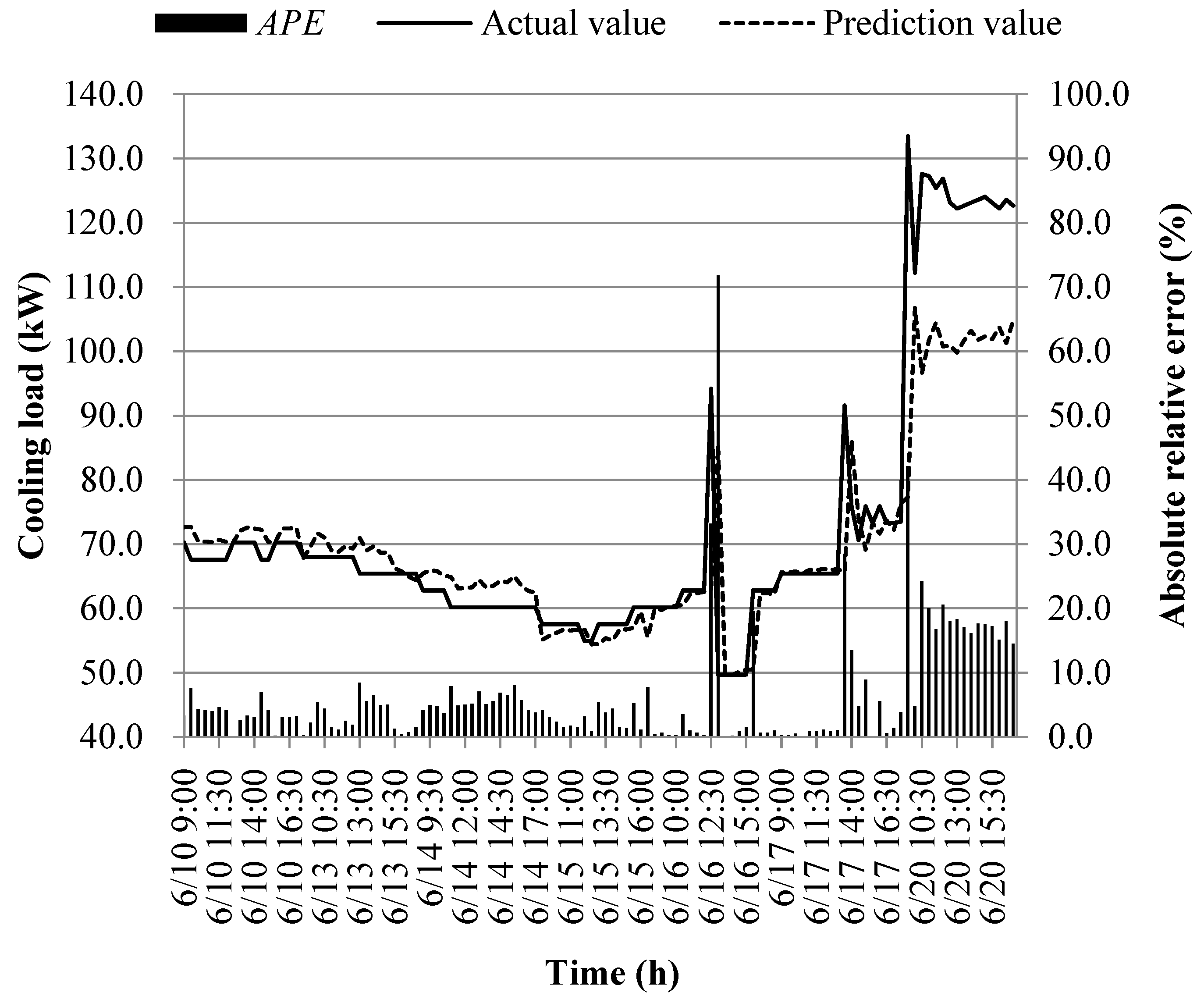
Figure 21.
Comparison of predicted values of model M8 with actual values.
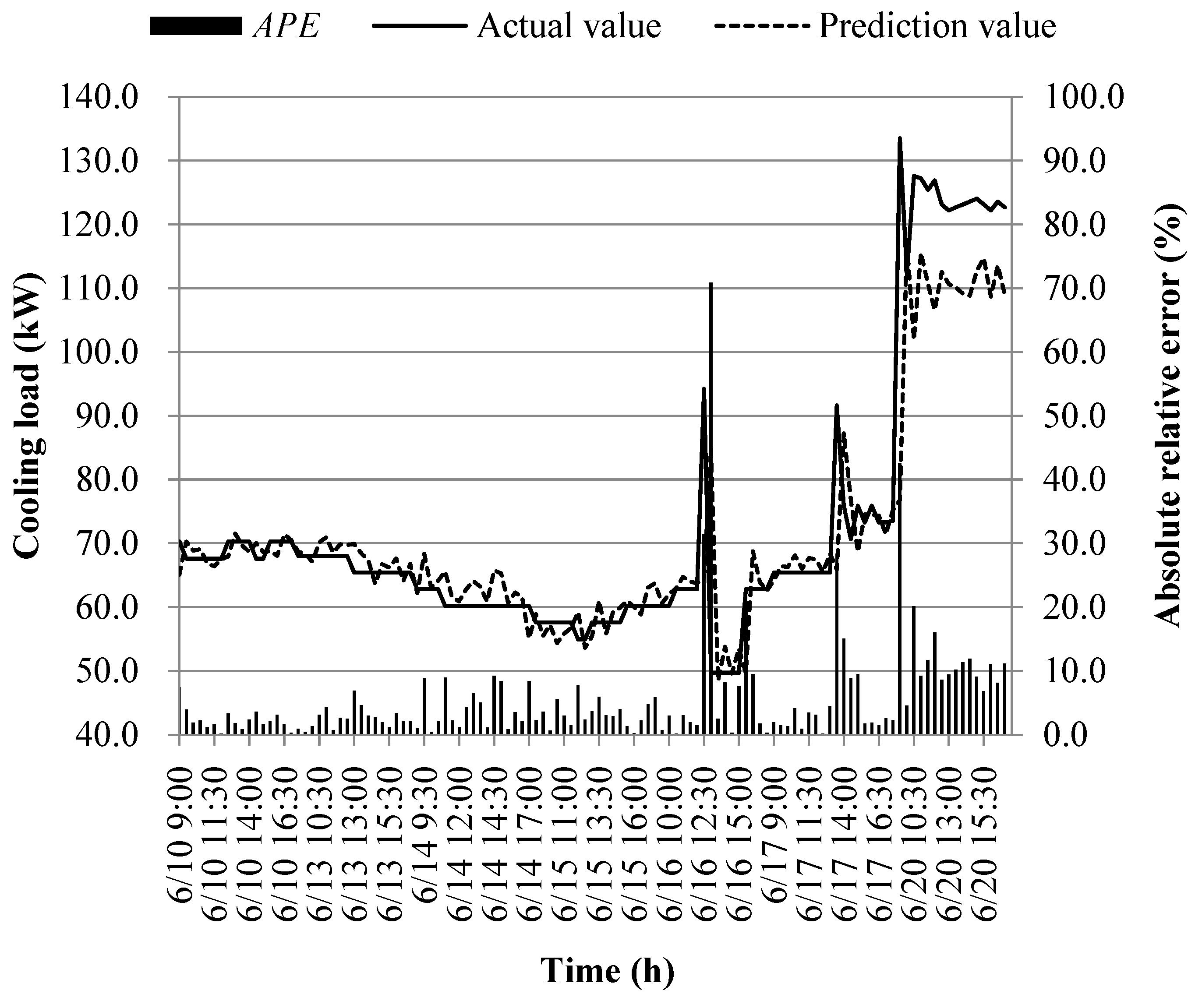
Figure 22.
Distribution interval of absolute relative errors of different prediction models.
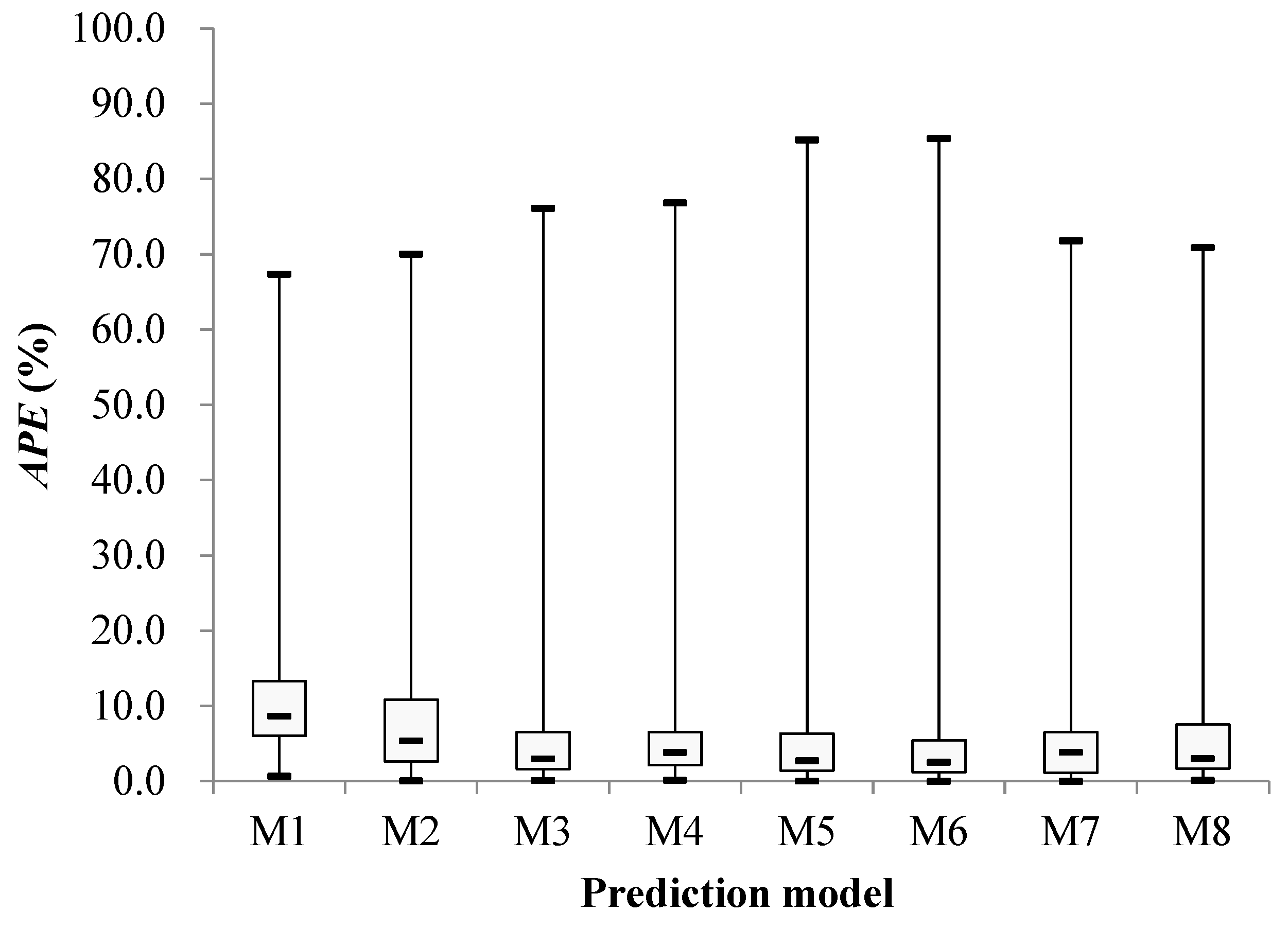
Figure 23.
Comparison of predicted values of model M1 with actual values.
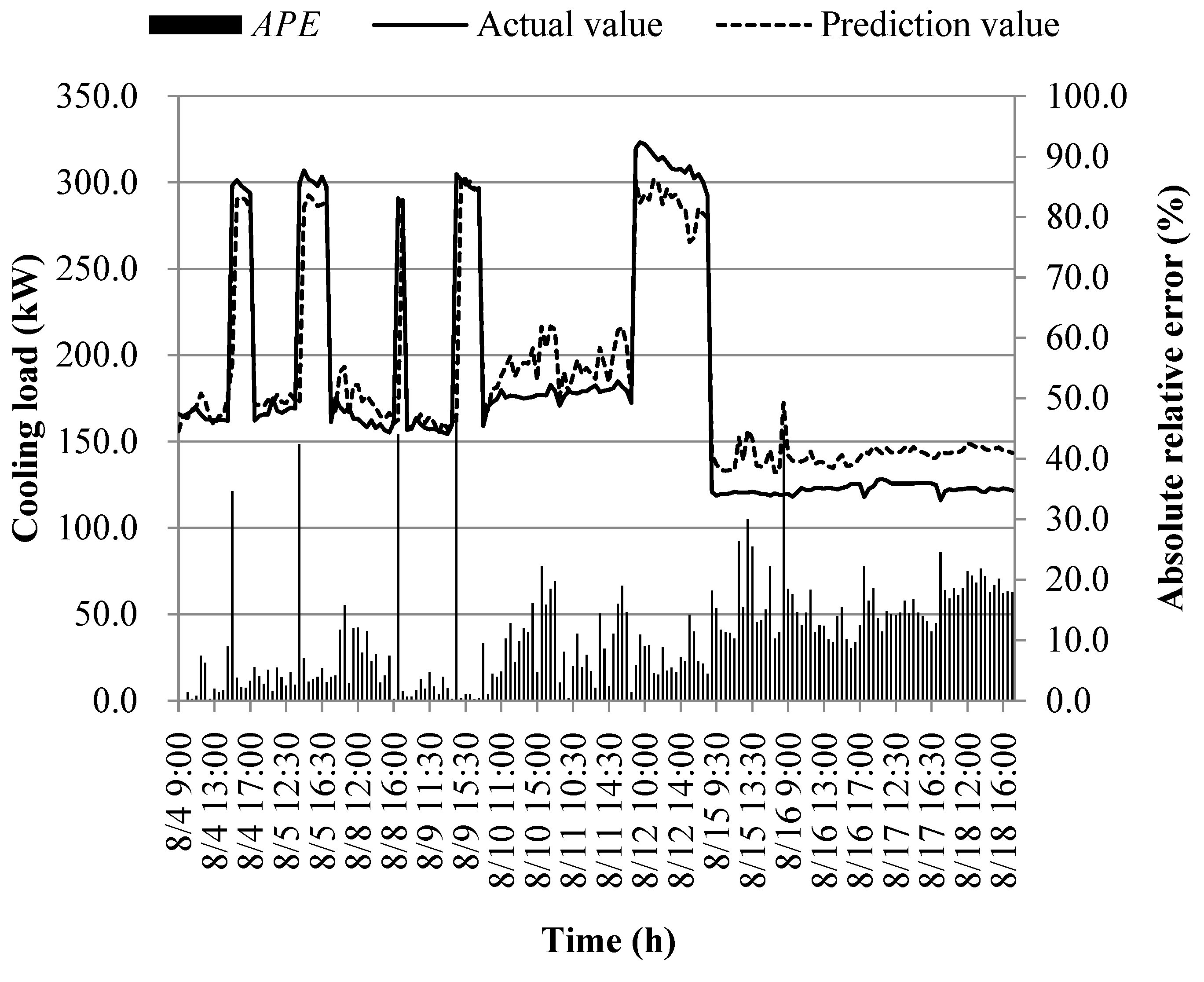
Figure 24.
Comparison of predicted values of model M2 with actual values.
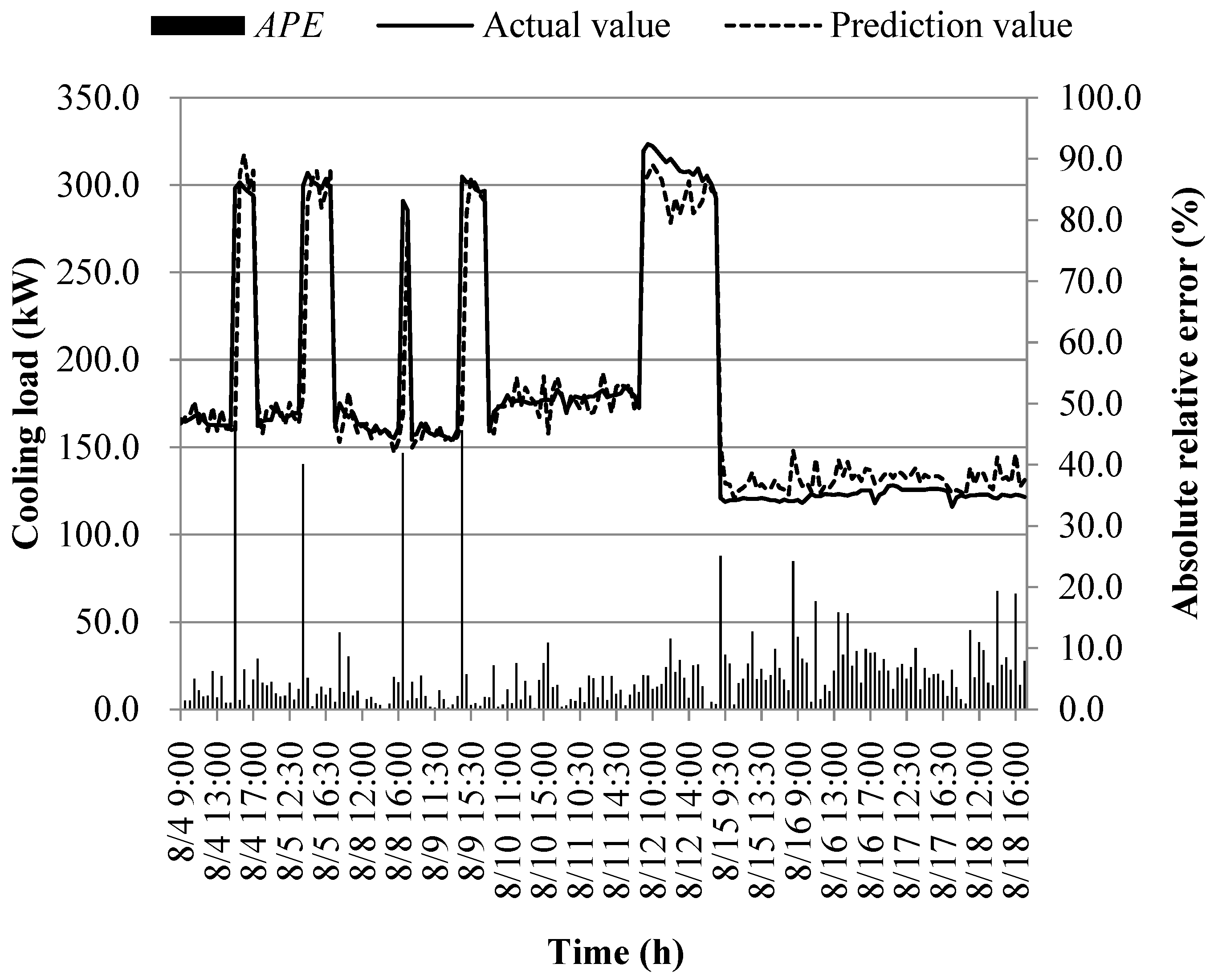
Figure 25.
Comparison of predicted values of model M3 with actual values.
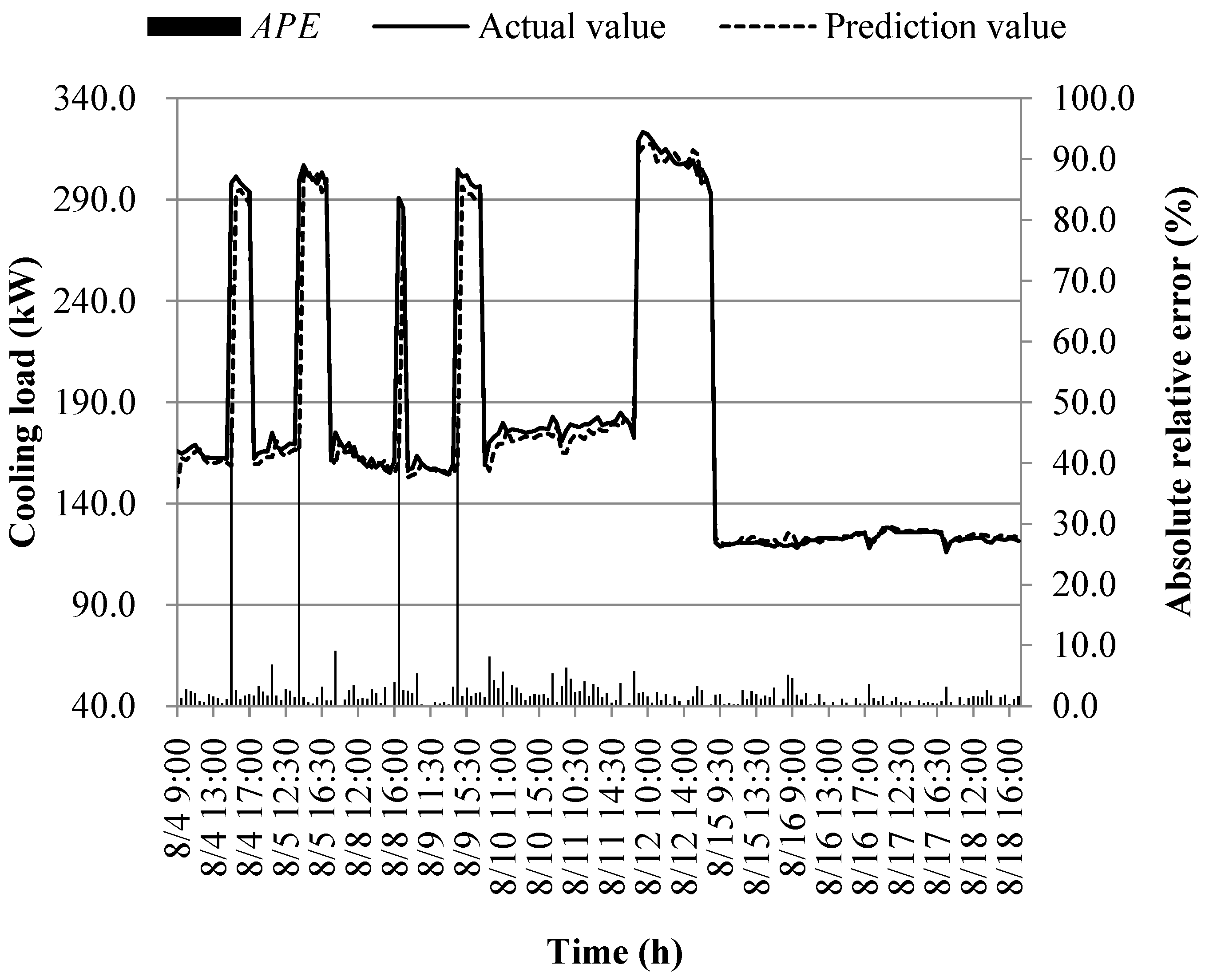
Figure 26.
Comparison of predicted values of model M4 with actual values.
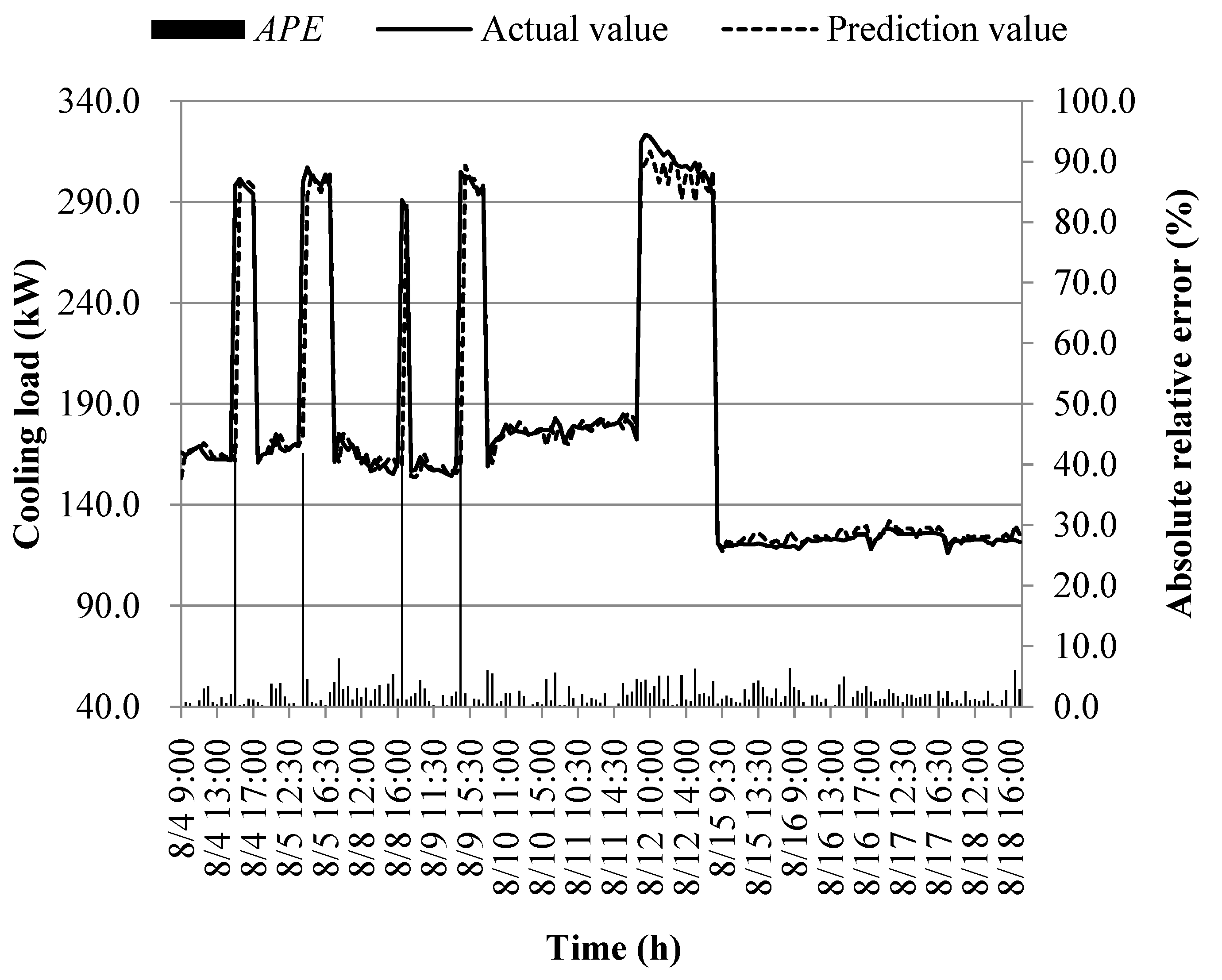
Figure 27.
Comparison of predicted values of model M5 with actual values.

Figure 28.
Comparison of predicted values of model M6 with actual values.
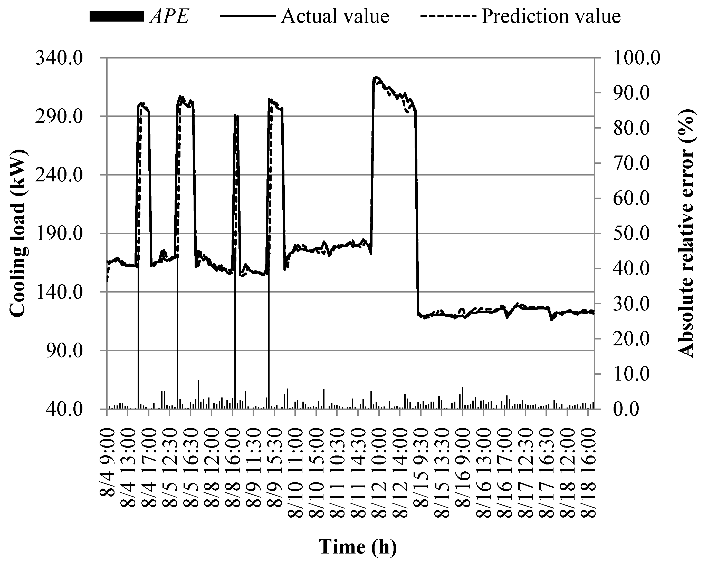
Figure 29.
Comparison of predicted values of model M7 with actual values.

Figure 30.
Comparison of predicted values of model M8 with actual values.
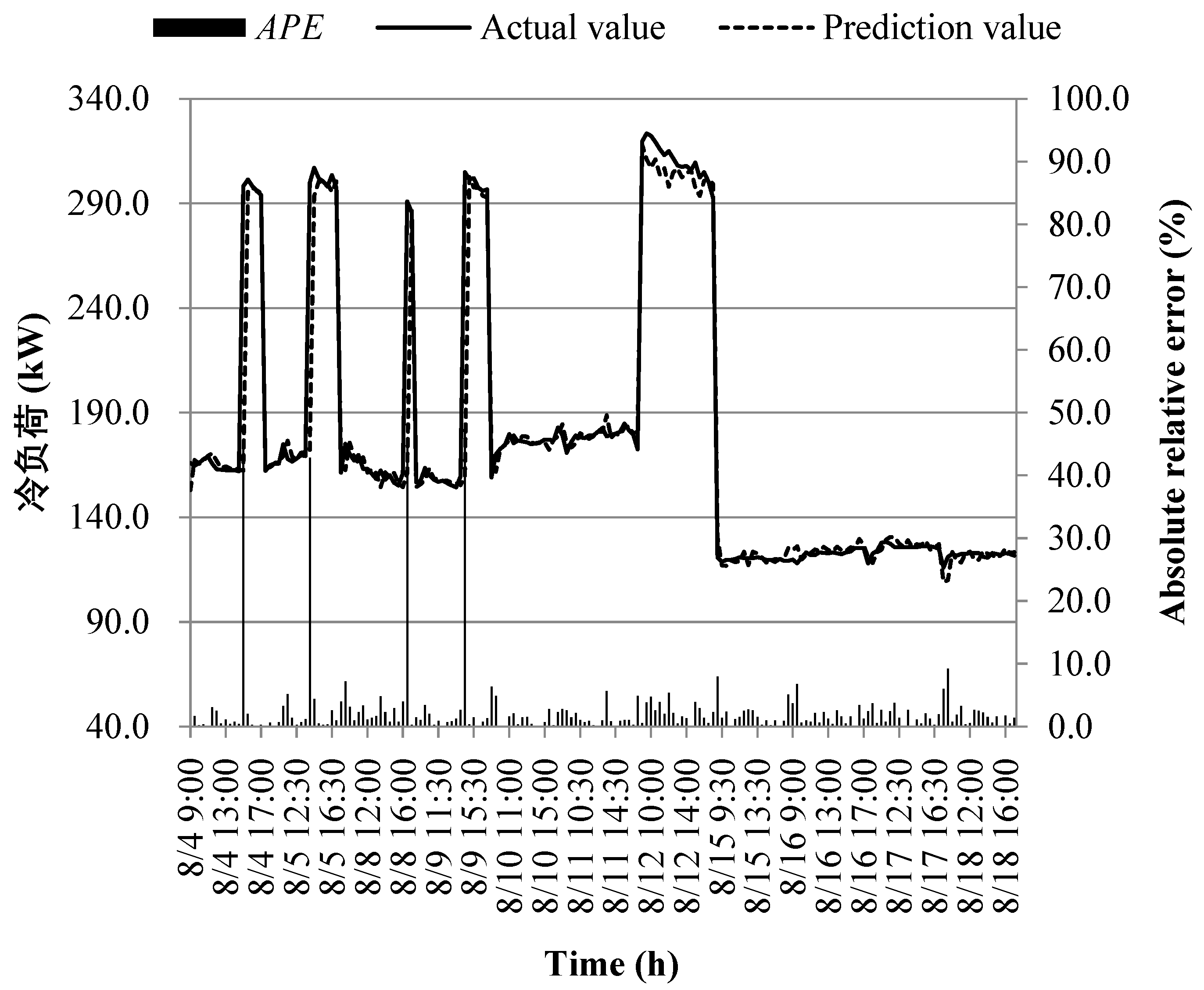
Figure 31.
Distribution interval of absolute relative errors of different prediction models.
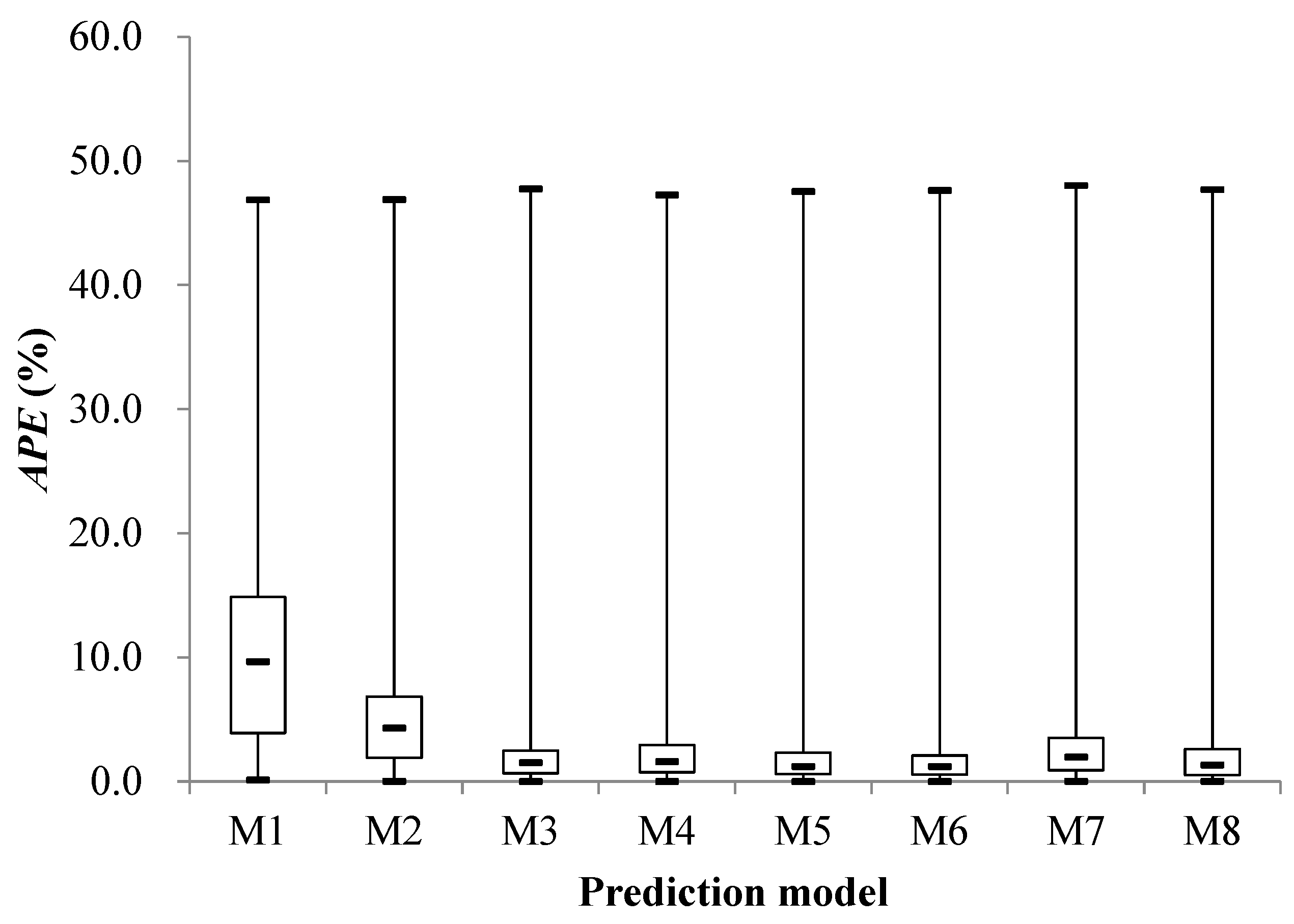

Table 1.
Detailed parameters of the test instrument (component).
| Instrument name. | Model | Test range | Precision |
|---|---|---|---|
| heat meter | Engelmann SENSOSTAR 2BU | Temperature: 1~150℃/Flow rate: 0~120m³/h | ±0.35℃/±2% |
| HOBO data self-logger | U10-003 | Temperature: -20~70℃ / Relative humidity: 25~95% | ±0.4℃/±3.5% |
| Temperature and HumiditySensor (small weather station) | S-THB-M002 | Temperature: -40~75℃/Relative Humidity:0~100% | ±0.21℃/±2.5% |
| Solar Radiation Sensor(small meteorological station) | S-LIB-M003 | 0~1280W/m2 | ±10W/m2 |
| Wind Speed Sensor(small meteorological station) | S-WSB-M003 | 0~76m/s | ±4% |
Table 2.
Testing and the relative uncertainty of calculated parameters.
| Parameter name | Unit | Relative uncertainty (%) |
|---|---|---|
| Return water temperature of free cooling mode | ℃ | ±1.06 |
| Supply water temperature of free cooling mode | ℃ | ±1.25 |
| Cooling capacity of free cooling model | kW | ±9.77 |
| Flow of free cooling model | m3/h | ±1.77 |
| Indoor temperature | ℃ | ±0.90 |
| Relative humidity of indoor air | % | ±3.26 |
| outdoor temperature | ℃ | ±0.40 |
| Relative humidity of outdoor | % | ±2.65 |
| Intensity of solar radiation | W/m2 | ±1.49 |
| Outdoor wind speed | m/s | ±2.31 |
| Water supply temperature of heat pump unit A | ℃ | ±2.43 |
| Return water temperature of heat pump unit A | ℃ | ±1.67 |
| Cooling capacity of heat pump unit A | kW | ±7.56 |
| Cooling energy efficiency of heat pump unit A | - | ±7.53 |
| Water supply temperature of heat pump unit B | ℃ | ±1.88 |
| Return water temperature of heat pump unit B | ℃ | ±1.44 |
| Cooling capacity of heat pump unit B | kW | ±8.69 |
Table 3.
Main parameter settings of the genetic algorithm.
| Number of populations | 50 |
|---|---|
| Maximum number of generations | 400 |
| The number of binary digits of the variable | 20 |
| Generation gap | 0.95 |
| Probability of crossover | 0.7 |
| Probability of mutation | 0.01 |
Table 4.
Main parameter settings of BPNN.
| Maximum training times | 1000 |
|---|---|
| Momentum factor | 0.9 |
| Learning rate | 0.1 |
| Training goal | 0.005 |
Table 5.
Normal distribution test of factors influencing building cooling load in the early stage of cooling supply.
Table 5.
Normal distribution test of factors influencing building cooling load in the early stage of cooling supply.
| Indicators | Building cooling load and its influencing factors | |||||||
|---|---|---|---|---|---|---|---|---|
| Q | To | RHo | Io | Vo | Ti | RHi | Q(t-1) | |
| Average value |
72.766 | 29.013 | 39.697 | 476.889 | 1.060 | 26.675 | 43.249 | 73.980 |
| Standard deviation |
15.523 | 4.123 | 18.196 | 238.526 | 0.871 | 0.755 | 12.712 | 16.471 |
| Test statistic |
0.147 | 0.041 | 0.156 | 0.061 | 0.124 | 0.051 | 0.098 | 0.146 |
| Asymptotic significance |
0.000 | 0.089 | 0.000 | 0.001 | 0.000 | 0.011 | 0.000 | 0.000 |
Note: Q(t-1) represents the sequence of cooling loads at the previous moment (time interval of 0.5h).
Table 6.
Results of correlation analysis between building cooling load and its influencing factors in the early stage of cooling supply.
Table 6.
Results of correlation analysis between building cooling load and its influencing factors in the early stage of cooling supply.
| Indicator | Factors affecting building cooling loads | ||||||
|---|---|---|---|---|---|---|---|
| To | RHo | Io | Vo | Ti | RHi | Q(t-1) | |
| Correlation coefficient | 0.119* | 0.171** | 0.144** | -0.129** | 0.221** | 0.180** | 0.956** |
| Significance | 0.014 | 0.000 | 0.003 | 0.008 | 0.000 | 0.000 | 0.000 |
Note: ** is used to indicate that two variables are significantly correlated at the 0.01 level.
Table 7.
Detailed information on different prediction models for the early stage of cooling supply.
| Name | Main Input Variables | Detailed description |
|---|---|---|
| M1 | HRo; Io; Vo; Ti; RHi; Q(t-1) | BPNN |
| M2 | HRo; Io; Vo; Ti; RHi; Q(t-1) | Similar samples screening +BPNN |
| M3 | HRo; Io; Vo; Ti; RHi; Q(t-1) | GABPNN |
| M4 | HRo; Io; Vo; Ti; RHi; Q(t-1) | Similar samples screening +GABPNN |
| M5 | HRo; Io; Vo; Ti; RHi; Q(t-1) | SVR neural network |
| M6 | HRo; Io; Vo; Ti; RHi; Q(t-1) | Similar samples screening +SVR neural network |
| M7 | HRo; Io; Vo; Ti; RHi; Q(t-1) | ELM neural network |
| M8 | HRo; Io; Vo; Ti; RHi; Q(t-1) | Similar samples screening +ELM neural network |
Table 8.
Evaluation of the prediction effect of different prediction models.
| Model | Training error | Prediction error | ||||
|---|---|---|---|---|---|---|
| MAPE(%) | R2 | RMSE(kW) | MAPE(%) | R2 | RMSE(kW) | |
| M1 | 3.7 | 0.892 | 4.092 | 11.5 | 0.535 | 14.611 |
| M2 | 3.5 | 0.895 | 3.937 | 8.8 | 0.658 | 12.536 |
| M3 | 2.6 | 0.917 | 3.593 | 7.2 | 0.632 | 12.992 |
| M4 | 2.9 | 0.915 | 3.531 | 8.3 | 0.528 | 14.717 |
| M5 | 2.2 | 0.908 | 3.777 | 5.4 | 0.811 | 9.319 |
| M6 | 2.5 | 0.903 | 3.763 | 5.7 | 0.782 | 10.007 |
| M7 | 2.8 | 0.903 | 3.889 | 6.4 | 0.742 | 10.881 |
| M8 | 3.0 | 0.897 | 3.885 | 5.7 | 0.820 | 9.101 |
Table 9.
Normal distribution test of factors influencing building cooling load in the middle stage of cooling supply.
Table 9.
Normal distribution test of factors influencing building cooling load in the middle stage of cooling supply.
| Indicators | Building cooling load and its influencing factors | |||||||
|---|---|---|---|---|---|---|---|---|
| Q | To | RHo | Io | Vo | Ti | RHi | Q(t-1) | |
| Average value |
169.105 | 31.644 | 62.727 | 360.958 | 0.690 | 25.078 | 68.716 | 168.599 |
| Standard deviatin |
53.664 | 3.354 | 15.966 | 202.608 | 0.543 | 0.380 | 5.948 | 53.055 |
| Test statistic |
0.245 | 0.025 | 0.080 | 0.046 | 0.135 | 0.067 | 0.105 | 0.243 |
| Asymptotic significance |
0.000 | 0.200 | 0.000 | 0.003 | 0.000 | 0.000 | 0.000 | 0.000 |
Note: Q(t-1) represents the sequence of cooling loads at the previous moment (time interval of 0.5h).
Table 10.
Results of correlation analysis between building cooling load and its influencing factors in the middle stage of cooling supply.
Table 10.
Results of correlation analysis between building cooling load and its influencing factors in the middle stage of cooling supply.
| Indicator | Factors affecting building cooling loads | ||||||
|---|---|---|---|---|---|---|---|
| To | RHo | Io | Vo | Ti | RHi | Q(t-1) | |
| Correlation coefficient | 0.427* * | -0.008 | 0.189** | 0.137** | 0.185** | 0.250** | 0.966** |
| Significance | 0.000 | 0.841 | 0.000 | 0.001 | 0.000 | 0.000 | 0.000 |
Note: ** is used to indicate that two variables are significantly correlated at the 0.01 level.
Table 11.
Detailed information on different prediction models for the middle stage of cooling supply.
Table 11.
Detailed information on different prediction models for the middle stage of cooling supply.
| Name | Main input variables | Detailed description |
|---|---|---|
| M1 | To; Io; Vo; Ti; RHi; Q(t-1) | BPNN |
| M2 | To; Io; Vo; Ti; RHi; Q(t-1) | Similar sample screening +BPNN |
| M3 | To; Io; Vo; Ti; RHi; Q(t-1) | GABPNN |
| M4 | To; Io; Vo; Ti; RHi; Q(t-1) | Similar sample screening +GABPNN |
| M5 | To; Io; Vo; Ti; RHi; Q(t-1) | SVR neural network |
| M6 | To; Io; Vo; Ti; RHi; Q(t-1) | Similar sample screening +SVR neural network |
| M7 | To; Io; Vo; Ti; RHi; Q(t-1) | ELM neural network |
| M8 | To; Io; Vo; Ti; RHi; Q(t-1) | Similar sample screening +ELM neural network |
Table 12.
Evaluation of the prediction effect of different prediction models.
| Model | Training error | Prediction error | ||||
|---|---|---|---|---|---|---|
| MAPE(%) | R2 | RMSE(kW) | MAPE(%) | R2 | RMSE(kW) | |
| M1 | 7.6 | 0.889 | 15.641 | 10.5 | 0.850 | 25.580 |
| M2 | 4.8 | 0.911 | 11.819 | 5.7 | 0.893 | 21.588 |
| M3 | 2.7 | 0.963 | 9.020 | 2.8 | 0.903 | 20.574 |
| M4 | 2.8 | 0.962 | 8.964 | 2.9 | 0.905 | 20.289 |
| M5 | 2.2 | 0.967 | 8.508 | 2.6 | 0.905 | 20.370 |
| M6 | 2.4 | 0.964 | 8.708 | 2.5 | 0.906 | 20.208 |
| M7 | 2.7 | 0.964 | 8.961 | 3.3 | 0.904 | 20.467 |
| M8 | 2.6 | 0.948 | 8.647 | 2.7 | 0.906 | 20.247 |
Disclaimer/Publisher’s Note: The statements, opinions and data contained in all publications are solely those of the individual author(s) and contributor(s) and not of MDPI and/or the editor(s). MDPI and/or the editor(s) disclaim responsibility for any injury to people or property resulting from any ideas, methods, instructions or products referred to in the content. |
© 2023 by the authors. Licensee MDPI, Basel, Switzerland. This article is an open access article distributed under the terms and conditions of the Creative Commons Attribution (CC BY) license (http://creativecommons.org/licenses/by/4.0/).
Copyright: This open access article is published under a Creative Commons CC BY 4.0 license, which permit the free download, distribution, and reuse, provided that the author and preprint are cited in any reuse.


