Submitted:
01 November 2023
Posted:
02 November 2023
You are already at the latest version
Abstract
Practically important properties of real liquids, including seawater, are their nonlinear properties, which include a nonlinear acoustic parameter, as well as cavitation strength – a rupture of the continuity of a liquid at high intensities in an acoustic wave. The manifestation of nonlinear effects is greatly facilitated by the presence of various nuclei in the liquid – gas bubbles, foreign particles, and other inclusions of various origins. For practical applications, it is important to study the properties of real liquids with inclusions in them. Due to the difficulties of measuring cavitation strength by acoustic methods, other methods are being sought. It is proposed to use an optoacoustic method associated with the use of laser radiation that causes optical breakdown - optical cavitation, that accompanied by a strong sound generation effect. The connection between optical breakdown thresholds and acoustic cavitation thresholds has been established, which can later be used to identify cavitation thresholds at high static pressures (at great depths in the sea), where the use of acoustic emitters is extremely difficult. The paper studies the bubble size distribution function in seawater, combined with studies of the acoustic nonlinearity parameter and cavitation strength at various depths. The interrelation of these characteristics for seawater is shown.
Keywords:
nonlinear acoustic parameter
; cavitation strength
; optical breakdown
; seawater
; bubbles
; laser radiation
1. Introduction
Among the important properties of liquids are their nonlinear properties [1,2,3], characterized by a nonlinear acoustic parameter, as well as cavitation strength – a discontinuity of the continuity of the liquid at high intensities in an acoustic wave. The manifestation of nonlinear effects is greatly facilitated by the presence of various nuclei in the liquid – gas bubbles, foreign particles, and other inclusions of various origins [3,4,5,6,7]. For practical applications, it is important to study the properties of real liquids with inclusions in them. A special position among inclusions of various nature contained in a liquid is occupied by bubbles, which, as a rule, most significantly affect the nonlinear characteristics of liquids [3,7,8,9,10]. Therefore, along with the tasks of direct study of nonlinear properties of liquids, the study of bubble distributions in real liquids becomes important [7,8,9,10,11,12,13,14]. Studies of the distribution functions of bubbles by the size of g(R) in liquid media have a long history, however, there are still questions related both to the diagnosis of bubbles and to the values of g(R) themselves, relating mainly to natural liquids – water in various reservoirs, including seawater [12,13,14,15,16]. Thus, the characteristics of the liquid indicated in the title of the article turn out to be mutually related and it is of interest to study them comprehensively in relation to real liquids.
Nonlinear effects are very sensitive to the presence of micro–inhomogeneities in water [3,4,5,6,7,8,9], therefore, along with the direct measurement of the parameters of the thermodynamic state of the liquid and the speed of sound - the first derivative (where is density, P is pressure, S is entropy), it is possible to use a nonlinear parameter associated with the second derivative of the equation of state , which can become an informative feature for diagnostics of a real liquid, including seawater. The nonlinear acoustic parameter is related to by the ratio [3,6]:
In liquids containing various phase inclusions, the nonlinearity parameter may increase significantly. For liquids containing gas bubbles [3,7,9], the nonlinearity parameter will depend on the function g(R), as well as on the dynamic characteristics of the bubbles at different frequencies of acoustic disturbances. Despite the importance of the nonlinearity parameter for the marine environment, information about its measurements in the sea is very scarce [2,3,4,16,17].
Another non-linear characteristic of the liquid, which in some situations cannot be studied in simple ways, is the cavitation strength or the tensile strength of the liquid [4,8,9,18,19,20]. For ordinary liquids located at ordinary values of temperature and pressure, the question of cavitation strength is related to the registration of the nuclei of a new phase in the liquid. Since the early 1950s, bubble chambers have been successfully used in nuclear physics, designed to register tracks of high-energy elementary particles along bubbles formed and growing along particle tracks in metastable liquids [21]. It would seem that there is a wealth of material accumulated in this area that allows us to extend the knowledge gained to other real liquids, including ordinary water. Nevertheless, it is for water, but located in marine conditions, the question of cavitation strength turned out to be quite difficult. It turned out that the presence of phase inclusions of various nature specific to marine conditions (gas bubbles, suspensions, plankton, etc.) leads to an unusual behavior of the cavitation strength of seawater. In various regions of the World Ocean, on the one hand, it turned out to depend on geographical latitude, and on the other hand, it turned out to be unusually low, even having a value less than hydrostatic pressure [19,20,22].
The question of practical methods for measuring cavitation strength in marine conditions, especially at great depths, remains relevant. As a rule, acoustic methods are used, and mainly low-frequency methods (no more than a dozen kHz) are used [8,9,22]. However, due to the successful application of nonlinear parametric emitters to the practice of oceanographic studies, the question of the cavitation strength of seawater under the influence of relatively high-frequency pumping, which can be hundreds of kHz, up to units of MHz, remains open [2,5,22]. In this connection, the question also arises about the behavior of the acoustic nonlinearity parameter at the corresponding frequencies, which is directly related to the efficiency and stability of the characteristics of parametric emitters [7,17,23].
Due to the difficulties of measuring cavitation strength by acoustic methods, other methods are being sought. These include optoacoustic methods [24,25,26]. Under the action of laser radiation, an optical breakdown occurs in the liquid, the appearance of cavities filled with plasma in the liquid, a kind of optical cavitation, accompanied by a strong sound generation effect [27,28,29,30,31,32]. The spectrum of such radiation is directly related to the breakdown dynamics – the formation and dynamics of a breakdown cavity in a liquid. The interaction process is short-term, but most of the laser radiation (up to 40-50%) is converted into acoustic radiation [24,25,26,27]. To date, the relationship between the optical breakdown thresholds and the cavitation strength of a real liquid has so far been poorly studied, therefore, it is relevant to study the mechanisms of optical breakdown generation in a liquid (especially in seawater) and establish a connection with cavitation strength [24,26,29]. In such conditions, the question arises about the possibility of practical application of laser radiation to study the nonlinear properties of a liquid – cavitation strength, distribution of nuclei of a new phase, etc.
For nonlinear acoustics of liquids, the combination of nonlinearity and dissipation is most important, the corresponding equation describing nonlinear processes in such a medium is the Burgers equation [2,3]. The effects of sound velocity dispersion leading to the Korteweg-de Vries equation and complex soliton-like solutions can be omitted for many situations in a weakly homogeneous nonlinear fluid [3]. In the future, it is believed that there is no dispersion of the speed of sound in the liquid, but dissipation is significant - sound absorption. The paper discusses the features of nonlinear acoustic characteristics of seawater containing bubbles, as well as the characteristics of cavitation strength and the possibility of evaluating the cavitation strength of water by the optoacoustic method.
2. Theoretical Foundations
2.1. Methods of the Acoustic Nonlinearity Measuring
As the main approximation, we will consider a microinhomogeneous liquid in a homogeneous approximation, namely: we will consider the wavelength of sound much larger than the average distance l between heterogeneous inhomogeneities (bubbles, suspensions, plankton, etc.), which, in turn, is much larger than the radius of inhomogeneity R, i.e. . We also require that the sound scattering sections on inhomogeneities (including the resonance of bubbles) do not overlap, i.e. . In addition, we consider the amplitudes of the pumping waves and with frequencies and not too large so that we can ignore the effects of nonlinear attenuation and use the constant pumping approximation [2,3,5]. Under the assumptions made, the equation describing the generation of a quasi-plane wave of difference frequency can be written as [3,7,10].
Here is an effective nonlinear parameter that takes into account the nonlinearity of a pure liquid and the nonlinearity introduced by micro-inhomogeneities.
An important parameter for determining is the distance at which nonlinear effects develop – the rupture distance in the wave. The nonlinear acoustic parameter ε is directly related to the Riemann solution [3] in the evolution of simple waves, according to which the propagation velocity of a simple wave is , where is the adiabatic speed of sound, v is the velocity of particles in the wave. The appearance of the dependence of the wave propagation velocity on its amplitude leads to distortions of the wave profile up to the formation of shock waves. The distance at which a plane harmonic wave degenerates into a shock wave is commonly called the rupture distance r*, which is determined by the ratio [3] , where is the wave number, is the Mach number. By measuring the distance r* at which nonlinear harmonics appear in the wave, it is possible to determine the nonlinear acoustic parameter ε by the formula [33,34]:
In practice, a relative method of measuring a nonlinear acoustic parameter is often used, which consists in preliminary calibration of the meter in a known medium and then calculations according to the formula , where and are the values corresponding to the reference sample [34], is the amplitude of the signal in real measurements.
A more universal method that allows measuring the frequency features of the acoustic nonlinearity parameter is to measure the amplitude of the waves of the difference frequency РΩ and pumping Рω at a different distance r. The basis of the method is based on the solution [3], which can be written as:
where is the rupture distance, is the sound absorption coefficient at the frequency ω. It can be seen from formula (4) that the amplitude of the second harmonic increases to a distance , where it has a maximum equal to , and then abruptly decays, obeying the exponential law. The latter solution is valid when , i.e. when the attenuation length is less than the rupture length. Very often the opposite case occurs when . Then the solution is valid only at small distances , when nonlinear effects do not have time to develop. In this case, using , the following simple expression is obtained. We will consider the behavior of the wave only on a linear section , while it is more convenient to switch to pressure , then we get
In the more complex and most practically important case of using a biharmonic signal with frequencies and it can be shown that in a linear section , the generation of a signal with a difference frequency is described by the formula
Parametric emitters of PE, combining broadband with maintaining high directivity in a large frequency range, have recently acquired an important role in hydroacoustics [2,3,5]. The calculation of the amplitude of the difference frequency wave can be obtained using equation (2), which includes the acoustic nonlinearity parameter in the right part. Thus, the efficiency of PE is related to the magnitude and therefore PE can be used to determine the magnitude of a nonlinear acoustic parameter [7,23,34].
As a result of solving equation (2) under the assumptions made above, it is possible to obtain several limiting expressions for the difference frequency wave field, from which it is possible to obtain the corresponding expressions for, allowing in practice to calculate the nonlinear parameter by the following formulas:
a) valid for the far field in the Berktay mode of a parametric emitter [2,3,5]:
where RF=kωd2/8 is the Fraunhofer parameter, DΩ=kΩ d/4, γE = 1.78 is the Euler constant, , and are the damping coefficients of the pump wave and the difference frequency wave, respectively;
b) in conditions when the nonlinear interaction zone is determined not by the spherical divergence of the beams, but by attenuation at the pumping frequency, which corresponds to the Westervelt regime, the nonlinear parameter is determined by the formula
which, along with the above values, also includes the sound absorption coefficient at the pump frequency , previously measured in each experiment.
The most practical method is considered to be Berktay mode. In this mode, most of the PE used in practice operate in the pumping frequency range of 100-300 kHz. Here it is necessary to take into account the divergence of the biharmonic pumping beam in the far field with relatively weak absorption at a high frequency. In this case, the nonlinear parameter can be determined by the following formula [23,33,34]:
where , , are the pressure amplitudes of the pumping waves with frequencies and , and the difference frequency Ω (, , ), , =1.78 is the Euler constant, is the length of the near zone at the frequency , , d is the aperture of the emitter.
2.2. Effective Parameters of a Microinhomogeneous Liquid
The basic assumptions of the homogeneous continuum model, formulated in Section 2.1, make it possible to write effective parameters of a micro-homogeneous fluid without detailed knowledge of its structure. Thus, the effective density is obtained directly from the condition of preserving the mass of a unit volume of a micro-homogeneous liquid in the form of [3,33]
where and are, respectively, the density of liquid and gas in phase inclusions (bubbles, suspensions, etc.), the strokes hereafter refer to the phase inclusions, is the volume concentration of the inclusions, is the size distribution function of the inclusions. The effective compressibility of a microinhomogeneous liquid , taking into account the resonant and relaxation characteristics of the inclusions, is [33]
Here the value means an integral expression , which in the case of constancy we have . The value of is the adiabatic constant, and are the heat capacity at constant pressure and volume, respectively, is the coefficient of isothermal compressibility, which differs from the coefficient of adiabatic compressibility by an amount , where , and are the temperature, pressure and entropy, is the coefficient of thermal expansion at constant pressure. The compressibility of the inclusion differs from the adiabatic and isothermal compressibility and takes into account the resonant properties of the inclusion (for example, the resonant frequency of bubbles ) and thermal relaxation depending on the frequency of the sound and the size of the inclusion in the form of [14,33]:
where is the wave number of the heat wave, is the coefficient of thermal conductivity of the gas, is the slope of the adiabatic curve, is the coefficient of kinematic viscosity of the liquid, is the coefficient of surface tension for the inclusion. The compressibility of the inclusion in the limit of small sizes tends to isothermal compressibility , at large sizes tends to adiabatic compressibility , while at resonance the absolute value of compressibility increases sharply, increasing approximately by a factor .
A generalization of Wood's formula for the effective speed of sound in a microinhomogeneous liquid is written in the form [3,14,33] , from where the real part and the imaginary part determine the phase velocity and the absorption coefficient of the pressure wave in the form:
where is the absorption coefficient of sound in pure liquid without any inclusions. In particular, for a liquid with bubbles for which and , formulas (17) and (18) are simplified
Depending on the volume concentration of bubbles , simpler formulas can be obtained
Taking into account formula (1) for the nonlinear parameter and using formulas (12)-(16), it is possible to calculate the effective nonlinear parameter of a microinhomogeneous fluid with inclusions. Previously, using formulas (12)-(16) , it is possible to calculate the derivative , which in the case of non - resonant bubbles () is equal to
where is the adiabatic compressibility of gas in bubbles . In the general case of a liquid with bubbles, the expression for the nonlinear parameter takes the form:
where . In the case of non -resonant bubbles , the following expression can be obtained
which has a maximum at and approximately equal to .
By making further simplifications and leaving only the resonant characteristics and the main contribution to the scattering amplitude associated with the monopole component of the inclusions vibrations, it is possible to calculate a parameter that will depend on the structure of the medium, as well as on the dynamic properties of the inclusions. In the case of gas bubbles , the value is defined as
The contribution to the sound absorption coefficient caused by bubbles can be presented in the following form taking into account formula (20) [14,33]:
As can be seen from formulas (26) and (27), to determine the acoustic characteristics of a liquid with bubbles, the form of the function g(R) in the widest possible range of variation of R is important. Data on sound scattering at various frequencies, including full-scale measurements in the near-surface layer of the sea saturated with bubbles, revealed the structure of the bubble size distribution function g(R), which according to [14,33,35] can be represented by the formula:
where for sea conditions (here L is given in meters, wind speed at an altitude of 10 m is given in m/s), the indicator m depends on the state of the sea, , but for moderate and calm waves . According to formula (28), the function has a maximum, which is located at microns, while the value depends on the depth. At the same time for there is a power dependence of the bubble size distribution function with an exponential decline with depth. Thus, formula (28) takes into account the decline of the function g(R) at small R, the presence of a maximum at and the limitation of the spectrum from above by the maximum bubble size . The advantage of such a record g(R) is the practicality and speed of calculations of various parameters of the medium [16,33]. It is also important that the exponent and the critical dimensions and are natural parameters that follow from the Garrett–Lee–Farmer theory (GLF) [36]. Measurements of g(R) on a large factual material under similar conditions of moderate sea conditions give values in the interval [14,16,33,35,36,37,38,39,40], which is close enough to the estimate obtained for the inertial interval between the sizes and , following from the theory of GLF [36].
2.3. Cavitation Strength and Nonlinear Acoustic Parameter of the Liquid, General Relations
The relationship between the cavitation strength and the nonlinear acoustic parameter of the liquid was discussed in [41], in which a dependence of the following form was obtained:
where , is the hydrostatic pressure in the liquid, is the threshold pressure of cavitation in the liquid, is the compressibility of the liquid. For a pure liquid, the expression essentially represents the intramolecular pressure from the Van der Waals equation of state and, taking into account the mechanism of thermal heterophase fluctuations, can be written as [42]
where is the surface tension coefficient, is the Boltzmann constant, is the intensity of nucleation, i.e. the number of growing embryos of a new phase per unit volume per unit time, usually take the value cm-3s-1, then . For water MPa and from (30) it follows that it is consistent with the values for pure water.
Equation (29) is also generalized to the case of a microinhomogeneous liquid containing phase inclusions. Then, in the Equation (29), the parameters and should be replaced everywhere by the and – effective nonlinear parameter and compressibility of the liquid with inclusions, determined by Equation (11) and Equations (24) – (26). Taking into account these dependencies, we can write the following formula for cavitation strength
where x is the volume concentration of bubbles, δ is the attenuation constant of resonant bubbles at the frequency ω. It follows from (31) that when we have
At high concentrations of bubbles, , the cavitation strength tends to a minimum value
from where we get Pa.
Figure 1 shows a typical dependence in a wide range of values for water at 200C at different frequencies of the acoustic field causing cavitation. The hydrostatic pressure is 0.1 MPa. It can be seen that with an increase in frequency, the cavitation strength increases, and with an increase in the concentration of bubbles, it first decreases sharply, and then when the concentration exceeds the value of 10-4, stabilization occurs – striving for a constant value of cavitation strength, regardless of the concentration of bubbles.
Let us consider the concentration dependence at different pressures as a model for studying the behavior of the cavitation threshold at different depths in the sea. Figure 2 shows a typical dependence of low-frequency cavitation strength in a wide range of values at various hydrostatic pressures. It can be seen that with an increase in hydrostatic pressure, the cavitation strength increases.
2.4. Rectified Gas Diffusion and Bubble Growth Thresholds – Gas Cavitation Threshold
In the previous section, we talked about the threshold of the so-called vapor cavitation in a liquid, in which the threshold is determined by the creation of a critical nuclei and its further growth in the liquid without taking into account the diffusion of gas into the bubble under the influence of sound. Often in practice, the liquid contains gas bubbles that have formed in the liquid due to the presence of dissolved gas in it. The threshold for the formation of a critical nuclei and its further growth under these conditions depends on the concentration of the dissolved gas relative to the equilibrium concentration of dissolution in the liquid of this gas [43].
To calculate the threshold, it is necessary to calculate the compressibility of the bubble taking into account the effects of gas diffusion. In the expression for the compressibility of inclusion , terms related to relaxation due to the processes of gas diffusion exchange in the dynamics of bubbles should be added, when periodically alternating processes of gas exchange occur through the surface of the bubble with gas dissolved in the liquid. In this case, refined expressions for compressibility should be added to Equations (12)- (16). To do this, we will use small values of the typical equilibrium concentration of dissolved gas in a liquid . In addition, attention should be paid to the smallness of the diffusion coefficient m2/s, finally we get
where . It can be seen from (34) that the additional term begins to play a significant role only at radii smaller by about an order of magnitude of the diffusion wave length in a liquid, i.e. at . Thus, it turns out that at high frequencies, the contribution of diffusion to the intrinsic compressibility of the gas bubble can be neglected. However, at low frequencies with a slow gas diffusion process for small bubbles, it can play a significant role, as can be seen from formula (34).
Solving the equations of dynamics of a vapor-gas cavity in a liquid with dissolved gas averaged over the period of the sound field, it is possible to obtain expressions for the average values of physical quantities in a liquid and in a bubble [44,45,46,47]. The crosslinking of the obtained values at the boundary makes it possible to determine the change in the time averages of the values set on the surface of the vapor-gas bubble. Note that these changes are quadratic in the amplitude of the sound field.
where in the form and are indicated by supersaturation with gas and overheating of the liquid on the surface of the bubble. The mechanisms of rectified mass transfer, quadratic in the amplitude of the sound field, are contained in the sum and discussed in a number of papers [8,20,24,48].
Figure 3 shows the growth thresholds depending on the radii of the bubbles and the frequency of the sound field in water at different water temperatures (at different gas concentrations in the bubbles). It follows from Figure 3 that near the Minnaert resonance and the second maximum of the function , the dependence takes minimal values. It should be noted that the threshold in this area may be significantly lower than the known Blake threshold [8], determined by an approximate formula and represented in Figure 3b by a dashed line. The growth threshold depends in a complex way on the parameters of the medium and the frequency of the external field.
.
Figure 4 shows the dependences of bubble growth thresholds at different concentrations of gas dissolved in the liquid, respectively, below the equilibrium concentration for a given temperature and external pressure in the liquid and equal to the equilibrium concentration . Figure 4 shows that the threshold for the growth of vapor-gas bubbles decreases sharply with an increase in the concentration of gas dissolved in water. Thus, the mechanism of rectified diffusion of gas simultaneously with the mechanism of rectified heat transfer turns out to be essential for vapor-gas bubbles and therefore the concentration of gas dissolved in a liquid should always be taken into account when comparing theoretical and experimental results.
2.5. Experimental Methods and Equipment
Measurements of the nonlinear parameter according to the method described above according to Equation (9) were carried out for the first time in the V.I. Il'ichev Pacific Oceanological Institute Far Eastern Branch of the Russian Academy of Sciences (POI FEB RAS) in 12 and 16 expedition cruises of the RV "Academician Alexander Vinogradov" (1988, 1990) in the frequency range from 4 to 40 kHz at various depths [23,33]. The experimental setup for measuring the nonlinear parameter in various waters of the voyage included an outboard part with receiving and transmitting acoustic antennas and a measuring electronic part connected to each other by connecting cables. The outboard part was a square platform with a side length of 1 m made of foam 30 cm thick, to which an acoustic parametric antenna was attached using a thin halyard. The length of the antenna suspension could vary. Radiation in the working position occurred upwards, towards the surface. The receiving antenna recorded the signal reflected from the water surface. A raft with an antenna could be released from the side of the vessel on an exhaust halyard at a distance of up to 150 m. The sending signal and the echo signals from the receiving antenna were transmitted via separate cables to the electronic measuring part on board the vessel.
Subsequently, to study the distribution of nonlinearity at great depths, a nonlinear acoustic probe was created, the main elements of which are a parametric emitter and a cell of a certain length, inside which a biharmonic sound pulse propagates [34] emitted by a parametric emitter. To study the fine structure of the near-surface layer of seawater, the probe makes measurements in a small layer of water limited by the cell length, while in the process of lowering (or lifting), a layer-by-layer measurement of a nonlinear parameter, the volume scattering coefficient and sound attenuation occurs. Thus, the researcher obtains a fine structure of water with a high spatial resolution.
The essence of measurements in the probe is that the emitted biharmonic pulse propagates in a space bounded on the one hand by a reflecting plate, and on the other hand by the emitter itself. The pulse is repeatedly reflected from the plate and the emitter, makes a large run in a small volume of space, while the accumulation of nonlinear effects occurs, in particular, the growth of a non-linearly generated wave of difference frequency. The selective amplifier of the receiving path allocates the difference frequency, digitizes it and transmits it to the processing processor. The attenuation coefficient is measured by the decay of the amplitude of the repeatedly reflected pulses of the pumping frequency.
Figure 3 shows the functional diagram of the probe and the frequency spectrum on the receiving hydrophone when the parametric emitter emits a biharmonic signal of 698 kHz and 716 kHz. The submerged probe itself is a 70 cm long rod, at one end of which a parametric emitter is fixed, the radiation axis of which is directed along the axis of the rod towards the reflecting plate fixed at the opposite end. A parametric piezoceramic emitter with a resonant frequency of 650 kHz has a diameter of 66 mm and a directivity characteristic width of 2 degrees. A digital programmable arbitrary waveform generator GSPF-053 was used in the radiation path, the signals of which were amplified by a U7-5 power amplifier and additionally by a radiation unit with a built-in signal switch that allows receiving a pulse reflected from the plate in pauses between parcels. The operating frequency range of the pump is in the range of 650-750 kHz. The reception path of the nonlinearity meter is based on the selective amplifier SN-233, which allows you to qualitatively separate the acoustic signals of the difference frequency of the nonlinearity meter from the pumping signals, and has a gain of up to 106. Data entry into the computer was carried out using a 12-bit multichannel ADC board L783, manufactured by L-Card with a maximum quantization frequency of 3 MHz.
2.6. Measurement Results of a Nonlinear Parameter
2.6.1. Measurements of a Nonlinear Parameter in the Near-Surface Layer of the Ocean
Figure 6 shows the results of measurements of the nonlinear acoustic parameter of the near-surface layer of the waters of the North Pacific at various frequencies (averaged data) obtained in a number of expeditions to the RV "Academician A. Vinogradov" in 1988 and 1990 [23,33]. The frequency dependences of the nonlinear parameter of seawater, approximating the experimental values by the least squares method, can be written as a power dependence . The frequency dependence is due to the presence of bubbles in the near-surface layer of the sea, the nonlinear oscillations of which cause the dependence on the frequency of the nonlinear parameter. As a rule, with a decrease in the difference frequency F, the value of the nonlinear parameter increases. At the same time, the values can reach values , which is 20-30 times higher than the values for pure (without inclusions) seawater.
The function depends on the concentration of bubbles in the near-surface layer, the value of which in turn varies depending on the depth. At the same time, the value of the nonlinear parameter also changes. Figure 6 shows a near-surface layer with a characteristic thickness of h~5-10 m, depending on the frequency. Summarizing the results discussed above, we can propose the following empirical dependences of the nonlinear parameter on frequency and on depth
The obtained values reflect our understanding of the influence of the near-surface layers of bubbles on the magnitude of the nonlinear parameter of seawater.
2.6.2. Measurements of a nonlinear parameter in the upper ocean layer
A nonlinear acoustic probe was used in experiments to study the nonlinearity of seawater in the upper layer of the northern Indian ocean to the depth of the thermocline location of about 100 m during a circumnavigation expedition on the sailboat "Nadezhda" in 2003 [33,34].
Figure 7 shows a typical sounding schedule at one of the stations conducted in the center of the Arabian Sea of the Indian Ocean. Curve 3 shows the relative change in the nonlinear acoustic parameter of seawater from depth, curve 1 shows the relative change in temperature with depth. The value of the nonlinear parameter on the surface of the sea , it can be seen that the nonlinear parameter changes significantly with depth. As an estimate of curve 2, the distribution of the calculated parameter is presented, which is obtained on the basis of data [49,50] for the speed of sound as a function of temperature , pressure and salinity .
From the comparison of the calculated and experimental results for and (curves 2 and 3), it can be seen that these results differ significantly, which indicates that the nonlinearity in seawater is mainly due to the presence of micro-heterogeneities of various origins in it. Curve 4 in Figure 7 on the right shows measurements of the sound scattering coefficient at a frequency of 100 kHz. Comparison of the obtained results shows that the change in the nonlinearity parameter diverges from the maximum absolute values of the sound scattering coefficients and a significant change is observed slightly below the maximum horizon and coincides with the position of the internal wave, which is usually present at the boundaries of the sound scattering layers, in places of large gradients of the sound scattering coefficient.
2.6.3. Measurements of a Nonlinear Parameter on the Shelf of the Sea of Japan
On the sea shelf, the behavior of characteristics in the near-surface layer is characterized by great variability. Measurements of nonlinearity were carried out using a nonlinear acoustic probe in Vityaz Bay from aboard a boat that is adrift, according to the method described in [34]. The meter was lowered manually from the side, at the same time the signal of the difference frequency and the depth of immersion was recorded. The signal with frequencies of 698 and 718 kHz was emitted periodically with an interval of 40 ms. The repeatedly reflected signal was recorded to the computer via the ADC board. The nonlinear acoustic parameter was determined using the Equation (6).
Figure 8 shows the dependence of the nonlinearity parameter on the depth in the water area of Vityaz Bay (the Sea of Japan) when lowering the meter from the surface to a depth of 21 m, in the absence of sea waves. The results indicate the presence of a pronounced near-surface layer up to 5-10 m thick with increased nonlinearity, which is observed even in relatively calm water without wave collapse and the formation of bubble clouds.
The most impressive results on the acoustic properties of the near-surface layer of the sea are the results obtained during periods of strong wind over the sea. The effects of the collapse of wind waves produce numerous bubble clouds, which along with nonlinear properties are effective absorbers of the energy of sound waves propagating in the sea. Experimental data on the concentration of bubbles in the near-surface layers of seawater and Equation (28) allow us to determine additional acoustic nonlinearity, as well as additional sound attenuation introduced by bubbles distributed in water. Figure 9 shows changes in bubble concentration over time, the sound absorption coefficient at a frequency of 138 kHz, and the parameter of acoustic nonlinearity of seawater in the near-surface layer of bubbles. It can be seen that the acoustic parameters vary widely with collapses of surface waves and strong wind, leading to modulations of acoustic properties in the near-surface layer of the sea.
2.7. Acoustic Cavitation Criteria and Cavitation Strength of Seawater
Experimental studies of the cavitation strength of seawater were carried out using an acoustic radiator in the form of a hollow cylinder with a resonant frequency of 10 kHz. Cavitation was recorded by acoustic noises inherent in the cavitation regime [18]. The noises were recorded using measuring hydrophones of the company "Akhtuba" (operating frequency band 0.01-300000 Hz) and the company Bruel& Kjaer, type 8103 (operating frequency band 0.01-200000 Hz). The signals were recorded digitally using a multichannel 14-bit E20-10 card from L-card with a maximum digitization frequency of 5 MHz. High voltage was applied to the emitter at a resonance frequency of 10.7 kHz using a Phonic XP 5000 type power amplifier with a maximum power of 2 kW and adjustable inductance compensating for the capacitive load at the resonance frequency. When probing in marine conditions, the hydrophone was attached from the outside of the concentrator near the free end. The relationship between the acoustic characteristics measured by the hydrophone outside and inside the radiator was previously established. Appropriate amendments were subsequently made to the readings of the external hydrophone during experiments in marine conditions.
When conducting cavitation studies, special attention was focused on studying the dependence of the cavitation threshold on various criteria for detecting a discontinuity in seawater: by the nonlinearity of the radiated power curve at the frequency of the radiated signal , by the second harmonic , by the total higher harmonics , as well as by the subharmonics and [8,16,17,18,19,20,22].
Figure 10 shows the dependences on the emitter voltage of various spectral components of acoustic noise: the subharmonic signal at a frequency of , the total higher harmonics , as well as higher harmonics , starting from the 6th harmonic. The depth at which the model of the cavitation strength meter was located was 3 m.
It can be seen from Figure 10 that it is possible to clearly distinguish 2 cavitation thresholds that differ by more than 2 times: by the curve bend and by the beginning of the asymptotics of all the listed curves and, especially, the curve . The first threshold corresponds to the beginning of cavitation, and the second threshold corresponds to the beginning of violent cavitation, accompanied by a sharp decrease in acoustic impedance. Thus, the criterion of the cavitation threshold is to a certain extent quite conditional. Nevertheless, from the standpoint of detecting precisely the beginning of cavitation, as the beginning of the discontinuity of the continuity of the liquid and the beginning of the formation of bubbles in the liquid, the cavitation strength of the liquid in this example can be considered the first threshold, which is kPa.
Figure 11 shows the time dependences of various spectral components of acoustic noise: a subharmonic signal at a frequency of , total harmonics in the frequency range from 1 kHz to 1 MHz, higher harmonics , starting from the 6th harmonic 64.2 kHz. The depth at which the model of the cavitation strength meter was located was 3 m. It can be seen that the first threshold kPa corresponds to the beginning of cavitation, and the second threshold kPa, located in the asymptotic section , corresponds to the beginning of violent cavitation.
Experimental studies of the cavitation strength of seawater were carried out in the autumn period in the Vityaz Bay of Peter the Great of the Sea of Japan. Figure 12 shows the temperature and salinity distributions of seawater depending on the depth. It can be seen that there is a clearly defined upper mixed layer with quasi-homogeneous temperature and salinity, extending to a depth of about 6-8 meters. Below is a pronounced jump layer characterized by high vertical gradients of hydrophysical parameters of seawater.
Figure 13 shows the cavitation strength of seawater as a function of depth, measured in a series of experiments in the same place in Vityaz Bay, the hydrology of which corresponds to Figure 12. The voltage continuously changed during probing. So measurements of each point of cavitation strength were carried out in a certain depth range of about 0.5 meters. Individual points in Figure 13 correspond to the specified depth intervals. Data on the first cavitation threshold were taken as a cavitation criterion . The measurement errors of cavitation strength are indicated on the graph and partly reflect the statistical nature of acoustic cavitation.
Figure 13 shows that the cavitation strength of seawater significantly depends on the depth in the subsurface layer up to 6 meters thick, and then the dependence on depth is weakly expressed. We associate the obtained results on the decrease in the cavitation strength of seawater in the near-surface layer with the presence of gas bubbles that are always present in this layer. Referring to the theoretical results for the cavitation strength of water with bubbles shown in Figure 1, it can be seen that the experimentally detected decrease to 20 kPa of the cavitation strength of water in the immediate vicinity of the sea surface, which is shown in Figure 13, can be explained by the presence of air bubbles with a total volume concentration of 1.2*10-4.
2.8. Cavitation in liquid caused by optical breakdown
Experimental complex
Experimental studies of aqueous solutions were carried out on the basis of complexes including Nd:YAG "Brilliant", "Brio" and "Ultra" lasers with the following radiation parameters: wavelength 532 nm, pulse duration 10 ns, pulse energy up to 180 mJ, varying in the modulated Q-factor mode, pulse repetition rate is 1-15 Hz [51,52,53,54]. A typical scheme of the experimental setup is shown in Figure 14. The laser provided a pulsed mode of plasma generation on the surface of aqueous solutions. The power density of the laser radiation was further increased due to the sharp focusing of the radiation in the desired location (in the liquid, on the surface or near the surface of the liquid) using lenses with different focal lengths F = 40 mm, 75 mm and 125 mm. Optical breakdown was recorded using an optical multichannel spectrum analyzer Flame Vision PRO System, with a time resolution of 3 ns, i.e. An optical breakdown occurred in the focusing area, the radiation of which was directed by means of a quartz lens or a light guide to the entrance slit of the Spectra Pro spectrograph coupled with a strobed CCD camera. This scheme provided a delay in recording the pulse relative to the beginning of the optical breakdown and varying the exposure time of the signal from 10 ns to 50 microseconds from the beginning of the laser breakdown. Taking into account the variation of delays and exposures, the necessary optimal conditions for recording optical breakdown inside the liquid were found.
Methods of conducting experiments
The optical part of the experiments is traditional and were carried out according to the following scheme [51,52,53]. Laser radiation (1) was focused into a liquid using a rotary mirror and a lens (9). The plasma radiation of the optical breakdown was projected by a lens (10) onto the input slit of a monochromator (7) coupled to a CCD camera. The control was carried out by a computer (8). Various types of breakdown in water were achieved by focusing laser radiation using various lenses. The breakdown occurred either in the depth of the water, or in the near-surface layers, or in a combination of these two types. Depending on the types of breakdown, different resolution of spectral lines is realized.
To analyze the breakdown dynamics and study the parameters of the acoustic wave initiated by optical breakdown, a Brüel&Kjær type 8103 hydrophone was used as a broadband acoustic receiver, the calibration of which at high frequencies was expanded to 800 kHz. Acoustic information was digitized and recorded using a multi–channel I/O board from L–Card with a maximum digitization frequency of ~ 5 MHz. To control ultrasound, an arbitrary pulse generator GSPF 053, a power amplifier and a resonant cylindrical radiator [54,55,56,57] were used, inside which a liquid breakdown occurred in a converging ultrasound field.
2.9. Acoustic Emission Caused by Exposure to Laser Radiation
Experimental data on the spectral density of acoustic emission were obtained under various modes of breakdown in water: for surface breakdown, for breakdown in the water column and for mixed breakdown. Different modes of breakdown in water were implemented with different focusing of laser radiation by lenses. As a result, the breakdown occurred either in the water column or in the near-surface layers of water, or a mixed breakdown was observed, which is a combination of the above types of breakdown. As a result, it turned out that the acoustic emission and the values of the spectral densities of sound differ significantly depending on the nature of the optical breakdown, which can be seen from Figure 15.
Simultaneously with the optical breakdown of a liquid in a liquid, a disturbed density region is formed in the vicinity of the breakdown zone, which leads to the formation of an acoustic pulse. Figure 16 shows a recording of a typical acoustic pulse accompanying a liquid breakdown [55,56]. The distance from the breakdown area to the hydrophone was about 10 cm. Figure 16 shows that a relatively low-frequency component reaches the hydrophone.
The measurement of acoustic emission was used to study the dependence of the efficiency of sound generation on the energy of a laser pulse and its focusing in a liquid.
Figure 17 shows the spectral characteristics of an acoustic wave generated in a liquid by an optical breakdown depending on the energy of the laser pulse. It can be seen from Figure 17 that shifts of the low-frequency maximum to the region of lower frequencies are observed with an increase in the pulse energy. The high-frequency spectral maximum, which is not displaced at all laser pulse energies, is probably related to the natural resonance of the hydrophone at a frequency of ~ 300 kHz.
Figure 18 shows the dependence of the sound pressure P on the leading edge of the acoustic pulse on the energy E. Let's analyze the dependence of acoustic emission on the dynamics of bubbles. The method of analysis is as follows. The total energy of the acoustic pulse is calculated as:
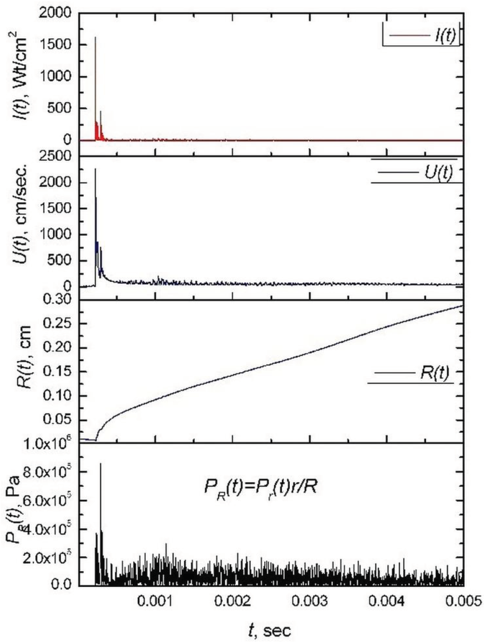
Along with the obtained estimates of the total energy of the emitted acoustic pulse, it is of interest to try to solve the inverse problem – to restore the dynamics of the bubble according to acoustic emission data. The theoretical basis is a formula for the distribution of pressure in the radiated wave from a spherical bubble as a source of monopole radiation, which can be written in the form [3]
where . Solving a nonlinear differential equation with respect to the function R(t), while considering the function P(t) known on the basis of experimental data in the received acoustic pulse, it is possible to calculate the function R(t), the velocity of the bubble wall U(t) and the intensity in the acoustic wave
Figure 19 shows these dependencies, which show that the acoustic data can reproduce the function R(t), which is consistent with the characteristic dependencies R(t) obtained from direct measurements of optical breakdown images at the late stages of its evolution.
4. Discussion of the Results
The main attention in the article was focused on the description of experimental methods and theoretical foundations that allow obtaining and analyzing experimental data on the effective parameters of microinhomogeneous liquids. Real liquids always contain phase inclusions, among which bubbles are the most significant for changing the properties of liquids. Theoretical estimates of the effective parameters of such bubble liquids are carried out in the article. All calculations were carried out in the framework of a homogeneous approximation, while calculations of bubble dynamics were used in the framework of a linear approximation to analyze the complex effective compressibility of a microinhomogeneous liquid. The resonant and relaxation (thermal and diffusion) characteristics of the bubbles, as well as their size distribution, were taken into account.
Previously conducted studies of the distribution of bubbles in typical real liquids (including seawater), allowed in this article to use the model function of bubble size distribution (28) to calculate the effective compressibility (11) and on this basis to obtain estimates for the absorption coefficient and the speed of sound , Equations (21) and (22), valid for sufficiently high concentrations of bubbles. The article did not have the opportunity to discuss the limits of applicability of the approximations made, but the authors, when conducting the analysis, understood the need to take into account the effects of multiple scattering and overlap of sound scattering cross sections at high concentrations of bubbles, and therefore all calculations were carried out in areas where these effects should not be significant.
The effective nonlinear parameter of a microinhomogeneous liquid was estimated under the assumption that the main contribution is made by the nonlinearity of radially symmetric bubble pulsations, the contribution of which differs for bubbles with different sizes. In this regard, it was important to take into account the dimensional effects near the monopole resonance and relaxation near the "second resonance" – the maximum compressibility when the bubble size coincides with the heat wave length, which led to the general formula (26). The estimates of the nonlinearity parameter obtained on this basis and measured experimentally by the methods analyzed in Section 2.1 showed the similarity of the results obtained, which is illustrated by the graphs in Figure 6, Figure 7 and Figure 8 and in Figure 9. Here attention should be paid to the practicality of using the nonlinear acoustic probe described in the article using a parametric emitter in marine research. The probe allows you to obtain a fine structure of water with high spatial resolution.
The calculation of the tensile strength of a liquid is usually carried out taking into account the theory of thermal heterophase fluctuations and the analysis of the size composition of the nuclei. In the article, we took as a basis the Equation (29) obtained in [41] for a pure liquid. However, it was not difficult to generalize the Equation (29) also to a microinhomogeneous liquid. As a result, it was possible to link various characteristics of a microinhomogeneous liquid with simple formulas. Such a phenomenological approach allowed us to obtain the Equation (31) for cavitation strength , which at low concentrations gives the tensile strength of a pure liquid, and at high concentrations of bubbles gives the minimum values of Pa. Since the concept of cavitation is a rather multilateral phenomenon, which is characterized by various approaches to measuring cavitation strength, this article in Section 2.4 gives a small overview of theoretical estimates of alternative approaches to the cavitation threshold based on the effects of rectified heat transfer and rectified gas diffusion, which in conditions of gas saturation of a liquid can lead to a sharp decrease in cavitation thresholds, which is illustrated in Figure 3 and in Figure 4. Later in Section 2.7, the dependence of the cavitation threshold on various criteria for detecting a discontinuity in seawater was studied: by the nonlinearity of the radiated power curve at the frequency of the radiated signal, by the second harmonic, by the total higher harmonics, as well as by subharmonics. Two cavitation thresholds were identified, of which the first threshold corresponds to the beginning of cavitation, and the second to the beginning of violent cavitation, accompanied by a sharp decrease in acoustic impedance. In the work, from the standpoint of detecting precisely the beginning of cavitation, as the beginning of the discontinuity of the continuity of the liquid and the beginning of the formation of bubbles in the liquid, a threshold was chosen, which can be conditionally considered the cavitation strength of the liquid. Figure 13 shows for the selected cavitation threshold that the cavitation strength of seawater significantly depends on the depth in the subsurface layer up to 6 meters thick, and then the dependence on depth is weakly expressed, which indicates a connection with the presence of gas bubbles, always present in the subsurface layer, well shown in Figure 9.
Unfortunately, it was not possible to measure cavitation strength by acoustic methods below a depth of 14 meters due to significant experimental difficulties in creating cavitation at the ultrasound frequencies used. In connection with this circumstance, the optical breakdown in the liquid was studied and the connection with the cavitation strength was established. The obtained dependences of the sound pressure P at the leading edge and the spectral characteristics of the generated acoustic pulse on the energy E of the laser pulse causing the optical breakdown allowed us to estimate the dynamics of the breakdown region based on acoustic emission data.
Comparing the data obtained for the cavitation strength of water presented in Figure 13 and in Figure 19, one can see fairly close values of experimental measurements of cavitation strength obtained by acoustic method and using laser breakdown. The lower graph of Figure 19 shows an estimate of the pressure on the wall of the cavity at which a breakdown occurs, which turned out to be close to the value of the cavitation strength in seawater at a depth of 5 meters.
Here we assume that such a coincidence is not accidental, namely, the cavitation strength of liquids in the case of vapor cavitation, when there are no gas bubbles, will correspond to the boiling temperature threshold of the liquid when it is locally overheated by a laser pulse, provided that the corresponding overheating is associated with the cavitation strength by dependence , where corresponds to the slope of the phase equilibrium curve of the liquid- vapor.
This assumption needs to be thoroughly verified, especially at high hydrostatic pressures corresponding to great depths for seawater, for which, according to Figure 2, there is a strong dependence of cavitation strength on depth. The use of an independent assessment of the cavitation threshold of a liquid using a laser breakdown of a liquid may be of practical importance if it is necessary to measure cavitation strength at great depths in marine conditions where it is extremely difficult to realize high acoustic pressure values using traditional radiators. The use of optical cavitation would be a way out of this situation due to the use of a completely different mechanism of discontinuity of the medium – induced laser pulse boiling, which corresponds in all parameters to the formation of a critical nuclei of a new phase and its further growth in the supercritical region to macroscopic dimensions. It is this mechanism that is usually implemented during cavitation in the absence of gas bubbles, which significantly facilitate the rupture of the liquid.
5. Conclusion
In the work, within the framework of the homogeneous approximation of a microinhomogeneous liquid, studies of the effective parameter of acoustic nonlinearity and cavitation strength of a liquid with bubbles were carried out. The analysis used data on the bubble size distribution function in seawater, which were written in the form of a formula that simplifies the calculation of the effective parameters of a microinhomogeneous liquid.
The relationship of the acoustic nonlinearity parameter, cavitation strength, absorption coefficient and velocity dispersion with the bubble size distribution function was established and typical values of these parameters were calculated for different gas contents in water in the form of bubbles.
Experimental measurements of the acoustic nonlinearity parameter and the cavitation strength of seawater at various depths have been carried out, which are consistent with theoretical estimates. The interrelation of these characteristics for seawater is shown.
Due to the difficulties of measuring cavitation strength by acoustic methods, other methods are being sought. It is proposed to use an optoacoustic method associated with the use of laser radiation, which causes optical breakdown of optical cavitation, accompanied by a strong sound generation effect. The connection between optical breakdown thresholds and acoustic cavitation thresholds has been established, which can later be used to identify cavitation thresholds at high static pressures (at great depths in the sea), where the use of acoustic emitters is extremely difficult.
Author Contributions
Conceptualization, AB, VB; Methodology, AB, VB, IK; Software, AB, ES; Validation, AB, VB, IK; Formal Analysis, AB, VB; Investigation, AB, VB, IK; Resources, VB, AB; Data Curation, AB, VB, ES; Writing – Original Draft Preparation, AB, VB. ES; Writing – Review & Editing, AB, VB; Visualization, AB, VB, ES; Supervision, AB, VB; Project Administration, AB; Funding Acquisition, VB. AB –A.V. Bulanov, ES – E.S. Sosedko, VB – V.A. Bulanov, IK – I.V. Korskov.
Funding
The work was carried out with the support of the grant of the Russian Science Foundation No. 22-22-00499.
Conflicts of Interest
The authors declare no conflict of interest.
References
- Beyer, R.T. Parameter of nonlinearity in fluids. J. Acoust. Soc. Amer. 1960, 32, 719–721. [Google Scholar] [CrossRef]
- Novikov, B.K.; Rudenko, O.V.; Timoshenko, V.I. , Nonlinear Underwater Acoustics, New York: American Institute of Physics, 1987.
- Naugolnykh, K.A.; Ostrovsky, L.A. , Nonlinear Wave Processes in Acoustics, Cambridge: University Press, 1998. 298 p.
- Bjorno, L. Finite-Amplitude Wave Propagation through Water-Saturated Marine Sediments. Acustica 1977, 38, 195–200. [Google Scholar]
- Hamilton, M.F.; Fenlon, F.H. , Parametric acoustic array formation in dispersive fluids. J. Acoust. Soc. Amer. 1984, 76, 1474–1492. [Google Scholar] [CrossRef]
- Apfel, R.E. The effective nonlinearity parameter for immiscible liquid mixtures. // J. Acoust. Soc. Amer. 74, No.6, p.1866-1868, 1983.
- Nazarov, V.E.; Ostrovsky, L.A.; Soustova, I.A.; Sutin, A.M. , Nonlinear acoustics of micro-inhomogeneous media. Phys. Earth and Planetary Inter. 1988, 34, 94–98. [Google Scholar] [CrossRef]
- Neppiras, E.A. , Acoustic cavitation. Phys. Reports. 1980, 61, 159–251. [Google Scholar] [CrossRef]
- Leighton, T. G. The Acoustic Bubble. Academic: SanDiego, 1994. [Google Scholar]
- Karpov, S.; Prosperetti, A.; Ostrovsky, L. , Nonlinear wave interactions in bubble layers. J. Acoust. Soc. Am. 2003, 113, 1304–1316. [Google Scholar] [CrossRef] [PubMed]
- Brekhovskikh, L.M.; Lysanov, Yu.P. , Fundamentals of ocean acoustics. Berlin, N.Y.: Springer, 1982, 250 p.
- Wu, J. , Bubbles in the near-surface ocean: Their various structures. J. Phys. Oceanogr. 1994, 24, 1955–1965. [Google Scholar] [CrossRef]
- Baschek, B.; Farmer, D.M. , Gas Bubbles as Oceanographic Tracers. J. Atmosph. Oceanic Technol. 2010. 27.
- Akulichev, V.A.; Bulanov, V.A. Measurements of bubbles in sea water by nonstationary sound scattering. J. Acoust. Soc. Amer. 2011, 130, 3438–3449. [Google Scholar] [CrossRef] [PubMed]
- Liu, R.; Li, Z. The effects of bubble scattering on sound propagation in shallow water. J. Mar. Sci. Eng. 2021, 9, p.1441. [CrossRef]
- Akulichev, V.A.; Bulanov, V.A. The bubble distribution and acoustic characteristics of the subsurface sea layer. Proc. Mtgs. Acoust. 2015, 24, 045003. [Google Scholar]
- Grelowska, G.; Kozaczka, E. Nonlinear properties of the Gotland deep – Baltic Sea. Arch. Acoust. 2015, 40, 595–600. [Google Scholar] [CrossRef]
- Apfel, R.E. Acoustic cavitation. Methods Exp. Phys. 1981, 19, 355–411. [Google Scholar]
- Akulichev, V.A. Cavitation nuclei and thresholds of acoustic cavitation in ocean water. In book: Bubble Dynamics and Interface Phenomena, Ed. J.R. Blake, J.M. Boulton-Stone, N.H. Thomas. Kluwer Academic Publishers: The Netherlands, 1994. pp. 171–178.
- Caupin, F.; Herbert, E. Cavitation in water: a review. C. R. Physique. 2006, 7, 1000–1017. [Google Scholar] [CrossRef]
- Sette, D.; Wanderling, F. Nucleation by cosmic rays in ultrasonic cavitation. Phys. Rev. 1962, 1962. 125, 409. [Google Scholar] [CrossRef]
- Akulichev, V.A.; Il’ichev, V.I. Thresholds of acoustic cavitation in sea water in various areas of the World ocean. Phys. Acoust. 2005, 51, 167–179. [Google Scholar] [CrossRef]
- Bulanov, V.A. Acoustical nonlinearity of microinhomogeneous liquids. In Advances in nonlinear acoustics. Ed. H.Hobaek, World Scientific: Singapore-London-New Jersey, 1993, pp. 674–679.
- Lauterborn, W.; Kurz, T. Physics of bubble oscillations. Rep. Prog. Phys. 2010, 73, 106501. [Google Scholar] [CrossRef]
- Kurz, T; Kroninger, D; Geisler, R; Lauterborn, W. Optic cavitation in an ultrasonic field. Phys. Rev. E 2006, 74, 066307. [Google Scholar] [CrossRef] [PubMed]
- Padilla– Martinez, J.P.; Berrospe– Rodriguez, C; Aguilar, G. ; Ramirez– San– Juan, J. C.; Ramos– Garcia, R. Optic cavitation with CW lasers: A review. Phys.Fluids. 2014, 26, 122007. [Google Scholar] [CrossRef]
- Cremers, D.A.; Radziemski, L.J. Handbook of Laser– Induced Breakdown Spectroscopy, John Wiley& Sons: New York, 2006, p.282.
- Musazzi, S.; Perini, U. Laser-Induced Breakdown Spectroscopy. Springer Series in Optical Sciences 182, Springer-Verlag: Berlin Heidelberg, 2014, 575 p.
- Kurz, T.; Wilken, T.; Kroninger, D; Wimann, L. ; Lauterborn, W. Transient dynamics of laser– induced bubbles in an ultrasonic field. AIP Conf. Proc. 2008, 1022, 221–224. [Google Scholar]
- Kudryashov, S.I.; Lyon, K.; Allen, S.D. Photoacoustic study of relaxation dynamics in multibubbles systems in laser– superheated water. Phys. Rev. E 2006, 73, 055301. [Google Scholar] [CrossRef]
- Taylor, R.S.; Hnatovsky, C. Growth and decay dynamics of a stable microbubble produced at the end of a near– field scanning optical microscopy fiber probe. J. Appl. Phys. 2004, 95, 8444. [Google Scholar] [CrossRef]
- Byun, K.T.; Kwak, H.Y.; Karng, S.W. Bubble evolution and radiation mechanism for laser– induced collapsing bubble in water. Jpn. J. Appl. Phys. 2004, 43, 6364–6370. [Google Scholar] [CrossRef]
- Akulichev, V.A.; Bulanov, V.A. Acoustic study of small-scale heterogeneities in the marine environment. POI FEB RAS: Vladivostok. 2017. 414 p., https://www.poi.dvo.ru/node/470.
- Bulanov, V.A.; Korskov, I.V.; Popov, P.N. V.; Popov, P.N. Measurements of the nonlinear acoustic parameter of sea water via a device using reflected pulses. Instrum. Exp. Tech. 2017, 60, 414–417. [Google Scholar] [CrossRef]
- Akulichev, V.A.; Bulanov, V.A. Spectrum of gas bubbles and possibilities of acoustic spectroscopy in the surface layer of the ocean. Dokl. Earth Sci. 2012, 446, 1112–1115. [Google Scholar] [CrossRef]
- Garrett, C.; Li, M.; Farmer, D. The Connection between bubble size spectra and energy dissipation rates in the upper ocean. J. Phys. Ocean. 2000, 30, 2163–2171. [Google Scholar] [CrossRef]
- Farmer, D.; Vagle, S. Wave induced bubble clouds in the upper ocean. J. Geophys. Res. 2010, 115, C12054. [Google Scholar]
- Bulanov, V.A.; Bugaeva, L.K.; Storozhenko, A.V. On sound scattering and acoustic properties of the upper layer of the sea with bubble clouds. J. Mar. Sci. Eng. 2022, 10, 872. [Google Scholar] [CrossRef]
- Deane, G.B.; Preisig, J.C.; Lavery, A.C. The suspension of large bubbles near the seasurface by turbulence and their role in absorbing forward-scattered sound. IEEE Journ.of Oceanic Eng. 2013, 38, 632–641. [Google Scholar] [CrossRef]
- Liu, R.; Li, Z. The Effects of Bubble Scattering on Sound Propagation in ShallowWater. J. Mar. Sci. Eng. 2021, 9, 1441. [Google Scholar] [CrossRef]
- Sehgal, C.M. Non-linear ultrasonics to determine molecular properties of pure liquids. Ultrasonics 1995, 33, 155–161. [Google Scholar] [CrossRef]
- Akulichev, V.A.; Zhukov, V.A.; Tkachev, L.G. Ultrasonic bubble chambers. Phys. Elem. Part. At. Nucl. 1977, 8, 580–629. [Google Scholar]
- Eller, A. Effects of diffusion on gaseous cavitation bubbles. J. Acoust. Soc. Amer. 1975, 57, 1374–1379. [Google Scholar] [CrossRef]
- Hsieh, D.Y.; Plesset, M.S. Theory of rectified diffusion of mass into gas bubbles. J. Acoust. Soc. Amer. 1961, 33, 206–215. [Google Scholar] [CrossRef]
- Finch, R.D.; Neppiras, E.A. Vapour dynamics. J. Acoust. Soc. Amer. 1973, 53, 1402–1410. [Google Scholar] [CrossRef]
- Wang, T.G. Rectified heat transfer. J. Acoust. Soc. Amer. 1974, 56, 1131–1143. [Google Scholar] [CrossRef]
- Crum, L.A.; Cary, M.H. Generalired equations for rectified diffusion, J. Acoust. Soc. Amer. 1982, 72, 483–487. [Google Scholar] [CrossRef]
- Akulichev, V.A.; Bulanov, V.A.; Polovinka, Yu.A. Rectified gas diffusion and rectified heat transfer at vapour-gas babble dynamics in a sound field. In. Proc. Ultrason. Int. Symp. 1985, 85, 249–253. [Google Scholar]
- Del Grosso, V.A.; Mader, C.W. Speed of sound in pure water. J. Acoust. Soc. Am. 1972, 52, 1442–1446. [Google Scholar] [CrossRef]
- Fofonoff, N.P.; Millard, R.C. Jr. Algorithm for computation of fundamental properties of seawater. UNESCO Technical papers in Marine Science. 1983. No. 44.
- Bukin, O.A.; Salyuk, P.A.; Maior, A.Yu.; et al. The use of laser spectroscopy methods in the Investigation of the carbon cycle in the jcean. Atmos. Ocean. Opt. 2010, 23, 328–33. [Google Scholar] [CrossRef]
- Ilyin, A.A.; Nagorny, I.G.; Bukin, O.A.; et al. Features of development of optical breakdown on an inclined fluminum surface. Tech. Phys. Lett. 2012, 38, 975–978. [Google Scholar] [CrossRef]
- Bulanov, A.V. , Nagorny, I.G. Acoustic effects at interaction of laser radiation with a liquid accompanied by optical breakdown. AIP Conf. Proc. 2012, 351–354. [Google Scholar]
- Bulanov, A.V.; Nagorny, I. G.; Sosedko, E.V. Spectroscopic features of laser-induced breakdown in water and aqueous solutions in ultrasonic field. Tech. Phys. Lett. 2017, 43, 753–755. [Google Scholar] [CrossRef]
- Bulanov, A.V. , Nagorny, I. G.; Sosedko, E.V. А study of the optical and acoustic spectral characteristics by laser breakdown of water in an ultrasonic field. Tech. Phys. Lett. 2019, 45, 1200–1203. [Google Scholar] [CrossRef]
- Bulanov, A.V.; Sosedko, E.V. Оpto-acoustic effects by laser breakdown of seawater in an ultrasonic field. Dokl. Earth Sci. 2020, 491, 183–186. [Google Scholar] [CrossRef]
- Bulanov, A.V. Using of ultrasound in automated laser induced breakdown spectroscopy complex for operational study of spectral characteristics of seawater of carbon polygons. Bull. Russ. Acad. Sci. Phys. 2022, 86, S32–S36. [Google Scholar] [CrossRef]
Figure 1.
Dependence for water at 200C at different frequencies of the acoustic field.
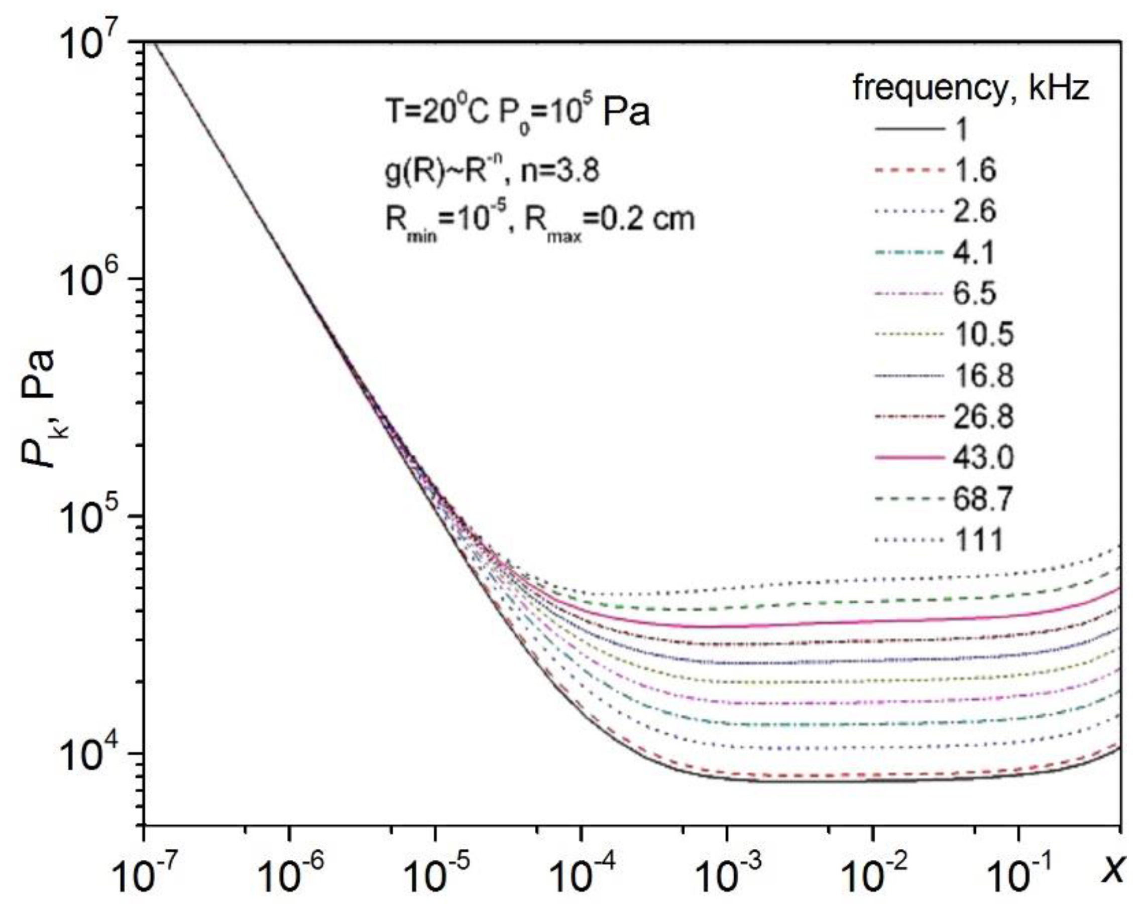
Figure 2.
Dependence at different hydrostatic pressure.
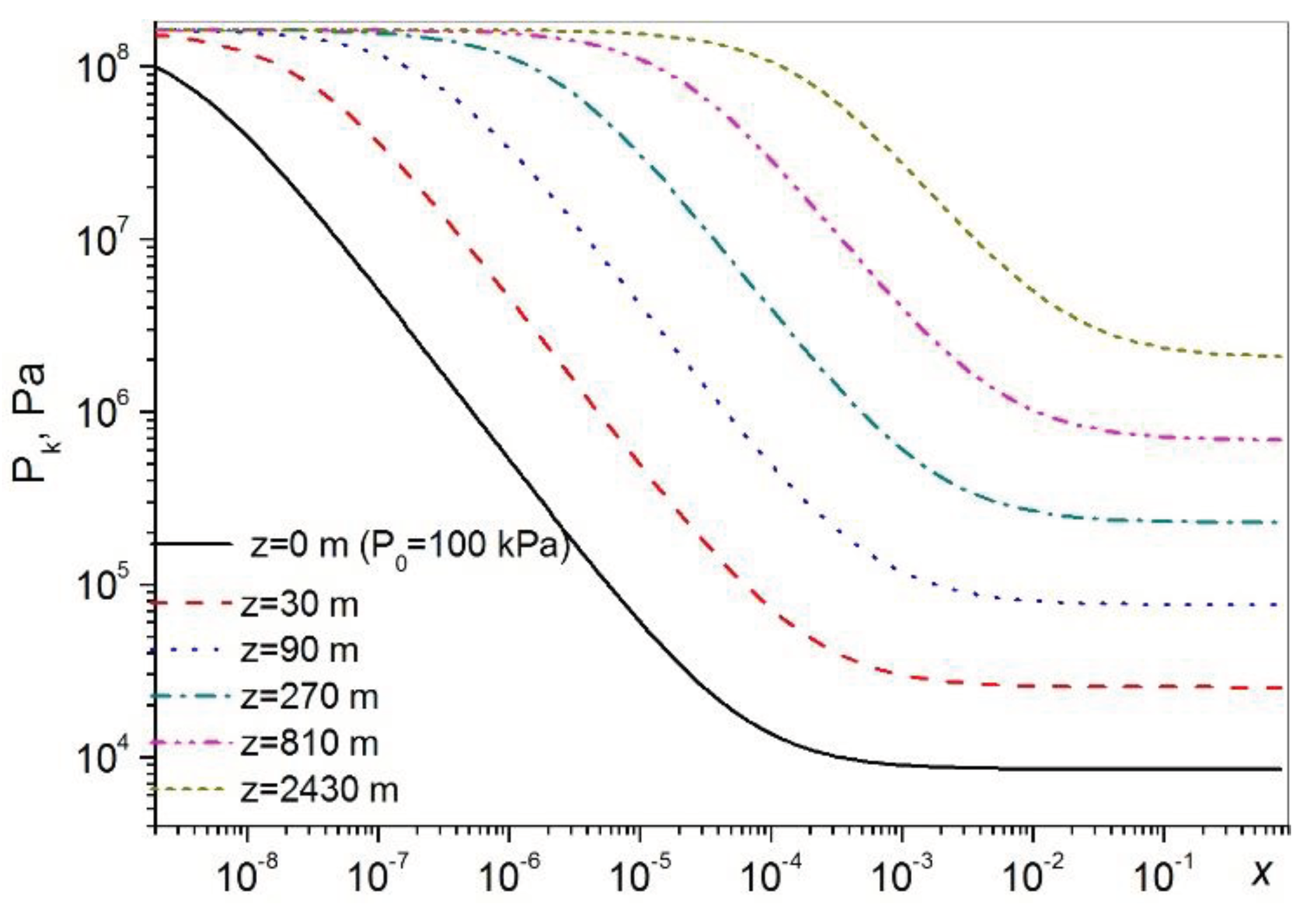
Figure 3.
Thresholds for the growth of vapor-gas bubbles in water at frequencies of 50 kHz - (a) and 500 kHz - (b), the concentration of dissolved gas in water is below equilibrium concentration at different temperatures .
Figure 3.
Thresholds for the growth of vapor-gas bubbles in water at frequencies of 50 kHz - (a) and 500 kHz - (b), the concentration of dissolved gas in water is below equilibrium concentration at different temperatures .
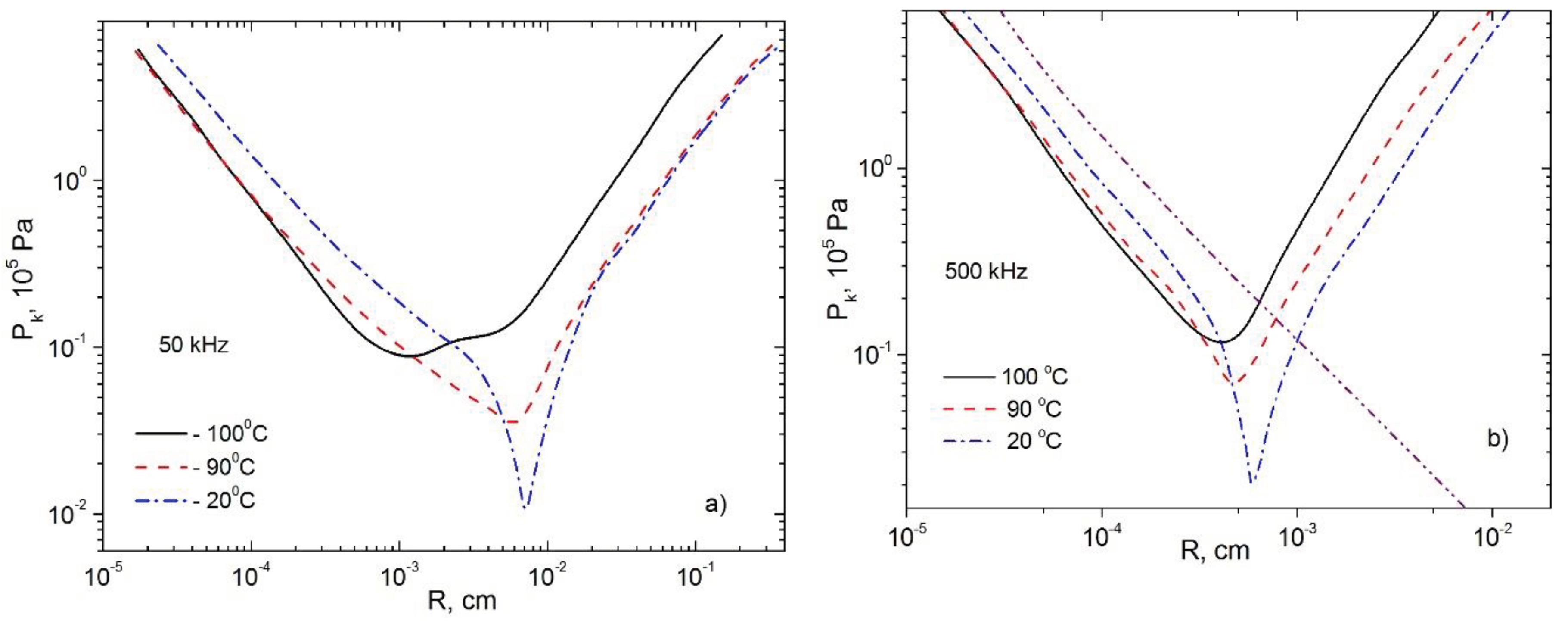
Figure 4.
Thresholds for the growth of vapor-gas bubbles in water at frequencies of 0.5 kHz and 5 kHz at different concentrations of dissolved gas in water (solid lines - dashed lines - ).
Figure 4.
Thresholds for the growth of vapor-gas bubbles in water at frequencies of 0.5 kHz and 5 kHz at different concentrations of dissolved gas in water (solid lines - dashed lines - ).
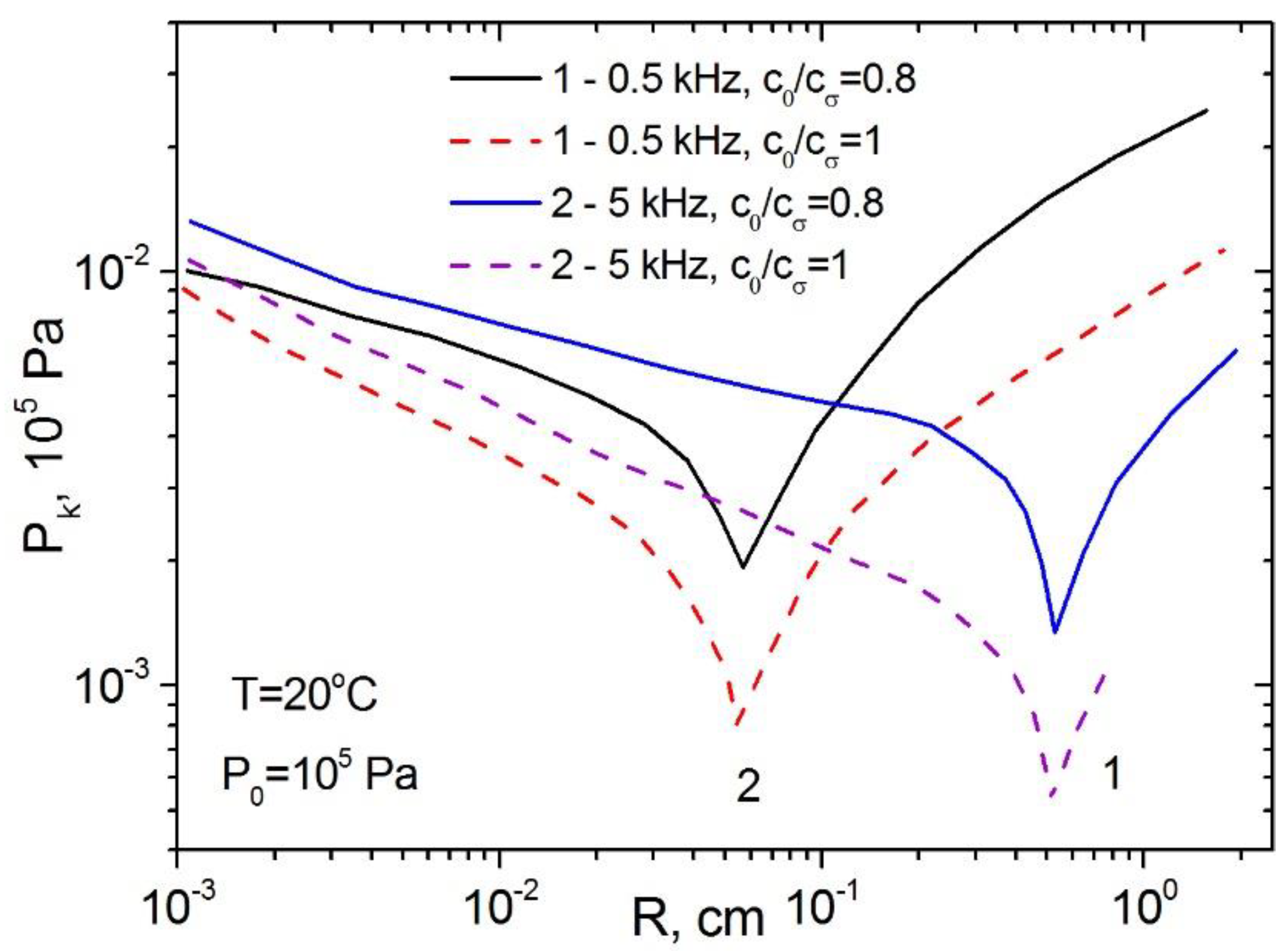
Figure 5.
Functional diagram of the probe for measuring the nonlinear acoustic parameter of water (a) and the frequency spectrum on the receiving hydrophone (b) when emitting a biharmonic signal of 698 kHz and 716 kHz: 1 – path of generation and emission of parametric pulses; 2 – switch of radiation-reception signals; 3 – parametric emitter; 4 – reflecting plate; 5 – selective difference frequency signal amplifier; 6 – depth sensor; 7 – two-channel ADC; 8 - computer.
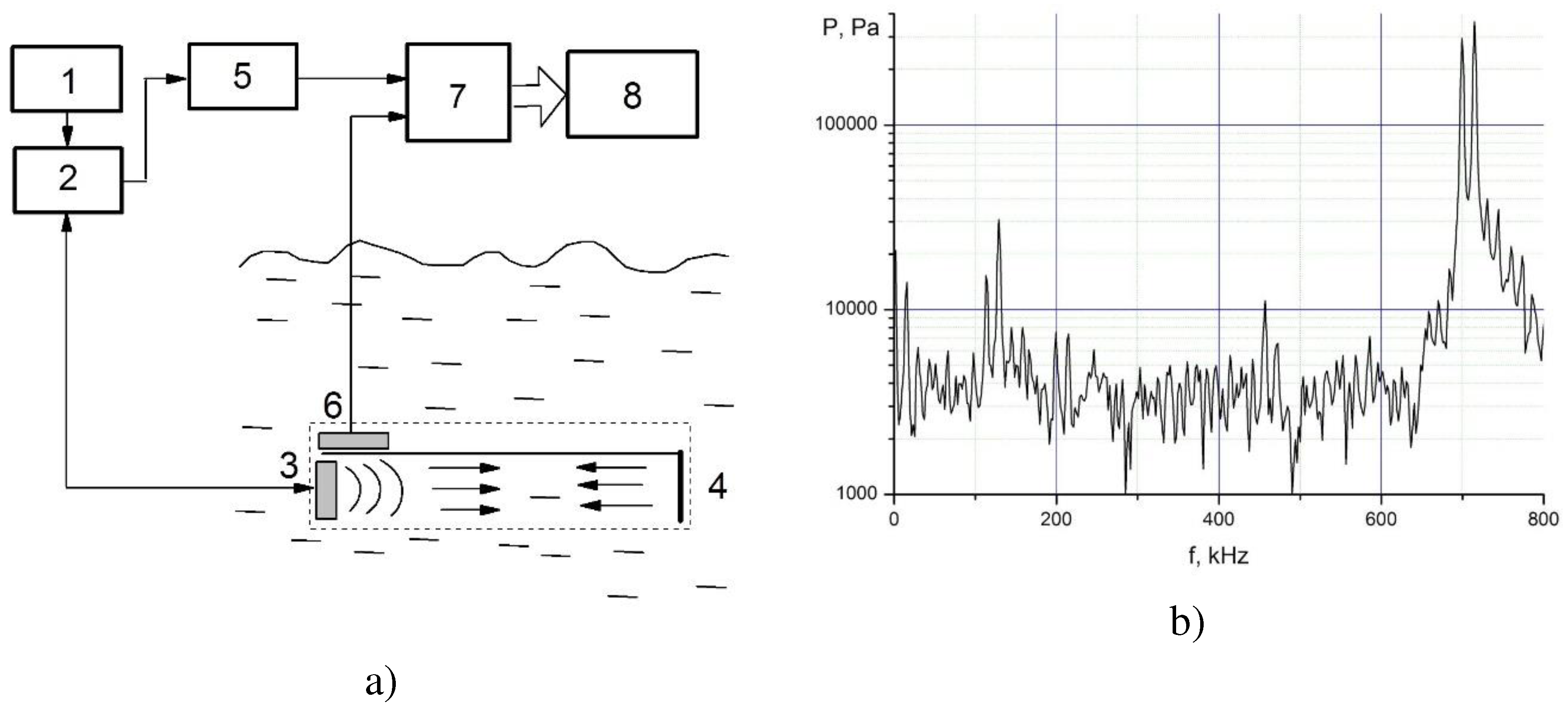
Figure 6.
Nonlinear parameter of the subsurface layer of the subarctic waters of the North Pacific (averaged data).
Figure 6.
Nonlinear parameter of the subsurface layer of the subarctic waters of the North Pacific (averaged data).
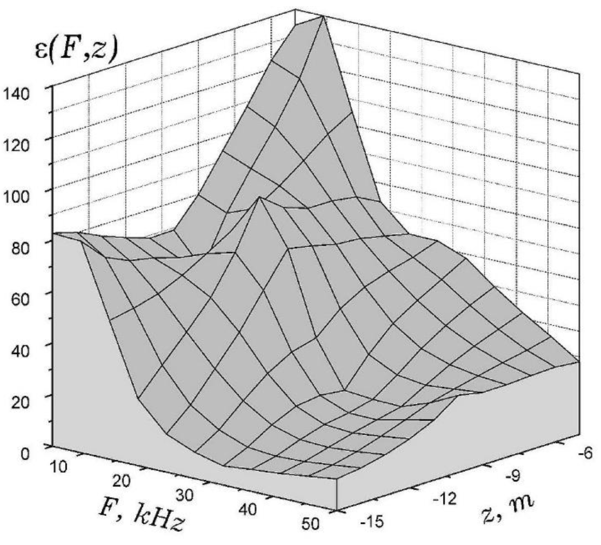
Figure 7.
The dependences of the nonlinear parameter on the depth , significantly exceeding the calculated dependences for pure water and indicating the presence of an additional contribution associated with the presence of micro-inhomogeneities in the sea and recorded using the sound scattering coefficient : 1 – temperature ; 2 – ; 3 - at a frequency of 15 kHz (pumping 700 kHz); 4 – at a frequency of 100 kHz.
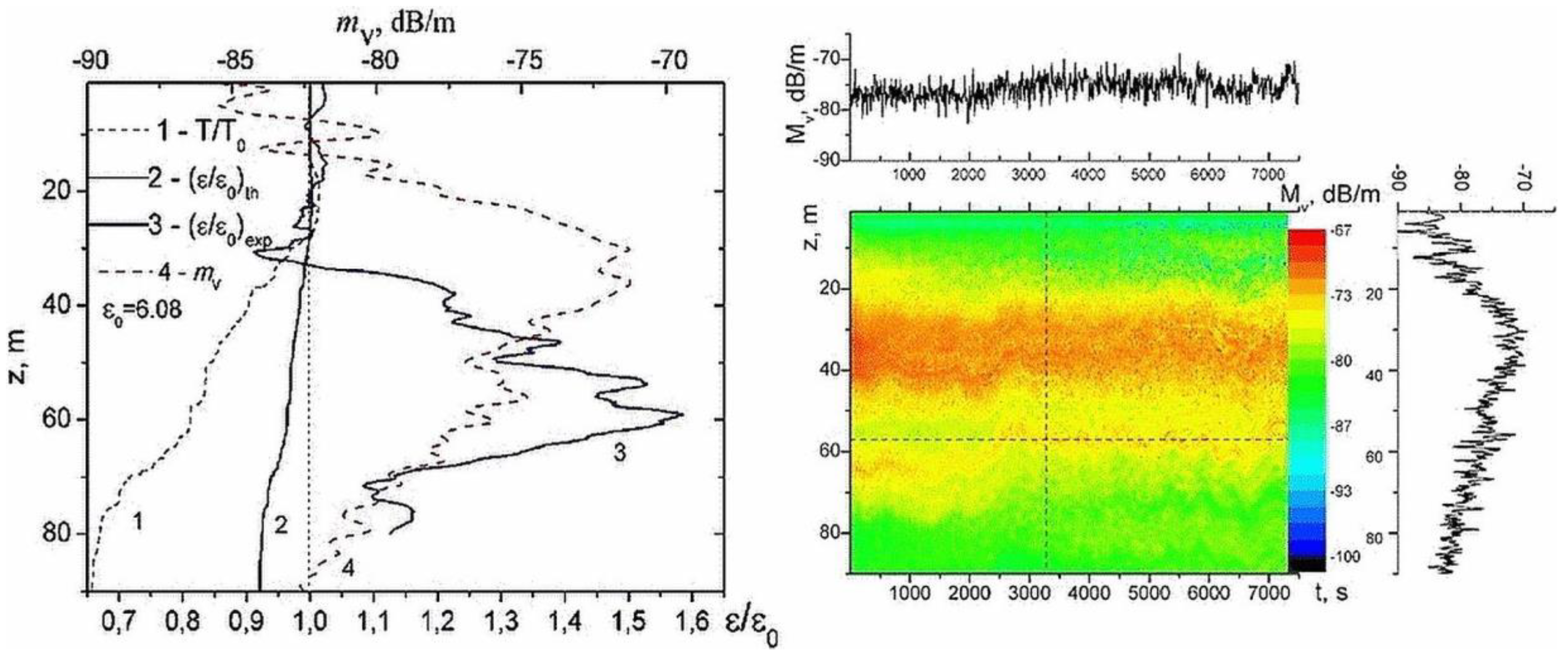
Figure 8.
Dependences of the nonlinearity parameter on the depth in the water area Vityaz Bay (the Sea of Japan) with different sounding: a) - from the surface to a depth of 21 m, b) - from a depth of 21 m upwards.
Figure 8.
Dependences of the nonlinearity parameter on the depth in the water area Vityaz Bay (the Sea of Japan) with different sounding: a) - from the surface to a depth of 21 m, b) - from a depth of 21 m upwards.

Figure 9.
The time change in the near-surface layer of the sea with a sharp change in wind strength and the manifestation of the relationship of acoustic nonlinearity ε, sound absorption α, and bubble distribution in the near-surface layer of the sea (in m-3mkm-1) at a depth of z, marked by a horizontal line in the lower figure.
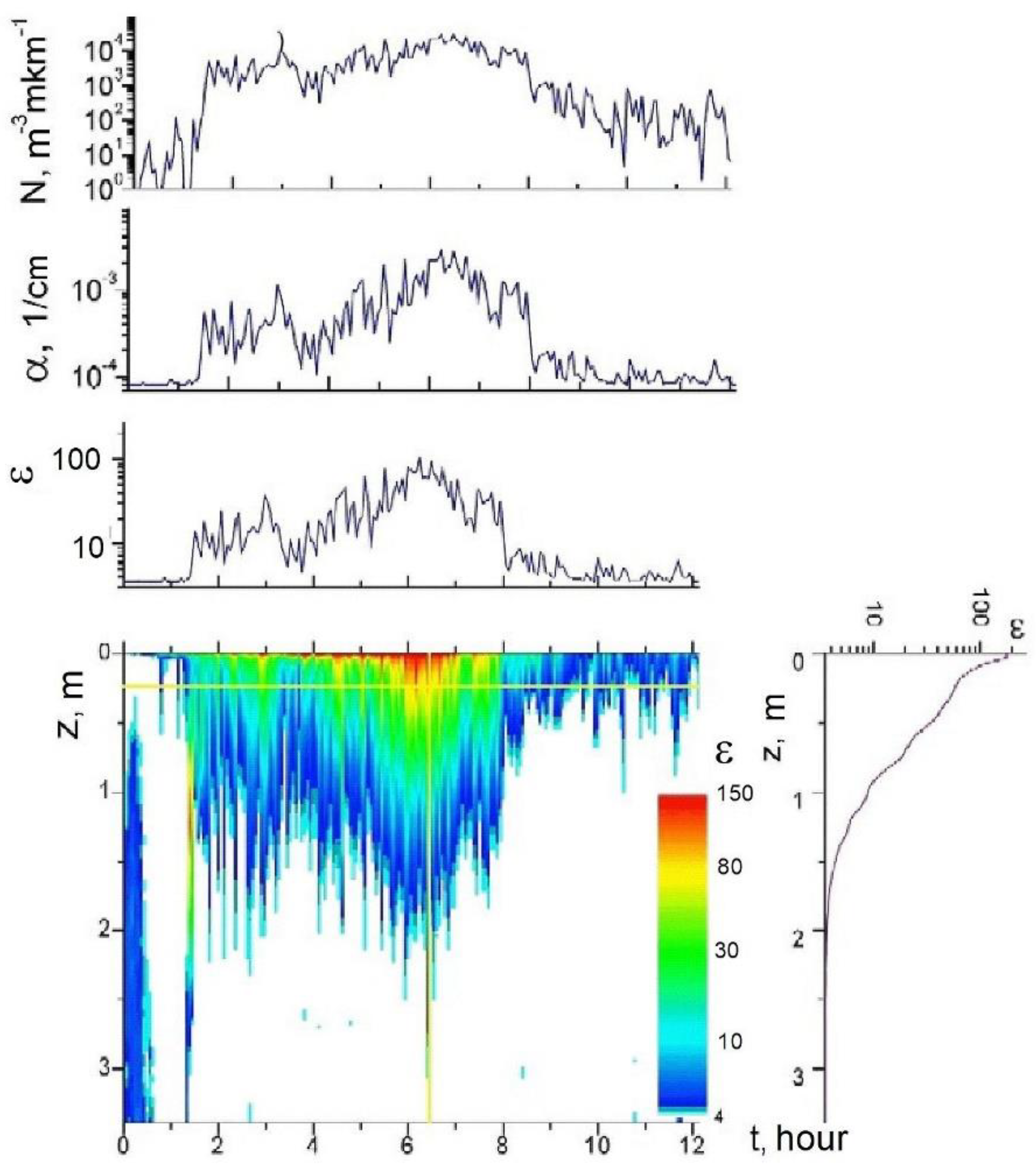
Figure 10.
Dependences on the emitter voltage of the spectral components of acoustic noise: the subharmonic signal , the total higher harmonics and higher harmonics, starting from the 6th harmonic.
Figure 10.
Dependences on the emitter voltage of the spectral components of acoustic noise: the subharmonic signal , the total higher harmonics and higher harmonics, starting from the 6th harmonic.
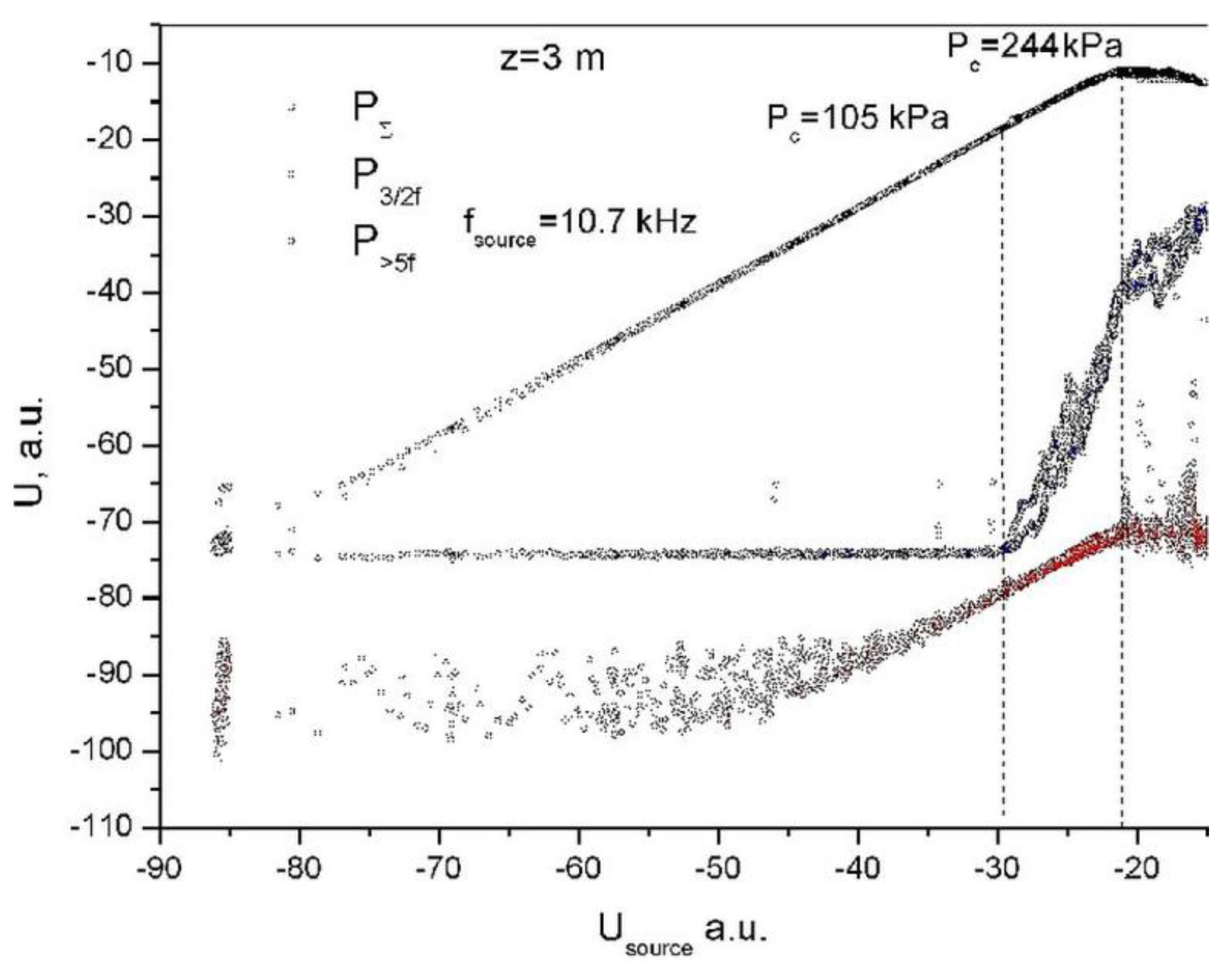
Figure 11.
Dependences on the time of the subharmonic signal , total harmonics in the frequency range from 1 kHz to 1 MHz and higher harmonics , starting from the 6th harmonic.
Figure 11.
Dependences on the time of the subharmonic signal , total harmonics in the frequency range from 1 kHz to 1 MHz and higher harmonics , starting from the 6th harmonic.
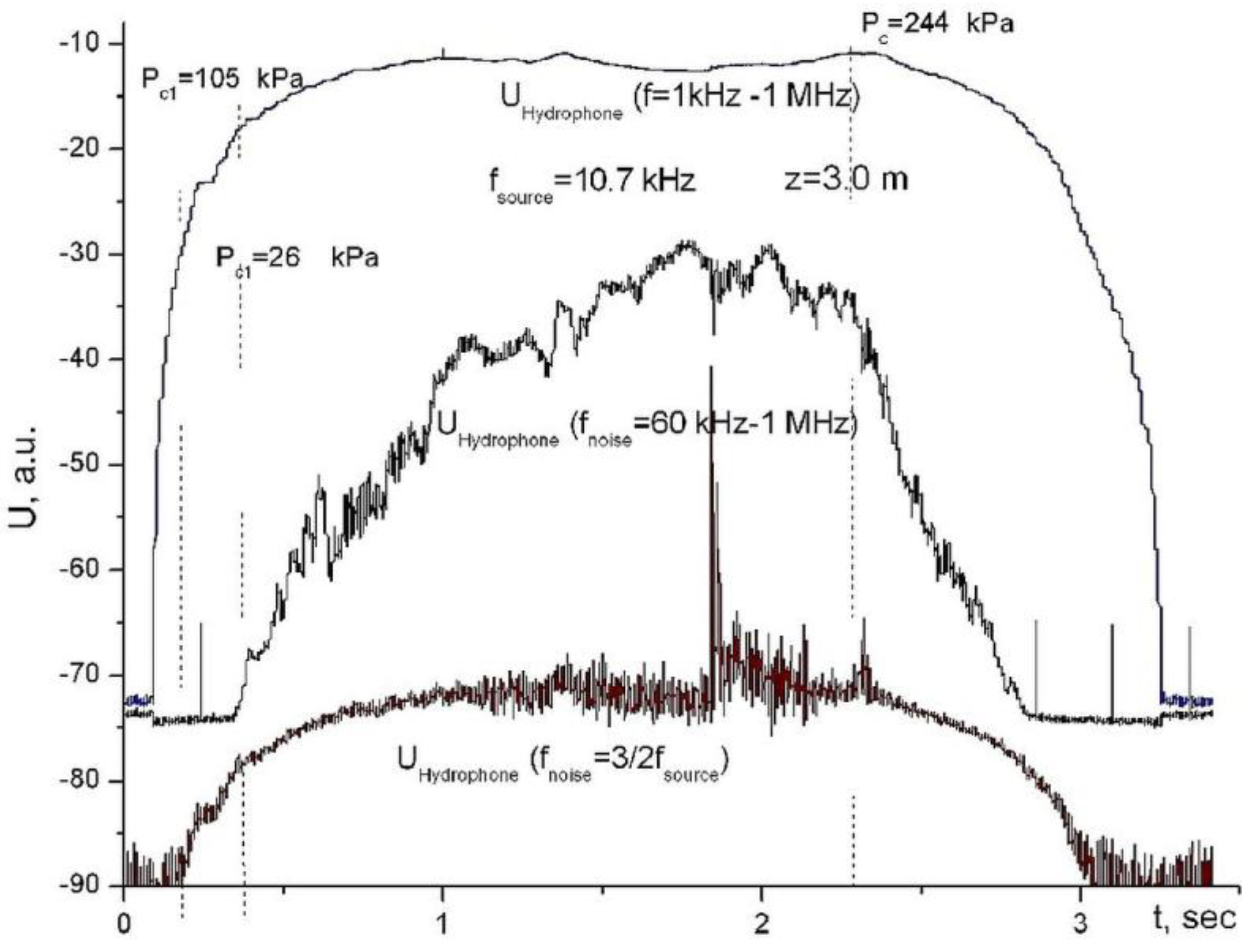
Figure 12.
Distribution of temperature and salinity of seawater depending on depth.
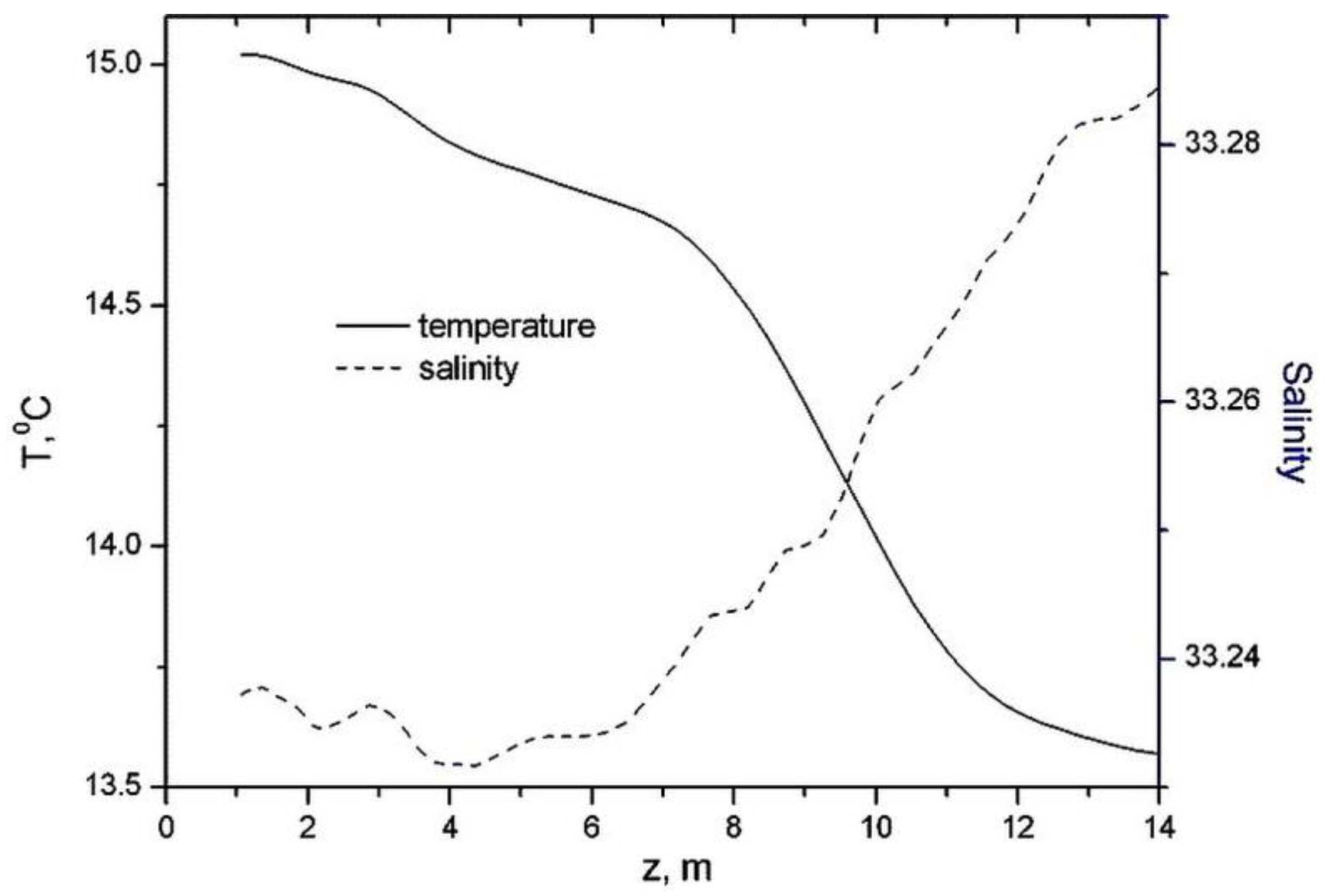
Figure 13.
Cavitation strength of seawater depending on depth.
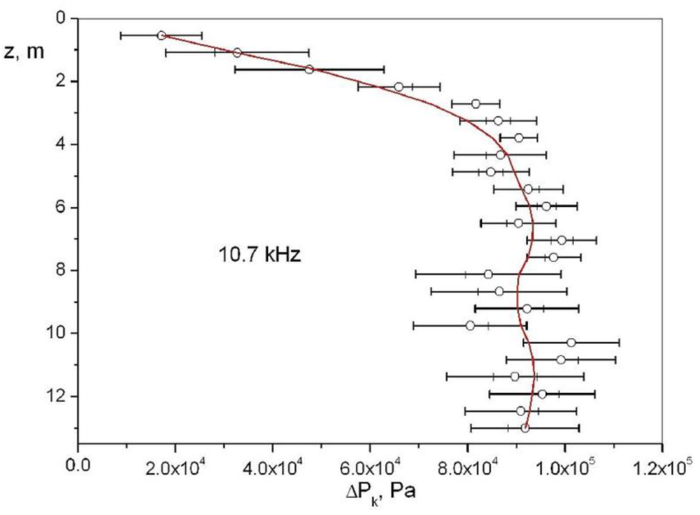
Figure 14.
The scheme of the experiment. 1, 2 – laser, 3 – control pulse switch, 4 – pulse generator of arbitrary shape GSPF 053, 5 – power amplifier type U7-5 or Pioneer GM-A3702, 6 – piezoceramic ultrasonic emitter, 7 – delay generator, 8 – CCD camera, 9 – monochromator, 10 – computer, 11, 12 – rotary mirror and lens, 13 – breakdown area, 14 – collecting lens, 15 – PV6501 oscilloscope, 16 – E20-10 ADC board, 17 – Brüel&Kjær hydrophone type 8103.
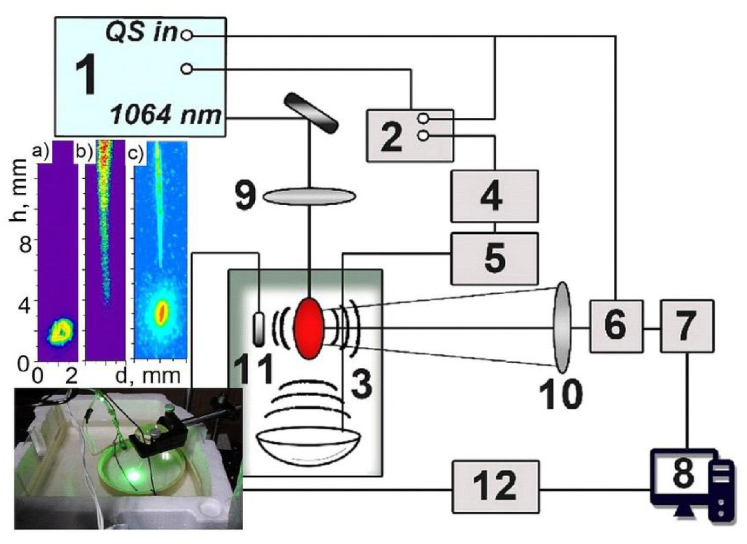
Figure 15.
Acoustic emission spectrum at various separate forms of laser breakdown of water – on the surface and in the water column.
Figure 15.
Acoustic emission spectrum at various separate forms of laser breakdown of water – on the surface and in the water column.
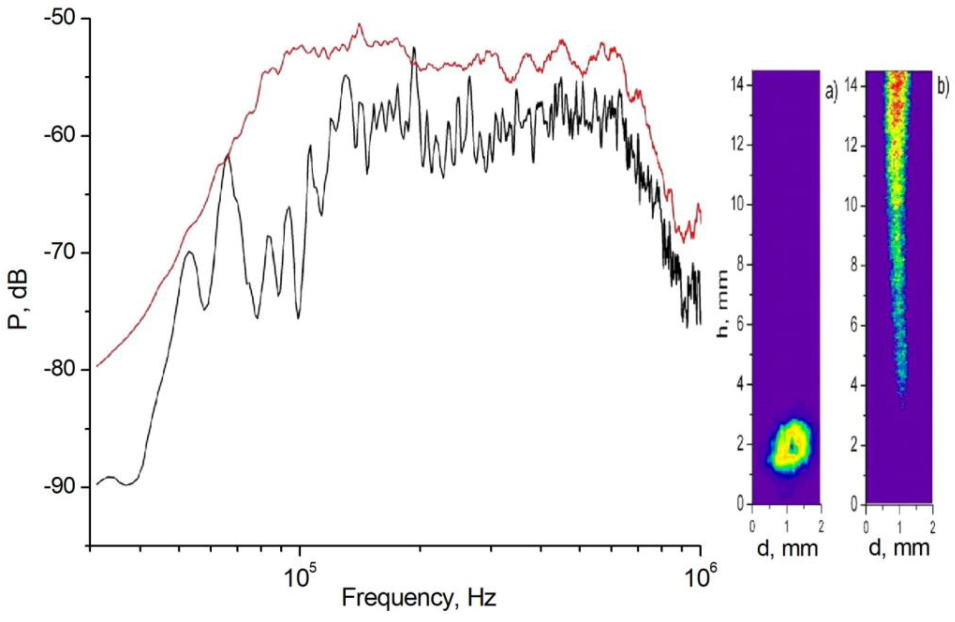
Figure 16.
The shape of the acoustic pulse from the breakdown zone received by the hydrophone in the liquid.
Figure 16.
The shape of the acoustic pulse from the breakdown zone received by the hydrophone in the liquid.
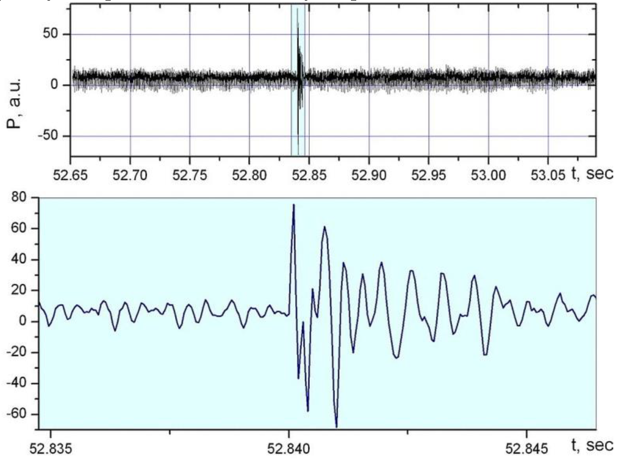
Figure 17.
Features of acoustic emission with an increase in the energy of the laser pulse E.
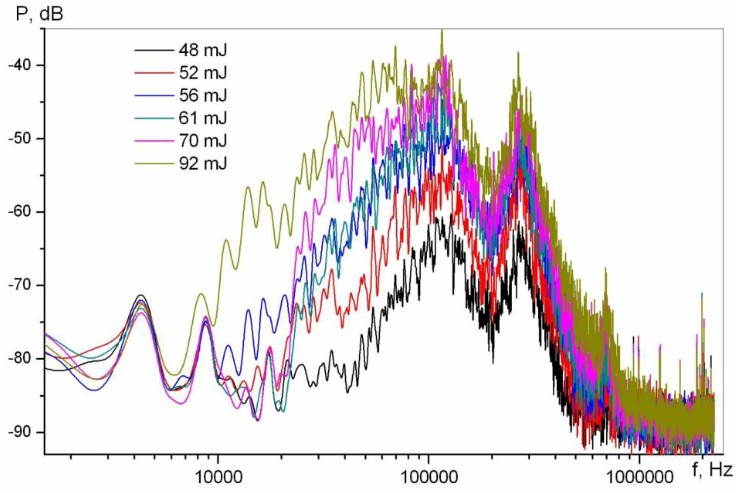
Figure 18.
The dependence of the sound pressure P on the leading edge of the acoustic pulse on the energy E: experimental points, linear approximation by the formula indicated on the graph (solid line) and 96% confidence interval of approximation (dashed lines).
Figure 18.
The dependence of the sound pressure P on the leading edge of the acoustic pulse on the energy E: experimental points, linear approximation by the formula indicated on the graph (solid line) and 96% confidence interval of approximation (dashed lines).
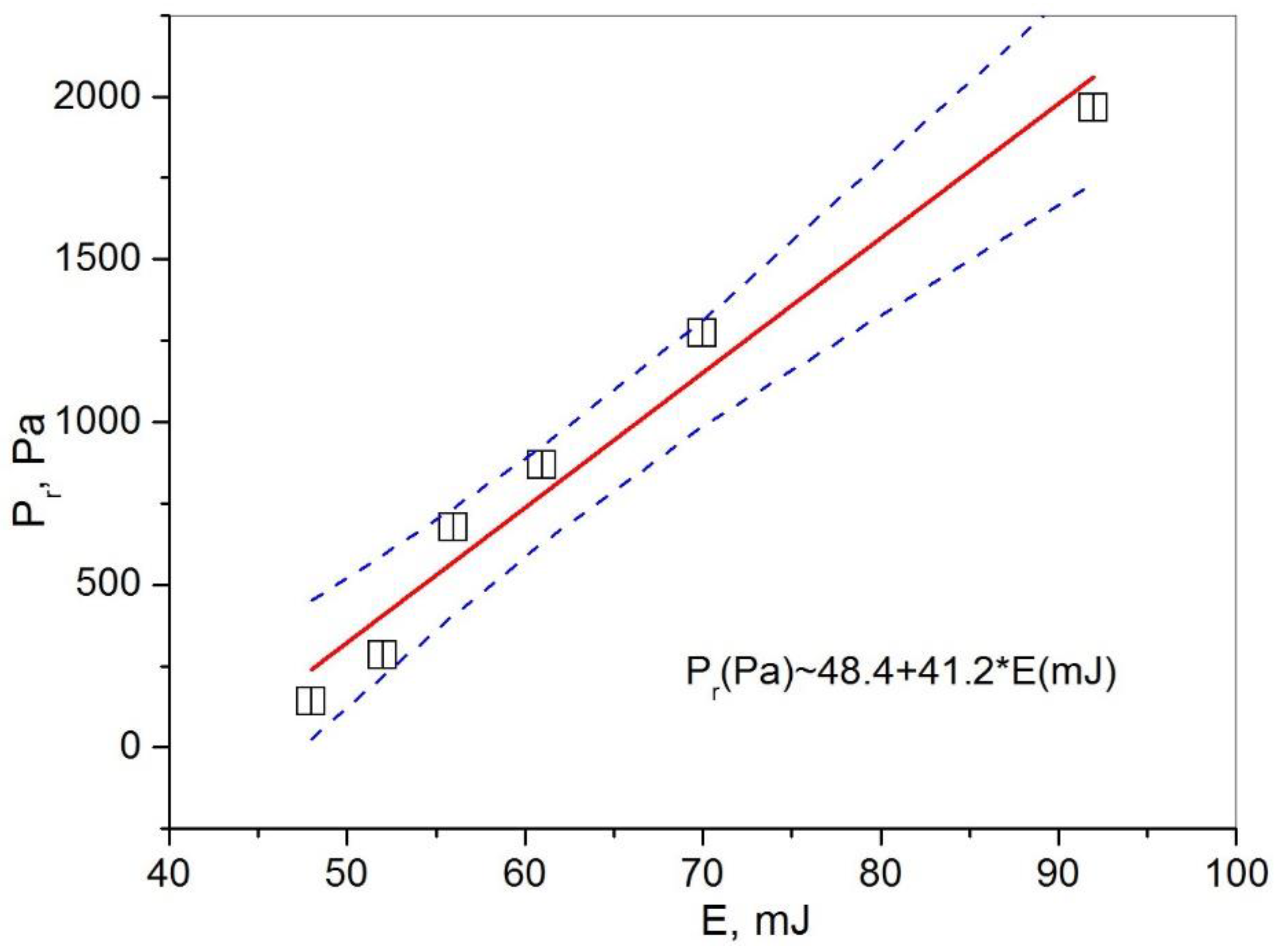
Figure 19.
Acoustic emission and bubble dynamics (from bottom to top): time dependence of pressure P(t) in the received acoustic pulse on the optical breakdown region; function R(t) calculated by formula (35) from data for P(t); function dR(t)/dt, constructed for calculated function R(t); intensity in the emitted acoustic pulse I(t).
Disclaimer/Publisher’s Note: The statements, opinions and data contained in all publications are solely those of the individual author(s) and contributor(s) and not of MDPI and/or the editor(s). MDPI and/or the editor(s) disclaim responsibility for any injury to people or property resulting from any ideas, methods, instructions or products referred to in the content. |
© 2023 by the authors. Licensee MDPI, Basel, Switzerland. This article is an open access article distributed under the terms and conditions of the Creative Commons Attribution (CC BY) license (http://creativecommons.org/licenses/by/4.0/).
Copyright: This open access article is published under a Creative Commons CC BY 4.0 license, which permit the free download, distribution, and reuse, provided that the author and preprint are cited in any reuse.


