

Submitted:
31 October 2023
Posted:
01 November 2023
You are already at the latest version
Abstract
This study investigates the complex interplay between public sentiment, as captured through news titles and descriptions, and the stock prices of three major tech companies: Microsoft (MSFT), Tesla (TSLA), and Apple (AAPL). Leveraging advanced analytical methods including Pearson correlation, wavelet coherence, and regression analysis, this research probes the degree to which stock price fluctuations can be attributed to the polarity of media sentiment. The methodology combines statistical techniques to assess sentiment's predictive power on stock opening and closing prices, while wavelet coherence analysis unveils the temporal dynamics of these relationships. Results demonstrate a significant correlation between sentiment polarity and stock prices, with description polarity affecting Microsoft's opening prices, title polarity influencing Tesla's opening prices, and a positive impact of title polarity on Apple's closing prices. However, Tesla's stock showed no significant coherence, indicating a potential divergence in how sentiment affects stock behavior across companies. The study highlights the importance of sentiment analysis in forecasting stock market trends, revealing not only direct correlations but also lagged influences on stock prices. Despite its focus on large-cap tech firms, this research provides a foundational understanding of sentiment's financial implications, suggesting further investigation into smaller firms and other market sectors.
Keywords:
Sentiment Analysis
; Stock Market Prediction
; Wavelet Coherence Analysis
; Media Influence on Stocks
1. Introduction
Sentiment analysis, often referred to as opinion mining, is a computational study of people's opinions, sentiments, evaluations, attitudes, moods, and emotions expressed in textual content [1]. It encompasses natural language processing, computational linguistics and text analytics to classify the polarity of opinions and sentiments conveyed in text [2].
Sentiment analysis in finance involves the systematic evaluation of subjective information in financial texts, such as news articles, social media posts, and earnings reports, to understand market sentiments and predict financial market movements [3].
Ref. [4], achieved improved accuracy in predicting stock market movements using a model that did not rely on explicit sentiment labels for comments.
Ref. [5] showed that there exists a significant and positive relationship between sentiment scores and market returns. Moreover, in a study by Deveikyte et al. (2020) suggested that there is evidence of a correlation between sentiment and stock market movements. They proposed that sentiment extracted from news headlines could serve as a signal for predicting market returns.
Ref. [6] developed a new investor sentiment index that outperformed existing indices and macroeconomic variables in predicting stock returns. Although Ref. [7] found that investor sentiment is generally not a good predictor of stock returns during a recession state, Ref. [8] found that investor sentiment has a positive and strongly significant effect on financial stock returns during crisis times. Ref. [9] reported that investor sentiment is positively associated with future stock price crash risk and poorer financial report quality
Moreover, Ref. [10] shown that investor sentiment plays a significant role in explaining stock bubble probability and the expansion of such bubbles. This research underscores the importance of understanding the influence of sentiment on stock market dynamics, particularly concerning the occurrence and growth of stock bubbles.
Similarly, Ref. [11] emphasized the substantial impact of investor sentiment on investment decisions and its potential implications for stock pricing. Their research highlights the interconnected nature of sentiment, investor behavior, and stock market outcomes, underscoring the need to consider sentiment as a crucial factor in financial analysis.
Furthermore, the research conducted by Ref. [12] delves into the role of sentiment and its manifestation in the trading behavior of investors in the U.S. stock market.
Historically, financial market predictions were heavily reliant on quantitative data, including price patterns and economic indicators. However, with the advent of the internet and the proliferation of online textual information, the role of qualitative data, especially sentiments expressed in texts, has gained prominence in financial analysis [13].
Financial news and social media platforms have become instrumental sources of data for sentiment analysis in finance. The sentiments expressed in financial news can significantly influence investor behavior and stock market movements [14]. Social media platforms, especially Twitter, provide real-time insights into public sentiment regarding specific stocks, sectors, or the overall market [15].
Various techniques are employed to analyze sentiments in finance. Machine learning models, including logistic regression and clustering-based approaches, have proven effective in analyzing large volumes of unstructured textual data [2]. Natural Language Processing (NLP) and Artificial Intelligence (AI) are also increasingly being used to extract and analyze sentiments from financial texts [1]. Ref. [16] showed that incorporating sentiment information from social media can improve stock prediction. Also, [17] designed a tool that considers public sentiment, opinions, news, and historical stock prices to forecast future stock prices, validating the methodology's success using machine-learning and deep-learning methods.
Several studies have demonstrated the impact of sentiment analysis on stock markets. Positive news has been shown to improve stock market performance, while negative news can impede it [18]. Automated sentiment analysis of financial texts, including news documents and quarterly reports, has been productively used as part of trading strategies [3].
Despite its potential, sentiment analysis in finance faces several challenges, including data quality, the complexity of financial jargon, and the rapid evolution of online languages. Ref. [19] suggested that the role of predictions in financial news is not so much that of giving straightforward advice to investors, but rather providing sound argumentative reasoning that the investor-reader might apply in the uncertain context of financial markets However, advancements in AI and machine learning offer opportunities to overcome these challenges, enhancing the accuracy and reliability of sentiment analysis in finance.
2. Literature Review
In the realm of finance, the role of financial news as a cornerstone for sentiment analysis cannot be overstated. Ref. [20] revealed that the mass media effect leads to fluctuations in investor sentiment and significantly affects investors’ trading decisions. This suggests that the source or publisher of information can potentially influence investor sentiment Platforms like Bloomberg, Reuters, and CNBC are not just news outlets but pivotal sources of real-time insights, detailed market trends analysis, and evaluations of company performances. These platforms, along with financial blogs, offer a nuanced blend of factual reporting and expert analysis, making them integral in the sentiment analysis landscape [14]. Financial blogs, though less formal, are revered for their in-depth analysis and diverse opinions on market trends and individual stocks, serving as a pulse check on investor sentiment and market reactions.
The advent of social media has ushered in a new era of real-time public sentiment gauging. Platforms like Twitter have become synonymous with real-time news dissemination and public opinion expression. The brevity of tweets encapsulates concise sentiments, offering immediate insights into public opinion, a feature that is instrumental for real-time sentiment analysis [15]. On the other hand, Reddit has carved out its niche, especially in financial forums like r/wallstreetbets. These forums are not just discussion platforms but have evolved into influential spaces capable of swaying market movements and investor decisions.
Beyond the immediacy of news and social media, the detailed and comprehensive nature of companies’ financial reports remains a pivotal data source for sentiment analysis. Earnings reports and annual reports are not mere statutory requirements but are rich data reservoirs offering insights into a company’s financial trajectory, health, and future prospects [3]. The sentiments, tones, and nuances embedded in these reports, especially earnings call transcripts, are invaluable for investors seeking to understand a company’s performance, challenges, and outlook from an insider’s perspective.
Moreover, in the digital age, online forums and discussion boards have emerged as significant platforms for public opinion and sentiment expression. These platforms are characterized by detailed discussions, diverse viewpoints, and predictive analyses on a range of stocks and market trends. However, the vast and unregulated nature of these platforms presents challenges, including data reliability, potential manipulation, and the sheer volume of data.
While these sources offer a wealth of data, challenges exist, including the reliability of the data, the potential for manipulation, and the volume of data to be analyzed. Ensuring data quality, relevance, and authenticity is crucial for accurate and reliable sentiment analysis.
One of the foremost influencers of how news is received by the audience is the credibility and reputation of the news publisher. Renowned publishers are often seen as more reliable and authoritative, and their news content carries greater weight in shaping investor sentiment [13]. Trust and credibility are closely associated with news from reputable sources, significantly influencing investors' decisions and market reactions [14]. Additionally, the perceived bias or objectivity of a publisher can also sway the sentiment derived from the news content.
In Ref. [13] it was observed that news articles specific to individual firms have the capacity to enrich investors' knowledge and exert an influence on their trading activities. This impact on investors is associated with the emotional fluctuations caused by public sentiments, which subsequently intervene in their decision-making processes. Importantly, the study highlighted that the extent of media impact on firms is subject to variation, contingent upon the unique characteristics of each firm and the specific content of the news articles.
Ref. [21] suggested that uninformative news induces investor sentiment during the first day of trading, whereas informative news reduces the asymmetric information between issuing firms and outside investors.
Similarly, [22] emphasized the significance of media attention, sentiment, and certain corporate topics in the context of managing media relations and securing an equitable evaluation of publicly listed companies. Their findings underscored the importance of considering these factors when navigating the complex terrain of media interactions within the corporate landscape.
Furthermore, Ref. [23] conducted research that revealed a notable positive correlation between the daily mentions of a company in the Financial Times and the daily transaction volume of that company's stock. This correlation was found to hold true both on the day prior to the release of news and on the day of news release. These findings highlight the substantial influence of media mentions on stock transaction volumes, shedding light on the intricate relationship between media coverage and financial markets.
Intriguingly, the length and clarity of news titles have a pivotal role in capturing readers' attention and succinctly conveying the core message. Short and clear titles tend to attract more attention and engagement, thus having a more significant impact on investor sentiment [24]. Moreover, the sentiment expressed in the title can set the tone for the reader's perception of the entire content.
Moving on to the content of the news itself, including its sentiment, tone, and subject matter, it plays a crucial role in shaping investor sentiment. The type of news, whether positive or negative, can have profound effects on sentiment and stock prices [18]. Additionally, the specificity and relevance of the content determine its impact on targeted stocks or the overall market [3].
The real-time nature of financial news dissemination, especially through online and social media platforms, further amplifies the influence of news attributes on investor sentiment. Investors and traders often react immediately to real-time news, leading to rapid market movements [15]. Automated trading systems also respond to real-time news sentiments, exacerbating market volatility.
However, analyzing the influence of news attributes presents its own set of challenges and opportunities. The vast volume and variety of news content necessitate advanced analytical tools for effective sentiment analysis [1]. Additionally, developing models that can understand the context and nuances of financial news remains both a challenge and an opportunity for enhancing sentiment analysis.
The effectiveness of sentiment analysis in the finance sector heavily hinges on the choice of models and algorithms utilized for processing and interpreting textual data. In this chapter, we embark on a comprehensive exploration of various sentiment analysis models and their applications within the financial domain.
One notable player in the realm of sentiment analysis is TextBlob, a widely recognized Python library tailored for text data processing. TextBlob employs a lexicon-based approach, wherein words are assigned polarity scores, ultimately determining the overall sentiment of a given text. Its straightforward APIs and ease of use make TextBlob a favored tool for initial sentiment analysis tasks, rendering it a preferred choice for gauging sentiments in financial news and social media content.
On the other end of the spectrum stands BERT (Bidirectional Encoder Representations from Transformers), a more advanced model engineered by Google. BERT has significantly reshaped the field of Natural Language Processing (NLP) through its deep learning techniques and remarkable ability to contextualize words within sentences. This contextual understanding extends to both left and right neighboring words, rendering BERT highly proficient in discerning the nuanced meanings of words across diverse contexts [25]. Ref. [26] highlighted the significant enhancement of applying BERT in sentiment analysis compared to existing models. Consequently, BERT's exceptional contextual grasp positions it as an ideal choice for intricate sentiment analysis endeavors, including the analysis of financial news, reports, and social media content for extracting nuanced sentiments.
Beyond TextBlob and BERT, the landscape of sentiment analysis encompasses several other models and approaches that are frequently applied. Machine learning models such as logistic regression, support vector machines, and random forests are often enlisted for sentiment classification tasks [2]. These algorithms contribute to the toolbox of sentiment analysts, offering versatile solutions for various applications.
Moreover, deep learning models, notably neural networks, including recurrent neural networks (RNNs) and convolutional neural networks (CNNs), have gained prominence in handling more intricate and large-scale sentiment analysis tasks [1]. These neural networks delve into the complexities of textual data, allowing for deeper insights and heightened accuracy in sentiment analysis within the financial sector.
Each model possesses a unique set of strengths and weaknesses, necessitating a careful consideration of specific analysis requirements before making a selection.
One crucial trade-off to weigh is accuracy versus complexity. Models like BERT excel in accuracy, but they come at the cost of increased complexity and computational demands [25]. In contrast, TextBlob offers simplicity and accessibility but may fall short in capturing nuanced sentiments as effectively as BERT [27]. The choice between these models depends on the priority placed on accuracy and the available computational resources.
Furthermore, the customization and flexibility of sentiment analysis models are vital factors to consider. Advanced models like BERT offer the capability for fine-tuning and customization, rendering them adaptable to specific domains, including finance. This adaptability can be a significant advantage when tailoring sentiment analysis to the unique nuances of financial data.
However, the field of sentiment analysis faces ongoing challenges and is poised for future developments. Researchers are actively working to address issues such as enhancing models' contextual understanding, particularly in the context of financial jargon and terminologies. Additionally, the development of models capable of real-time sentiment analysis is a pressing concern, given the dynamic nature of financial markets.
Thus, sentiment analysis models are instrumental in extracting and interpreting sentiments from textual data in the financial sector. The choice of model depends on various factors, including the complexity of the task, the volume of data, and the required accuracy. As advancements in AI and machine learning continue, we anticipate the emergence of more sophisticated models offering enhanced accuracy, speed, and contextual understanding.
3. Materials and Methods
Data was generated using the Polygon.io platform, which provides various news articles related to active stocks. To conduct sentiment analysis on the titles and descriptions of these news articles, we employed the TextBlob library, a straightforward yet effective lexical-based sentiment analysis tool.
TextBlob is a Python library designed to process textual data, offering a simple API for common natural language processing (NLP) tasks such as tokenization, part-of-speech tagging, and sentiment analysis. For sentiment analysis, TextBlob classifies text into positive, neutral, or negative categories based on the polarity of the words used. The tool uses a lexical approach, where it evaluates the sentiment of a text by examining individual words and phrases against predefined lists or lexicons containing sentiment scores. This method, while less sophisticated than context-aware models like BERT, offers rapid analysis and is suitable for a broad range of applications, especially when processing large datasets or when a quicker sentiment assessment is desired [27].
In our methodology, for each news article obtained from the Polygon.io platform, we subjected both its title and description to sentiment analysis using TextBlob. We extracted the sentiment polarity—a continuous value ranging from -1 (most negative) to 1 (most positive)—and classified the sentiment into one of three categories: positive, neutral, or negative. This approach allowed us to capture the general sentiment trend present in the financial news related to specific stocks.
After obtaining the sentiment scores, we utilized the Pandas library, a robust Python data analysis tool, to structure and store the results. We then visualized the sentiment polarity of both titles and descriptions over time to discern any patterns or trends that might be present in the data.
The use of TextBlob in this context provides a preliminary insight into the prevailing sentiment in financial news articles. While more intricate models like BERT can capture nuanced relationships in phrases due to their context-aware capabilities, TextBlob's lexical approach offers a swift and effective way to gauge sentiment, especially when analyzing large volumes of text.
In order to forecast the stock prices, we have obtained the daily closing and opening prices using finance.yahoo.com, historical data repository.
Data was obtained for a period of 1 year, from 09/30/2022 to 09/30/2023.
Results obtained using Textblob and the stock prices are explained in the next table.

Table 1.
Description and sources for each variable
| Variable | Source | Details | Scale |
|---|---|---|---|
| Title Polarity | Polygon.io | The sentiment score for the title provided for each analyzed news | [-1;1] |
| Title Length | Polygon.io | The character length for the title provided for each analyzed news | - |
| Description Polarity | Polygon.io | The sentiment score for the description provided for each analyzed news | [-1;1] |
| Description Length | Polygon.io | The character length for the description provided for each analyzed news | - |
| Open | finance.yahoo.com | The opening stock prices for each day analyzed | - |
| Close | finance.yahoo.com | The closing stock prices for each day analyzed | - |
After the sentiment scores and stock prices were obtained, the descriptive statistics were analyzed in the results section, along with the graphs for each results obtained. Descriptive statistics include Mean, Median, Maximum value, Minimum value, Std. Dev., Skewness, Jarque-Bera, Probability, Sum and Sum Sq. Dev.
After the descriptive statistics interpretation, Dickey Fuller unit root tests were performed , in order to test the stationarity of each series [28].
Next, Pearson correlation was performed along the results variables in order to identify the causal relationships among different variables and to prepare the data for the modeling phase and wavelet coherence. Next heteroskedasticity test of the residuals were performed in order to identify which type of regression models can be applied on the data. The heteroskedasticity test applied was Glejser test and all of the analyzed variables were homoscedastic.
Next, the wavelet coherence was computed and plotted and interpreted and linear and nonlinear regressions were applied, along with multiple nonlinear and linear autoregressions with exogenous factor, among which the most significant ones were presented in the paper.
Linear, quadratic and cubic regressions were used in order to analyze the relation between the sentiment score and the stock-opening-price change. The relation for the linear, quadratic and cubic autoregressions are presented in Equations (1), Equation (2) and Equation (3), respectively:
where y is the stock price, , , and are the unknown parameters, x is the sentiment score variable and is the error term. Y is the stock price in time t.
After running the linear, quadratic and cubic regressions, we ran two linear autoregression with an exogenous factor (ARX) as can be seen in Equations (4) and (5):
where y is the opening price in time t, x is the sentiment score and yt-1/2/3/4 are the price in time t-1, t-2, t-3 and t-4.
In order to perform our regression, we used ordinary least squares.
4. Results
- Descriptive statistics
In Table 2, the descriptive statistics are exposed, for the Apple stocks. It can be observed that mean of closing prices is 160,79 dollars, while for opening prices is 160.43 dollars, on the analyzed period of September 2020 to September 2023. The mean for description polarity is 0.11, positive mean score, while for title polarity is 0.07, positive score. The maximum closing price, in the analyzed period was 196.45, while the minimum was 125.02.
In Table 3, the descriptive statistics are exposed for the Microsoft stock. The mean for the opening prices is 282.28 dollars, while for the closing prices is 282.3 dollars. The mean sentiment score for the title was, on the analyzed period, 0.069, while for the description, 0.11, positive mean scores. The minimum opening price was 219.85 dollars, while the maximum was 361,75 dollars.
The descriptive statistics for Tesla stock are exposed in table for, where the mean of the opening prices for the analyzed period was 194.25 dollars and for the closing prices is 193.89 dollars. The mean for the title sentiment polarity is 0.064, while for the description polarity was 0.094. The minimum opening price was 103 dollars, while the maximum was 296.04 dollars, with a standard deviation of 47.28.
In Figure 1, line graphics for all of the analyzed variables for the Apple stocks are presented, as follows: closing prices (1’st differenced), description length, description polarity, opening prices (1’st differenced), title length and title polarity. There is a noticeable difference in the variance of the title’s sentiment score versus the description sentiment scores, as the title polarity presents higher variance.
In Figure 2, graphics for all of the analyzed variables for the Microsoft stocks, are exposed, as follows: closing prices (1’st differenced), the length of the description, the sentiment polarity of the description, the opening price (1’st differenced), the length of the title and the sentiment score of the title. It can be observed that the description polarity is more has a higher variance than the title polarity. While the stock prices register visible signals in the last part of the first quarter and the middle part of the last quarter.
In Figure 3, the line graphs for all of the analyzed variables for the Tesla stocks are presented, as follows: closing prices (1’st differences), description length, description polarity, opening prices (1’st differenced), title length and title polarity. It can be observed that the title polarity scores present a higher variance than the description polarity scores.
- 2.
- Unit root test – test for the absence of nonstationary
In Table 3, results computed under Dickey–Fuller test (ADF) procedure are presented. Tested hypotheses are:
H0: A unit root is present in a time series sample.
H1: The time-series sample has no unit root; thus, it is stationary.
In Table 5 we can obverse that the p-values for the description polarity, description length, title polarity and title length series, for the Apple stocks, are less than the significance level of 0.5, with no difference, thus we can reject the null hypothesis and conclude that the time series are stationary. In case of the closing and opening prices, the p-values were significant after the first differentiation.
In Table 6 we can obverse that the p-values for the description polarity, description length, title polarity and title length series, for the Microsoft stocks, are less than the significance level of 0.5, with no difference, thus we can reject the null hypothesis and conclude that the time series are stationary. In case of the closing and opening prices, the p-values were non-significant, thus we have once differentiated all the opening and closing prices series.
In Table 7 we can obverse that the p-values for the description polarity, description length, title polarity and title length series, for the Tesla stocks, are less than the significance level of 0.5, with no difference, thus we can reject the null hypothesis and conclude that the time series are stationary. In case of the closing and opening prices, the p-values were non-significant, thus we have once differentiated all the opening and closing prices series.
- 3.
- Correlation matrix
In order to perform a model on our data we have computed the Pearson correlation, with the results exposed in Table 8, for the Apple variables. It can be observed that the title polarity series are significantly correlated with the closing prices (with a significance level of 0.1), having a positive relationship.
In Table 9, the Pearson correlation among the title and description variables and stock prices is presented. The only significant correlation was found between description polarity and opening prices, although the correlation has a negative sign.
In Table 10, the Pearson correlating among the title and description variable and closing prices is exposed, with the only significant correlation among title polarity and opening prices, although on a negative sign.
We have further decided to test for heteroskedasticity, in order to perform a regression model on our data.
Heteroskedasticity
In Table 11, the results of the Glejser tests were exposed, while taking in consideration the hypothesis tested:
H0: The residuals of the linear regression are homoscedastic.
H1: The residuals of the linear regression are heteroscedastic.
Because the significance value for the title polarity variable effect on the residuals of the equation is higher than 0.05, we conclude that there is no evidence for the presence of heteroskedasticity.
Because the p-value for the description polarity variable effect on the residuals of the equation is higher than 0.05, we conclude that there is no evidence for the presence of heteroskedasticity.
In Table 13, we can observe that the p-value for the description polarity variable effect on the residuals of the equation is higher than 0.05, we conclude that there is no evidence for the presence of heteroskedasticity.
- 4.
- Wavelet coherence
Because our closing and opening prices were not stationary, we have estimated and plotted the wavelet coherence for each of the analyzed stocks. As stated in [29], “continuous wavelet cross-correlation provides a time–scale distribution of the correlation between two signals, whereas continuous wavelet coherence provides a qualitative estimator of the temporal evolution of the degree of linearity of the relationship between two signals on a given scale”.
In Figure 4, the wavelet coherence for the closing prices and title polarity is plotted. It can be observed, in the cone of influence, that there that there are three regions of coherent oscillation behavior, firstly between 32 and 64 period coherence lags, in the first time period between the 100 to 300 news titles. In the first significant coherence lag, mentioned before, the arrows direction points to a lagging A index, that means that in the first 100 to 300 news titles, the closing prices determined the general opinion on the media, that was exposed through the news title, with a lag of 32 to 64 periods, where periods mean 6 to 8 hours. Also, in the second coherence region, the closing prices are leading the media opinion, represented through the title polarity, with a lag of 4 to 16 periods. In the third significant coherence region, the variables are in phase, the news title sentiments are leading the closing prices of the Apple stocks, with a lag of 8 to 20 periods.
In Figure 5, the wavelet coherence between the description polarity and the opening prices is exposed. Three regions of coherence oscillation behavior can be observed in the cone of influence. In the first significant coherence regions, between the first 50-100 days, the variables are in phase, the description polarity score is leading the opening prices, with a lag of 4 to 16 periods (in this wavelet coherence analysis, a period is approximatively a day). In the second coherence region, the description polarity score is lagging, meaning that the opening prices influence the stock description score, with a lag of 4 periods (approx. 4 days). The second coherence period Is dated in the day 200 to 220. The third coherence period, between the 250 day to 300, the description polarity score is lagging, thus the opening prices is determining the description polarity score, with a lag of 4 to 16 days.
In Figure 6, the wavelet coherence for the opening prices and title polarity is plotted. It can be observed, in the cone of influence, that there is no coherent oscillation behavior, except for a coherence region that generates from outside of the cone of influence, in the first time-period, with a direction that points out that the closing prices were leading the title polarity, with a lag of 8 to 16 periods (a period = approx. 1 day, in this case).
Regressions
Because the Glejser test provided evidence that the series residuals are homoscedastic in all of the three stick index cases analyses, different types of regression were computed, among which the most significant were exposed and analyzed.
In Table 14, the results of the linear, quadratic and cubic regressions were exposed, with the closing prices transformed into stationary serios, by first differentiation. It can be observed that the cubic regression has the highest R Square value, of 0.13. In Figure 7, the three regressions are exposed.
The equation for the cubic regression is, as follows in Equation (6).
Next, and autoregression with an exogenous factor is estimated, as follows from Equation (4).
In Table 15, the parameters of the autoregressive model with exogenous factor are exposed. It can be observed that the parameter estimations are both positive, while the title polarity coefficient (0.41) is higher that the lagged closing prices coefficient (0.014). In Table 16, the goodness of fit is analyzed, while the R squared is 0.004.
In Table 17, the results of the linear, quadratic and cubic regressions were exposed, with the closing prices transformed into stationary serios, by first differentiation. It can be observed that the cubic regression has the highest R Square value, of 0.23. In Figure 8, the three regressions are exposed.
The equation for the cubic regression is, as follows in Equation (7).
In Table 18, the results of the linear, quadratic and cubic regressions were exposed, with the closing prices transformed into stationary serios, by first differentiation. It can be observed that the cubic regression has the highest R Square value, of 0.05. In Figure 9, the three regressions are exposed.
In Table 19, the parameters of the autoregressive model with exogenous factor are exposed. It can be observed that the parameter estimations are both positive, while the title polarity coefficient (16.99) is higher that the lagged closing prices coefficient (0.902). In Table 20, the goodness of fit is analyzed, while the R squared is 0.555.
The result equation for the autoregressive model with exogenous factor is presented in equation 8.
5. Discussion
The application of sentiment analysis to major companies like Microsoft (MSFT), Tesla (TSLA), and Apple (AAPL) has become increasingly prevalent due to the significant influence of public sentiment on their stock prices. This chapter explores the specific applications and impacts of sentiment analysis on these tech giants, drawing insights from various studies and real-world scenarios.
A study by Ref. [30] highlighted the differential impacts of Twitter sentiment on various companies. For instance, Microsoft showed a strong positive correlation between Twitter sentiment and stock prices. This underscores the importance of social media sentiment in influencing the stock performance of tech companies, including MSFT, TESLA, and AAPL.
Ref. [31] constructed an individual stock sentiment index, revealing that sentiment has a more pronounced impact on small-firm stock prices. However, given the large market capitalization of MSFT, TESLA, and AAPL, understanding the nuanced effects of sentiment on these giants requires a more tailored approach.
Ref. [32] integrated sentiment analysis into machine learning to forecast the SSE 50 Index's movement direction, achieving an accuracy of 89.93%. This highlights the potential of real-time sentiment analysis in predicting the stock movements of major companies like MSFT, TESLA, and AAPL.
Ref. [33] found a significant positive relationship between firm-specific investor sentiment and stock price crash risk. This relationship is amplified for firms with worse liquidity, emphasizing the need to consider liquidity factors when analyzing the sentiment impacts on MSFT, TESLA, and AAPL.
Ref. [34] underscored the importance of considering both investors' optimism and pessimism in analyzing individual stocks' effects. This comprehensive approach can offer nuanced insights into the sentiment impacts on companies like MSFT, TESLA, and AAPL.
Results from the Pearson correlation show negative significant relationship description polarity and opening prices, in case of Microsoft stocks and title polarity and opening price, in case of Tesla stocks. Coefficients results of the linear, quadratic and cubic regressions show the same negative relationship among description polarity and opening prices, in case of Microsoft and title polarity and opening prices, in case of Tesla, while positive Pearson correlation was found between title polarity and closing prices, in case of Apple stocks, that are confirmed by the linear, quadratic and cubic regressions coefficients.
Wavelets are tools that can be used even if we analyze identical objects or when we behave similarly, which actually tend to fluctuate to various degrees in the spatiotemporal behavior [35].
The wavelet coherence shows analysis shows a lagged influence of the closing prices on the title polarity, in the first period of time, which means that the title polarity has positively influenced the closing prices, with lags between 4 and 64 periods (a period was estimated at 6-8 hours), in case of Apple stocks. In case of Microsoft, the opening prices tend to influence the description polarity, in the first period of time. The wavelet analysis in case of Tesla variables provided no significant coherence behavior in the cone of influence.
Similar as in Ref. [36], the wavelet analysis “confirm the validity of the proposed WLMC in detecting complex evolving correlation structures, both along time and across different frequencies/timescales, that may be present in the data”.
Future research may focus on analyzing the Hurst parameter, as proposed in Ref. [37], where “ a method to investigate long range dependence, which is quantified by the Hurst parameter, in high frequency financial time series” was developed.
6. Conclusions
The primary aim of this study was to explore the intricate relationship between sentiment analysis and stock prices, with a specific focus on three major tech companies: Microsoft (MSFT), Tesla (TSLA), and Apple (AAPL). Utilizing various analytical techniques, including Pearson correlation, wavelet coherence, and regression models, the research sought to unveil the underlying patterns that tie public sentiment, as presented in news titles and descriptions, to the dynamic fluctuations observed in stock prices.
The findings from the study are enlightening and hold substantial significance in the domain of finance and stock market analytics. Notably, there were discernible correlations between sentiment and stock prices, specifically in relation to description polarity and opening prices for Microsoft, and title polarity with opening prices for Tesla. Additionally, a positive correlation was identified between title polarity and closing prices for Apple stocks, further corroborating the influence of sentiment analysis on stock market dynamics.
Furthermore, wavelet coherence analysis, a sophisticated method to discern patterns across multiple timescales, provided deeper insights. For Apple stocks, the analysis revealed a lagged influence of closing prices on title polarity, implying the potent impact of title sentiments on subsequent closing prices. In the case of Microsoft, the relationship was somewhat reversed, with opening prices influencing description polarity. However, for Tesla, the coherence analysis did not highlight any significant correlation within the cone of influence, suggesting the potential uniqueness of Tesla's stock behavior vis-a-vis sentiment influences or the influence of other unaccounted factors.
These results not only align with some past studies but also add a novel dimension to the current literature. The fact that large corporations like Microsoft, Tesla, and Apple are susceptible to media sentiment, albeit in varying capacities and manners, underscores the profound impact of public sentiment in today's digitally-connected world. The study thus fills a critical gap, offering a more granular understanding of how sentiment, derived from news titles and descriptions, can influence stock trajectories for tech giants.
Moreover, the application of wavelet coherence in this study provides a promising avenue for future research endeavors. This methodology reaffirms the observations made in Ref. [36], proving effective in decoding evolving correlation structures across diverse timescales. The findings also hint at the potential relevance of the Hurst parameter, an area of study suggested for future research endeavors, as a means to further deepen our understanding of long-range dependencies in financial time series.
One of the key limitations was the focus on three tech giants: Microsoft, Tesla, and Apple. While these companies hold significant sway in the market and are representative of large-capitalization stocks, they might not entirely capture the diverse landscape of stock market reactions across varying sectors or smaller firms. As highlighted by Ref. [31], sentiment might have a more pronounced impact on small-firm stock prices. Thus, generalizing our findings to the broader market requires caution.
Moreover, our analysis predominantly centered on news titles and descriptions as the primary sources of sentiment. While these are influential and widespread, they represent just a fraction of the sentiment-generating sources available. Social media platforms, investor forums, blogs, and expert analyses contribute substantially to the sentiment landscape and could provide alternative or supplementary insights.
Additionally, while our wavelet coherence analysis was comprehensive, it inherently carries the constraints of the technique. For instance, not finding significant coherence behavior for Tesla within the cone of influence doesn't necessarily indicate a lack of relationship but might allude to other intricate dynamics that the technique couldn't capture.
Looking ahead, the richness of our findings and the observed limitations naturally pave the way for future research directions. A logical extension would be to diversify the study across different sectors and include both large-cap and small-cap stocks. This would provide a more holistic picture of the stock market's sentiment sensitivity.
Furthermore, incorporating a broader range of sentiment sources could refine our understanding. Analyzing sentiment data from social media platforms, especially given their real-time nature and vast user base, could reveal patterns that traditional news sources might overlook.
Technological advancements also offer opportunities to integrate more sophisticated machine learning and artificial intelligence techniques, as suggested by Ref. [32]. Such methodologies might provide sharper predictive insights, enhancing the practical application of sentiment analysis in stock market forecasting.
Lastly, the potential exploration of the Hurst parameter, as hinted in our conclusions, stands as a promising area of study. Delving into long-range dependencies in financial time series can reveal patterns that traditional analyses might miss, providing investors with deeper, more nuanced insights.
In conclusion, this research not only sheds light on the intricate dance between sentiment analysis and stock market behavior but also paves the way for future studies. It emphasizes the importance of sentiment analytics as a valuable tool for investors, financial analysts, and stakeholders looking to decode stock market movements. As we continue to delve deeper into the age of information, understanding such dynamics will be paramount for making informed investment decisions and fostering financial growth.
Funding
This research was funded by LUCIAN BLAGA UNIVERSITY OF SIBIU, grant number 3530/24.07.2023 and “The APC was funded by LUCIAN BLAGA UNIVERSITY OF SIBIU”.
Conflicts of Interest
The authors declare no conflict of interest.
References
- Liu, B. Many Facets of Sentiment Analysis. In A Practical Guide to Sentiment Analysis; Cambria, E., Das, D., Bandyopadhyay, S., Feraco, A., Eds.; Socio-Affective Computing; Springer International Publishing: Cham, 2017; Volume 5, pp. 11–39. ISBN 978-3-319-55392-4. [Google Scholar]
- Nigam, S.; Das, A.K.; Chandra, R. Machine Learning Based Approach To Sentiment Analysis. In Proceedings of the 2018 International Conference on Advances in Computing, Communication Control and Networking (ICACCCN); October 2018; IEEE: Greater Noida (UP), India; pp. 157–161. [Google Scholar]
- Kazemian, S.; Zhao, S.; Penn, G. Evaluating Sentiment Analysis in the Context of Securities Trading. In Proceedings of the Proceedings of the 54th Annual Meeting of the Association for Computational Linguistics (Volume 1: Long Papers); Association for Computational Linguistics: Berlin, Germany, 2016; pp. 2094–2103. [Google Scholar]
- Derakhshan, A.; Beigy, H. Sentiment Analysis on Stock Social Media for Stock Price Movement Prediction. Engineering Applications of Artificial Intelligence 2019, 85, 569–578. [Google Scholar] [CrossRef]
- Costola, M.; Hinz, O.; Nofer, M.; Pelizzon, L. Machine Learning Sentiment Analysis, COVID-19 News and Stock Market Reactions. Research in International Business and Finance 2023, 64, 101881. [Google Scholar] [CrossRef] [PubMed]
- Jiang, F.; Tu, J.; Zhou, G. Investor Sentiment Aligned: A Powerful Predictor of Stock Returns. SSRN Journal 2013. [Google Scholar] [CrossRef]
- Chung, S.-L.; Hung, C.-H.; Yeh, C.-Y. When Does Investor Sentiment Predict Stock Returns? Journal of Empirical Finance 2012, 19, 217–240. [Google Scholar] [CrossRef]
- Kadilli, A. Predictability of Stock Returns of Financial Companies and the Role of Investor Sentiment: A Multi-Country Analysis. Journal of Financial Stability 2015, 21, 26–45. [Google Scholar] [CrossRef]
- Yin, Y.; Tian, R. Investor Sentiment, Financial Report Quality and Stock Price Crash Risk: Role of Short-Sales Constraints. Emerging Markets Finance and Trade 2017, 53, 493–510. [Google Scholar] [CrossRef]
- Pan, W.-F. Does Investor Sentiment Drive Stock Market Bubbles? Beware of Excessive Optimism! Journal of Behavioral Finance 2020, 21, 27–41. [Google Scholar] [CrossRef]
- Ichev, R.; Marinč, M. Stock Prices and Geographic Proximity of Information: Evidence from the Ebola Outbreak. International Review of Financial Analysis 2018, 56, 153–166. [Google Scholar] [CrossRef]
- Chau, F.; Deesomsak, R.; Koutmos, D. Does Investor Sentiment Really Matter? International Review of Financial Analysis 2016, 48, 221–232. [Google Scholar] [CrossRef]
- Li, Q.; Wang, T.; Li, P.; Liu, L.; Gong, Q.; Chen, Y. The Effect of News and Public Mood on Stock Movements. Information Sciences 2014, 278, 826–840. [Google Scholar] [CrossRef]
- Walker, C.B. The Direction of Media Influence: Real-Estate News and the Stock Market. Journal of Behavioral and Experimental Finance 2016, 10, 20–31. [Google Scholar] [CrossRef]
- Drus, Z.; Khalid, H. Sentiment Analysis in Social Media and Its Application: Systematic Literature Review. Procedia Computer Science 2019, 161, 707–714. [Google Scholar] [CrossRef]
- Nguyen, T.H.; Shirai, K. Topic Modeling Based Sentiment Analysis on Social Media for Stock Market Prediction. In Proceedings of the Proceedings of the 53rd Annual Meeting of the Association for Computational Linguistics and the 7th International Joint Conference on Natural Language Processing (Volume 1: Long Papers); Association for Computational Linguistics: Beijing, China, 2015; pp. 1354–1364. [Google Scholar]
- Mehta, P.; Pandya, S.; Kotecha, K. Harvesting Social Media Sentiment Analysis to Enhance Stock Market Prediction Using Deep Learning. PeerJ Computer Science 2021, 7, e476. [Google Scholar] [CrossRef] [PubMed]
- Li, K. Reaction to News in the Chinese Stock Market: A Study on Xiong’an New Area Strategy. Journal of Behavioral and Experimental Finance 2018, 19, 36–38. [Google Scholar] [CrossRef]
- Palmieri, R.; Miecznikowski, J. Predictions in Economic-Financial News: Author’s Stance and Argumentative Loci. JAIC 2016, 5, 48–73. [Google Scholar] [CrossRef]
- Yang, W.; Lin, D.; Yi, Z. Impacts of the Mass Media Effect on Investor Sentiment. Finance Research Letters 2017, 22, 1–4. [Google Scholar] [CrossRef]
- Chahine, S.; Mansi, S.; Mazboudi, M. Media News and Earnings Management Prior to Equity Offerings. SSRN Journal 2015. [Google Scholar] [CrossRef]
- Strycharz, J.; Strauss, N.; Trilling, D. The Role of Media Coverage in Explaining Stock Market Fluctuations: Insights for Strategic Financial Communication. International Journal of Strategic Communication 2018, 12, 67–85. [Google Scholar] [CrossRef]
- Alanyali, M.; Moat, H.S.; Preis, T. Quantifying the Relationship Between Financial News and the Stock Market. Sci Rep 2013, 3, 3578. [Google Scholar] [CrossRef]
- Mbanga, C.; Darrat, A.F.; Park, J.C. Investor Sentiment and Aggregate Stock Returns: The Role of Investor Attention. Rev Quant Finan Acc 2019, 53, 397–428. [Google Scholar] [CrossRef]
- Devlin, J.; Chang, M.-W.; Lee, K.; Toutanova, K. BERT: Pre-Training of Deep Bidirectional Transformers for Language Understanding. In Proceedings of the Proceedings of the 2019 Conference of the North American Chapter of the Association for Computational Linguistics: Human Language Technologies, Volume 1 (Long and Short Papers); Association for Computational Linguistics: Minneapolis, Minnesota, June 2019; pp. 4171–4186. [Google Scholar]
- Hiew, J.Z.G.; Huang, X.; Mou, H.; Li, D.; Wu, Q.; Xu, Y. BERT-Based Financial Sentiment Index and LSTM-Based Stock Return Predictability. 2019. [CrossRef]
- Loria, S. TextBlob: Simplified Text Processing.
- Jalil, A.; Rao, N.H. Time Series Analysis (Stationarity, Cointegration, and Causality). In Environmental Kuznets Curve (EKC); Elsevier, 2019; pp. 85–99 ISBN 978-0-12-816797-7.
- Labat, D. Recent Advances in Wavelet Analyses: Part 1. A Review of Concepts. Journal of Hydrology 2005, 314, 275–288. [Google Scholar] [CrossRef]
- Dickinson, B.; Hu, W. Sentiment Analysis of Investor Opinions on Twitter. SN 2015, 04, 62–71. [Google Scholar] [CrossRef]
- Li, J.; Yang, C. The Cross-Section and Time-Series Effects of Individual Stock Sentiment on Stock Prices. Applied Economics 2017, 49, 4806–4815. [Google Scholar]
- Ren, R.; Wu, D.D.; Liu, T. Forecasting Stock Market Movement Direction Using Sentiment Analysis and Support Vector Machine. IEEE Systems Journal 2019, 13, 760–770. [Google Scholar] [CrossRef]
- Fu, J.; Wu, X.; Liu, Y.; Chen, R. Firm-Specific Investor Sentiment and Stock Price Crash Risk. Finance Research Letters 2021, 38, 101442. [Google Scholar] [CrossRef]
- Fang, H.; Chung, C.-P.; Lu, Y.-C.; Lee, Y.-H.; Wang, W.-H. The Impacts of Investors’ Sentiments on Stock Returns Using Fintech Approaches. International Review of Financial Analysis 2021, 77, 101858. [Google Scholar] [CrossRef]
- Sato, T.; Kajiwara, R.; Takashima, I.; Iijima, T. Wavelet Correlation Analysis for Quantifying Similarities and Real-Time Estimates of Information Encoded or Decoded in Single-Trial Oscillatory Brain Waves. In Wavelet Theory and Its Applications; Radhakrishnan, S., Ed.; InTech, 2018 ISBN 978-1-78923-432-9.
- Fernández-Macho, J. Time-Localized Wavelet Multiple Regression and Correlation. Physica A: Statistical Mechanics and its Applications 2018, 492, 1226–1238. [Google Scholar] [CrossRef]
- Bayraktar, E.; Poor, H.V.; Sircar, K.R. ESTIMATING THE FRACTAL DIMENSION OF THE S&P 500 INDEX USING WAVELET ANALYSIS. Int. J. Theor. Appl. Finan. 2004, 07, 615–643. [Google Scholar] [CrossRef]
Figure 1.
Apple variable graphs
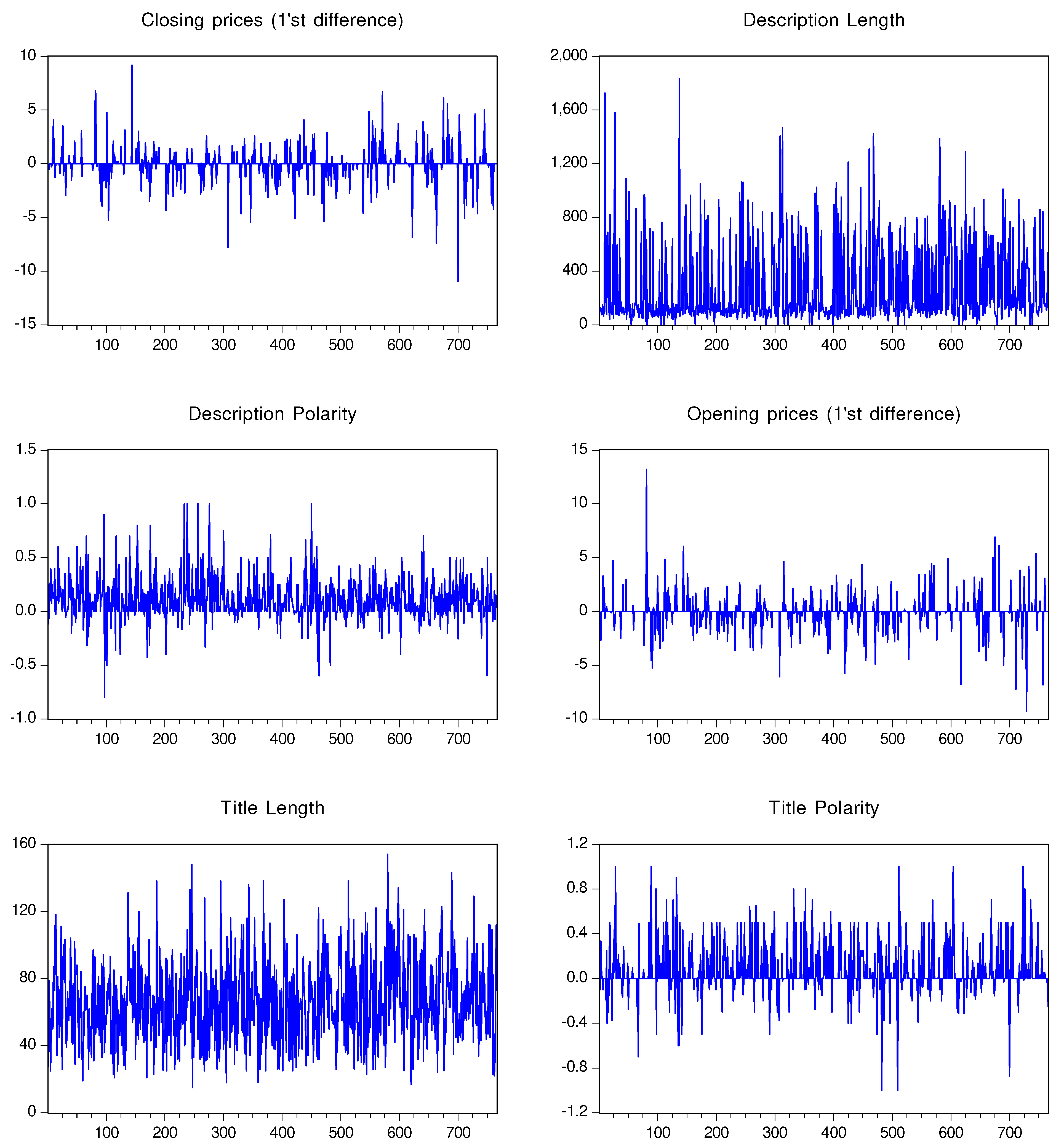
Figure 2.
Microsoft variable graphs
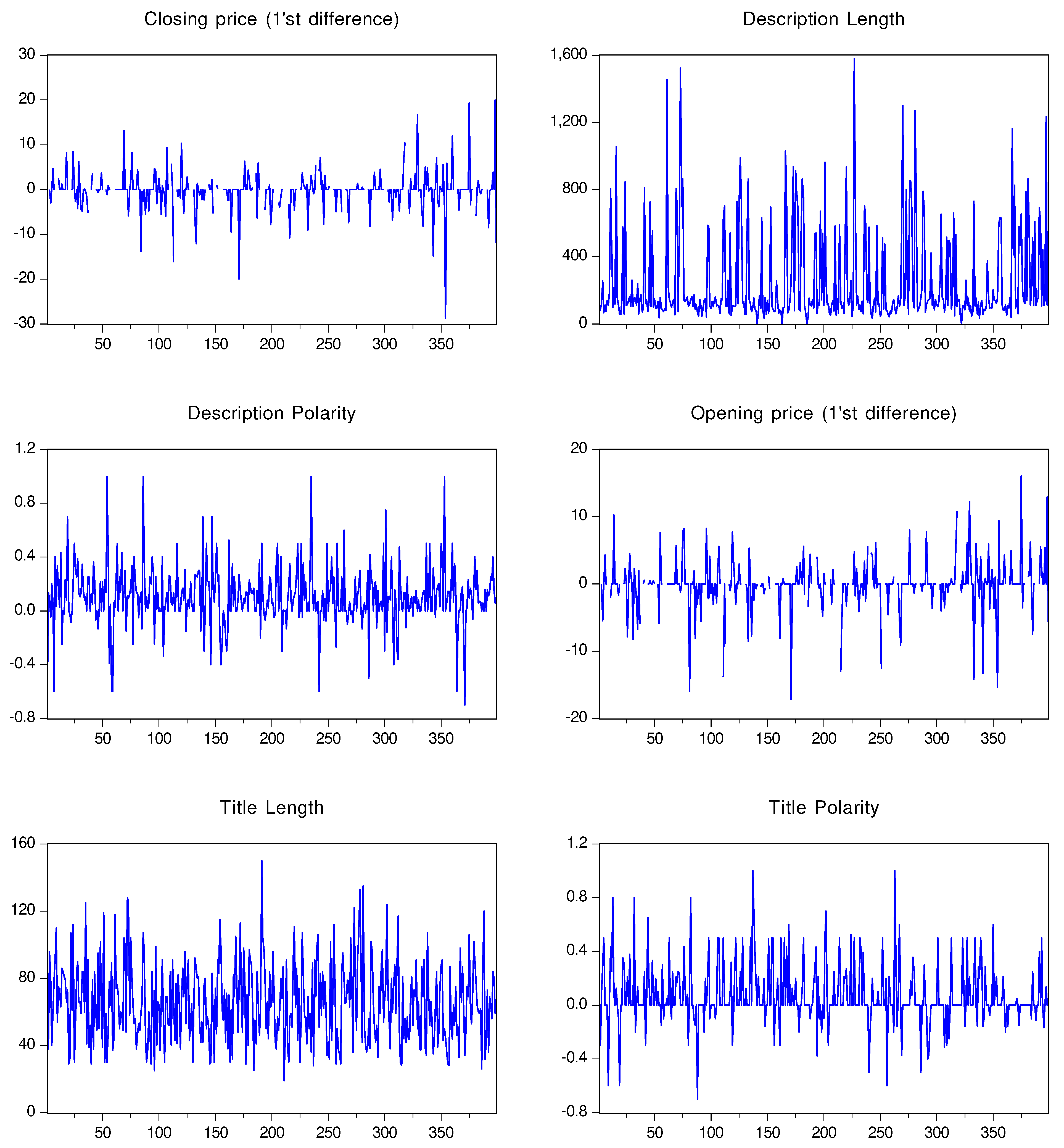
Figure 3.
Tesla variable graphics
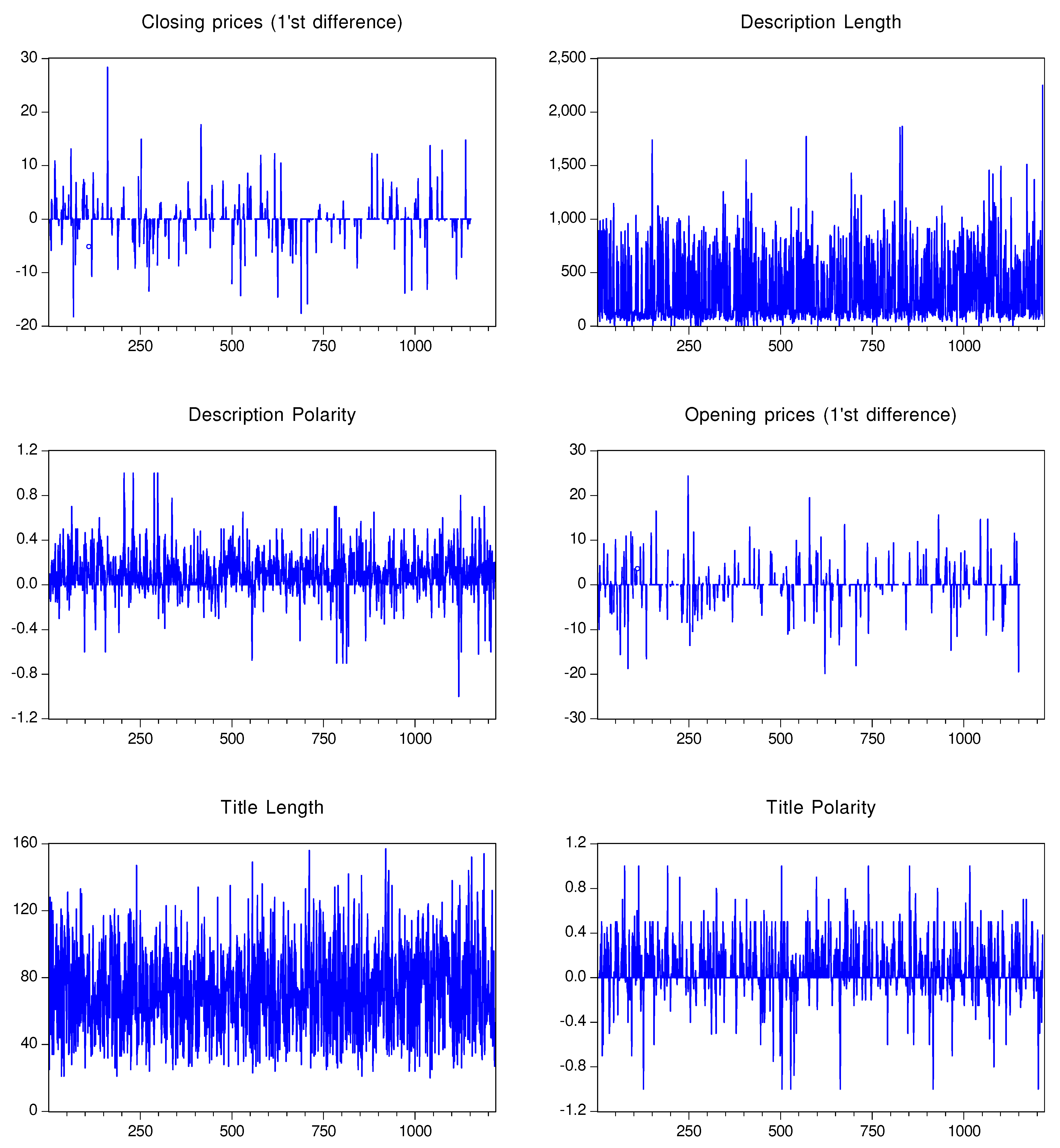
Figure 4.
Wavelet coherence of Apple stock title polarity (A) and closing prices (B).
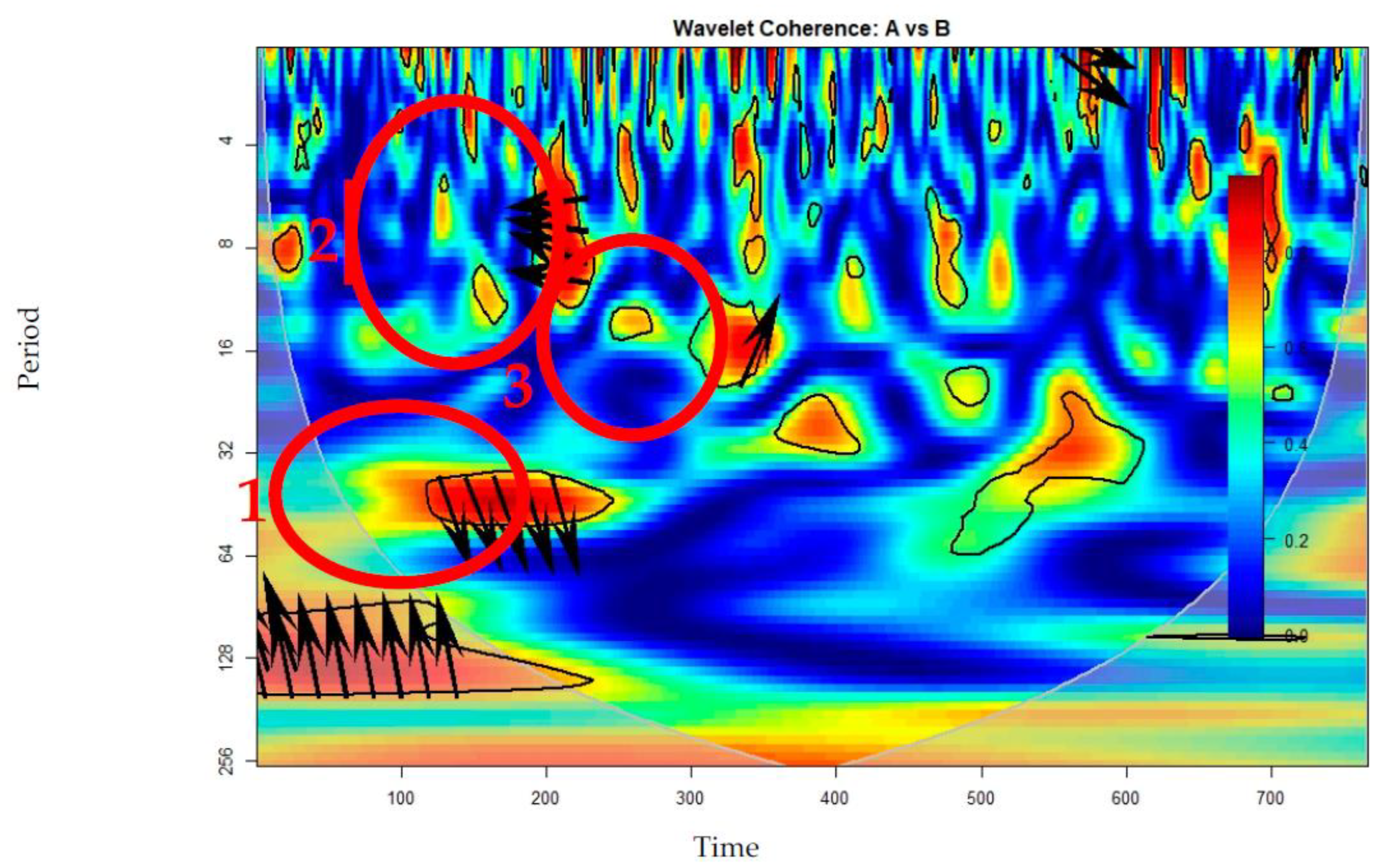
Figure 5.
Wavelet coherence of Microsoft stock description polarity (A) and opening prices (B).
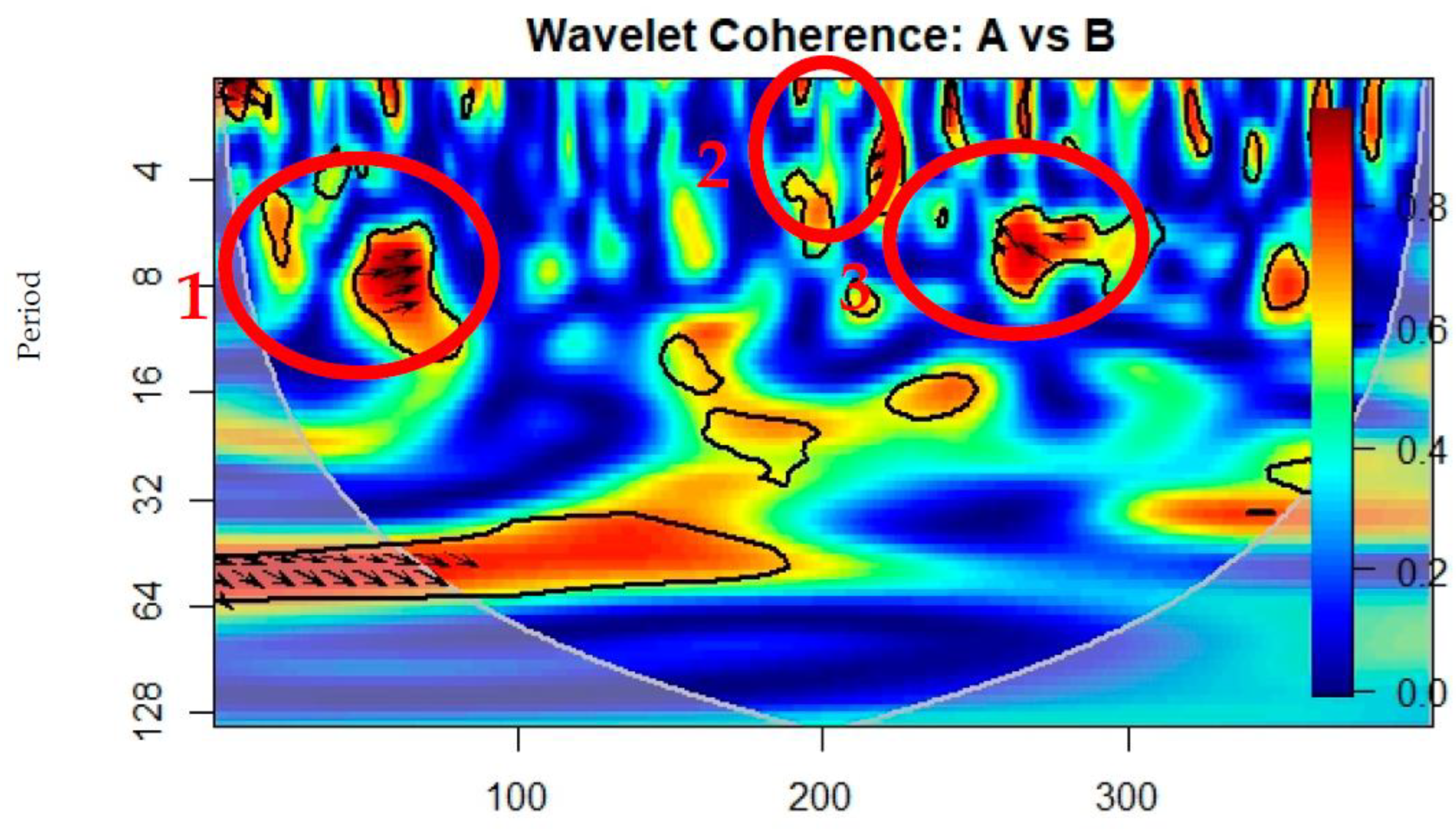
Figure 6.
Wavelet coherence of Tesla stock title polarity (A) and opening prices (B).

Figure 7.
Scatter plot of Apple closing prices and title polarity; linear, quadratic and cubic regressions
Figure 7.
Scatter plot of Apple closing prices and title polarity; linear, quadratic and cubic regressions

Figure 8.
Scatter plot of Microsoft opening prices and description polarity; linear, quadratic and cubic regressions
Figure 8.
Scatter plot of Microsoft opening prices and description polarity; linear, quadratic and cubic regressions
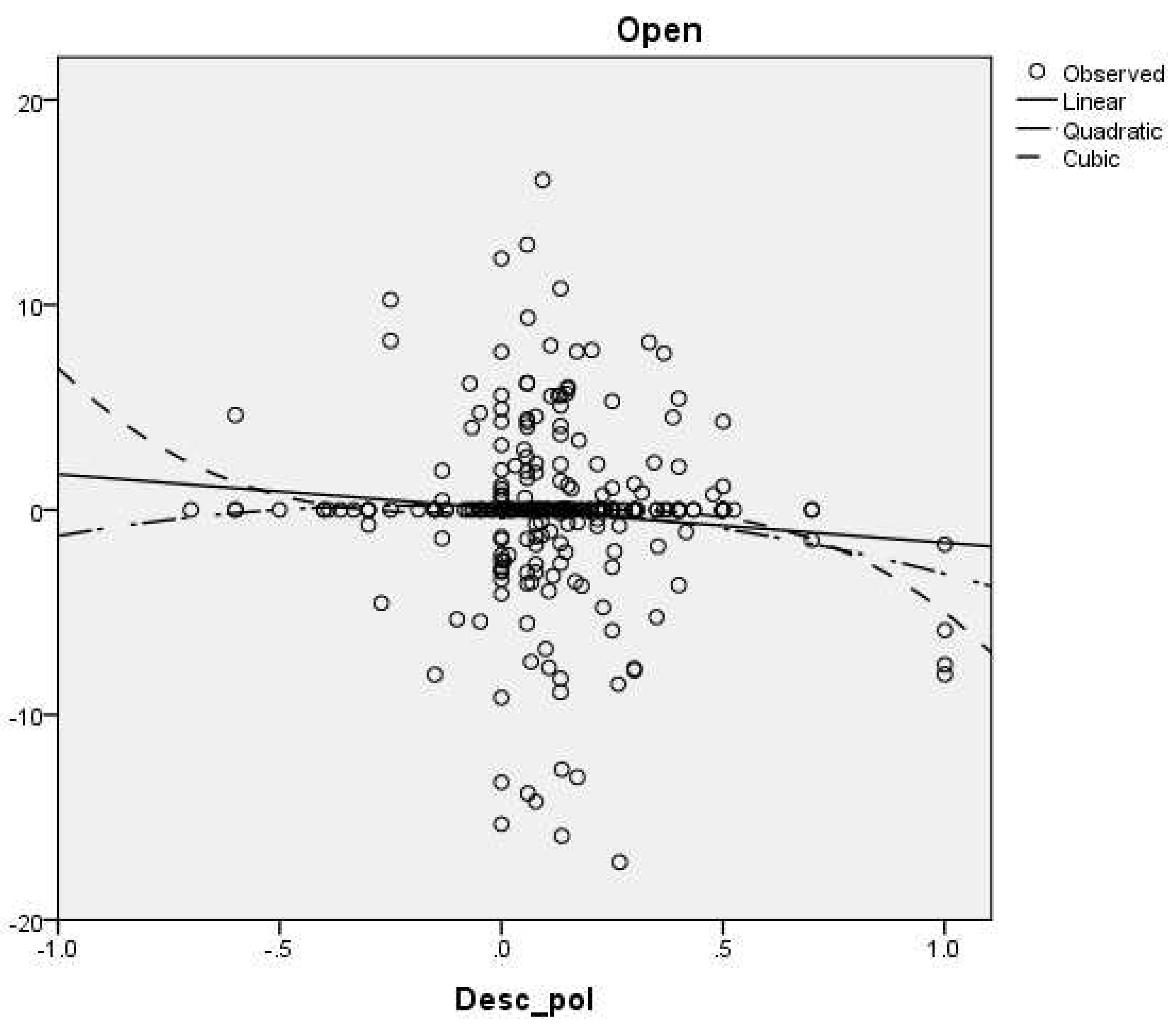
Figure 9.
Scatter plot of Tesla variables: opening prices and title polarity; linear, quadratic and cubic regressions
Figure 9.
Scatter plot of Tesla variables: opening prices and title polarity; linear, quadratic and cubic regressions
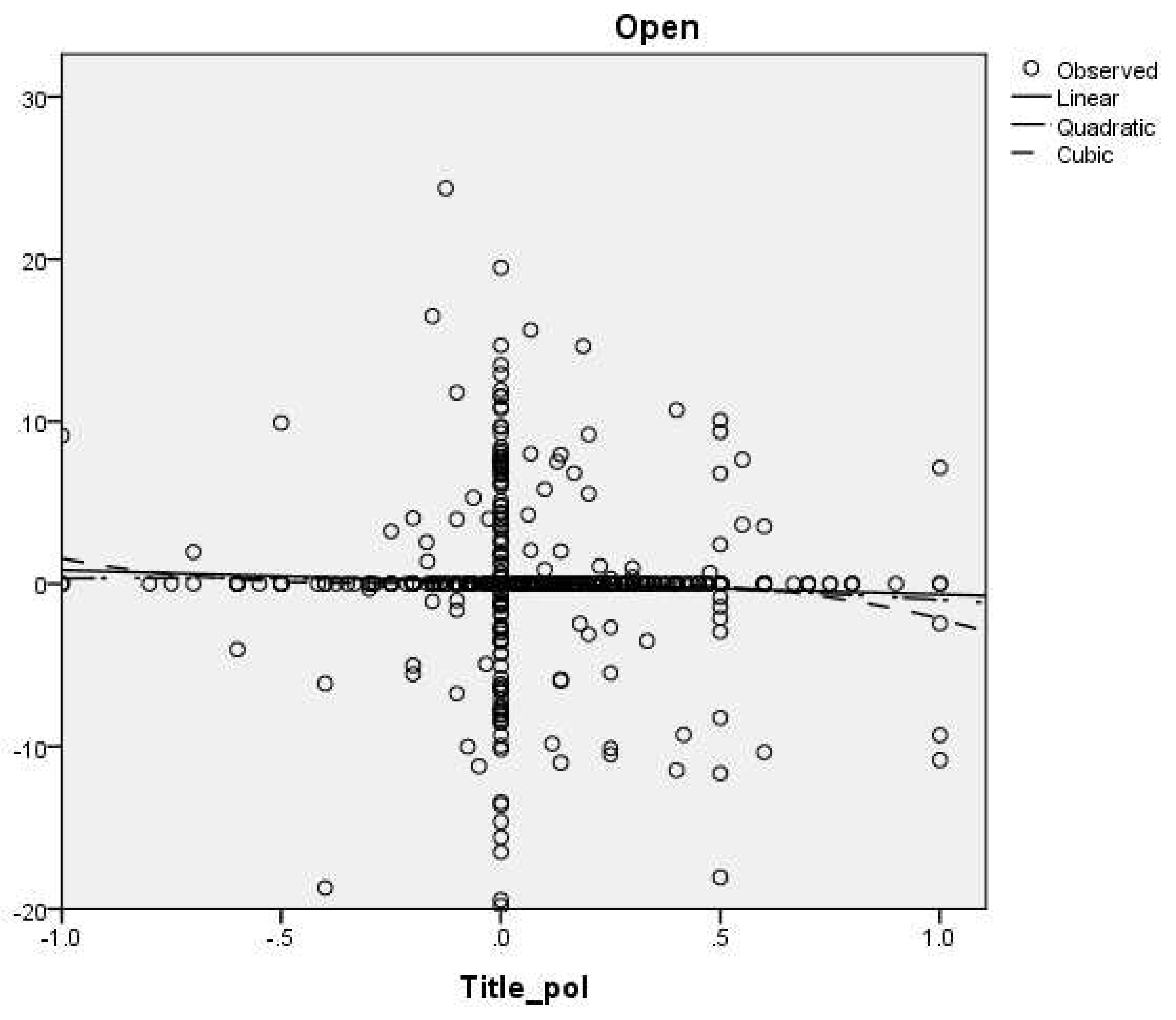
Table 2.
Apple statistics
| CLOSE | DESCRIPTION_LENGTH | DESCRIPTION_POLARITY | OPEN | TITLE_LENGTH | TITLE_POLARITY | |
|---|---|---|---|---|---|---|
| Mean | 160.7906 | 282.9034 | 0.111185 | 160.4305 | 66.15405 | 0.070075 |
| Median | 158.9300 | 135.0000 | 0.075487 | 158.4000 | 63.00000 | 0.000000 |
| Maximum | 196.4500 | 1834.000 | 1.000000 | 196.2400 | 154.0000 | 1.000000 |
| Minimum | 125.0200 | 0.000000 | -0.800000 | 126.0100 | 15.00000 | -1.000000 |
| Std. Dev. | 18.96957 | 304.4415 | 0.200732 | 19.24047 | 25.43293 | 0.230306 |
| Skewness | 0.066746 | 1.576311 | 0.795938 | 0.092734 | 0.474789 | 0.705427 |
| Jarque-Bera | 47.07321 | 485.8930 | 527.9205 | 50.69124 | 29.04518 | 513.8268 |
| Probability | 0.000000 | 0.000000 | 0.000000 | 0.000000 | 0.000000 | 0.000000 |
| Sum | 123165.6 | 216704.0 | 85.16800 | 122889.8 | 50674.00 | 53.67779 |
| Sum Sq. Dev. | 275281.2 | 70903719 | 30.82450 | 283199.8 | 494827.8 | 40.57631 |
| Observations | 766 | 766 | 766 | 766 | 766 | 766 |
Table 3.
Microsoft statistics
| CLOSE | DESCRIPTION_LENGTH | DESCRIPTION_POLARITY | OPEN | TITLE_LENGTH | TITLE_POLARITY | |
|---|---|---|---|---|---|---|
| Mean | 282.3065 | 263.4111 | 0.111952 | 282.2838 | 65.47778 | 0.069444 |
| Median | 275.4200 | 131.0000 | 0.080000 | 278.6100 | 64.00000 | 0.000000 |
| Maximum | 359.4900 | 1581.000 | 1.000000 | 361.7500 | 135.0000 | 1.000000 |
| Minimum | 214.2500 | 0.000000 | -0.700000 | 219.8500 | 25.00000 | -0.700000 |
| Std. Dev. | 42.24372 | 292.9204 | 0.218545 | 42.55378 | 22.95010 | 0.220189 |
| Skewness | 0.179157 | 1.835858 | 0.452213 | 0.186627 | 0.424783 | 0.848019 |
| Jarque-Bera | 35.79734 | 342.3025 | 198.7494 | 36.77976 | 11.81845 | 126.4077 |
| Probability | 0.000000 | 0.000000 | 0.000000 | 0.000000 | 0.002714 | 0.000000 |
| Sum | 101630.4 | 94828.00 | 40.30264 | 101622.2 | 23572.00 | 24.99974 |
| Sum Sq. Dev. | 640646.9 | 30803055 | 17.14655 | 650086.0 | 189087.8 | 17.40554 |
| Observations | 360 | 360 | 360 | 360 | 360 | 360 |
Table 4.
Tesla statistics
| DESCRIPTION_LENGTH | DESCRIPTION_POLARITY | OPEN | CLOSE | TITLE_LENGTH | TITLE_POLARITY | |
|---|---|---|---|---|---|---|
| Mean | 355.3691 | 0.094744 | 194.2592 | 193.8915 | 72.22990 | 0.064005 |
| Median | 155.0000 | 0.066833 | 190.5200 | 190.7200 | 72.00000 | 0.000000 |
| Maximum | 1866.000 | 1.000000 | 296.0400 | 293.3400 | 157.0000 | 1.000000 |
| Minimum | 0.000000 | -1.000000 | 103.0000 | 108.1000 | 20.00000 | -1.000000 |
| Std. Dev. | 336.3253 | 0.191292 | 47.18739 | 46.80205 | 26.71722 | 0.229029 |
| Skewness | 1.074216 | 0.230695 | 0.178609 | 0.146580 | 0.253157 | 0.361534 |
| Jarque-Bera | 197.2607 | 920.0446 | 21.17389 | 20.83806 | 20.06870 | 825.3827 |
| Probability | 0.000000 | 0.000000 | 0.000025 | 0.000030 | 0.000044 | 0.000000 |
| Sum | 344708.0 | 91.90212 | 188431.4 | 188074.7 | 70063.00 | 62.08466 |
| Sum Sq. Dev. | 1.10E+08 | 35.45826 | 2157624. | 2122529. | 691681.7 | 50.82828 |
| Observations | 970 | 970 | 970 | 970 | 970 | 970 |
Table 5.
Apple Dickey Fuller test results
| Variable tested | Augmented Dickey-Fuller test statistic | p-value | level |
|---|---|---|---|
| Closing prices | -27.22329 | 0.000 | 1’st difference |
| Description length | -26.23105 | 0.000 | No difference |
| Description polarity | -29.44872 | 0.000 | No difference |
| Opening prices | -28.13567 | 0.000 | 1’st difference |
| Title length | -26.09943 | 0.000 | No difference |
| Title polarity | -26.84126 | 0.000 | No difference |
Table 6.
Microsoft Dickey Fuller test results
| Variable tested | Augmented Dickey-Fuller test statistic | p-value | level |
|---|---|---|---|
| Description length | -16.50101 | 0.000 | No difference |
| Closing prices | -17.70365 | 0.000 | 1’st difference |
| Description polarity | -20.73954 | 0.000 | No difference |
| Opening prices | -17.36869 | 0.000 | 1’st difference |
| Title length | -18.70511 | 0.000 | No difference |
| Title polarity | -18.42411 | 0.000 | No difference |
Table 7.
Tesla Dickey Fuller test results
| Variable tested | Augmented Dickey-Fuller test statistic | p-value | level |
|---|---|---|---|
| Description length | -35.15816 | 0.000 | No difference |
| Closing prices | -28.99028 | 0.000 | 1’st difference |
| Description polarity | -34.20196 | 0.000 | No difference |
| Opening prices | -29.56049 | 0.000 | 1’st difference |
| Title length | -35.74526 | 0.000 | No difference |
| Title polarity | -35.04870 | 0.000 | No difference |
Table 8.
Apple variables Pearson correlation
| Variable: -Pearson Correl. -Sig. -N |
Open | Close |
|---|---|---|
| Title Polarity | -.034 | .080* |
| .345 | .027 | |
| 765 | 765 | |
| Title Length | -.001 | .065 |
| .976 | .073 | |
| 765 | 765 | |
| Description Polarity | -.024 | .014 |
| .511 | .709 | |
| 765 | 765 | |
| Description Length | .018 | .052 |
| .612 | .149 | |
| 765 | 765 | |
| *. Correlation is significant at the 0.05 level (2-tailed). | ||
| **. Correlation is significant at the 0.01 level (2-tailed). | ||
Table 9.
Microsoft variables Pearson correlation
| Variable: -Pearson Correl. -Sig. -N |
Open | Close |
|---|---|---|
| Title Polarity | .012 | .030 |
| .833 | .583 | |
| 333 | 333 | |
| Title Length | .077 | .061 |
| .161 | .268 | |
| 333 | 333 | |
| Description Polarity | -.095 | -.041 |
| .085 | .457 | |
| 333 | 333 | |
| Description Length | .039 | .037 |
| .476 | .500 | |
| 333 | 333 | |
| *. Correlation is significant at the 0.05 level (2-tailed). | ||
| **. Correlation is significant at the 0.01 level (2-tailed). | ||
Table 10.
Tesla variables Pearson correlation
| Variable: -Pearson Correl. -Sig. -N |
Open | Close |
|---|---|---|
| Title Polarity | -.050 | -.034 |
| .093 | .304 | |
| 920 | 920 | |
| Title Length | .035 | .027 |
| .289 | .417 | |
| 920 | 920 | |
| Description Polarity | -.019 | -.007 |
| .563 | .826 | |
| 920 | 920 | |
| Description Length | -.015 | .006 |
| .653 | .859 | |
| 920 | 920 | |
| **. Correlation is significant at the 0.01 level (2-tailed). | ||
Table 11.
Glejser heteroskedasticity test for Apple title polarity and closing prices linear regressions residuals
Table 11.
Glejser heteroskedasticity test for Apple title polarity and closing prices linear regressions residuals
| Heteroskedasticity Test: Glejser | ||||
| F-statistic | 1.813126 | Prob. F(1,763) | 0.1785 | |
| Obs*R-squared | 1.813569 | Prob. Chi-Square(1) | 0.1781 | |
| Scaled explained SS | 3.896071 | Prob. Chi-Square(1) | 0.0484 | |
| Test Equation: | ||||
| Dependent Variable: ARESID | ||||
| Method: Least Squares | ||||
| Date: 10/17/23 Time: 10:36 | ||||
| Sample: 2 766 | ||||
| Included observations: 765 | ||||
| Variable | Coefficient | Std. Error | t-Statistic | Prob. |
| C | 0.700303 | 0.048864 | 14.33181 | 0.0000 |
| TITLE_POLARITY | -0.273302 | 0.202968 | -1.346524 | 0.1785 |
| R-squared | 0.002371 | Mean dependent var | 0.681126 | |
| Adjusted R-squared | 0.001063 | S.D. dependent var | 1.293509 | |
| S.E. of regression | 1.292821 | Akaike info criterion | 3.354141 | |
| Sum squared resid | 1275.268 | Schwarz criterion | 3.366272 | |
| Log likelihood | -1280.959 | Hannan-Quinn criter. | 3.358811 | |
| F-statistic | 1.813126 | Durbin-Watson stat | 2.180885 | |
| Prob(F-statistic) | 0.178534 | |||
Table 12.
Glejser heteroskedasticity test for Microsoft description polarity and opening prices linear regressions residuals
Table 12.
Glejser heteroskedasticity test for Microsoft description polarity and opening prices linear regressions residuals
| Heteroskedasticity Test: Glejser | ||||
| F-statistic | 0.598667 | Prob. F(1,331) | 0.4396 | |
| Obs*R-squared | 0.601196 | Prob. Chi-Square(1) | 0.4381 | |
| Scaled explained SS | 1.161268 | Prob. Chi-Square(1) | 0.2812 | |
| Test Equation: | ||||
| Dependent Variable: ARESID | ||||
| Method: Least Squares | ||||
| Date: 10/17/23 Time: 10:44 | ||||
| Sample: 3 399 | ||||
| Included observations: 333 | ||||
| Variable | Coefficient | Std. Error | t-Statistic | Prob. |
| C | 2.026960 | 0.199382 | 10.16620 | 0.0000 |
| DESCRIPTION_POLARITY | 0.627657 | 0.811204 | 0.773735 | 0.4396 |
| R-squared | 0.001805 | Mean dependent var | 2.095826 | |
| Adjusted R-squared | -0.001210 | S.D. dependent var | 3.253779 | |
| S.E. of regression | 3.255747 | Akaike info criterion | 5.204708 | |
| Sum squared resid | 3508.563 | Schwarz criterion | 5.227580 | |
| Log likelihood | -864.5840 | Hannan-Quinn criter. | 5.213829 | |
| F-statistic | 0.598667 | Durbin-Watson stat | 1.983603 | |
| Prob(F-statistic) | 0.439640 | |||
Table 13.
Glejser heteroskedasticity test for Tesla title polarity and opening prices linear regressions residuals
Table 13.
Glejser heteroskedasticity test for Tesla title polarity and opening prices linear regressions residuals
| Heteroskedasticity Test: Glejser | ||||
| F-statistic | 0.036500 | Prob. F(1,918) | 0.8485 | |
| Obs*R-squared | 0.036578 | Prob. Chi-Square(1) | 0.8483 | |
| Scaled explained SS | 0.085498 | Prob. Chi-Square(1) | 0.7700 | |
| Test Equation: | ||||
| Dependent Variable: ARESID | ||||
| Method: Least Squares | ||||
| Date: 10/17/23 Time: 10:45 | ||||
| Sample: 4 1153 | ||||
| Included observations: 920 | ||||
| Variable | Coefficient | Std. Error | t-Statistic | Prob. |
| C | 1.338588 | 0.110216 | 12.14512 | 0.0000 |
| TITLE_POLARITY | 0.087392 | 0.457429 | 0.191050 | 0.8485 |
| R-squared | 0.000040 | Mean dependent var | 1.344273 | |
| Adjusted R-squared | -0.001050 | S.D. dependent var | 3.217169 | |
| S.E. of regression | 3.218857 | Akaike info criterion | 5.178101 | |
| Sum squared resid | 9511.435 | Schwarz criterion | 5.188589 | |
| Log likelihood | -2379.927 | Hannan-Quinn criter. | 5.182103 | |
| F-statistic | 0.036500 | Durbin-Watson stat | 2.253205 | |
| Prob(F-statistic) | 0.848529 | |||
Table 14.
Regressions results for Apple variables: closing prices and title polarity
| Model Summary and Parameter Estimates | |||||||||
|---|---|---|---|---|---|---|---|---|---|
| Dependent Variable: Close (Closing prices) | |||||||||
| Equation | Model Summary | Parameter Estimates | |||||||
| R Square | F | df1 | df2 | Sig. | Constant | b1 | b2 | b3 | |
| Linear | .006 | 4.942 | 1 | 764 | .027 | -.079 | .510 | ||
| Quadratic | .012 | 4.478 | 2 | 763 | .012 | -.047 | .773 | -.868 | |
| Cubic | .013 | 3.446 | 3 | 762 | .016 | -.036 | .466 | -.978 | .836 |
| The independent variable is Title polarity. | |||||||||
Table 15.
Parameter estimation of the autoregression with exogenous factor, for the Apple closing prices and title polarity
Table 15.
Parameter estimation of the autoregression with exogenous factor, for the Apple closing prices and title polarity
| Parameter Estimates | ||||
|---|---|---|---|---|
| Parameter | Estimate | Std. Error | 95% Confidence Interval | |
| Lower Bound | Upper Bound | |||
| .014 | .036 | -.057 | .085 | |
| .414 | .220 | -.018 | .846 | |
Table 16.
Goodness of fit for the autoregression with exogenous factor, for the Apple closing prices and title polarity
Table 16.
Goodness of fit for the autoregression with exogenous factor, for the Apple closing prices and title polarity
| ANOVAa | |||
|---|---|---|---|
| Source | Sum of Squares | df | Mean Squares |
| Regression | 7.944 | 2 | 3.972 |
| Residual | 1637.255 | 763 | 2.146 |
| Uncorrected Total | 1645.199 | 765 | |
| Corrected Total | 1643.774 | 764 | |
| Dependent variable: Close | |||
| a. R squared = 1 - (Residual Sum of Squares) / (Corrected Sum of Squares) = .004. | |||
Table 17.
Regressions results for Microsoft variables: opening prices and description polarity
| Model Summary and Parameter Estimates | |||||||||
|---|---|---|---|---|---|---|---|---|---|
| Dependent Variable: Open | |||||||||
| Equation | Model Summary | Parameter Estimates | |||||||
| R Square | F | df1 | df2 | Sig. | Constant | b1 | b2 | b3 | |
| Linear | .009 | 2.983 | 1 | 331 | .085 | .061 | -1.669 | ||
| Quadratic | .014 | 2.260 | 2 | 330 | .106 | .119 | -.924 | -2.319 | |
| Cubic | .023 | 2.606 | 3 | 329 | .052 | -.104 | .561 | 1.067 | -6.530 |
| The independent variable is Description_polarity. | |||||||||
Table 18.
Regressions results for Tesla variables: opening prices and title polarity
| Model Summary and Parameter Estimates | |||||||||
| Dependent Variable: Open | |||||||||
| Equation | Model Summary | Parameter Estimates | |||||||
| R Square | F | df1 | df2 | Sig. | Constant | b1 | b2 | b3 | |
| Linear | .002 | 2.290 | 1 | 919 | .131 | .086 | -.750 | ||
| Quadratic | .003 | 1.274 | 2 | 918 | .280 | .105 | -.654 | -.439 | |
| Cubic | .005 | 1.499 | 3 | 917 | .213 | .078 | .208 | -.374 | -2.070 |
| The independent variable is Title_polarity. | |||||||||
Table 19.
Parameter estimation of the autoregression with exogenous factor, for the Tesla opening prices and title polarity
Table 19.
Parameter estimation of the autoregression with exogenous factor, for the Tesla opening prices and title polarity
| Parameter Estimates | ||||
|---|---|---|---|---|
| Parameter | Estimate | Std. Error | 95% Confidence Interval | |
| Lower Bound | Upper Bound | |||
| .902 | .029 | .846 | .959 | |
| .038 | .029 | -.018 | .094 | |
| 16.999 | 7.182 | 2.909 | 31.089 | |
Table 20.
Goodness of fit for the autoregression with exogenous factor, for the Tesla opening prices and title polarity
Table 20.
Goodness of fit for the autoregression with exogenous factor, for the Tesla opening prices and title polarity
| ANOVAa | |||
|---|---|---|---|
| Source | Sum of Squares | df | Mean Squares |
| Regression | 34496314.240 | 3 | 11498771.413 |
| Residual | 4265830.600 | 1214 | 3513.864 |
| Uncorrected Total | 38762144.839 | 1217 | |
| Corrected Total | 9586807.822 | 1216 | |
| Dependent variable: Open | |||
| R squared = 1 - (Residual Sum of Squares) / (Corrected Sum of Squares) = .555. | |||
Disclaimer/Publisher’s Note: The statements, opinions and data contained in all publications are solely those of the individual author(s) and contributor(s) and not of MDPI and/or the editor(s). MDPI and/or the editor(s) disclaim responsibility for any injury to people or property resulting from any ideas, methods, instructions or products referred to in the content. |
© 2023 by the authors. Licensee MDPI, Basel, Switzerland. This article is an open access article distributed under the terms and conditions of the Creative Commons Attribution (CC BY) license (http://creativecommons.org/licenses/by/4.0/).
Copyright: This open access article is published under a Creative Commons CC BY 4.0 license, which permit the free download, distribution, and reuse, provided that the author and preprint are cited in any reuse.


