Preprint
Article

Intelligent Feedrate Optimization using an Uncertainty-aware Digital Twin within a Model Predictive Control Framework

Altmetrics

Downloads

228

Views

144

Comments

1

A peer-reviewed article of this preprint also exists.

This version is not peer-reviewed

Submitted:

02 November 2023

Posted:

03 November 2023

Read the latest preprint version here

Alerts
Abstract
The future of intelligent manufacturing machines involves autonomous selection of process parameters to maximize productivity while maintaining quality within specified constraints. To effectively optimize process parameters, these machines need to adapt to existing uncertainties in the physical system. This paper proposes a novel framework and methodology for feedrate optimization that is based on a physics-informed data-driven digital twin with quantified uncertainty. The servo dynamics are modeled using a digital twin, which incorporates the known uncertainty in the physics-based models and predicts the distribution of contour error using a data-driven model that learns the unknown uncertainty on-the-fly by sensor measurements. Using the quantified uncertainty, the proposed feedrate optimization maximizes productivity while maintaining quality under desired servo error constraints and stringency (i.e., the tolerance for constraint violation under uncertainty) using a model predictive control framework. Experimental results obtained using a 3-axis desktop CNC machine tool and a desktop 3D printer demonstrate significant cycle time reductions of up to 38% and 17% respectively, while staying close to the error tolerances compared to the existing methods.
Keywords: 
Subject: Engineering  -   Industrial and Manufacturing Engineering

1. Introduction

Quality and productivity are two important and frequently competing factors in manufacturing. As a result, manufacturers strive to maximize productivity while adhering to quality constraints. In practice, achieving this goal has involved a trial-and-error approach. However, there is a growing demand for self-optimizing intelligent manufacturing machines that have the capability to autonomously optimize their speed while ensuring desired quality levels, eliminating the need for extensive trial-and-error [1].
Motion-induced servo error, which is one of the major sources of quality degradation in manufacturing machines, can result from the limited bandwidth of feedback controllers, flexible structures, nonlinear friction, and backlash. Another source of servo error is process force, such as cutting force. Given that motion- and process-force-induced servo errors tend to increase with higher speeds, there is a keen interest in maximizing the speed of motion while respecting the tolerances on motion- and/or process-induced servo errors.
Extensive research has been conducted in the field of feedrate optimization with the objective of maximizing the feedrate while respecting servo error constraints. The majority of feedrate optimization or feedrate scheduling techniques primarily focus on maximizing the feedrate while considering kinematic limits such as speed, acceleration, and jerk [2,3,4,5,6,7]. However, the existing studies in [2,3,4,5,6,7] do not incorporate dynamic constraints such as servo error and cutting force, resulting in the need for a cautious selection of kinematic limits to indirectly meet the requirements on dynamic constraints. This indirect approach is necessary due to the complex relationship between kinematics and dynamic constraints, which often leads to sub-optimal feedrates.
In order to directly enforce dynamic constraints, certain feedrate optimization methods incorporate limits on the servo error, in addition to kinematics, by using steady-state [8] or static [9,10] approximations of servo models associated with motion velocity and acceleration. However, their limited ability to directly incorporate dynamic aspects of servo error, such as dynamic servo error pre-compensation, hinders their accuracy and effectiveness in optimizing feedrate.
To directly incorporate dynamic components via physics-based models, numerous feedrate scheduling methods for CNC machines maximize feedrate in each NC block while keeping cutting force under desired levels via mechanistic force models [11,12,13,14,15,16,17,18]. Some feedrate scheduling techniques maximize feedrate while regulating machining error due to tool deflection [19,20,21,22,23,24,25] or force-induced servo error [26,27] under desired tolerance in CNC machine tools. A few works in feedrate optimization [28,29] constrain motion-induced error via linear physics-based models of servo dynamics. However, the works in [11,12,13,14,15,16,17,18,19,20,21,22,23,24,25,26,27,28,29] are unable to effectively constrain actual cutting force or servo error in situations where uncertainties arise from nonlinear dynamics or disturbances that are not incorporated in the physics-based models. As a result, their capability to maximize feedrate while adhering to dynamic constraints is severely restricted.
There is increasing interest in the utilization of digital twins in manufacturing. A digital twin is a virtual representation, parallel to a physical system, built on a bi-directional link between simulation and actual data collection [1]. To effectively optimize feedrate with existence of uncertainties, digital twins can be used to provide more-accurate predictions of process or servo dynamics for feedrate optimization using data-driven models updated via sensor measurements. Model predictive control (MPC) is a framework often used for optimizing feedrate using digital twins. In MPC [30], predictions made using physics-based and data acquired from sensors are used to optimize an objective in a receding horizon fashion. In the context of feedrate optimization, a linear hybrid model was augmented with a periodic internal model in a MPC framework [31] to effectively predict and constrain servo errors due to motion and cutting forces. Luenberger state observers [32] were used in feedrate optimization to correct the initial system states of servo dynamic models in real-time for accurate contour error constraint enforcement, where the objective function was based on a tunable index of how far away an unattainable target position is from the current position. Similarly, a two-stage MPC approach was proposed in [33], where the first stage performed feedrate optimization with contour error constraints using a linear data-driven model, and the second stage further pre-compensated the contour error using artificial neural networks (ANNs). However, the data-driven models in [33] were trained offline through numerous experiments, which is time-consuming and may not be effective in predicting contour error in the presence of in-situ uncertainties that are not included in the training data. Moreover, the two-stage optimizations in [33] and the mixed objective functions used to balance quality and productivity in [32,33] require trial-and-error to tune the objective function weights to determine an acceptable quality level. Therefore, it is better to enforce quality requirements as contour error constraints that must be met, as is often the case in practice. Furthermore, the existing MPC methods in [31,32,33] do not quantify or exploit the uncertainty of the prediction in their feedrate optimization. Hence, they may not effectively adhere to constraints in the presence of high uncertainty due to a lack of training data, system variability and sudden changes in operating conditions.
To quantify uncertainties and impose robustness, studies exist on maximizing feedrate while regulating spindle power, where the spindle power is modeled using Gaussian process regression (GPR) [34]. The spindle power constraint is derived from a stochastic constraint with a fixed confidence level to safely optimize feedrate in uncertain environments. However, GPR in [34] is updated cycle-by-cycle, where the first cycle is initialized with a conservative feedrate profile followed by numerous sequential cycles for convergence. This requires optimizing a highly non-linear GPR objective [35] to estimate hyperparameters, which renders the process less adaptable to real-time control. Moreover, it does not constrain the servo error nor account for the propagation of model uncertainties to the servo error. This oversight is critical in achieving desired part accuracy in feedrate optimization, especially for toolpaths with high curvatures that can create significant structural vibration.
To address the shortcomings of the existing works, this paper proposes an intelligent feedrate optimization with contour error constraints using an uncertainty-aware digital twin, by making the following original contributions:
  • It uses a novel physics-informed data-driven digital twin to predict the contour error and its uncertainty, where the digital twin incorporates the known uncertainty in the physics-based models and learns the unknown uncertainty by correcting the data-driven model on-the-fly using sensor feedback.
  • It formulates an intelligent feedrate optimization framework capable of maximizing feedrate while accurately constraining contour error under desired tolerance and stringency, based on the uncertainty estimation from the digital twin using a model predictive control framework.
  • It demonstrates the effectiveness of the proposed method by validating its performance in simulations and experiments using a desktop CNC machine tool and 3D printer.
The outline of the paper is as follows: Section 2 introduces our framework for intelligent feedrate optimization using an uncertainty-aware digital twin. Section 3 describes the methodology of the proposed digital twin for predicting the contour error distribution. Section 4 provides a formulation of the feedrate optimization with contour error and stringency constraints (i.e., the tolerance for constraint violation under uncertainty). Section 5 numerically validates the proposed method via a desktop CNC machine tol. Section 6 experimentally validates the proposed method via a desktop CNC machine tool and 3D printer. Finally, Section 7 concludes the paper and discusses future work.

2. Framework for Feedrate Optimization with Uncertainty-aware Digital Twin

The framework for the proposed intelligent feedrate optimization with an uncertainty-aware digital twin is depicted in Figure 1. First, a manufacturer submits a part together with the desired dimensions and contour error tolerance to an intelligent manufacturing machine. Then, the goal of the machine is to autonomously produce the part as quickly as possible while respecting the given error tolerance. The machine is equipped with a digital twin that predicts the contour error, which the machine can exploit for feedrate optimization with contour error constraints. Hence, the proposed framework is based on model predictive control.
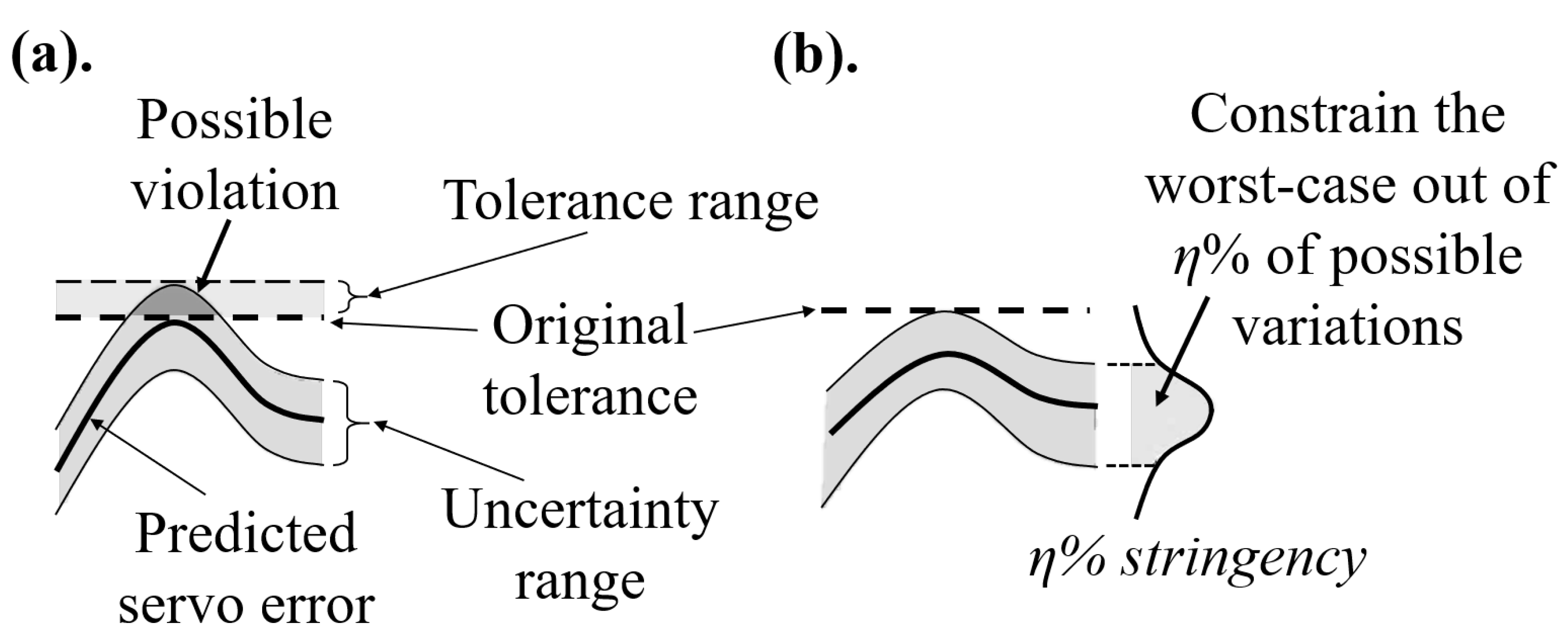
However, several uncertainties exist in the physical system. Some portions are known from available data or expert knowledge, while others, such as nonlinear dynamics, may be unknown. If not considered, the known and unknown uncertainties cause a violation in the contour error tolerance, hence the part quality, as illustrated in Figure 2(a).
However, given that uncertainty exists in enforcing tolerance constraints, manufacturers have different levels of stringency in enforcing constraints. For example, a manufacturer may want at least 99% of the produced parts to satisfy the constraints. Therefore, stringency reflects a manufacturer’s tolerance for quality constraint violations under uncertainty. In this paper, we propose that, instead of relying on trial-and-error, manufacturers can impose a desired stringency η % on the given tolerance by incorporating the uncertainty of the contour error prediction as shown in Figure 2(b). Imposing the stringency represents constraining the worst case out of η % of the entire variation of contour error, so that η % of the manufactured parts adhere to the imposed kinematic and tolerance constraints under the given uncertainty.
To do so, the digital twin uses the known uncertainty from the physics-based models and trains a data-driven model using the machine’s sensor measurements to learn the unknown uncertainty. The digital twin then predicts and quantifies the uncertainty of the contour error, which is used in feedrate optimization with desired tolerance and stringency on the contour error. Together with the uncertainty-aware digital twin, the feedrate optimization determines the fastest feedrate to run the machine while respecting the limits for the contour errors (and the kinematic limits of the machine) in a robust way. The measured sensor output is compared with the predicted output and used to adjust the digital twin and optimization algorithm in the next iteration of feedrate optimization.
Figure 2. (a) Need for a tolerance range due to violation of error tolerance in the presence of uncertainties, (b) Proposed method of feedrate optimization with desired tolerance stringency using quantified uncertainty.
Preprints 89465 g002

3. Contour error prediction with a real-time uncertainty-aware digital twin

This section first describes the methodology of the contour error prediction using a deterministic digital twin in Section 3.1, and extends it to prediction of contour error and its distribution using an uncertainty-aware digital twin in Section 3.2.

3.1. Overview of contour error prediction using a deterministic digital twin

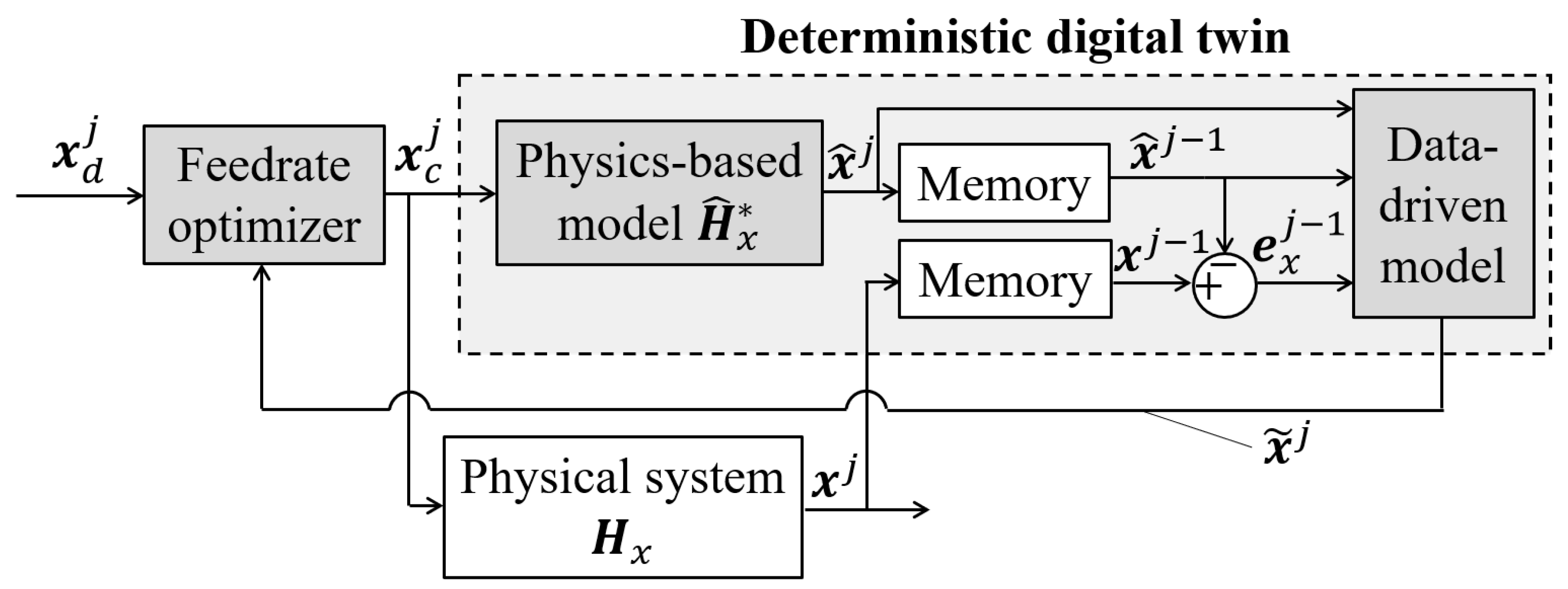
A flowchart of the intelligent feedrate optimization using a deterministic digital twin based on the previous work in [31] is depicted in Figure 3. Note that the internal model in [31] is removed. Also note that Figure 3, as well as the discussions that follow in this section, focus on only the x-axis for the sake of brevity. However, the exact same process can be applied to the y-axis and other independent axes of a Cartesian configured manufacturing machine. Small batches (i.e., look-ahead windows) x d j of a desired position trajectory x d are fed into an intelligent feedrate optimizer to produce the optimized motion command, x c j , where the superscript j { 0 , 1 , 2 , } represents the batch index. Here, each batch has a window length of n w and is defined on the time domain t { 0 , T s , 2 T s , 3 T s , } which represents discrete time at sampling interval T s , as illustrated in Figure 4. The optimized motion commands are sent to the servo system H x to produce the actual position x j . The servo system is composed of a servo error pre-compensation C x followed by machine dynamics G x , i.e., H x = G x C x .
A key requirement for the intelligent feedrate optimization is accurate prediction of the servo error, which is achieved using linear regression built upon the hybrid model presented in [36]. The hybrid model takes input x c j and predicts the actual position x ^ j using a stable, nominal (or representative) physics-based model H ^ x * . The predictions x ^ j do not capture the effects of unmodeled dynamics and external disturbances. Therefore, the prediction error of H ^ x * (delayed by one batch) is computed as e x j 1 = x j 1 x ^ j 1 and combined with x ^ j and x ^ j 1 to be fed into a data driven model to generate an improved prediction x ˜ j which is used for constraining contour errors in the feedrate optimization.
Each element x ˜ ( t ) of x ˜ is modeled as
x ˜ ( t ) = β T ψ t
where ψ t is the deterministic feature vector and β is the weight vector that is learned using linear regression. Note that the superscript j, i.e., batch index, has been removed from x ˜ ( t ) in Eq. (1) to directly define x ˜ in time domain. The sub elements of ψ t are given by
ψ t = [ 1 : = ψ t 1 , x ^ ( t n 2 T s ) , , x ^ ( t ) , : = ψ t 2 e x ( t n 3 T s ) , , e x ( t T s ) ] : = ψ t 3 T
The sub-elements ψ t 1 , ψ t 2 and ψ t 3 were contained in the hybrid model of [36]. They respectively represent a bias term, the past n 2 and current time steps of x ^ , and the past n 3 time steps of e x , where n 2 and n 3 are user defined.
The weight β is updated recursively in each timestep within a given window, where the final weight is carried over to the next window for prediction, i.e., x ˜ j is predicted based on weight β from the previous batch j 1 . The algorithm for learning β is described as follows. For t = 0 , β and its covariance matrix P are initialized using ridge regression with a regularization factor λ as
β = ( λ I + ψ t ψ t T ) 1 ψ t x ( t ) P = ( λ I + ψ t ψ t T ) 1
For the rest of the timesteps t { T s , 2 T s , . . . } , a recursive least-squares is used to correct β and P using a forgetting factor f 0 as
β β + k ( x ( t ) β T ψ t ) P 1 f 0 ( P k ψ t T P ) where   k = P ψ t ( f 0 + ψ t T P ψ t ) 1
Using the final weight in batch j 1 to substitute for β , x ˜ j can be predicted using the feature vector ψ t formulated by Eq. (2). Since the past sensor data x j 1 is provided up to t = ( j n w 1 ) T s , for entries in batch j that have unavailable terms in ψ t 3 , e x for all batches is approximated using the predicted values of x ˜ , i.e.,
e x = x x ^ x ˜ x ^
The same procedure is applied to the y-axis to predict y ˜ . Lastly, the contour error ε ˜ can be estimated from the predicted axis tracking errors ε ˜ x = x d x ˜ and ε ˜ y = y d y ˜ , using a linear approximation [37] as
ε ˜ = sin ( θ ) ε ˜ x + cos ( θ ) ε ˜ y
where θ is inclination angle of the curve ( x d , y d ).

3.2. Prediction and uncertainty quantification of contour error using uncertainty-aware digital twin

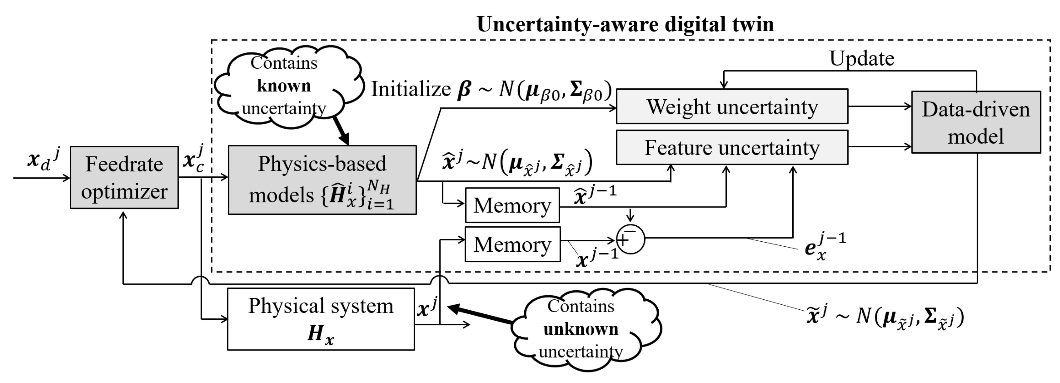
The accuracy of the predictions of the physics-based and data-driven servo models in Section 3.1 can be improved by incorporating the known uncertainty from the physics-based models. To do so, a digital twin that uses physics-informed data-driven servo model is proposed, which is updated on-the-fly via Bayesian approach that is capable of considering uncertainty in the feature vector ψ t . A flowchart of the proposed intelligent feedrate optimization using the uncertainty-aware digital twin is given in Figure 5. The key difference between Figure 3 and Figure 5 is that known uncertainty is included in H ^ x , and unknown uncertainty embedded in x j is learned using the data-driven model and used to predict x ^ j with quantified uncertainty.
Figure 5. Flowchart of intelligent feedrate optimization using an uncertainty-aware digital twin (with physics-based and data-driven servo models, y-axis omitted).
Preprints 89465 g005
Each element x ˜ ( t ) of the digital twin’s prediction of the output position x ˜ j is modeled as
x ˜ ( t ) = β T ψ t + ϵ
where ψ t N ( μ ψ t , Σ ψ t ) is the feature vector defined as an uncorrelated Gaussian random variable with mean μ ψ t and variance Σ ψ t derived from the uncertainty distribution of ψ t previously defined in Eq. (2). β N ( μ β , Σ β ) is the weight vector defined as a correlated Gaussian random variable learned via Bayesian linear regression, and ϵ N ( 0 , σ ϵ 2 ) is the unobserved Gaussian noise. Unlike the deterministic point-estimation of x ˜ j from Section 3.1, a distribution x ˜ j N ( μ x ˜ j , Σ x ˜ j ) is estimated in this section based on the uncertainties of the features and the weights.
This paper proposes that the known uncertainties of the physics-based models are embedded into the feature vector ψ t in Eq. (7) to enable efficient training of β . To do so, a set of N H stable physics-based models { H ^ x i } i = 1 N H is obtained, where each model H ^ x i for i { 1 , 2 , . . . , N H } is identified in the form of the complex-valued frequency response function (FRF) of the physical system H x at discrete frequencies ω k via experiments as
H ^ x i ( ω k ) = a i ( ω k ) + b i ( ω k ) j
where ω k = k Δ ω , of which Δ ω is the increment of frequencies, k { 1 , 2 , . . . , N ω 2 1 } where N ω is the number of discrete negative and positive frequencies at which FRF is identified, and j is the unit imaginary number (which should not be confused with the batch index j used as a superscript elsewhere).
Then, the uncertainty in H ^ x is propagated to the finite impulse response h ^ x as follows. The discrete sets { H ^ x i ( ω k ) } i = 1 N H for each k will introduce discrete sets of their real and imaginary coefficients, namely { a i ( ω k ) } i = 1 N H and { b i ( ω k ) } i = 1 N H . For computational efficiency, it is assumed that { a i ( ω k ) } i = 1 N H and { b i ( ω k ) } i = 1 N H are sampled from Gaussian distributions of a ( ω k ) and b ( ω k ) , of which 99.73%, i.e., the 3-sigma range, lie within the minimum and maximum of the identified discrete sets. Then, a ( ω k ) N ( μ a ( ω k ) , σ a ( ω k ) 2 ) can be approximated as
μ a ( ω k ) = max { a ( ω k ) } + min { a ( ω k ) } 2 σ a ( ω k ) = max { a ( ω k ) } μ a ( ω k ) 3
and b ( ω k ) N ( μ b ( ω k ) , σ b ( ω k ) 2 ) can be approximated using the same procedure as Eq. (9).
Then, the impulse response h ^ x (i.e., h ^ x [ n ] for n { 1 , 2 , . . . , N h } ) of the physics-based model with sampling time T s can be formulated using discrete inverse Fourier transform as
h ^ [ n ] = 1 N ω k = N ω 2 N ω 2 1 ( a ( ω k ) + b ( ω k ) j ) e 2 π j ( n 1 ) ( k 1 ) N ω
where N h = 1 T s Δ ω is the maximum estimable length of the impulse response. Then, due to the linearity of Eq. (10), h ^ [ n ] follows a Gaussian distribution h ^ [ n ] N ( μ h ^ [ n ] , σ h ^ [ n ] 2 ) as
μ h ^ [ n ] = 1 N ω k = 1 N ω ( μ a ( ω k ) + μ b ( ω k ) j ) e 2 π j ( n 1 ) ( k 1 ) N ω σ h ^ [ n ] 2 = 1 N ω k = 1 N ω ( σ a ( ω k ) 2 σ b ( ω k ) 2 ) e 2 π j ( n 1 ) ( k 1 ) N ω
Next, the uncertainty in h ^ [ n ] can be propagated to x ^ ( t ) N ( μ x ^ ( t ) , σ x ^ ( t ) 2 ) as
μ x ^ ( t ) = i = 1 N h μ h ^ [ i ] x d ( t i T s ) σ x ^ ( t ) 2 = i = 1 N h σ h ^ [ i ] 2 x d ( t i T s ) 2
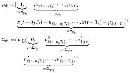
Finally, the feature vector follows an uncorrelated multivariate normal distribution ψ t N ( μ ψ t , Σ ψ t ) , where
Preprints 89465 i001
The prior over β N ( μ β , Σ β ) is initialized using the nominal physics-based model μ h ^ x from Eq. (11), as described in Appendix A. Now given β N ( μ β , Σ β ) and the feature uncertainty ψ t N ( μ ψ t , Σ ψ t ) from Eq. (13), we propose to take a Bayesian route to obtain the posterior over β as more data is collected in real time.
Mathematically, the posterior is given as:
p ( β | x ( t ) , μ ψ t , Σ ψ t ) p ( x ( t ) | β , μ ψ t , Σ ψ t ) · p ( β ) p ( x ( t ) , ψ t | β , μ ψ t , Σ ψ t ) d ψ t · p ( β ) p ( x ( t ) | ψ t , β ) p ( ψ t | μ ψ t , Σ ψ t ) d ψ t · p ( β ) p ( x ( t ) | β ) · p ( β )
where x ( t ) is the actual position on the x-axis at timestep t defined in Section 3.1. Here, p ( x ( t ) | β ) and p ( β ) are given as as
p ( x ( t ) | β ) = exp ( 1 2 ( x ( t ) β T μ ψ t ) T ( β T Σ ψ t β + σ ϵ 2 ) 1 ( x ( t ) β T μ ψ t ) ) p ( β ) = exp 1 2 ( β μ β ) T Σ β 1 ( β μ β )
As shown above, a central feature of our approach is that it accounts for input uncertainty through ψ t N ( μ ψ t , Σ ψ t ) . Unfortunately, the price to pay is the lack of a closed form solution due to the quadratic term in the variance. While monte carlo (MC) sampling approach such as Markov chain MC (i.e. MCMC) or Hamiltonian MC can be used, our goal is to obtain the posterior on the fly to enable real-time control.
To this end, we take a Gaussian Laplacian approximation [38] where we write log of p ( x ( t ) | β ) as a quadratic function of β . This is shown below:
ln p ( x ( t ) | β ) ln p ( x ( t ) | β ) | β = β ¯ : = c 0 + d ln p ( x ( t ) | β ) d β | β = β ¯ T : = c 1 ( β β ¯ ) + 1 2 ( β β ¯ ) T d 2 ln p ( x ( t ) | β ) d β 2 | β = β ¯ : = C 2 ( β β ¯ )
where the local point β ¯ is μ β from the previous batch, i.e., the prior mean. A detailed derivation of the coefficients c 0 , c 1 and C 2 in Eq. (16) is provided in Appendix B. Given that p ( x ( t ) | β ) N ( μ β , Σ β ) , now Eq. (14) can re-written in a closed-form solution as
p ( β | x ( t ) , μ ψ t , Σ ψ t ) = exp ( β T 1 2 C 2 1 2 Σ β 1 β + c 1 T + μ β T Σ β 1 β + constant )
Thus, the updated variance and mean of the Gaussian posterior p ( β | x ( t ) , μ ψ t , Σ ψ t ) are
Preprints 89465 i002
where the posteriors μ β and Σ β are used as priors for the next batch.
Note that, if the feature ψ t is assumed to be deterministic (i.e., zero feature uncertainty), no known uncertainties will be included in the Bayesian regression, of which the case will be compared with the proposed method using normally distributed ψ t in the following Section 5. In the case of deterministic ψ t , the posterior β N ( μ β , Σ β ) can be estimated as a closed-form solution using Bayes rule as
p ( β | μ β , Σ β ) = exp ( 1 2 β T ( σ ϵ 2 ψ t T ψ t + Σ β 1 ) β + ( σ ϵ 2 ψ t T x ( t ) + Σ β 1 μ β ) T β ) Σ β ( σ ϵ 2 ψ t T ψ t + Σ β 1 ) 1 μ β Σ β ( σ ϵ 2 ψ t T x ( t ) + Σ β 1 μ β )
Lastly, using the trained weight distribution from Eq. (18), the posterior predictive distribution x ˜ ( t ) N ( μ x ˜ ( t ) , σ x ˜ ( t ) 2 ) can be written as
μ x ˜ ( t ) = μ β T ψ t σ x ˜ ( t ) 2 = ψ t T Σ β ψ t + σ ϵ 2
The same procedures are applied to learn β y N ( μ β y , Σ β y ) and predict y ˜ ( t ) N ( μ y ˜ ( t ) , σ y ˜ ( t ) 2 ) based on y-axis feature vector ψ t y and unobserved noise ϵ y . Using Eq. (6), the contour error distribution ε ˜ ( t ) N ( μ ε ˜ ( t ) , σ ε ˜ ( t ) 2 ) can be predicted as
μ ε ˜ ( t ) = sin ( θ ( t ) ) ( x d ( t ) μ β T ψ t ) + cos ( θ ( t ) ) ( y d ( t ) μ β y T ψ t y ) σ ε ˜ ( t ) 2 = sin ( θ ( t ) ) 2 ( ψ t T Σ β ψ t + σ ϵ 2 ) + cos ( θ ( t ) ) 2 ( ψ t y T Σ β y ψ t y + σ ϵ y 2 )

4. Methodology for intelligent feedrate optimization with contour error constraints

The feedrate optimization with contour error constraints using the quantified uncertainty from the digital twin is formulated in accordance with authors’ previous work [28] using a model predictive control framework. Taking the x-axis, for example, a desired trajectory x d = f ( p ) is parametrized with respect to a normalized, monotonically increasing path variable p , which is a vectorized form of p. Then, X d ( t ) is linearized as x d ( t ) with respect to p ( t ) using an estimated linearization point p ¯ ( t ) as
x d ( t ) = f p p = p ¯ ( t ) · ( p ( t ) p ¯ ( t ) ) + f ( p ¯ ( t ) )
The procedure for computing the optimal p j (corresponding to the optimal feedrate) using the uncertainty-aware digital twin is as follows. The path variable p j is maximized under monotonicity, maximum feedrate, and axis-acceleration constraints as
max 1 T p j s . t . p ( t 1 ) p ( t ) 1 D [ p j ] V m a x T s D 2 [ x d j ] A m a x T s 2
where 1 is a ones-vector, D is a difference operator, and V m a x and A m a x are the vectorized representations of feedrate and acceleration limits, respectively. In addition, kinematic and dynamic continuity between adjacent windows is enforced. The process described above for the x-axis can be applied to the y-axis.
The feedrate optimization constrains the contour error under a given tolerance and stringency, using the posterior predictive distribution from Section 3.2. To do so, we show that μ ϵ ˜ ( t ) and σ ϵ ˜ ( t ) are linear in terms of x d j , by showing that the only alterable feature in ψ t , which is the last term in ψ t 2 (i.e., x ^ ( t ) ), is linear in x d j .
Let Φ x R n h × n h be the matrix (lifted domain) representation of μ h ^ x truncated by length n h . The last n w rows in Φ x can further be decomposed into two parts: its first n h n w columns Φ x , p and its last n w columns Φ x , c as
Φ x = Φ x , p Φ x , c
If x c , p represents the last n h n w elements of the x c at past timesteps, x ^ ( t ) can be re-written as
x ^ j = Φ x , c x d j + Φ x , p x c , p x ^ ( t ) = M t Φ x , c : = T x x d j + M t Φ x , p x c p : = T 0 x
where M t is a selection matrix that picks the entry at timestep t. Similarly, for y-axis, the alterable term in ψ t y can be derived to be linear in terms of y d j , by using a similar notation as Eq. (25), i.e., y ^ ( t ) = T y y d j + T 0 y .
Then, the worst-case out of the η [%] variations of distribution of the contour error ε ˜ ( t ) , where η is a user-defined stringency, is bounded by the tolerance E m a x as a stochastic constraint by
p ( ε ˜ ( t ) E m a x ) η
For the sake of brevity, the negative stochastic contour error constraint p ( ε ˜ ( t ) E m a x ) η is omitted. Then, inversion the both sides of Eq. (26) becomes
μ ε ˜ ( t ) E m a x Φ 1 ( η ) σ ε ˜ ( t )
where Φ is the cumulative density function of the distribution of ε ˜ ( t ) , which is invertible because ε ˜ ( t ) follows a Gaussian distribution as was shown in Eq. (21).
Eq. (27) can be rearranged as a linear constraint in terms of x d j and y d j using Eq. (21), written as
U x x d j + U y y d j U 0
where the derivation of coefficients U x , U y and U 0 is described in Appendix C. Finally, the contour error constraint is also linear with respect to the decision variable p j using the relationship in Eq. (22).
The methodology of feedrate optimization described in this section can be broadly considered as model predictive control [39], because it: (1) optimizes manipulatable inputs, e.g., desired trajectory, over a finite, receding horizon using (2) predictions of the dynamical system’s behavior through a model that is updated via feedback.

5. Numerical validation of the intelligent feedrate optimization using uncertainty-aware digital twin

This section validates the importance of the uncertainty quantification of the proposed physics-informed data-driven (PIDD) uncertainty-aware digital twin in feedrate optimization, by comparing the method with the following approaches:
  • Conservative method, which is defined as the benchmark generated using a trapezoidal acceleration profile [40] with kinematic limits tuned by trial-and-error to achieve the contour error tolerance with η % stringency, by allowing up to ( 100 η ) % RMS violation normalized by E m a x defined in Section 4
  • Physics-based (PB) method, which predicts the output position and its uncertainty using only the known uncertainty obtained from the set of physics-based models { H ^ x i } i = 1 N H and { H ^ y i } i = 1 N H
  • Data-driven (DD) method, which predicts the output position and its uncertainty by learning the unknown uncertainty without incorporating any known uncertainties, i.e., the prior μ β 0 , Σ β 0 , μ β y 0 and Σ β y 0 are initialized as zero at the 0-th batch, and β and β y are learned via Bayesian linear regression for deterministic features in Eq. (19). Note that both the PB and DD methods are subsets of the proposed uncertainty-aware digital twin. However, we have separated them out to highlight the effect of introducing uncertainty in both the PB and the DD models through the PIDD method used in the uncertainty aware digital twin
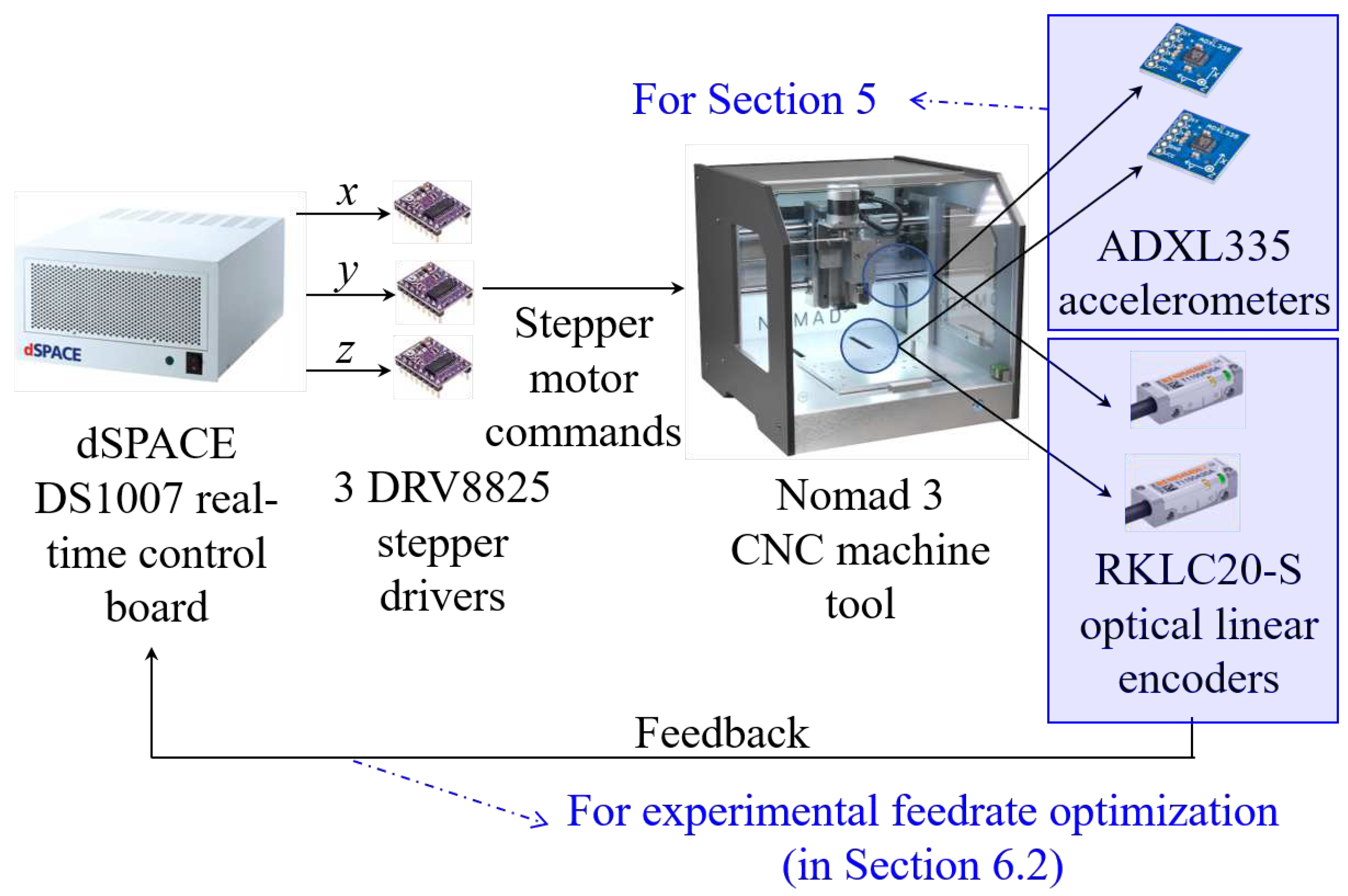
A Nomad 3 three-axis desktop CNC machine tool is chosen as the simulated system, where its setup is shown in Figure 6. To analyze its known uncertainties, the position commands are generated and commanded by dSPACE DS1007 real-time control board running at 500 Hz sampling rate, connected to DRV8825 stepper motor drivers for the x-, y- and z-axes stepper motors. ADXL335 accelerometers are attached on the x- and y-axis gantries to measure the x and y-axes acceleration. The known uncertainties are identified by measuring FRFs, of which the input is a swept sine acceleration command to the stepper motors, and the output is the relative acceleration between the x- and y-axis using the accelerometers. The operating condition under which the FRFs are measured is varied by modifying the input acceleration amplitude at discrete values: 2 m/ s 2 , 3 m/ s 2 and 4 m/ s 2 , and 3 FRFs are measured per each acceleration amplitude to collect a total of N H = 9 FRFs per axes.
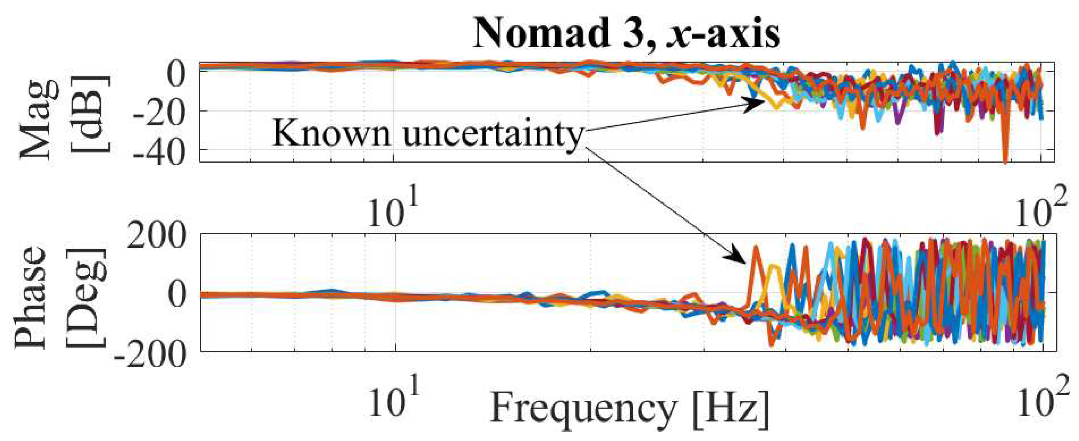
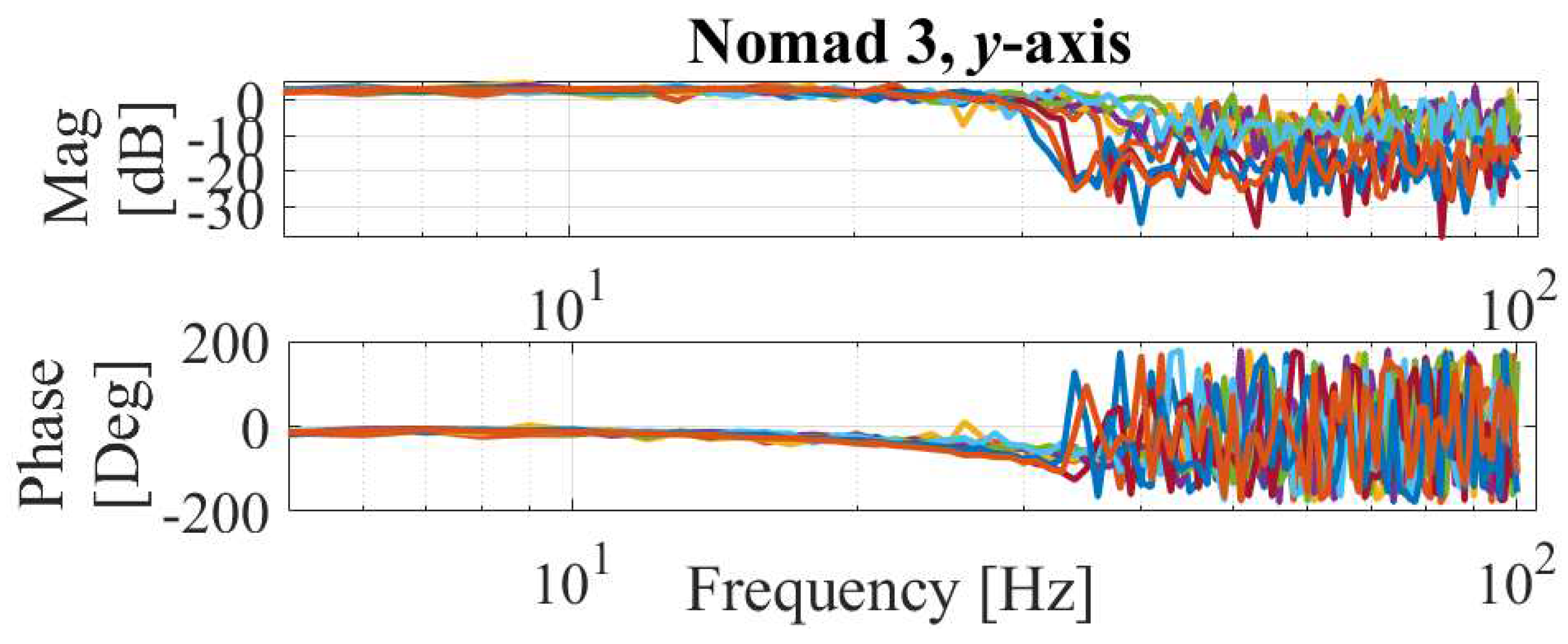
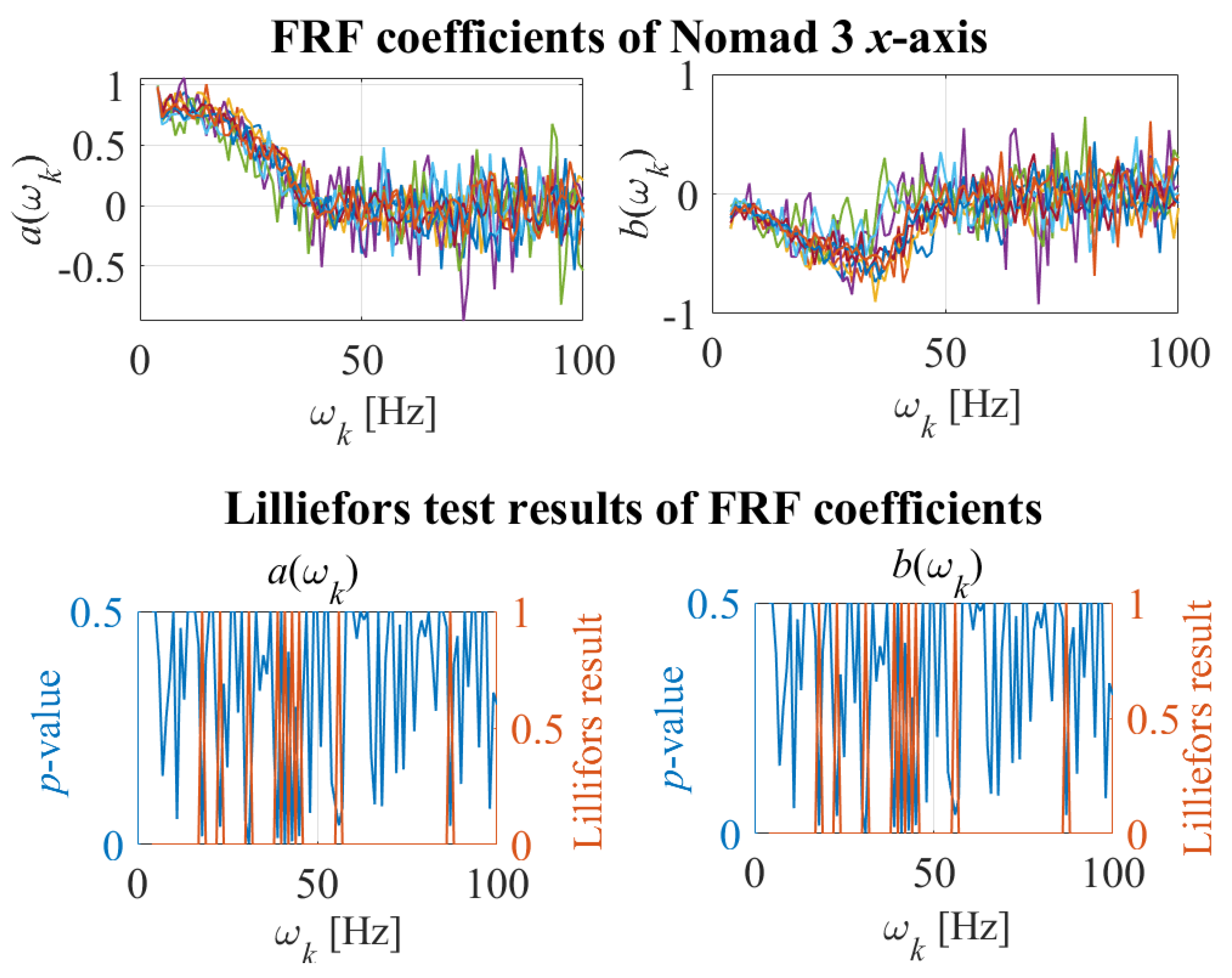
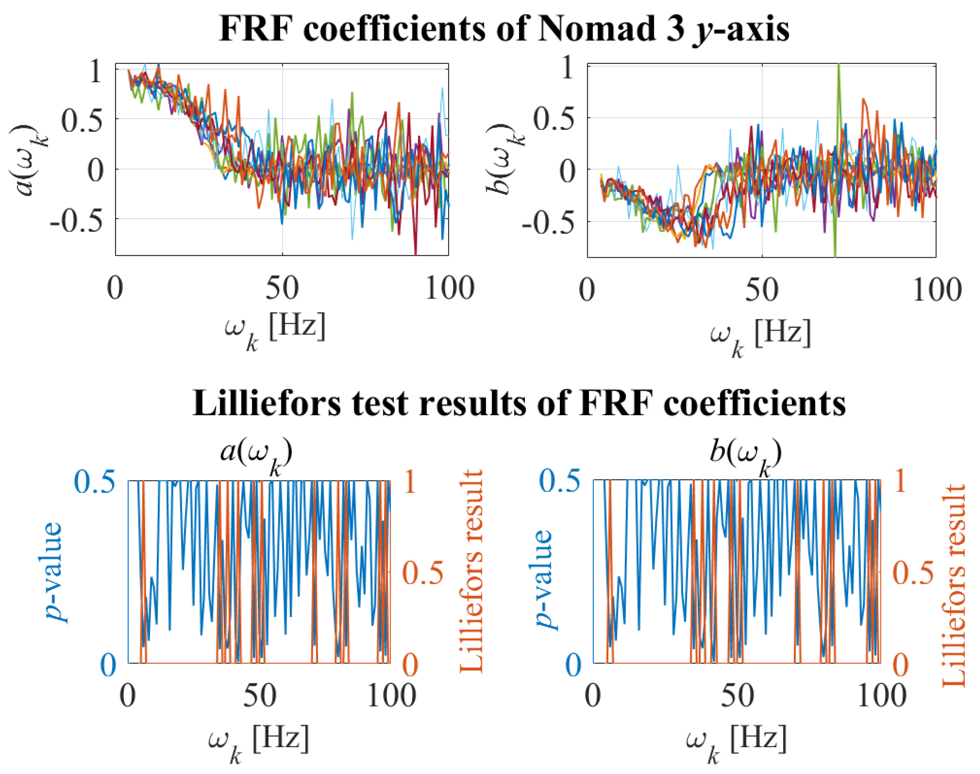
The set of FRFs { H ^ x i } i = 1 9 of the x- and y-axis of the printer are shown in Figure 7 and Figure 8, respectively. The uncertainties in H ^ x are then propagated to h ^ x N ( μ h ^ x , Σ h ^ x ) to initialize μ β and Σ β and construct μ ψ t and Σ ψ t in the physics-informed data-driven digital twin. To validate the hypothesis that the FRF coefficients of { H ^ x } i = 1 9 and { H ^ y } i = 1 9 belong to Gaussian distributions, Lilliefors test [41] is performed on every frequency ω k for k { 1 , 2 , . . . , N H } of a ( ω k ) and b ( ω k ) in x- and y-axis to compute the test decisions at the 5% significance level and p-values. Figure 9 and Figure 10 show the FRF coefficients a ( ω k ) and b ( ω k ) for x- and y-axis, respectively, in the upper plots. The lower plots of Figure 9 and Figure 10 show p-values and Lilliefors test results, where 0 and 1 represent acceptance and rejection of the hypothesis, respectively. The figures imply that Gaussian hypothesis for both a ( ω k ) and b ( ω k ) is accepted at 90% and 88% of the frequencies for the x- and y-axis, respectively. One way to improve the reliability of Lillifors test result is to gather more data of FRFs. However, for the sake of simplicity and computational efficiency, the Gaussian hypothesis will be assumed valid for all frequencies in the following sections.
The output position x is simulated as the sum of motion-induced position x m and force-induced position x f , as
x = x m + x f = h ^ x * x c + x f where h ^ x N ( μ h ^ x , Σ h ^ x ) is sampled at every t and x f ( t ) = A f sin ω f t
where A f = 0.2 and ω f = 733 rad/s (7000 rpm) are chosen.
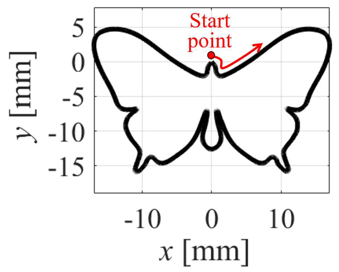
The butterfly trajectory [42] with its contour of the toolpath on the x- and y-axis shown in Figure 11 is selected. For the DD and PIDD methods, n w = 10, n 2 = 3, n 3 = 10 and σ ϵ = 0.01 are selected. For the DD and PIDD methods, stringency η = 95% is selected. V m a x = 30 mm/s, A m a x = 5 m/ s 2 , and contour error limit of E m a x = 0.4 mm are selected for the feedrate optimization. The tolerance violation γ , which will be analyzed for each method, is defined as
γ ( t ) = | ε ( t ) | E m a x i f | ε ( t ) | > E m a x 0 o t h e r w i s e
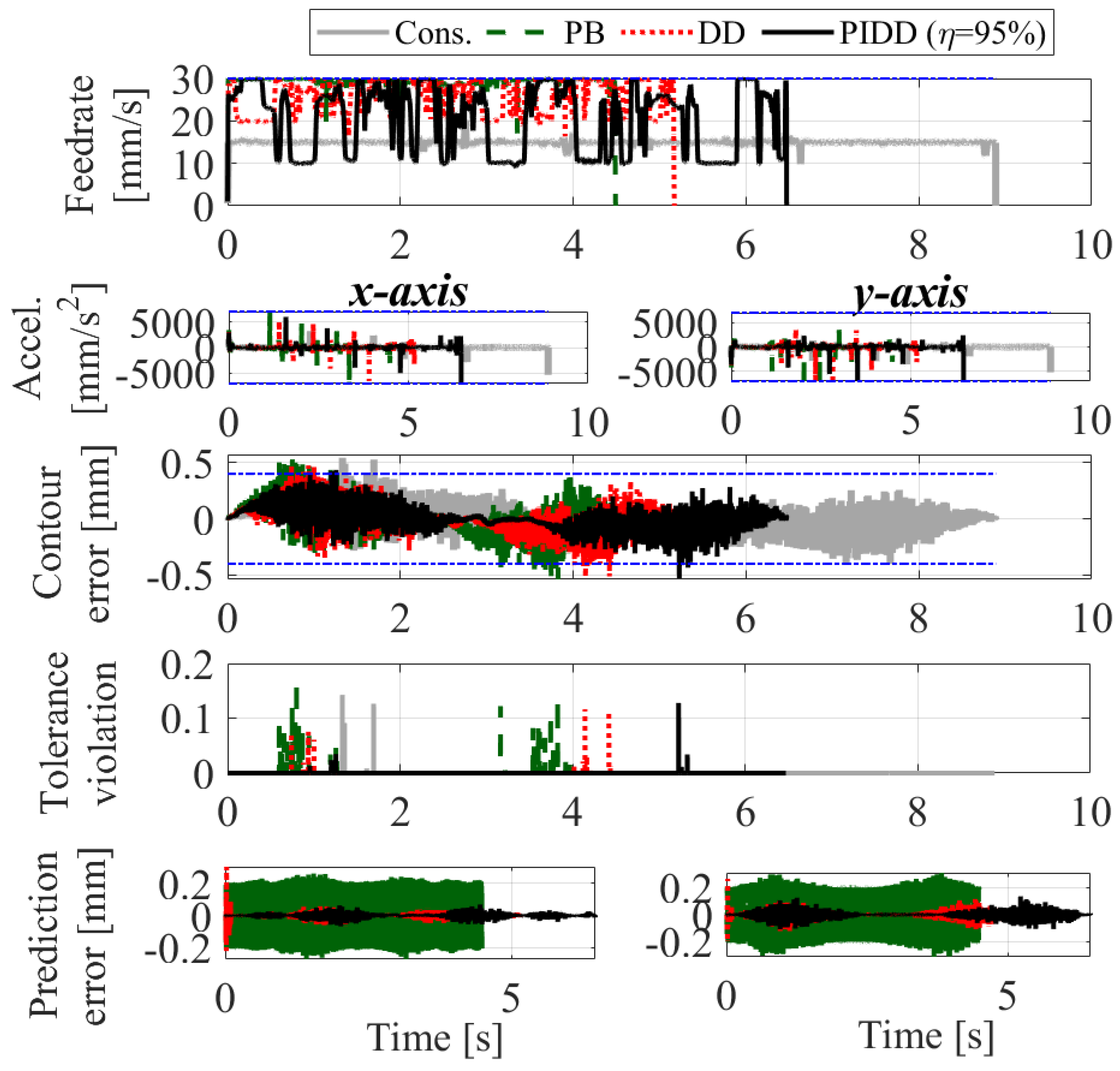
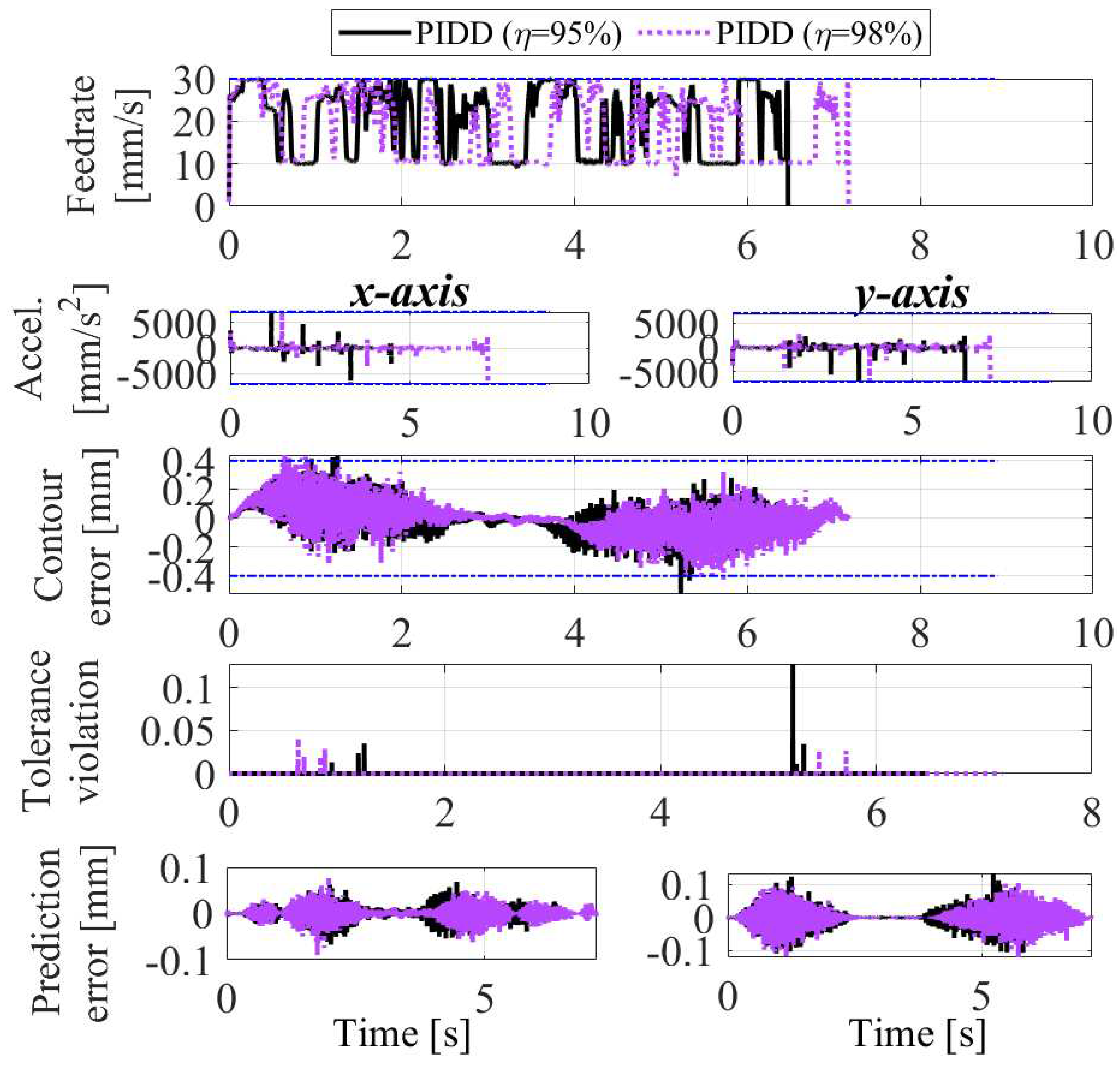
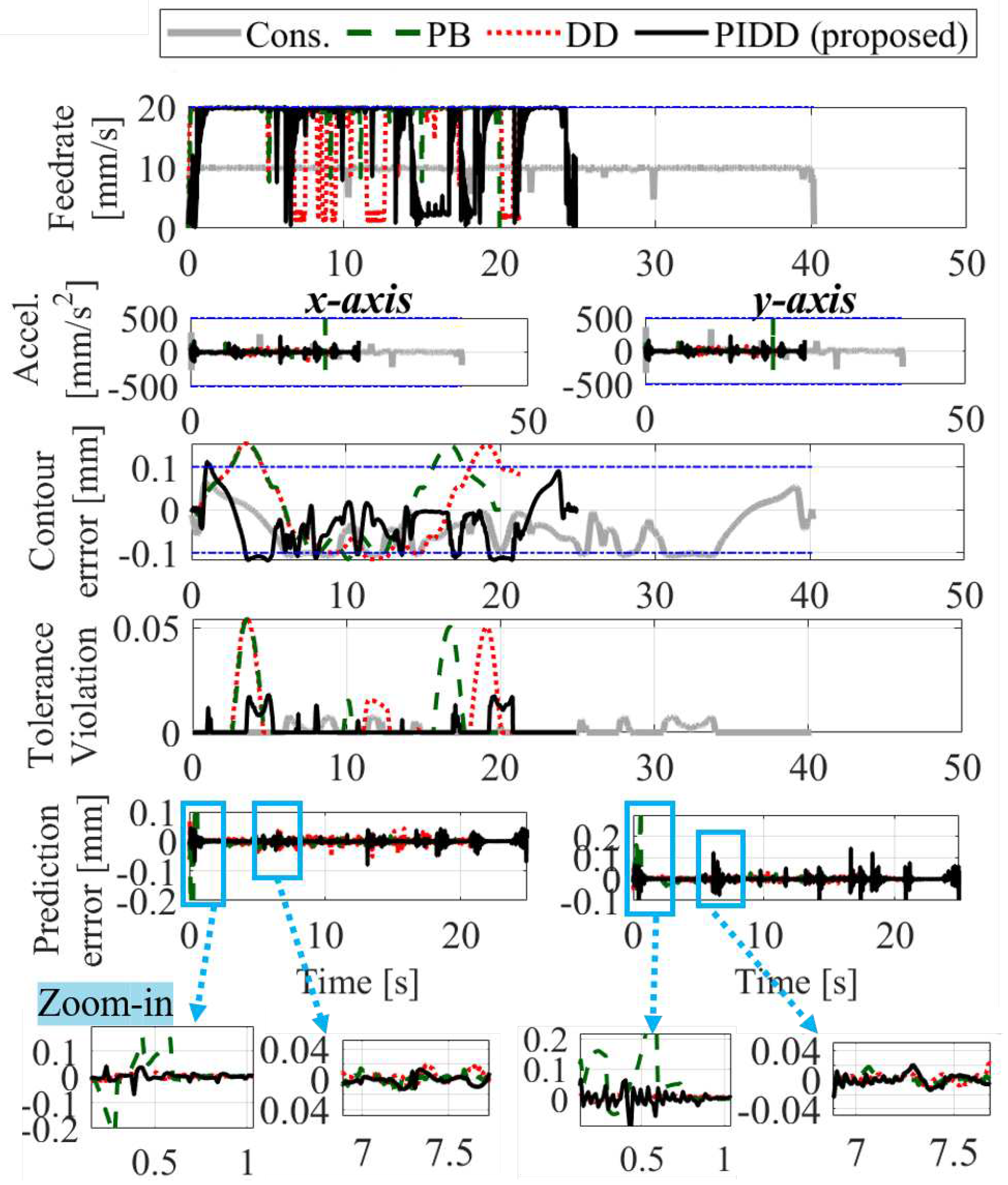
Figure 12 shows the optimized feedrate, acceleration, contour error, tolerance violation and prediction error of all methods. The cycle times and RMS of tolerance violation γ are summarized in Table 1. The PB method is the worst in prediction performance because it is not aware of the unknown uncertainties caused by the force-induced servo error, and hence results in the highest RMS tolerance violation. The DD method improves adherence to the tolerance by learning the unknown uncertainties over time. However, DD method initially suffers from significant prediction error due to its unawareness of known uncertainties. The proposed PIDD method with η = 95% enables restriction of the contour error under the desired stringency by incorporating known uncertainties and learning unknown uncertainties the quickest, which enables it to conservatively stay below the error limit most of the time. Overall, the PIDD method is able to reduce cycle time by 19.3% compared to the conservative approach while maintaining a similar tolerance violation level. To demonstrate the effect of the selection of stringency, Figure 13 compares the commanded feedrate, acceleration, contour error, tolerance violation and prediction error of the PIDD methods using η = 95% and 98%. It is observed that tuning η to a higher level has the effect of making the optimized feedrate more conservative and reducing the error violation.
Note that the proposed PIDD method is not perfect in satisfying the contour error constraints. One reason is that the prediction error is not perfectly zero, and the stringency constraints can only ensure that the worst-case out of η % of contour error distribution is within the tolerance. This issue can be mitigated by increasing η , which will entail more conservative feedrate. Another reason might be due to the nonlinear effects neglected by linearization of the contour error constraint in Eq. (A3) and sub-optimal learning in β introduced by Laplace’s approximation in Eq. (16). These problems can be addressed by applying nonlinear optimization and non-Gaussian Bayesian regression, at the price of higher computational cost.
Figure 12. Feedrate, acceleration, contour error, tolerance violation, and prediction error using conservative (Cons.) physics-based (PB), data-driven (DD) and proposed (PIDD) methods with η = 95% for numerical validation.
Preprints 89465 g012
Figure 13. Feedrate, acceleration, contour error, tolerance violation, and prediction error using the proposed (PIDD) methods with η = 95% (from Figure 12 and η = 98% for numerical validation.
Preprints 89465 g013
Table 1. Cycle times and RMS of tolerance violation γ for conservative (Cons.), physics-based (PB), data-driven (DD) and proposed (PIDD) methods in Figure 12 and Figure 13.
Cons. PB DD PIDD ( η =95%) PIDD ( η =98%)
RMS of γ [ μ m] 2.2 6.6 3.0 1.7 0.8
Cycle time [s] 8.89 4.49 5.17 6.47 7.17

6. Experimental validation

For validation of the proposed approach, two experimental setups are used. The first set of experiments, described in Section 6.1, is carried out on an Ender 3 Pro desktop 3D printer, and the second set of experiments, described in Section 6.2, is carried out on a Nomad 3 desktop CNC machine tool used in Section 5. Demonstration of the proposed method on two experimental setups helps to show its versatility.

6.1. Desktop 3D printer

6.1.1. Experimental setup

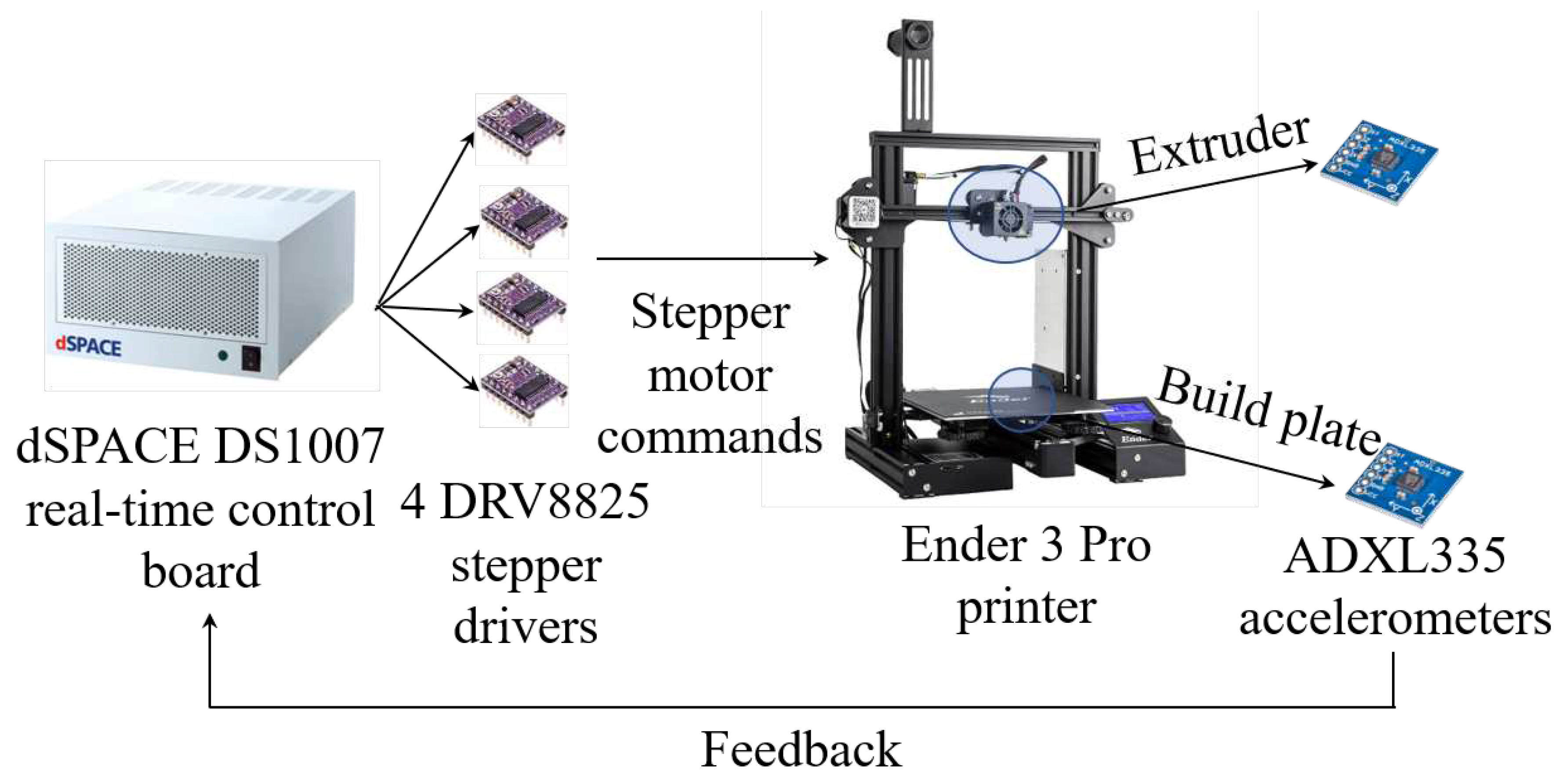
The experimental setup using an Ender 3 Pro desktop 3D printer is shown in Figure 14. The optimization algorithm is implemented on dSPACE 1007 real-time control board running at 500Hz sampling rate, connected to DRV8825 stepper motor drivers for x, y, z and e- axes stepper motors. The measured x and y- axes accelerations from ADXL335 accelerometers are fed back to dSPACE 1007. To deduce the x and y axes displacement from acceleration measurements, a Luenberger state observer [43] is used. The observer gains are chosen such that the dynamics of the observer error (i.e., discrepancy between estimated position using the nominal physics-based model μ h ^ x and observed position) obtains global asymptotic convergence with an observer frequency f o = 15 Hz.

6.1.2. Experimental results

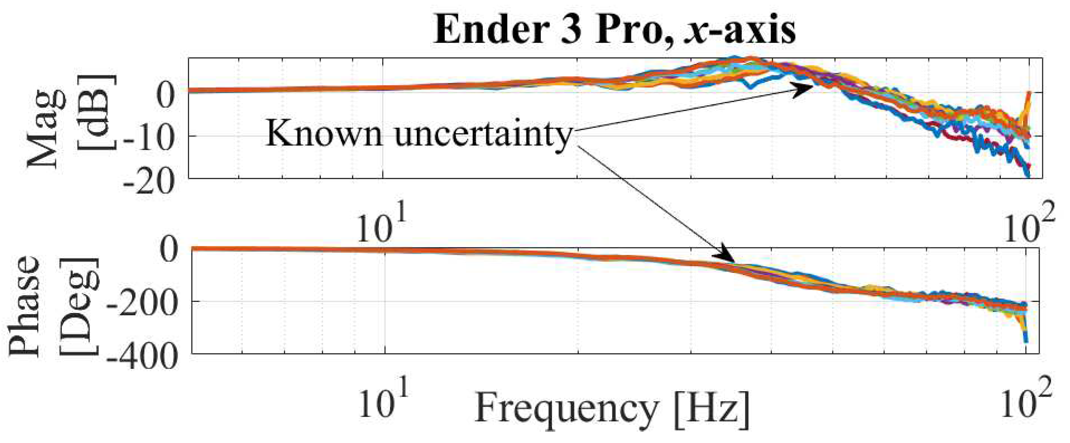
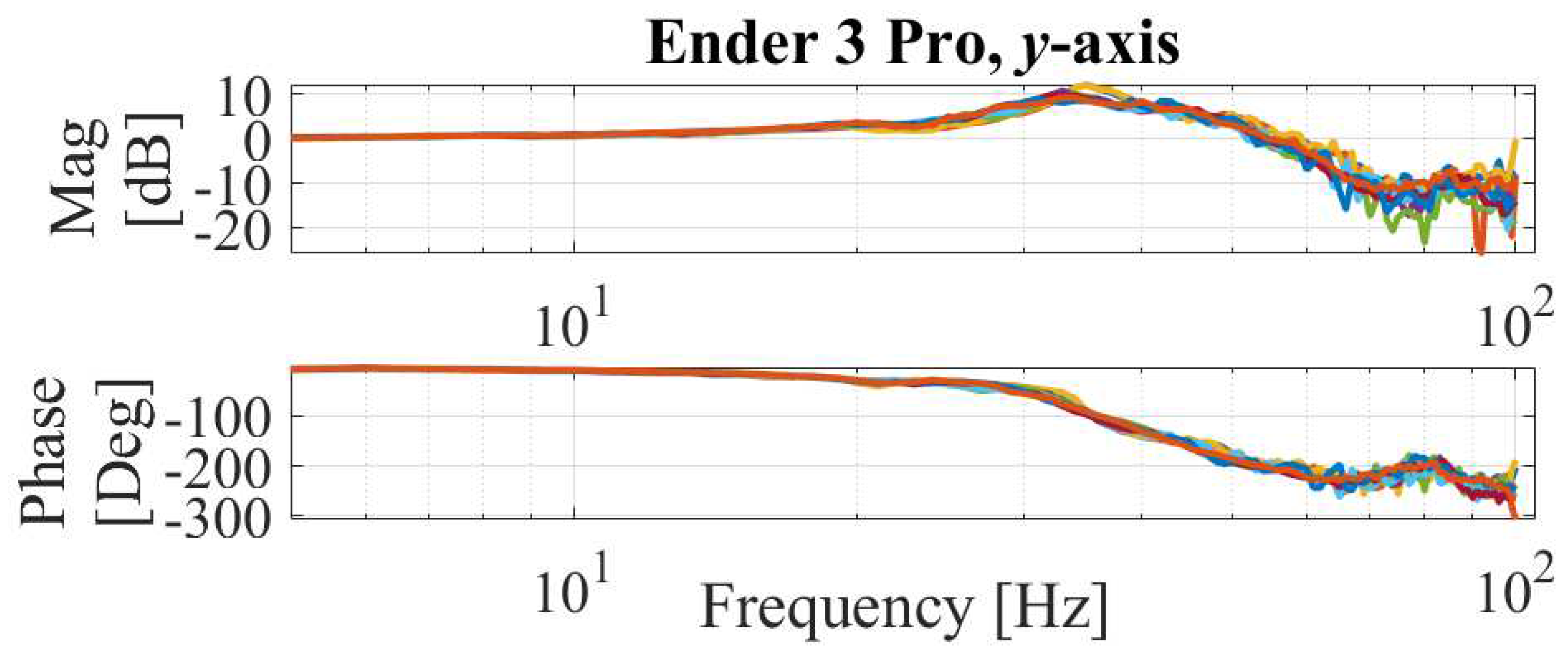
This section validates the proposed approach experimentally using the desktop 3D printer, by comparing its performance with conservative, PB and DD methods. The butterfly toolpath in Figure 11 is used to optimize the feedrate for air-printing (i.e., no material extrusion) and actual printing of the 3D printer. The known uncertainties of x- and y-axis of the printer are incorporated from FRFs in Figure 15 and Figure 16. Similar to Section 5, Lilliefors test is performed on a ( ω k ) and b ( ω k ) of the FRFs in the x- and y-axis to validate the Gaussian assumption at the 5% significance level and p-values, where the hypothesis acceptance rates are computed as 92% and 91% out of all frequencies for the x- and y-axis, respectively. For the DD and PIDD methods, n w = 30, n 2 = 10, n 3 = 30 and σ ϵ = 0.01 are used. For the PIDD method, the desired stringency is selected as η = 95%. For feedrate optimization, V m a x = 70 mm/s, A m a x = 3 m/ s 2 and E m a x = 0.1 mm are chosen.
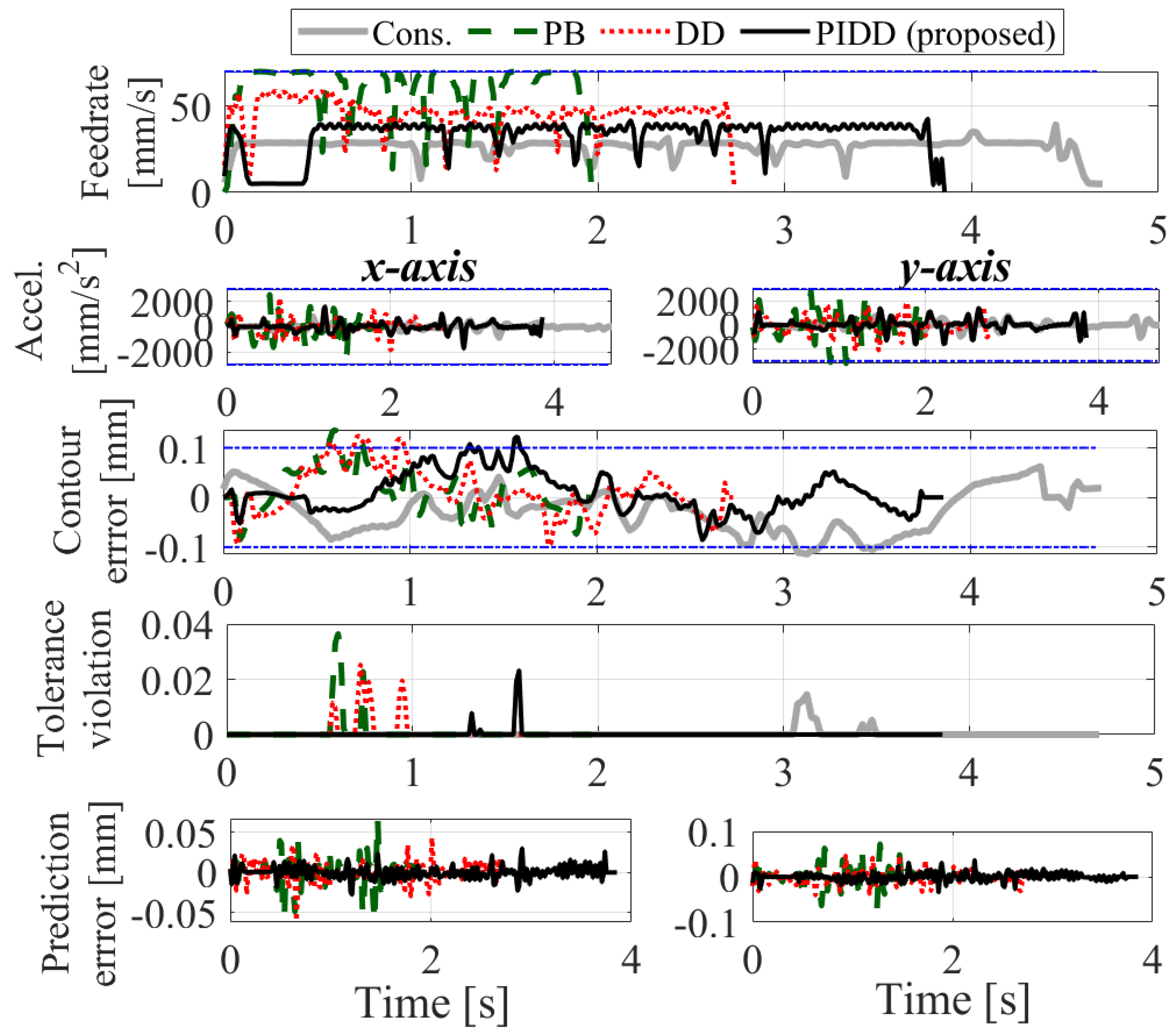
Figure 17 shows the profiles of the optimized feedrate, acceleration, contour error and prediction error of x- and y axis using the conservative, PB, DD and PIDD methods. The RMS prediction errors, cycle times and RMS tolerance violation of all methods are reported in Table 2. The PB approach cannot predict the unknown uncertainties, and hence shows the most significant violation in the contour error. The DD method mitigates the violation by learning the unknown uncertainties, and the PIDD method further improves the accuracy by staying the closest to the tolerance with the desired stringency. As a result, the PIDD method completes the motion 17.8% faster than, while yielding similar contour error tolerance satisfaction as the conservative one.
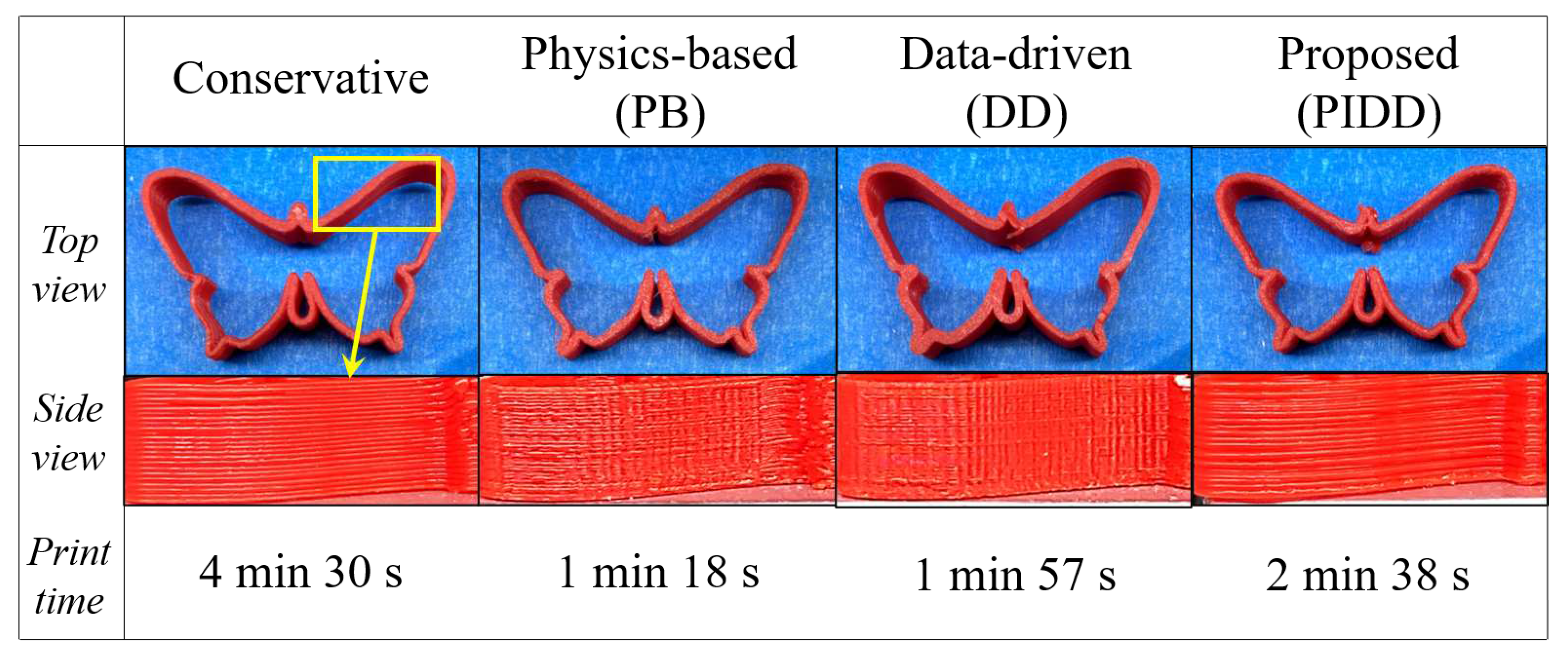
To further validate our findings, a 3D-augmentation of the trajectory in Figure 11 with z-height 8 mm is printed using the same printer. Conservative, PB, DD and PIDD methods are applied at each layer of the print. Figure 18 shows the top and side views of the printed butterflies using the four methods, as well as their print times. The physics-based and data-driven prints show vibration marks in the side view, while the proposed and conservative prints are able to achieve vibration-free surface quality. Overall, the proposed method is able to achieve 15.51% print time reduction compared to the conservative approach while achieving similar print quality.

6.2. CNC machine tool

6.2.1. Experimental setup

For experimental validation, the same experimental setup with the machine tool in Figure 6 in used. The optimization algorithm is implemented on dSPACE 1007 real-time control board running at 500Hz sampling rate, connected to DRV8825 stepper motor drivers for x, y, and z- axes stepper motors. Renishaw RKLC20-S optical linear encoders are attached to the x and y- axes gantries to measure x and y- axes positions that are fed back to dSPACE 1007.

6.2.2. Experimental results

This section validates proposed feedrate optimization using the same set of methods for command generation, which are conservative, PB, DD and the proposed PIDD methods. The same desired butterfly trajectory in Figure 11 is used for air cutting and machining an aluminum workpiece with a 3.175 mm diameter flat-end mill and spindle speed of 7000 rpm. Kinematic limits are set as V m a x = 20 mm/s and A m a x = 0.5 m/ s 2 , and contour error bound is chosen as E m a x = 0.1 mm in the feedrate optimization; n w = 30, n 2 = 2, n 3 = 30 and σ ϵ = 0.01 are used in the DD and PIDD methods. The desired stringency is chosen as η = 95% in the DD and PIDD method.
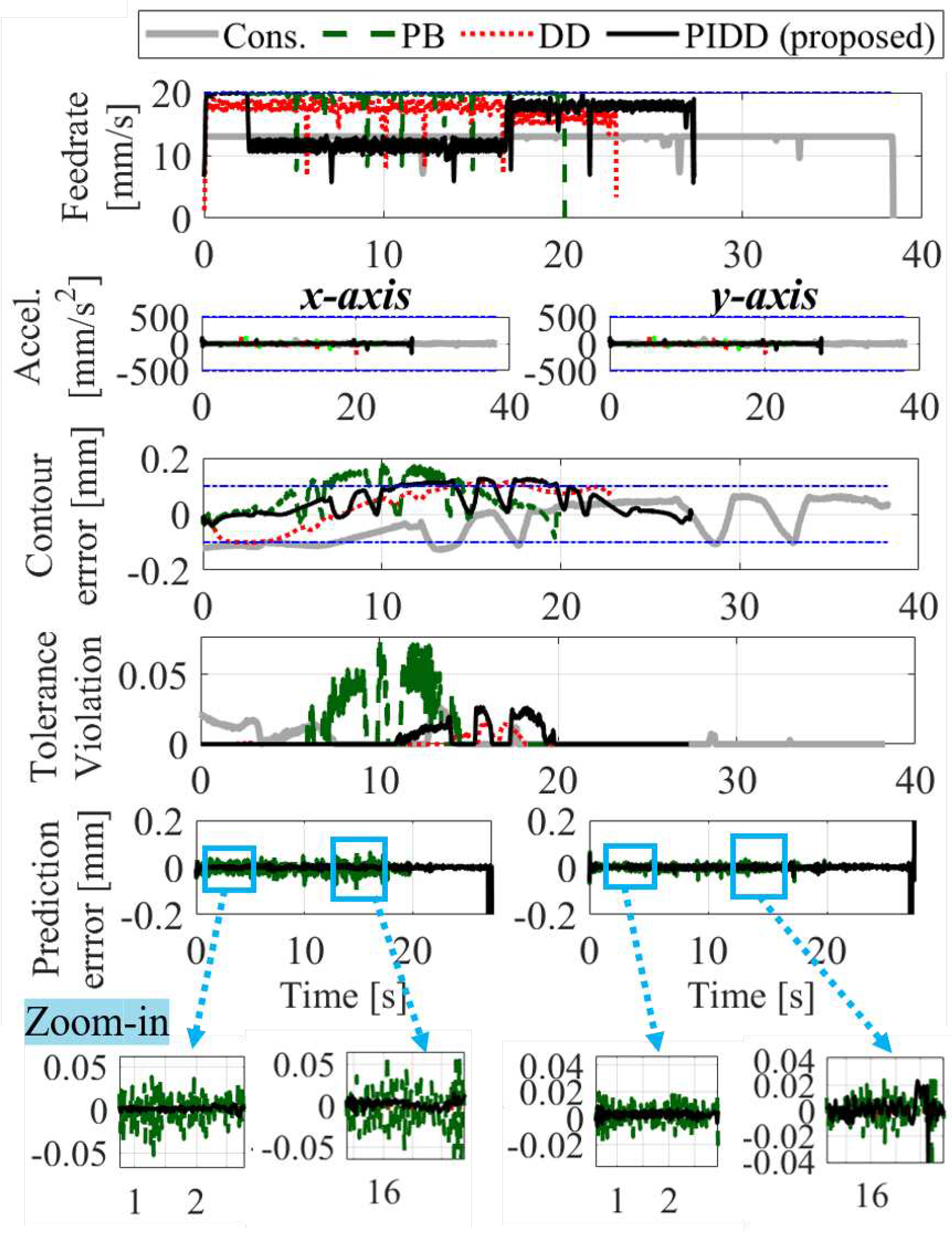
Figure 19 shows the profiles of optimized feedrate, acceleration, contour error, tolerance violation, and prediction error of x- and y-axis in air-cutting using the conservative, PB, DD and PIDD approaches. The PB method frequently violates the tolerance due to unmodeled dynamics, which is caused by the significant prediction error. The DD method slightly improves prediction accuracy, which is further improved in the PIDD method where the contour error is able to be constrained close to the limit using the desired stringency, similar to conservative approach. The proposed PIDD approach completes the motion 38.06% faster than the conservative method, while maintaining a similar level of tolerance adherence. The RMS prediction errors in x- and y-axis, cycle times and RMS tolerance violations of each method are summarized in Table 3.
Figure 20 shows the profiles of optimized feedrate, acceleration, contour error, tolerance violation, and prediction error of x- and y-axis in actual cutting using the conservative, PB, DD and PIDD approaches. Similar to air-cutting, the PB method is worst in constraining the contour error due to unmodeled dynamics and/or cutting force. The DD and PIDD methods reduce the prediction error compared to the PB method and are able to constrain the contour error close to the limit using the desired stringency. However, occasionally, PIDD shows worse performance than DD, which may be due to the difference between measured FRFs when the machine tool is not cutting (shown in Figure 7 and Figure 8) and the FRFs while it is cutting. Research has shown that there can be significant differences between FRFs measured without cutting and those measured while cutting [44]. A possible solution solve this issue is to measure the FRFs and compute known uncertainties during cutting using operational modal analysis, which may be complicated because of FRF’s variability on the operating condition of the cutting tool. Another solution is to discard the known uncertainties when they are inaccurate, i.e., use DD only when PIDD may have errors. Overall, the proposed PIDD approach completes the motion 29.02% faster than the conservative method while maintaining a similar level of tolerance adherence. The RMS prediction errors in x- and y-axis, cycle times and RMS tolerance violations of each method are summarized in Table 3.
Figure 19. Commanded feedrate, acceleration, contour error, tolerance violation, and prediction error (with its zoomed-in images) of conservative, physics-based (PB), data-driven (DD) and proposed (PIDD) approaches in air-cutting.
Preprints 89465 g019
Figure 20. Commanded feedrate, acceleration, contour error, tolerance violation, and prediction error (with its zoomed-in images) of conservative, physics-based (PB), data-driven (DD) and proposed (PIDD) approaches in actual cutting.
Preprints 89465 g020
Table 3. Comparison of RMS prediction errors, cycle times and RMS of tolerance violation γ using conservative (Cons.), physics-based (PB), data-driven (DD) and proposed (PIDD) methods.
Cons. PB DD PIDD
Air-cutting x Pred. Error [ μ m] N/A 17.8 17.5 10.2
y Pred. Error [ μ m] N/A 25.4 15.7 7.2
Cycle time [s] 40.2 20.0 21.1 24.9
RMS of γ [ μ m] 5.0 16.7 16.5 2.3
Cutting x Pred. Error [ μ m] N/A 47.2 17.3 16.7
y Pred. Error [ μ m] N/A 34.2 17.7 18.1
Cycle time [s] 39.4 20.0 23.0 27.2
RMS of γ [ μ m] 6.8 22.2 3.7 7.4
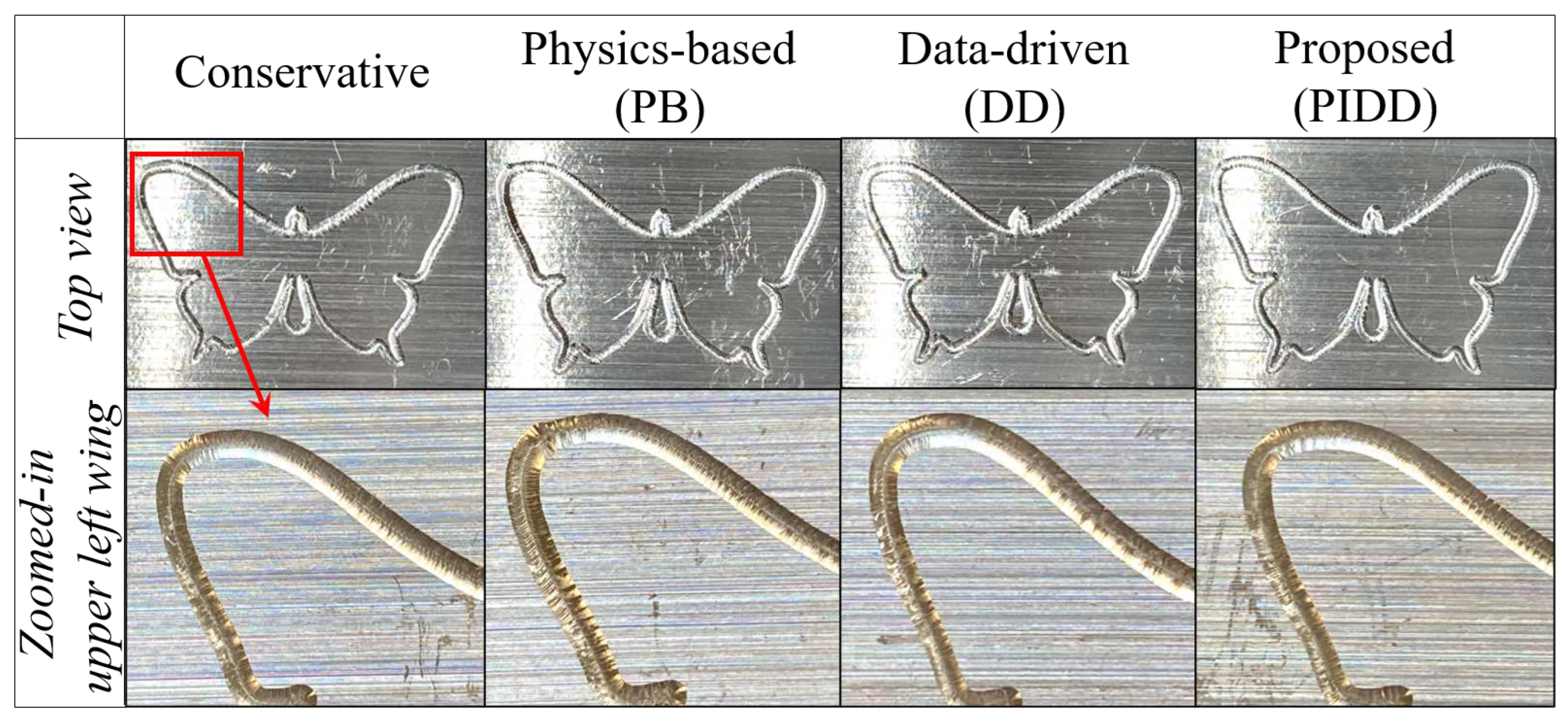
Figure 21 shows the machined surfaces and their zoomed-in images of upper left wing using the trajectories from Figure 20. The surface machined using PB method shows vibration marks, while the DD and PIDD methods mitigate the vibration and achieve similar quality to that of conservative approach.

7. Conclusion and future work

This paper presents an MPC framework and methodology for the intelligent feedrate optimization using an uncertainty-aware digital twin. Its key contributions are summarized as follows.
  • A novel uncertainty-aware digital twin that predicts contour error is proposed. The digital twin is able to incorporate known uncertainty from physics-based models and learn unknown uncertainty using an online data-driven model to predict contour error’s distribution.
  • For the first time, a feedrate optimization with constraints on kinematics and contour error using quantified uncertainty is introduced. The contour error’s uncertainty using digital twin enables the manufacturer to impose stringency constraints, which can replace trial-and-error approach of tuning the tolerance used in practice.
  • We have demonstrated the effectiveness of the intelligent feedrate optimization using uncertainty-aware digital twin, to show up to 38% and 17% cycle time reduction using a desktop CNC machine tool and a desktop 3D printer, respectively, while achieving similar stringency of tolerance to that of the a conservative trial-and-error approach similar to those used in practice.
  • The proposed intelligent feedrate optimization is expected to bring impact in achieving desired quality with higher productivity, using less trial-and-error. It is applicable to any machines that use feed drives, such as coordinate measurement machines (CMMs), and precision machine tools.
As a limitation, the proposed method has made several assumptions in the methodology to enable efficient computation, such as Gaussian distribution of frequency response function for computing the known uncertainty and the linearization of contour error constraints for solving the feedrate optimization as a sequential linear programming problem. The future work will explore more sophisticated (non-Gaussian) uncertainty distributions and nonlinear contour error constraints to improve the accuracy of the digital twin, at the expense of higher computational cost and non-closed form solutions. Furthermore, additional forms of learning to the uncertainty-aware digital twin, such as part-to-part or machine-to-machine learning, will be investigated to improve prediction accuracy.

Acknowledgments

This work is partially funded by the National Science Foundation grants #1931950 and #2054715.

Appendix A. Initialization of μ β and Σ β in Section 3.2

The distribution of the weight β can be initialized and learned more accurately using the feature uncertainty from Eq. (13), where the procedure is described as follows. First, μ β and Σ β are initialized as the priors μ β 0 and Σ β 0 in the 0-th batch using the nominal physics-based model μ h ^ x from Eq. (11). To estimate μ β 0 and Σ β 0 , maximum likelihood estimation (MLE) method is applied on a dataset created offline using a trial desired trajectory x d , t r i a l with length N x that traverses a pre-defined path with conservative kinematics used in practice. The nominal physics-based model μ h ^ x is used to filter x d , t r i a l and formulate x ^ t r i a l . Then, Section 3.1’s framework on deterministic feature vector is borrowed to create multiple datasets consisting of feature vectors and corresponding predictions, i.e., ( ψ 0 , x t r i a l ( 0 ) ) , ( ψ T s , x t r i a l ( T s ) ) , . . . , ( ψ N x T s , x t r i a l ( N x T s ) ) , assuming ψ t is deterministic and ψ t 3 = 0 for all t. Finally, μ β 0 and Σ β 0 can be optimized using MLE as
μ β 0 , Σ β 0 = a r g m i n μ β Σ β i = 0 N x ( 1 2 ( x t r i a l ( i T s ) μ β T ψ i T s ) T ( ψ i T s T Σ β ψ T s i + σ ϵ 2 ) 1 ( x t r i a l ( i T s ) μ β T ψ i T s ) )
where x t r i a l ( t ) is approximated as x ^ t r i a l ( t ) .

Appendix B. Derivation of coefficients c 0 ,c 1 and C 2 in Eq. (16) in Section 3.2

The coefficients c 0 , c 1 and C 2 in Eq. (16) can be derived using 0-th, 1-st and 2-nd derivatives of vector-valued function ln p ( x ( t ) | β ) in Eq. (15) with respect to β , respectively, as
c 0 = 1 2 ( x ( t ) β ¯ T μ ψ t ) T ( β ¯ T Σ ψ t β ¯ + σ ϵ 2 ) 1 ( x ( t ) β ¯ T μ ψ t ) c 1 = 1 2 ( 2 Σ ψ t T μ ψ t x ( t ) β ¯ T β ¯ + 2 μ ψ t μ ψ t T σ ϵ 2 2 Σ ψ t x ( t ) 2 T β ¯ 2 μ ψ t x ( t ) σ ϵ 2 ) · diag ( β ¯ T Σ ψ t T β ¯ + σ ϵ 2 ) 1 C 2 = 1 2 ( 4 Σ ψ t 2 μ ψ t x ( t ) β ¯ T β ¯ β ¯ T + 6 Σ ψ t 2 x ( t ) 2 β ¯ β ¯ T + 12 Σ ψ t μ ψ t x ( t ) σ ϵ 2 β T ¯ 6 Σ ψ t μ ψ t μ ψ t T σ ϵ 2 ) · diag ( β ¯ T Σ ψ t T β ¯ + σ ϵ 2 ) 1
where the local point β ¯ is taken as the prior μ β from the previous window.

Appendix C. Linearization of contour error constraint in Eq. (27) in terms of x ^ d j and y ^ d j

The contour error constraint in Eq. (27) is linearized in terms of x ^ d j and y ^ d j by linearizing the standard deviation term σ ε ˜ ( t ) in Eq. (21) with respect to ψ t and ψ t y using linearization points ψ ¯ t and ψ ¯ t y as
σ ε ˜ ( t ) S x ψ t + S y ψ t y + S 00 + S 01 where S 00 = sin ( θ ( t ) ) 2 ( ψ ¯ t T Σ β ψ ¯ t + σ ϵ 2 ) + cos ( θ ( t ) ) 2 ( ψ ¯ t y T Σ β y ψ ¯ t y + σ ϵ y 2 ) S 01 = 2 sin ( θ ( t ) ) 2 Σ β ψ ¯ t 2 cos ( θ ( t ) ) 2 Σ β ψ ¯ t y S x = 1 S 00 sin ( θ ( t ) ) 2 Σ β S y = 1 S 00 cos ( θ ( t ) ) 2 Σ β y
where ψ ¯ t is formulated via generating the terms x ^ ( t n 2 T s ) x ^ ( t ) in ψ ¯ t 2 by filtering the linearization point f ( p ¯ ) with μ h ^ x . Likewise, ψ ¯ t y is formulated using μ h ^ y .
Finally, let the alterable features in ψ t be ψ t a , and the weights corresponding to the alterable feature in ψ t , i.e., x ^ ( t ) , be denoted as β a and that to the unalterable features ψ t u as β u . The same notations ψ t y u , β y a and β y u will be held for y-axis. Then, by substituting Eq. (21), (25) and (A3) into Eq. (27), the contour error constraint be re-written as
sin ( θ ( t ) ) ( M t x d j μ β u T ψ t u μ β a T ( T x x d j + T 0 x ) ) + cos ( θ ( t ) ) ( M t y d j μ β y u T ψ t y u μ β y a T ( T y y d j + T 0 y ) ) E m a x Φ 1 ( η ) ( S x ψ t u + S x ( T x x d j + T 0 x ) + S y ψ t y u + S y ( T y y d j + T 0 y ) + S 00 + S 01 )
which can be rearranged as linear in terms of x d j and y d j as
U x x d j + U y y d j U 0 where U x = sin ( θ ( t ) ) ( M t μ β a T T x ) + Φ 1 ( η ) S x T x U y = cos ( θ ( t ) ) ( M t μ β y a T T y ) Φ 1 ( η ) S y T y U 0 = sin ( θ ( t ) ) ( μ β u T ψ t u μ β a T T 0 x ) cos ( θ ( t ) ) ( μ β y u T ψ t y u μ β ya T T 0 y ) + E m a x Φ 1 ( η ) ( S x ψ t u + S x T 0 x + S y ψ t y u + S y T 0 y + S 00 + S 01 )
Finally, the contour error constraint in Eq. (A5) is also linear with respect to the decision variable p j using the relationship in Eq. (22).

References

  1. HC, M.; P, W.; K, E.; Y, K. Self-optimizing machining systems. CIRP Annals 2020, 69, 740–763. [CrossRef]
  2. W, F.; XS, G.; CH, L.; K, Z.; Q, Z. Time-Optimal Interpolation for Five-Axis CNC Machining along Parametric Tool Path Based on Linear Programming. Int J Adv Manuf Technol 2013, 69, 1373–1388. [CrossRef]
  3. K, E.; QGC, C.; Zhao MY, B.X.; XS, G. Linear Programming and Windowing Based Feedrate Optimization for Spline Toolpaths. CIRP Annals 2017, 66, 393–396. [CrossRef]
  4. A, B.; J, D. Feedrate Optimization for Smooth Minimum-Time Trajectory Generation with Higher Order Constraints. Int J Adv Manuf Technol 2016, 82, 1029–1040. [CrossRef]
  5. Q, Z.; SR, L. Efficient Computation of Smooth Minimum Time Trajectory for CNC Machining. Int J Adv Manuf Technol 2013, 68, 683–692. [CrossRef]
  6. S, T.; B, S. Real-time trajectory generation for 5-axis machine tools with singularity avoidance. CIRP Annals 2020, 69, 349–352. [CrossRef]
  7. S, T.; B, S. Online interpolation of 5-axis machining toolpaths with global blending. International Journal of Machine Tools and Manufacture 2022, 175, 103862. [CrossRef]
  8. M, C.; J, X.; Y, S. Adaptive feedrate planning for continuous parametric tool path with confined contour error and axis jerks. The International Journal of Advanced Manufacturing Technology 2017, 89, 1113–1125. [CrossRef]
  9. J, D.; JA, S. Optimal feed-rate scheduling for high-speed contouring. J. Manuf. Sci. Eng. 2007, 129, 63–76. [CrossRef]
  10. W, F.; XS, G.; CH, L.; K, Z.; Q, Z. Time-optimal interpolation for five-axis CNC machining along parametric tool path based on linear programming. The International Journal of Advanced Manufacturing Technology 2013, 69, 1373–1388. [CrossRef]
  11. H, E.; I, L.; B, O. Feedrate scheduling strategies for free-form surfaces. International Journal of Machine Tools and Manufacture 2006, 46, 747–757. [CrossRef]
  12. L, Z.; J, F.; Y, W.; M, C. Feedrate scheduling strategy for free-form surface machining through an integrated geometric and mechanistic model. International Journal of Advanced Manufacturing Technology 2009, 40, 740–763. [CrossRef]
  13. SD, M.; Y, A. Virtual cutting and optimization of three-axis milling processes. International Journal of Machine Tools and Manufacture 2008, 48, 1063–1071. [CrossRef]
  14. ND, R.; BK, F.; RB, J. Efficient NC machining using off-line optimized feedrates and on-line adaptive control. 2002, Vol. 3641, pp. 181–191. [CrossRef]
  15. H, E.; I, L.; M, K. Free-form surface machining and comparing feedrate scheduling strategies. Machining Science and Technology 2007, 11, 117–133. [CrossRef]
  16. HS, P.; B, Q.; DV, D.; DY, P. Development of smart machining system for optimizing feedrates to minimize machining time. Journal of Computational Design and Engineering 2018, 5, 299–304. [CrossRef]
  17. Y, A.; Kersting P, B.D.; E, B.; B, D.; I, L. Virtual process systems for part machining operations. CIRP Annals 2014, 63, 585–605. [CrossRef]
  18. HU, L.; DW, C. An intelligent feedrate scheduling based on virtual machining. The International Journal of Advanced Manufacturing Technology 2003, 22, 873–882.
  19. BK, F.; RB, J.; JG, H. Robust feedrate selection for 3-axis NC machining using discrete models. J. Manuf. Sci. Eng. 2001, 123, 214–224. [CrossRef]
  20. Y, A.; SD, M. Virtual high performance milling. CIRP annals 2007, 56, 81–84. [CrossRef]
  21. JH, K.; WS, Y.; DW, C. Off-line feed rate scheduling using virtual CNC based on an evaluation of cutting performance. Computer-Aided Design 2003, 35, 383–393. [CrossRef]
  22. SD, M.; Y, A. Virtual simulation and optimization of milling applications—part II: optimization and feedrate scheduling. [CrossRef]
  23. HY, F.; N, S. Integrated tool path and feed rate optimization for the finishing machining of 3D plane surfaces. International Journal of Machine Tools and Manufacture 2000, 40, 1557–1572. [CrossRef]
  24. CM, B.; M, L.; P, B. A model-based adaptive controller for chatter mitigation and productivity enhancement in CNC milling machines. Robotics and Computer-Integrated Manufacturing 2016, 40, 34–43. [CrossRef]
  25. P, Q.; M, W.; L, S. Feed Rate Variation Strategy for Semi-Conical Shell Workpiece in Ball Head End Milling Process. Applied Sciences 2020, 10, 9135. [CrossRef]
  26. J, Y.; D, A.; Y, A. A feedrate scheduling algorithm to constrain tool tip position and tool orientation errors of five-axis CNC machining under cutting load disturbances. CIRP journal of Manufacturing Science and Technology 2018, 23, 78–90. [CrossRef]
  27. Y, A.; J, Y.; ZM, K. Virtual prediction and constraint of contour errors induced by cutting force disturbances on multi-axis CNC machine tools. CIRP Annals 2019, 68, 377–380. [CrossRef]
  28. H, K.; CE, O. Simultaneous servo error pre-compensation and feedrate optimization with tolerance constraints using linear programming. Int J Adv Manuf Technol 2020, 109, 809–821. [CrossRef]
  29. H, K.; CE, O. Accurate and computationally efficient approach for simultaneous feedrate optimization and servo error pre-compensation of long toolpaths—with application to a 3D printer. The International Journal of Advanced Manufacturing Technology 2021, 115, 2069–2082. [CrossRef]
  30. JB, R.; DQ, M.; M, D. Model predictive control: theory, computation, and design; Vol. 2, Madison, WI: Nob Hill Publishing.
  31. H, K.; C, O. Intelligent feedrate optimization using a physics-based and data-driven digital twin. CIRP Annals. 2023, pp. 308–322. [CrossRef]
  32. YC, C.; CW, C.; TC, T. Near time-optimal real-time path following under error tolerance and system constraints. CIRP Annals 2018, 140, 071004. [CrossRef]
  33. S, B.; D, L.M.; A, R.; J, L. Data-driven Reference Trajectory Optimization for Precision Motion Systems. arXiv preprint 2205.15694 2022.
  34. L, R.; I, L.; ED, K.; HC, M. Safe optimization for feedrate scheduling of power-constrained milling processes by using Gaussian processes. Procedia CIRP 2021, 99, 127–132. [CrossRef]
  35. R, K.; G, R.; Z, S. Minimizing negative transfer of knowledge in multivariate gaussian processes: A scalable and regularized approach. IEEE Transactions on Pattern Analysis and Machine Intelligence 2020, 43, 3508–3522. [CrossRef]
  36. CH, C.; M, D.; CE, O. A linear hybrid model for enhanced servo error pre-compensation of feed drives with unmodeled nonlinear dynamics. CIRP Annals 2021, 70, 301–304. [CrossRef]
  37. D, L.; C, M.; MC, G. Model Predictive Contouring Control for Biaxial Systems. IEEE Transactions on Control Systems Technology 2012, 2, 552–559. [CrossRef]
  38. DJ, M. Information theory, inference and learning algorithms; Cambridge university press, 2003.
  39. JB, R. Model predictive control technology. 1999, Vol. 1, pp. 662–676.
  40. DJ, G.; K, E. Accurate control of ball screw drives using pole-placement vibration damping and a novel trajectory prefilter. Precision Engineering 2013, 37, 308–322. [CrossRef]
  41. HW, L. On the Kolmogorov-Smirnov test for normality with mean and variance unknown. Journal of the American Statistical Association 1967, 62, 339–402. [CrossRef]
  42. S, Y.; AH, G.; X, L.; CE, O. Pre-Compensation of Servo Contour Errors Using a Model Predictive Control Framework. Int J Mach Tool Manu 2015, 98, 50–60. [CrossRef]
  43. DG, L. An Introduction to Observers. IEEE Trans. On Automatic Control 1971, 16, 596–602. [CrossRef]
  44. I, Z.; V, S. Estimation of machine-tool dynamic parameters during machining operation through operational modal analysis. International Journal of Machine Tools and Manufacture 2009, 49, 945–957. [CrossRef]
Figure 1. Diagram of intelligent feedrate optimization using an uncertainty-aware digital twin. A manufacturer provides a part tolerance and stringency (i.e., the tolerance for quality constraint violation under uncertainty). The intelligent machine leverages an uncertainty-aware digital twin to optimize feedrate while satisfying the tolerance and stringency requirements.
Preprints 89465 g001
Figure 3. Flowchart of intelligent feedrate optimization using a deterministic digital twin with physics-based and data-driven servo models (y-axis omitted for simplicity).
Preprints 89465 g003
Figure 4. Batches j 1 and j defined on a discrete-time domain.
Preprints 89465 g004
Figure 6. Experimental setup for Section 5 and Section 6.2.
Preprints 89465 g006
Figure 7. Frequency response functions of the Nomad 3’s x-axis showing the known uncertainty obtained under different input acceleration amplitudes.
Preprints 89465 g007
Figure 8. Frequency response functions of the Nomad 3’s y-axis showing the known uncertainty obtained under different input acceleration amplitudes.
Preprints 89465 g008
Figure 9. Upper plot: FRF coefficients a ( ω k ) and b ( ω k ) of Nomad 3 x-axis; lower plot: p-value and accept/reject results of Lilliefors test of FRF coefficients.
Preprints 89465 g009
Figure 10. Upper plot: FRF coefficients a ( ω k ) and b ( ω k ) of Nomad 3 y-axis; lower plot: p-value and accept/reject results of Lilliefors test of FRF coefficients.
Preprints 89465 g010
Figure 11. Desired toolpath.
Preprints 89465 g011
Figure 14. Experimental setup for Section 6.1.
Preprints 89465 g014
Figure 15. Frequency response functions of the Ender 3 Pro’s x-axis showing the known uncertainty obtained under different input acceleration amplitudes.
Preprints 89465 g015
Figure 16. Frequency response functions of the Ender 3 Pro’s y-axis showing the known uncertainty obtained under different input acceleration amplitudes.
Preprints 89465 g016
Figure 17. Commanded feedrate, acceleration, contour error, tolerance violation and prediction error using conservative (Cons.), physics-based, data-driven and proposed approaches in air-printing.
Preprints 89465 g017
Figure 18. Top and side views of 3D-printed butterfly models using conservative, physics-based, data-driven and proposed approaches and their print times.
Preprints 89465 g018
Figure 21. Machined parts and the zoomed-in images of upper left wing using conservative, physics-based (PB), data-driven (DD) and proposed (PIDD) approaches
Preprints 89465 g021
Table 2. Comparison of RMS prediction errors, cycle times and RMS of tolerance violation γ using conservative (Cons.), physics-based (Physics.), data-driven (Data.) and proposed methods in air-printing.
Cons. Physics. Data. Proposed
x Pred. Error [ μ m] N/A 37.4 22.1 18.1
y Pred. Error [ μ m] N/A 31.7 23.9 19.3
Cycle time [s] 4.70 1.97 2.73 3.86
RMS of γ [ μ m] 1.8 5.5 3.9 1.9
Disclaimer/Publisher’s Note: The statements, opinions and data contained in all publications are solely those of the individual author(s) and contributor(s) and not of MDPI and/or the editor(s). MDPI and/or the editor(s) disclaim responsibility for any injury to people or property resulting from any ideas, methods, instructions or products referred to in the content.
Copyright: This open access article is published under a Creative Commons CC BY 4.0 license, which permit the free download, distribution, and reuse, provided that the author and preprint are cited in any reuse.
Prerpints.org logo

Preprints.org is a free preprint server supported by MDPI in Basel, Switzerland.

Subscribe

© 2024 MDPI (Basel, Switzerland) unless otherwise stated