

Submitted:
11 May 2026
Posted:
12 May 2026
You are already at the latest version
Abstract
We discover a synchronization admissibility boundary defined solely by the states of oscillators. The boundary is independent of structure and determines whether any two oscillators share a cluster in real time, unifying global synchronization, cluster partition, and the real-time onset of synchronization loss. This uniformity has been validated through dozens of adversarial tests. Mathematical proofs show that this boundary is mathematically equivalent to the constraint that the synchronous frequency must be a real number. This constraint is a direct corollary of a cornerstone of physics long taken for granted: all measurable physical quantities are real numbers. This equivalence reveals that the synchronous admissibility boundary (a key function) emerges directly from the principle that is logically prior to any specific structure.
Keywords:
synchronization admissibility boundary
; the real number constraint
; emergence
Introduction
The collective behavior of coupled nonlinear oscillators, from neuronal firing1 to power grids, is governed by synchronization2. A fundamental question in the study of coupled oscillators is: what determines the boundary of synchronization? The conventional approaches answers this question by focusing on the system's structure: its network topology and system parameters3–5. In physics, the topology is typically quantified using an adjacency matrix of network, and parameters include edge weights, oscillator inertia, and damping. The view serves as the cornerstone for constructing analytical frameworks ranging from graph theory to master stability functions3,5, and recent research continues to reinforce it across various synchronization phenomena6,7. Conventional approaches built on this premise have achieved considerable success, but they all share a crucial dependency: they require complete structural information.
However, interactions in the real world cannot always be observed directly or clearly. In such cases, traditional approaches risk failing. We are forced to confront a series of deeper, often unasked questions8: Is this reliance necessary? If not, how should we understand the emergence of synchronization?
To explore these questions, we depart from conventional structure-based analysis and adopt a different approach: we directly analyze the states of oscillator systems at the limit of synchronous stability to determine what special characteristics they possess?
Guided by this aim, we combined physical intuition with the analyses of simulation data and geometric analogies to phasor diagrams. This approach led to the discovery of an elegant equation. Within the testing framework of this paper, this equation can uniformly distinguish between global synchronization9 and cluster synchronization10, including the timing of synchronization clusters split11 and the members within each cluster. The key feature of this boundary is that its mathematical form contains no terms pertaining to network adjacency matrices, edge weights, or oscillator parameters. That is, the boundary (the function) is independent of the structure. This independence reveals a pathway to assess admissibility that circumvents the requirement for structural knowledge. Initially, it was merely an observational finding. However, through a series of adversarial tests across two structure disparate test systems, this equation demonstrated robust discriminatory power. These systems differ significantly in terms of the number of oscillators, the number of edges, and the adjacency matrix; furthermore, the inertia, damping, and edge weights of the oscillators within each system also vary. Furthermore, through a series of mathematical equivalence proofs, we have established that this boundary is mathematically equivalent to the constraint that the synchronous angular frequency must be a real number. This constraint, considered prior to any specific structure, arises directly from a cornerstone of physics: measurable physical quantities must be real numbers.
As a further direct corroboration, we explored the system's behavior near the boundary and discovered a novel self-organizing emergent phenomenon. This is a type of spontaneous synchronization that occurs only near critical points. Therefore, it exhibits structure-independent properties.
By demonstrating that the synchronization admissibility boundary is independent of structure, our findings show that this key function can be determined without knowledge of network topology or system parameters. Furthermore, practical methods that establish a direct link between boundaries and fundamental principles of physics may provide inspiration for related interdisciplinary research.
Results and discussion
Boundary equation and its verification
Our exploration followed a classic and productive path in physics research: “discover; validate; explain.”
Discovery:
What makes the synchronization critical state so special5,12,13? To answer this question, we conducted an in-depth analysis of the simulation data from the standard power grid test system. We recorded the time series data of oscillator amplitude and angular frequency and classified the outcome as stable or unstable on the basis of time stability (see S1 in the supplemental material). In these cases, a striking regularity emerged: When the system is in a critical state, the amplitude and angular frequency of the oscillator pair exhibit a specific geometric relationship. This relationship can be expressed by an elegant equation (see S1 in the supplemental material for details). This equation is used to describe the synchronization admissibility boundary:

 denotes the oscillation amplitude of the Kth oscillator, and
 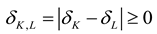 denotes the angle difference between
  and
and  .
. 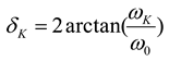 denotes the angle of angular frequency of the Kth oscillator (not the phase angle), and synchronization corresponds to
  .
.  denotes the angular frequency of Kth oscillator and
  is the common angular frequency of the system.
While frameworks5,14 have shown that synchronization boundaries typically depend on network structure, Eq. (1) is determined solely by the oscillator’s amplitude and the angle of angular frequency. Consequently, the boundary equation is independent of structure. This independence implies that the boundary equation is generally applicable to oscillator systems with different structures. Furthermore, this boundary (key function) can be discovered independently of structure, thereby providing a counterexample to the view that the “structure determines function” principle is a necessary foundation for understanding collective behavior4,5. The subsequent verification aims to demonstrate the validity of this boundary and its independence from structure.
Visual verification:
Any test can only indicate whether the oscillators are in sync, but cannot directly identify the boundary, since the boundary is not a single state but a set of critical points. Therefore, we locate it by simulating the stability of the synchronous cluster: by gradually increasing the disturbance intensity, we observe how the system transitions from a stable state to a split state in the form of a synchronous cluster. Here, “admissibility” refers to whether it is physically permissible for two oscillators to belong to the same synchronization cluster: when a point 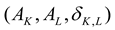 lies inside the boundary, the two oscillators K and L belong to the same cluster; outside the boundary, they do not. Global synchronization corresponds to a special type of synchronization cluster in which all oscillators belong to the same cluster, while the moment of cluster splitting and its division are marked by points crossing the boundary.
lies inside the boundary, the two oscillators K and L belong to the same cluster; outside the boundary, they do not. Global synchronization corresponds to a special type of synchronization cluster in which all oscillators belong to the same cluster, while the moment of cluster splitting and its division are marked by points crossing the boundary.Eq. (1) presents a boundary for a pair of oscillators. Directly applying Eq. (1) to multibody problems introduces a fundamental challenge: evaluating  pairs of oscillators simultaneously is necessaty. This characteristic leads to the curse of dimensionality and renders visual verification of the synchronization admissibility boundary impossible.
pairs of oscillators simultaneously is necessaty. This characteristic leads to the curse of dimensionality and renders visual verification of the synchronization admissibility boundary impossible.To address this challenge, we introduce the meta-oscillator transform (see S2.4 in the supplementary material). This operation reorders the oscillators on the basis of their instantaneous angular frequency, creating a new sequence in which only adjacent pairs (K and L=K+1) need to be examined. For a system with n meta-oscillators, the state is represented by n-1 points (see Figure 2b). The meta-oscillator framework reduces the analysis to just n−1 adjacent pairs. Critically, we prove that this transformation preserves synchronization admissibility, which ensures equivalence in the admissibility states between the oscillator and meta-oscillator systems within the validation framework of this paper (see S2.5 in the supplementary material). This equivalence allows us to directly verify the validity of the boundary conditions by comparing the admissibility results of the meta-oscillators (Figure 1 and Figure 2) with the numerical simulation results.
As shown in Figure 1a, Eq. (1) can be visualized as a surface in a three-dimensional (3D) space, dividing that space into two regions. When the system corresponds to the inner region, synchronization is admissible. Otherwise, it is inadmissible. Therefore, the surface provides a definitive geometric criterion for oscillator system admissibility. On the other hand, because the variables  ,
,  , and
, and  serve as the axes of the coordinate system, the surface defined by Eq. (1) is geometrically fixed. In other words, changes to the structure do not alter this surface. This finding intuitively demonstrates that the boundary is independent of the structure. The central thesis of this paper thus reduces to a testable question: does this fixed surface effectively determine admissibility across different structures?
, , and serve as the axes of the coordinate system, the surface defined by Eq. (1) is geometrically fixed. In other words, changes to the structure do not alter this surface. This finding intuitively demonstrates that the boundary is independent of the structure. The central thesis of this paper thus reduces to a testable question: does this fixed surface effectively determine admissibility across different structures?Next, we experimentally verify that the synchronous admissibility boundary is described by Eq. (1) and is independent of the structure. Rather than testing the boundary equation under average or near-linear conditions, we subjected it to a series of adversarial tests. These tests include the following: 1, two standard test systems that differ significantly in scale, topology, and component heterogeneity; 2, heterogeneous oscillator parameters within each system; 3, different edge weights; 4, strong disturbances at multiple distinct nodes; and 5, dynamics that are mathematically equivalent to the second-order Kuramoto model. If a structure-independent boundary remains valid under such a battery of complex conditions, its claim to validity is substantially strengthened. The following three phenomena should be interpreted with this stringent standard in mind: 1) it distinguishes between admissible and inadmissible states [see Figure 1b and Figure 2a], 2) it captures the real-time transition in admissibility [see Figure 1c and Figure 2b], and 3) it explains partial synchronization patterns [see Figure 1f and Figure 2e]. Importantly, achieving a unified understanding of these relatively independent phenomena is a focus of current research10,15, and we provide a promising single criterion for this purpose.
To test the boundary, a test system (10-oscillator) was used. A strong disturbance occurred at node 18. The data in Figure 1 were obtained from numerical simulation experiments designed to validate Eq. (1).  represents the disturbance duration, and
 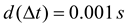 denotes the step size of the variation in .
represents the disturbance duration, and denotes the step size of the variation in .(a). Visualization of the admissibility boundary. The admissibility boundary in Eq. (1) (blue surface) and the pink planes 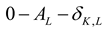 ,
, 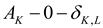 and
and  collectively define the boundaries and enclose the admissibility domain. The identical boundary form enables a unified admissibility assessment.
, and collectively define the boundaries and enclose the admissibility domain. The identical boundary form enables a unified admissibility assessment.(b). Determination of synchronization admissibility and partial synchronization. 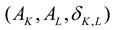 represents the three-dimensional coordinate point formed by the Kth and Lth meta-oscillators. are calculated via Eqs. (S6) and (S7). At the disturbance duration
 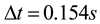 , all coordinate points clustered near the boundary (cyan). At
 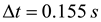 , three coordinate points [
 ,
,  , and
, and 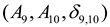 ] deviated outside the boundary, whereas the others remained clustered near it (magenta). The position of the point relative to the boundary directly determines the synchronization state.
represents the three-dimensional coordinate point formed by the Kth and Lth meta-oscillators. are calculated via Eqs. (S6) and (S7). At the disturbance duration , all coordinate points clustered near the boundary (cyan). At , three coordinate points [, , and ] deviated outside the boundary, whereas the others remained clustered near it (magenta). The position of the point relative to the boundary directly determines the synchronization state.(c). Real-time determination of synchronization admissibility. Observe the trajectory of in (b) separately. The temporal trajectory of coordinate point is shown for the unstable case (). The calculation range was  . Each cyan point represents the mean position of for a period of 1 second. The time T and the time interval
  are defined in Eq. (S8). The trajectory crossed the admissibility boundary outwardly [(7 s, 8 s)], preceding a rapid increase in the angle difference [(9 s,10 s)]. The outward crossing of a trajectory across the boundary indicates the onset of synchronization loss.
in (b) separately. The temporal trajectory of coordinate point is shown for the unstable case (). The calculation range was . Each cyan point represents the mean position of for a period of 1 second. The time T and the time interval are defined in Eq. (S8). The trajectory crossed the admissibility boundary outwardly [(7 s, 8 s)], preceding a rapid increase in the angle difference [(9 s,10 s)]. The outward crossing of a trajectory across the boundary indicates the onset of synchronization loss. (d) and (e). Experimental validation of the admissibility ( and ). The horizontal axis represents the time. The vertical axis represents the value of  . The maximum value is represented by
  (magenta), and the minimum value is represented by
  (cyan). In the stable case (),
  , indicating sustained synchronization. In the unstable case (),
 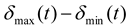 increased sharply after 9 s (
 ), confirming system desynchronization.
and ). The horizontal axis represents the time. The vertical axis represents the value of . The maximum value is represented by (magenta), and the minimum value is represented by (cyan). In the stable case (), , indicating sustained synchronization. In the unstable case (), increased sharply after 9 s (), confirming system desynchronization.(f). Experimental verification of partial synchronization. . Meta-oscillator 1 (cyan line) desynchronized after ~9 s, followed by meta-oscillators 2 (orange dashed line) and 10 (magenta line). Meta-oscillators 3–9 form a synchronized cluster (green lines). This pattern matches the cluster prediction from the spatial distribution in (b).
. Meta-oscillator 1 (cyan line) desynchronized after ~9 s, followed by meta-oscillators 2 (orange dashed line) and 10 (magenta line). Meta-oscillators 3–9 form a synchronized cluster (green lines). This pattern matches the cluster prediction from the spatial distribution in (b).First, we tested the ability of boundaries to distinguish between admissibility and inadmissibility. We increased the disturbance duration in small increments and observed the system's response. As shown in Figure 1b, a minute increase in disturbance duration from to , a mere 0.001 s, caused a dramatic shift in system behavior. Under admissible conditions (, cyan), all points clustered at the boundary, whereas at the inadmissible threshold (, magenta), specific points [,, and ] deviated outside it. The significant difference indicates that the boundary distinguishes between admissibility and inadmissibility. The correspondence between a point's position relative to the boundary and the synchronization was validated by time-domain simulations: The clustering of cyan points coincides with a bounded difference in  in Figure 1d, whereas the deviation of magenta points from the boundary indicates the large, growing desynchronization evident in Figure 1e. This consistency reveals the capability of the boundary to discriminate synchronization admissibility. To more thoroughly validate the discriminative capability of the boundary equation, we conducted systematic tests across all 39 nodes of the 10-oscillator system, generating a total of 78 distinct scenarios (39 admissible and 39 inadmissible cases, as detailed in Figure S2 and Table S1 in the supplemental material). In each scenario, the geometric criterion provided by Eq. (1) correctly matched the stability state (see S1 in the supplementary material) determined by time-domain simulations.
from to , a mere 0.001 s, caused a dramatic shift in system behavior. Under admissible conditions (, cyan), all points clustered at the boundary, whereas at the inadmissible threshold (, magenta), specific points [,, and ] deviated outside it. The significant difference indicates that the boundary distinguishes between admissibility and inadmissibility. The correspondence between a point's position relative to the boundary and the synchronization was validated by time-domain simulations: The clustering of cyan points coincides with a bounded difference in in Figure 1d, whereas the deviation of magenta points from the boundary indicates the large, growing desynchronization evident in Figure 1e. This consistency reveals the capability of the boundary to discriminate synchronization admissibility. To more thoroughly validate the discriminative capability of the boundary equation, we conducted systematic tests across all 39 nodes of the 10-oscillator system, generating a total of 78 distinct scenarios (39 admissible and 39 inadmissible cases, as detailed in Figure S2 and Table S1 in the supplemental material). In each scenario, the geometric criterion provided by Eq. (1) correctly matched the stability state (see S1 in the supplementary material) determined by time-domain simulations.Moreover, partial synchronization can also be diagnosed geometrically using the same criterion. As shown in Figure 1b, the positions of the 9 coordinate points reveal distinct synchronization clusters. Specifically, points ,, and residing outside the boundary indicate that the corresponding meta-oscillators (1st, 2nd, and 10th, respectively) lost synchronization admissibility. This result effectively divided the system into four synchronization groups: three desynchronized individual units (1st, 2nd and 10th) and one synchronized cluster comprising meta-oscillators 3–9. The time-domain results in Figure 1f are consistent with this diagnosis, confirming the manifestation of cluster synchronization16. Our approach thus offers a geometric interpretation for this phenomenon: Cluster synchronization arises from the localized loss of synchronization admissibility between oscillators when their representative coordinate points lie outside the boundary. This result, which simplifies the interpretation of partial synchronization15,17, was further corroborated by additional data (Table S1 in the supplemental material).
,, and residing outside the boundary indicate that the corresponding meta-oscillators (1st, 2nd, and 10th, respectively) lost synchronization admissibility. This result effectively divided the system into four synchronization groups: three desynchronized individual units (1st, 2nd and 10th) and one synchronized cluster comprising meta-oscillators 3–9. The time-domain results in Figure 1f are consistent with this diagnosis, confirming the manifestation of cluster synchronization16. Our approach thus offers a geometric interpretation for this phenomenon: Cluster synchronization arises from the localized loss of synchronization admissibility between oscillators when their representative coordinate points lie outside the boundary. This result, which simplifies the interpretation of partial synchronization15,17, was further corroborated by additional data (Table S1 in the supplemental material).Typically, we need to not only know whether a system is ultimately admissible, but also obtain this knowledge in real time. The timing of cluster splitting is well-suited for such real-time verification, as it involves multiple degrees of freedom, nonlinear transients, and multiple time scales18–21. The real-time transition of the system from admissibility to inadmissibility is shown in Figure 1c, where the coordinate point crossed the boundary outwardly during the time interval (8 s,9 s). This event is the direct precursor to the subsequent physical response: A dramatic increase in the angle difference  during (9 s,10 s). This finding indicates that the desynchronization is caused by crossing the boundary. The results of the time series in Figure 1e confirm that (9 s,10 s) marked the beginning of the loss of admissibility. This consistency indicates that the boundary is valid. This finding also demonstrates the capability of the boundary to distinguish complex admissibility phenomena in multiple oscillators11.
crossed the boundary outwardly during the time interval (8 s,9 s). This event is the direct precursor to the subsequent physical response: A dramatic increase in the angle difference during (9 s,10 s). This finding indicates that the desynchronization is caused by crossing the boundary. The results of the time series in Figure 1e confirm that (9 s,10 s) marked the beginning of the loss of admissibility. This consistency indicates that the boundary is valid. This finding also demonstrates the capability of the boundary to distinguish complex admissibility phenomena in multiple oscillators11.Furthermore, the result in Figure 1c that changes in amplitude precede increases in the angular difference during the loss of admissibility indicates that amplitude plays an indispensable role in determining admissibility. Therefore, while neglecting amplitude dynamics can effectively simplify the analysis22, incorporating it was essential for revealing the admissibility boundary reported here.
The synergy between the long-term assessment in Figure 1b and the short-term prediction in Figure 1c shows that the same surface governs admissibility across different time scales. The surface also explains the cluster synchronization phenomena (Figure 1f). These three independent finding convert to validate Eq. (1) as the visual representation of the synchronization admissibility boundary.
The same analysis as applied in Figure 1 was applied to another test system (3-oscillator). A strong external disturbance occurred at the node 4.
(a). Synchronization stabilization discrimination and partial synchronization. Two coordinate points clustered at the boundary when stable ( , cyan dots). was outside the boundary and away from when unstable (
 , magenta dots).
, cyan dots). was outside the boundary and away from when unstable (, magenta dots).(b). The real-time transition in admissibility for multiple oscillators. . Mirroring the dynamics in Figure 1c, crossed the boundary outwardly in the time interval (2 s, 3 s), and rapidly increased in the time interval (4 s, 5 s). These findings are in good agreement with the results presented in Figure 2d.
. Mirroring the dynamics in Figure 1c, crossed the boundary outwardly in the time interval (2 s, 3 s), and rapidly increased in the time interval (4 s, 5 s). These findings are in good agreement with the results presented in Figure 2d.(c) and (d) show the experimental validation of the synchronization admissibility and the real-time transition in admissibility for multiple oscillators. The time-series data corroborate the state predictions in (a), showing maintained synchrony at ( ) and loss of synchrony at (
 ).
).
() and loss of synchrony at ().(e). The phenomenon of partial synchronization. . After approximately 4 s, the system split into two synchronized clusters. Meta-oscillator 1 disengaged from the cluster (black line). Meta-oscillators 2 and 3 formed a synchronized cluster (red line and blue line).
. After approximately 4 s, the system split into two synchronized clusters. Meta-oscillator 1 disengaged from the cluster (black line). Meta-oscillators 2 and 3 formed a synchronized cluster (red line and blue line).Next, we verified that the boundary is independent of the structure. We repeated the verification experiment on a 3-oscillator system, and the results are shown in Figure 2. The 3-oscillator system differed significantly from the 10-oscillator system (used in Figure 1) in terms of scale, topology, and system parameters (see S2.2 in the supplementary material).
The three independent pieces of evidence shown in Figure 1 are reproduced exactly in Figure 2. First, by comparison with Figure 2c and d, we observed that the results in Figure 2a replicate the validity of the distinction between admissibility and inadmissibility shown in Figure 1b. Second, the results in Figure 2a also replicate the analysis of cluster synchronization shown in Figure 1b, as confirmed by the results in Figure 2e. Third, the results in Figure 2b replicate the real-time admissibility classification shown in Figure 1c, which is precisely confirmed by the results in Figure 2d. Together, these findings provide robust, multiscenario evidence that role of the boundary as an admissibility criterion is an inherent property, which is independent of the structure. This evidence stands in stark contrast to current understanding4,6,9,10.
Looking back at our validation, to rigorously test the validity of the boundary, we employed heterogeneous networks and introduced strong disturbances. Strong disturbances are typically accompanied by high uncertainty and can lead to strong nonlinear responses. These measures correspond to complex real-world scenarios. Our validation results demonstrate that the core functionalities of the boundary remained intact, even when dealing with these complex scenarios. These functionalities include real-time determination of admissibility for multioscillator systems and diagnosis of partial synchronization.
The fact that the same boundary equation is applicable to systems with different structures not only confirms that Eq. (1) is a validly applicable criterion, but also provides preliminary support for an inference: that the synchronization admissibility boundary is a potentially universal property that transcends any specific structure and has a more fundamental origin. This origin is precisely the real-number constraint that we will reveal in our “interpretation”.
Interpretation:
While extensive numerical validation across diverse networks demonstrates the robustness of Eq. (1), empirical evidence alone, no matter how extensive, cannot reveal why this boundary exists. To uncover the underlying principle, we must look beyond the data to the foundational assumptions of physics itself.
The validity of Eq. (1) across fundamentally different systems indicates a deeper insight: it may stem from a more fundamental physical origin than structure. This origin is ultimately rooted in a cornerstone of physics: For measurable physical quantities, their measured values must be real numbers. This cornerstone is a foundational premise of physics, prior to and independent of any assumptions about the type of oscillator or the structure of the interactions. Therefore, the angular frequency  of any oscillator is a real number. The common angular frequency emerges from the frequencies of these oscillators. That is, when
 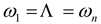 , we obtain
  . Thus, for any physically realizable synchronous state in oscillator systems, the common angular frequency must be a real number. This is the real number constraint, a direct corollary of that cornerstone. It is a tacit assumption so fundamental that it is never questioned in physical measurements. However, this seemingly trivial requirement, when applied to the synchrony boundary, has profound consequences: It imposes a condition on the relationship between oscillator amplitudes and frequencies.
of any oscillator is a real number. The common angular frequency emerges from the frequencies of these oscillators. That is, when , we obtain . Thus, for any physically realizable synchronous state in oscillator systems, the common angular frequency must be a real number. This is the real number constraint, a direct corollary of that cornerstone. It is a tacit assumption so fundamental that it is never questioned in physical measurements. However, this seemingly trivial requirement, when applied to the synchrony boundary, has profound consequences: It imposes a condition on the relationship between oscillator amplitudes and frequencies.Applying this constraint to Eq. (1) yields Eq. (2) (see S3.1 in the supplementary material for details). Starting from Eq. (1) and treating the common angular frequency (before disturbance), the real number constraint requires that the resulting quadratic equation in must have real roots (Eq. (S12)):
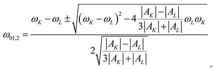
(before disturbance), the real number constraint requires that the resulting quadratic equation in must have real roots (Eq. (S12)):
This requirement yields a discriminant condition  , and its boundary
  simplifies to an equation containing no , an algebraic criterion depending only on observable states:
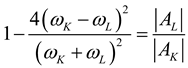 Where
Where  . Eq. (2) defines the exact mathematical boundary for the existence of a real synchronous angular frequency, thereby defining the condition for the existence of synchronization itself between the pair of oscillators K, L. Remarkably, it depends only on the oscillator states
  , confirming its independence from network topology or coupling parameters. In fact, Eq. (2) is mathematically equivalent to the real number constraint (see S3.1 in the supplementary material). This equivalence explains our initial question: critical points are so unique because they correspond to boundary between real and complex numbers.
, and its boundary simplifies to an equation containing no , an algebraic criterion depending only on observable states:
. Eq. (2) defines the exact mathematical boundary for the existence of a real synchronous angular frequency, thereby defining the condition for the existence of synchronization itself between the pair of oscillators K, L. Remarkably, it depends only on the oscillator states , confirming its independence from network topology or coupling parameters. In fact, Eq. (2) is mathematically equivalent to the real number constraint (see S3.1 in the supplementary material). This equivalence explains our initial question: critical points are so unique because they correspond to boundary between real and complex numbers.Upon further scrutiny (see S3.2 in the supplementary material), we found that Eq. (1) is an approximation. The exact boundary equation is shown below:

Unlike Eq. (1), is defined as 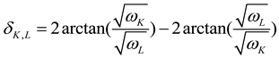 . Although Eq. (1) is an approximation, the discovery and validation sections of this paper follow the true sequence of scientific inquiry: we first identified this concise form of Eq. (1) from the data and then conducted all validation experiments based on it. To preserve the authentic narrative sequence of scientific discovery and maintain consistency in the visual analysis throughout the main text, we continue to use Eq. (1) in the discovery and validation sections. We provide a direct comparison of the results from Eqs. (1) and (3) (Figure S3 in the supplemental material), demonstrating that Eq. (1) is a reliable and valid approximate expression. Therefore, the core conclusions of this paper are not affected by this approximation.
is defined as . Although Eq. (1) is an approximation, the discovery and validation sections of this paper follow the true sequence of scientific inquiry: we first identified this concise form of Eq. (1) from the data and then conducted all validation experiments based on it. To preserve the authentic narrative sequence of scientific discovery and maintain consistency in the visual analysis throughout the main text, we continue to use Eq. (1) in the discovery and validation sections. We provide a direct comparison of the results from Eqs. (1) and (3) (Figure S3 in the supplemental material), demonstrating that Eq. (1) is a reliable and valid approximate expression. Therefore, the core conclusions of this paper are not affected by this approximation. Eq. (2) and Eq. (3) are mathematically equivalent (see S3.2 in the supplementary material): Eq. (3) is a parametric projection of Eq. (2) onto the observable state space via the real number 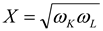 . The equivalence between Eq. (2) and Eq. (3), together with the equivalence between Eq. (2) and the real number constraint, establishes the equivalence: the synchronization admissibility boundary is an equivalent representation of the real number constraint. Thus, our interpretation reveals a profound fact: When applied to the synchronization of coupled oscillators, the requirement that physical quantities be real numbers emerges as the synchronization admissibility boundary. This key function is ultimately rooted in a cornerstone of physics.
. The equivalence between Eq. (2) and Eq. (3), together with the equivalence between Eq. (2) and the real number constraint, establishes the equivalence: the synchronization admissibility boundary is an equivalent representation of the real number constraint. Thus, our interpretation reveals a profound fact: When applied to the synchronization of coupled oscillators, the requirement that physical quantities be real numbers emerges as the synchronization admissibility boundary. This key function is ultimately rooted in a cornerstone of physics.Spontaneous synchronization layer near the boundary
The preceding discussion has established the synchronization admissibility boundary as a state-based, structure-independent criterion. Having defined this boundary, we now turn to investigating how it influences system behavior: Does the presence of the boundary affect the space near it? To answer this question, we examine the system's response as it approaches the boundary. We observed that the system’s behavior undergoes a marked change near the boundary. Our findings reveal a remarkable and robust emergent structure: a spontaneous synchronization layer. This phenomenon is not an isolated discovery but an attendant signature of the boundary itself. It provides direct evidence of self-organizing emergent phenomena at the limit defined by the real-number constraint.
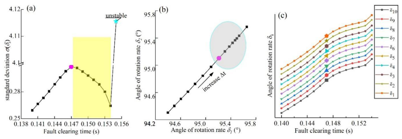
The disturbance duration increased from 0.140 s to 0.155 s. A strong external disturbance occurred at the node 18. .
increased from 0.140 s to 0.155 s. A strong external disturbance occurred at the node 18. . (a). Spontaneous synchronization of metaoscillators. The horizontal axis represents the disturbance duration. The vertical axis represents the standard deviation of  . The yellow area indicates the thin layer where spontaneous synchronization occurs. Here, the standard deviation
  began to decrease at 0.147 s (magenta) and increased by 1300% at 0.155 s (cyan) when the system was unstable. can be calculated via Eq. (S9).
. The yellow area indicates the thin layer where spontaneous synchronization occurs. Here, the standard deviation began to decrease at 0.147 s (magenta) and increased by 1300% at 0.155 s (cyan) when the system was unstable. can be calculated via Eq. (S9). (b). Phenomenon of the bottleneck. increased from 0.140 s to 0.154 s. The black arrow indicates the direction in which increased. From 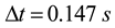 (the magenta dots) onward, the distance between neighboring points decreased in the direction of the black arrow (elliptical shaded area).
increased from 0.140 s to 0.154 s. The black arrow indicates the direction in which increased. From (the magenta dots) onward, the distance between neighboring points decreased in the direction of the black arrow (elliptical shaded area). (c). Starting points of spontaneous synchronization. The horizontal axis represents the disturbance duration. The amplified points indicate the starting points of spontaneous synchronization. All the starting points appeared at . The trends of all were almost identical. Combining (b) and (c) reveals that in this case, the structures in (b) exist between any two meta-oscillators. To clearly present the trend of , the linear scale on the vertical axis has been omitted; the corresponding data can be found in Table S2 in the supplemental material.
. The trends of all were almost identical. Combining (b) and (c) reveals that in this case, the structures in (b) exist between any two meta-oscillators. To clearly present the trend of , the linear scale on the vertical axis has been omitted; the corresponding data can be found in Table S2 in the supplemental material.We report a phenomenon of spontaneous synchronization that occurs as the system approaches the admissibility boundary. This phenomenon is evidenced by a decrease in the standard deviation (Figure 3a), indicating that the subsystems are spontaneously evolving toward a common angular frequency (not necessarily the one prior to disturbance). This evolution is a hallmark of spontaneous synchronization. However, this evolution does not restore the system to the complete synchronous state. Crucially, this self-organization is confined to a thin layer (yellow region in Figure 3a) immediately preceding the eventual loss of admissibility at . This geometric region may reflect collective self-organization near the admissibility threshold23. The phenomenon of spontaneous synchronization has been observed across different disturbance sites (Figure S4 in the supplemental material) and in distinct test systems (Figure S5 in the supplemental material), confirming its universality as an intrinsic characteristic of systems approaching the admissibility boundary. Furthermore, the reduction in the value of value within the thin layer reveals a change in the system's symmetry. If the system's state was merely a single-valued function of the control parameter , then its forward and backward variations should follow identical trajectories. The observed reduction in directly breaks this directional symmetry: During backward variation, the system cannot retrace the non-monotonic process of “first decreasing and then increasing” seen in the forward path because an increase in contradicts the definition of “synchronization” when a disordered state evolves into an ordered state. Consequently, the system state depends not only on but also on the manner in which the critical point is approached.
(Figure 3a), indicating that the subsystems are spontaneously evolving toward a common angular frequency (not necessarily the one prior to disturbance). This evolution is a hallmark of spontaneous synchronization. However, this evolution does not restore the system to the complete synchronous state. Crucially, this self-organization is confined to a thin layer (yellow region in Figure 3a) immediately preceding the eventual loss of admissibility at . This geometric region may reflect collective self-organization near the admissibility threshold23. The phenomenon of spontaneous synchronization has been observed across different disturbance sites (Figure S4 in the supplemental material) and in distinct test systems (Figure S5 in the supplemental material), confirming its universality as an intrinsic characteristic of systems approaching the admissibility boundary. Furthermore, the reduction in the value of value within the thin layer reveals a change in the system's symmetry. If the system's state was merely a single-valued function of the control parameter , then its forward and backward variations should follow identical trajectories. The observed reduction in directly breaks this directional symmetry: During backward variation, the system cannot retrace the non-monotonic process of “first decreasing and then increasing” seen in the forward path because an increase in contradicts the definition of “synchronization” when a disordered state evolves into an ordered state. Consequently, the system state depends not only on but also on the manner in which the critical point is approached.The system's trajectory in state space reveals a unique structural signature, a ‘bottleneck’, that, to our knowledge, has not been previously reported. For a constant step size , the distance between successive states decreases within the shaded area of Figure 3b, forming this bottleneck structure that exhibits a collective slowing-down. This spatial manifestation of deceleration emerges precisely at the temporal onset of spontaneous synchronization, i.e., when begins to decrease at (the magenta dots correspond exactly to in Figure 3b). A comparison between Figure 3b and S6a in the supplemental material confirms that this bottleneck structure is not a misleading result introduced by Eq. (S4), as it is also present in the oscillator's dynamic data. We hypothesize that the formation of a “bottleneck” may be related to emergent long-range coherence near critical points. In our visualization, this coherence coincides with trajectory clustering and deceleration (Figure 3b).
, the distance between successive states decreases within the shaded area of Figure 3b, forming this bottleneck structure that exhibits a collective slowing-down. This spatial manifestation of deceleration emerges precisely at the temporal onset of spontaneous synchronization, i.e., when begins to decrease at (the magenta dots correspond exactly to in Figure 3b). A comparison between Figure 3b and S6a in the supplemental material confirms that this bottleneck structure is not a misleading result introduced by Eq. (S4), as it is also present in the oscillator's dynamic data. We hypothesize that the formation of a “bottleneck” may be related to emergent long-range coherence near critical points. In our visualization, this coherence coincides with trajectory clustering and deceleration (Figure 3b). An accurate timeline of spontaneous synchronization is delineated by a distinct transition in the indicator  . As shown in Figure 3(c), the value of for all meta-oscillators undergoes a simultaneous and coherent shift at (amplified points). This timing coincides exactly with the moment when the standard deviation begins to decrease in Figure 3a, unambiguously linking the reversal in to the onset of spontaneous synchronization. Prior to this moment, remains positive; immediately afterward, becomes negative and remains so. This system-wide reversal indicates that marks the starting point of the spontaneous synchronization stage. The stage end is clearly indicated by the system's loss of synchronization at , a state change that is demonstrated by a dramatic increase in the standard deviation in Figure 3a and the corresponding time-domain simulation results in Figure 1e. Thus, the layer of spontaneous synchronization is bounded between and .
. As shown in Figure 3(c), the value of for all meta-oscillators undergoes a simultaneous and coherent shift at (amplified points). This timing coincides exactly with the moment when the standard deviation begins to decrease in Figure 3a, unambiguously linking the reversal in to the onset of spontaneous synchronization. Prior to this moment, remains positive; immediately afterward, becomes negative and remains so. This system-wide reversal indicates that marks the starting point of the spontaneous synchronization stage. The stage end is clearly indicated by the system's loss of synchronization at , a state change that is demonstrated by a dramatic increase in the standard deviation in Figure 3a and the corresponding time-domain simulation results in Figure 1e. Thus, the layer of spontaneous synchronization is bounded between and . The phenomena we report, including directional symmetry breaking and bottleneck structures, indicate collective, system-wide coordination mechanisms that emerge near the admissibility boundary. Near its admissibility critical points, the oscillator system exhibits emergent collective behaviors, which could make it a potential platform for exploring emergent collective dynamics in coupled systems2.
This newly identified spontaneous synchronization constitutes a distinct phenomenon, separate from those previously reported in power grids24. Existing phenomena typically describe how systems self-organize into synchronized states. In contrast, the novel spontaneous synchronization is uniquely characterized by its occurrence during a forward, disturbance-driven process toward inadmissibility and its association with the novel “bottleneck” structure. Moreover, its emergence is confined to the immediate vicinity of the synchronization admissibility boundary, as evidenced by experimental results under multiple disturbance scenarios (Figure 3a and S4 in the supplemental material). The intimate link between spontaneous synchronization and the admissibility boundary has a profound effect: The emergent layer of spontaneous synchronization is independent of the structure. More specifically, this independence is invariant across different structures: Throughout spontaneous synchronization, the coordinate point consistently resides near the boundary in the 3D coordinate system 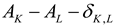 . More direct evidence comes from experiments using a separate test system (3-oscillator), where the phenomenon was also observed (Figure S5a in the supplemental material). Our observations provide direct evidence for a type of structure-independent spontaneous synchronization. First, the fact that spontaneous synchronization is independent of structure and occurs only near the boundary supports the view that the boundary is independent of structure. Second, spontaneous synchronization itself is a dynamic phenomenon, and the location where it emerges in state space is typically considered to be determined by structure, thus serving as an example of the “structure determines function” view4. However, our observations contradict this view and support the independence of the boundary. Moreover, the co-emergence of spontaneous synchronization and the boundary may suggest an intrinsic and close connection between emergent critical phenomena and admissibility conditions.
consistently resides near the boundary in the 3D coordinate system . More direct evidence comes from experiments using a separate test system (3-oscillator), where the phenomenon was also observed (Figure S5a in the supplemental material). Our observations provide direct evidence for a type of structure-independent spontaneous synchronization. First, the fact that spontaneous synchronization is independent of structure and occurs only near the boundary supports the view that the boundary is independent of structure. Second, spontaneous synchronization itself is a dynamic phenomenon, and the location where it emerges in state space is typically considered to be determined by structure, thus serving as an example of the “structure determines function” view4. However, our observations contradict this view and support the independence of the boundary. Moreover, the co-emergence of spontaneous synchronization and the boundary may suggest an intrinsic and close connection between emergent critical phenomena and admissibility conditions.In the case of the “bottleneck” phenomenon, the first derivative  of the the disturbed trajectory is continuous (see Figure 3c). Moreover, we observed a different phenomenon that occurred more frequently near the onset of spontaneous synchronization. The slope
  abruptly changes from greater than 1 to less than 1, causing the curve in Figure 3b to kink. is defined by
  . As shown in Figure 3b, when the state is admissible, and satisfy a relationship of the form
 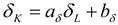 . Thus,
  . Owing to the monotonicity of
  with respect to , i.e.,
  . Therefore,
  and
and  occur simultaneously (see Figure S5b,c in the supplemental material). These results reveal the complexity of spontaneous synchronization.
of the the disturbed trajectory is continuous (see Figure 3c). Moreover, we observed a different phenomenon that occurred more frequently near the onset of spontaneous synchronization. The slope abruptly changes from greater than 1 to less than 1, causing the curve in Figure 3b to kink. is defined by . As shown in Figure 3b, when the state is admissible, and satisfy a relationship of the form . Thus, . Owing to the monotonicity of with respect to , i.e., . Therefore, and occur simultaneously (see Figure S5b,c in the supplemental material). These results reveal the complexity of spontaneous synchronization.The diversity of behaviors near the admissibility boundary and the varying thickness of spontaneously synchronized layers, highlight the following question: How can we understand the specific dynamic mechanisms underlying this spontaneous synchronization? Resolving these questions will be a primary objective of our future research.
Conclusion
In summary, this work demonstrates that the synchronization admissibility of coupled oscillator networks is governed by an intrinsic, structure-independent constraint: the real-number constraint. Mathematically, this constraint is equivalent to Eq. (1). This equivalence establishes that the synchronous admissibility boundary, the key function, emerges from a cornerstone of physics. By bypassing the reliance on network structure and parameters, the framework, which is grounded in the real number constraint can judge admissibility directly from state measurements. This framework broadens the scope of synchrony analysis beyond specific structures. It provides a principle-based analytical framework for oscillator systems characterized by strong nonlinearity, high heterogeneity, uncertainty, and unknown or time-varying structures—systems where traditional structure-dependent methods face severe challenges. These findings suggest that, at least when synchronization limits are being assessed, the focus can shift from accurate structure modeling to the analysis of observable collective dynamics, opening a new approach for systems with abundant data but incomplete structural information. It thus offers a simplified approach to analyzing admissibility in complex systems. Finally, we report a novel spontaneous synchronization layer near this boundary whose features suggest underlying critical phenomena.
The independence of this boundary from structure is not an empirical coincidence, but a mathematical consequence of a cornerstone of physics—one that is logically prior to any specific structure. This work thus provides a counterexample to the “structure determines function” that understanding function requires an understanding of structure. The discovery of a structure-independent boundary indicates that certain functions may emerge directly from principles that exist a priori and transcend structure. By demonstrating a key function that traces directly to a fundamental physical principle, this work provides concrete instances and practical methods for the “principle emerges function.”
Although we have identified the boundary equation and proved its equivalence to the real-number constraint, deriving the same result from the detailed network structure and microscopic dynamics remains a challenging task. This difficulty may reflect a gap between emergent phenomena and structural details8. In addition to the power system described in this paper, due to the fact that “measurable quantities must be real” is a fundamental constraint governing all natural sciences, and the equation is mathematically equivalent to this constraint, it may, in principle, be applicable to other discipline involving synchronization phenomena—such as neuronal synchronization in neuroscience, or chemical and biological oscillator networks. Further research also includes extensions time-delay scenarios, noise-dominated scenarios, and the corollary (S4 in the supplemental material). These issues are a central direction for future research.
Finally, this line of inquiry, in turn, leads us to more profound questions: Do other features, similarly independent of structure, exist in complex systems? If so, what is their physical origin? In addition, could their existence imply an underlying, unified description of complex systems? Although the resulting equations may vary depending on the field or problem, these subsequent studies are likely to construct an understanding system of emergence.
Methods
This study validated the proposed method using two standard and significantly distinct power grid test systems, namely, the 3-oscillator system25 (Figure 2, Figures S3 and S5) and the 10-oscillator system26 (Figure 1, Figure 3, Figures S2–S4, S6, and S7 and Table S1). Standard power flow calculations and transient stability calculations were performed in the above network model using the PSASP toolbox27.
was set to 314.16 rad/s. All external control mechanisms were turned off. We calculated the angular frequency and the terminal amplitude of the ith oscillator for various disturbance durations over a time window T of 20 seconds, starting from disturbance inception. The disturbance scenario (the site, the type, and the duration ) was defined. We set all the disturbances as three-phase short circuits to ground. The simulation process was repeated until the system transitioned from a stable state to a loss of synchronization state, as confirmed by the simulation results.Supplementary Materials
The following supporting information can be downloaded at the website of this paper posted on Preprints.org.
Data Availability
All the data that support the findings of this study are available at https://doi.org/10.57760/sciencedb.24825.
References
- Ye, Z.; Wu, Y.; Ding, Q.; et al. Finding synchronization state of higher-order motif networks by dynamic learning. Physical Review Research 2024, 6. [Google Scholar] [CrossRef]
- Koronovskii, A. A.; Moskalenko, O. I.; Hramov, A. E. synchronization in complex networks. Technical Physics Letters 2012, 38, 924–927. [Google Scholar] [CrossRef]
- Dörfler, F.; Bullo, F. Synchronization in complex networks of phase oscillators: A survey. Automatica 2014, 50, 1539–1564. [Google Scholar] [CrossRef]
- Newman, M. E. J. The structure and function of complex networks. SIAM Review 2003, 45, 167–256. [Google Scholar] [CrossRef]
- Pecora, L. M.; Carroll, T. L. Master stability functions for synchronized coupled systems. Physical Review Letters 1998, 80, 2109–2112. [Google Scholar] [CrossRef]
- Millán, A. P.; Sun, H.; Giambagli, L.; et al. Topology shapes dynamics of higher-order networks. Nature Physics 2025, 21, 353–361. [Google Scholar] [CrossRef]
- Nazerian, A.; Hart, J. D.; Lodi, M.; et al. The efficiency of synchronization dynamics and the role of network syncreactivity. Nature Communications 2024, 15, 1–13. [Google Scholar] [CrossRef] [PubMed]
- Andersen, P. W. More is different. Science 1972, 177, 393–396. [Google Scholar] [CrossRef]
- Gallo, A.; Tian, Y.; Lambiotte, R.; et al. Global synchronization in Matrix-Weighted networks. Communications Physics 2025, 8, 1–13. [Google Scholar] [CrossRef]
- Lodi, M.; Panahi, S.; Sorrentino, F.; et al. Patterns of synchronized clusters in adaptive networks. Communications Physics 2024, 7. [Google Scholar] [CrossRef]
- Yang, S.; Li, B.; Hao, Z.; et al. Multi-Swing Transient Stability of Synchronous Generators and IBR Combined Generation Systems. IEEE Transactions on Power Systems 2025, 40, 1144–1147. [Google Scholar] [CrossRef]
- Dörfler, F.; Chertkov, M.; Bullo, F. Synchronization in complex oscillator networks and smart grids. Proceedings of the National Academy of Sciences of the United States of America 2013, 110, 2005–2010. [Google Scholar] [CrossRef]
- Scheffer, M.; Carpenter, S. R.; Lenton, T. M.; et al. Anticipating critical transitions. Science 2012, 338, 344–348. [Google Scholar] [CrossRef]
- Nishikawa, T.; Motter, A. E. Synchronization is optimal in nondiagonalizable networks. Physical Review E - Statistical, Nonlinear, and Soft Matter Physics 2006, 73, 1–4. [Google Scholar] [CrossRef]
- Sorrentino, F.; Pecora, L. M.; Hagerstrom, A. M.; et al. Complete characterization of the stability of cluster synchronization in complex dynamical networks. Science Advances 2016, 2, 1–8. [Google Scholar] [CrossRef]
- Cho, Y. S.; Nishikawa, T.; Motter, A. E. Stable Chimeras and Independently Synchronizable Clusters. Physical Review Letters 2017, 119. [Google Scholar] [CrossRef]
- Lück, S.; Pikovsky, A. Dynamics of multi-frequency oscillator ensembles with resonant coupling. Physics Letters, Section A: General, Atomic and Solid State Physics 2011, 375, 2714–2719. [Google Scholar] [CrossRef]
- Guckenheimer, J.; Holmes, P.; Slemrod, M. Nonlinear Oscillations Dynamical Systems, and Bifurcations of Vector Fields. Journal of Applied Mechanics 1984, 51, 947–947. [Google Scholar] [CrossRef]
- Xu, H. Finite-Time Stability Analysis: A Tutorial Survey. Complexity 2020: (2020).
- Ajala, O., Dominguez-Garcia, A., Sauer, P., et al. A Second-Order Synchronous Machine Model for Multi-swing Stability Analysis. 51st North American Power Symposium, NAPS 2019 (2019).
- Omel’chenko, O. E. Periodic orbits in the Ott-Antonsen manifold. Nonlinearity 2023, 36, 845–861. [Google Scholar] [CrossRef]
- Dörfler, F.; Bullo, F. Synchronization and transient stability in power networks and nonuniform Kuramoto oscillators. SIAM Journal on Control and Optimization 2012, 50, 1616–1642. [Google Scholar] [CrossRef]
- Gutiérrez, R.; Cuerno, R. Nonequilibrium criticality driven by Kardar-Parisi-Zhang fluctuations in the synchronization of oscillator lattices. Physical Review Research 2023, 5, 1–26. [Google Scholar] [CrossRef]
- Motter, A. E.; Myers, S. A.; Anghel, M.; et al. Spontaneous synchrony in power-grid networks. Nature Physics 2013, 9, 191–197. [Google Scholar] [CrossRef]
- Anderson, P. M. & Fouad, A. A. Power System Control and Stability. (John Wiley & Sons, 2008).
- Pai, A. Energy Function Analysis for Power System Stability. (Springer Science & Business Media, 1989).
- Wu Zhongxi & Zhou Xiaoxin. Power System Analysis Software Package (PSASP)-an integrated power system analysis tool. in POWERCON ’98. 1998 International Conference on Power System Technology. Proceedings (Cat. No.98EX151) 1: 7–11 (IEEE).
Figure 1.
Validity and accuracy of the synchronization admissibility boundary (meta-oscillators).
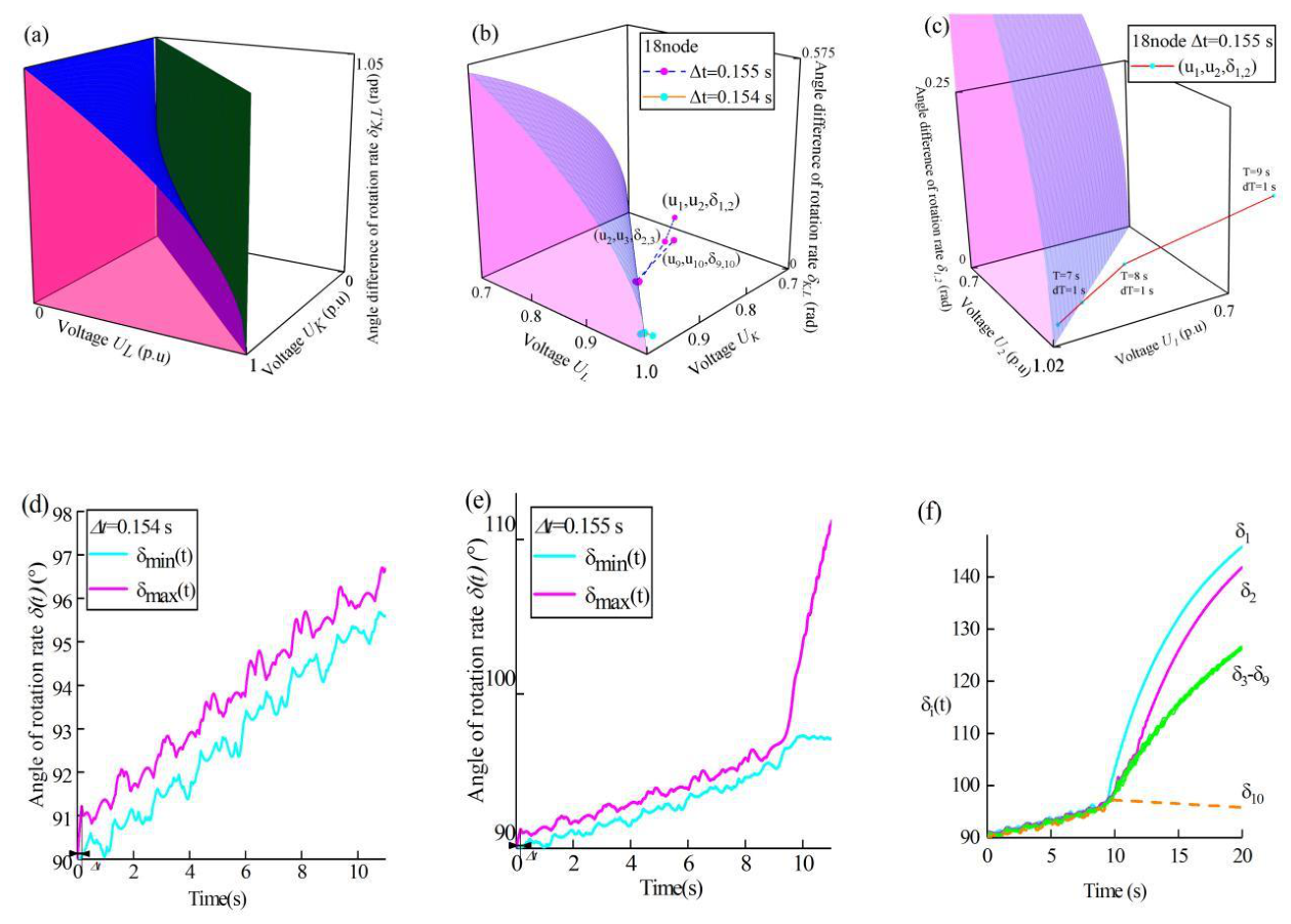
Figure 2.
Structure-independent synchronization admissibility boundary. (meta-oscillators).
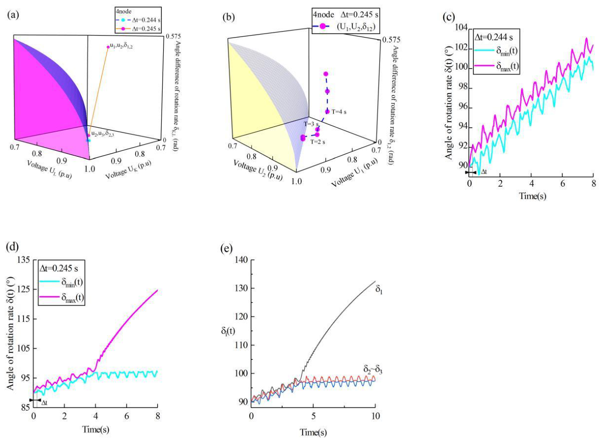
Figure 3.
Emergence of self-organization near the admissibility boundary. (meta-oscillators in the 10-oscillator).
Figure 3.
Emergence of self-organization near the admissibility boundary. (meta-oscillators in the 10-oscillator).
Disclaimer/Publisher’s Note: The statements, opinions and data contained in all publications are solely those of the individual author(s) and contributor(s) and not of MDPI and/or the editor(s). MDPI and/or the editor(s) disclaim responsibility for any injury to people or property resulting from any ideas, methods, instructions or products referred to in the content. |
© 2026 by the authors. Licensee MDPI, Basel, Switzerland. This article is an open access article distributed under the terms and conditions of the Creative Commons Attribution (CC BY) license (http://creativecommons.org/licenses/by/4.0/).
Copyright: This open access article is published under a Creative Commons CC BY 4.0 license, which permit the free download, distribution, and reuse, provided that the author and preprint are cited in any reuse.