Network-Independent Synchronous Stability Boundary and Spontaneous Synchronization

1. Introduction

Synchronization occurs when interconnected units—from fireflies to generators—adjust their rhythms to act in concert. This collective behavior is crucial for understanding the function of diverse complex systems [1]. Current research relies on a traditional framework to constructively understand synchronization. This framework posits that knowledge of the network architecture (e.g., the adjacency matrix) and each unit’s dynamics is a prerequisite for predicting collective outcomes [2,3].

This framework, however, faces some fundamental obstacles in real world systems: interactions are difficult to fully observe, structural data are incomplete, and exceedingly large networks lead to prohibitive computational costs [4,5,6]. These issues are compounded by higher-order interactions, nonlinear dynamics, and parametric uncertainties [7]. Power grids exhibit key complex network features and the dynamics of generators, described by the swing equation, is equivalent to the well-studied Kuramoto model [1,2]. Additionally, the very real world attributes of power grids, their vast scale, structural complexity, and dynamic nonlinearity, make them a domain where obtaining the requisite information is profoundly challenging. These factors make the power grid a suitable test bed for the synchronization of complex networks [8,9,10,11]. Currently, prevailing analytical methods for power systems have made significant progress, yet they remain constrained by these challenges [1,12,13,14,15,16]. Among these, two prominent strategies are the identification of the synchronous stability boundary, a cornerstone concept in grid stability defined as the union of critical points beyond which the system desynchronizes [15,17,18], and the study of spontaneous synchronization conditions, wherein systems self-organize without external guidance [2,16,19].

Here, we introduce a novel framework grounded in a principle (or consensus) regarding synchronization. This framework reveals that synchronous stability is governed by boundary. We derive and rigorously prove an elegant equation that universally describes this boundary for power systems. A pivotal insight is that this equation is independent of any specific network, providing a general criterion for stability. Here, the network encompasses both the network topology and the system parameters (e.g., line impedance, inertia constants and damping). To enable its application to multigenerator systems, we developed a novel and effective reduction method for higher-order interactions. This algorithm also holds potential for interdisciplinary applications. The validity of this boundary equation and the reduction algorithm is confirmed through mathematical proofs and simulation experiments.

This work also yielded other significant results. First, the boundary equation unifies the seemingly contradictory phenomena of symmetry and asymmetry, showing that both can enhance synchronization. Second, we identify a new type of spontaneous synchronization that emerges exclusively near the stability boundary and is therefore likewise independent of the network. Most significantly, these findings, particularly the network-independent nature of both the stability boundary and the associated spontaneous synchronization, challenge the structural basis of synchronization on complex networks. This framework provides a unified and powerful approach to studying synchronization amid real-world complexity and uncertainty, with conclusions that have direct implications for a wide range of disciplines.

Stability boundary

Synchronization emerges when the suppression (of the loss of synchrony) dominates the dissimilarity, a simple principle regarding synchronization from which we derive the synchronization stability boundary equation [2]. The system is synchronous and stable when the suppression term $P_{\Delta u}$, exceeds the dissimilarity term $P_{\partial u}$ and loses synchronization when $P_{\Delta u}<P_{\partial u}$. Consequently, the condition $P_{\Delta u}$=$P_{\partial u}$ defines the synchronous stability boundary, described by the following equation (see appendix B):

$$\left(\left|u_K\right|=\left|u_L\right|\right)\cup \left(\left|u_L\right|/\left|u_K\right|=2\cos {\delta }_{K,L}-1\right)$$

(1)

Strictly speaking, this equation defines the boundary of the physically admissible domain—that is, the set of all possible system states that comply with fundamental physical laws (see appendix D). In this paper, we interpret this physically admissible domain as representing the system’s synchronization stability region. This explanation is reasonable for two reasons: 1) physical existence is a prerequisite for stability; 2) for power systems, our experiments confirm that the two boundaries are indistinguishable in all tested scenarios.

In power systems, the voltages $\left|u_K\right|$ and $\left|u_L\right|$ of the Kth and the Lth generators, and the angle difference ${\delta }_{K,L}$ of their rotation rates (where ${\delta }_{K,L}=\left|{\delta }_K-{\delta }_L\right|\ge 0$) are considered. Here, the rotation rate of a generator is characterized by an angle of rotation rate (ARR) ${\delta }_K$ (not the phase angle), and synchronization corresponds to ${\delta }_1=\dots ={\delta }_K={\delta }_L=\dots ={\delta }_n$. The voltage has been previously overlooked for simplicity [16,20] but is crucial for the synchronization stability of the grid [refer to Figure 1(c)].

Eq. (1) actually defines the synchronous stability boundary for two generators. For multigenerators systems, since all boundary equations of pairs of generators share identical forms, the visualized graphs completely coincide, as shown in Figure 1(a).

The expression in Eq. (1) establishes a formal link between synchronous stability and “pairwise interactions.” It is crucial to note, however, that the interactions among generators are inherently higher order. Therefore, to enable stability analysis within this framework, our method employs a mathematical transformation (Eq. S2) that maps these higher-order interactions into pairwise interactions between meta-generators. The meta-generator is the direct result of this transformation, and its successful application (as detailed in Figure 1 and Figure 2) validates its functional equivalence to an effective reduction method. Unlike the generator system, for the Kth and the Lth meta-generator, L=K+1. Unlike the generator perspective (Figure S2), the meta-generator framework endows the “synchronization stability” relation with the property of an equivalence class. This crucial property thereby provides a rigorous foundation for analyzing synchronization stability at the subsystem level and for investigating phenomena such as partial synchronization (Figures 1(b) and 2(a)).

Critically, this transformation preserves synchronization stability (see appendix F), which ensures a strict equivalence in the stability states between the generator and meta-generator systems. This equivalence establishes a powerful validation framework: demonstrating that the stability boundary correctly classifies the meta-generators (Figure 1 and Figure 2) directly confirms its validity for the original generator system. This algorithm has no direct connection to specific physical scenarios, and therefore can be applied directly across different disciplines.

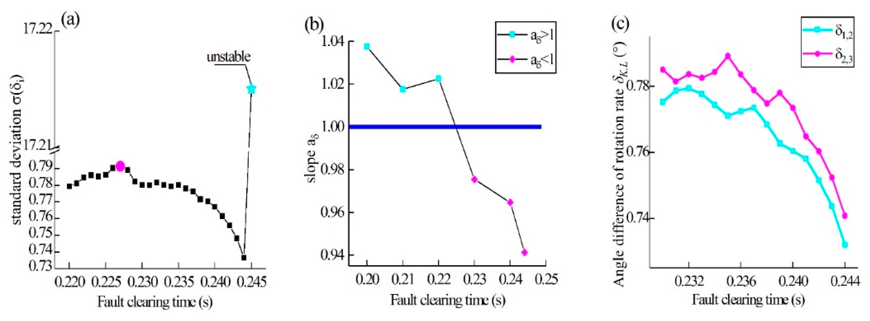
A New England test system was used. A three-phase short-circuit ground fault occurred at node 18. The data in Figure 1 are derived from numerical simulation experiments. $\Delta t$ represents the fault clearing time, and $d(\Delta t)=0.001s$ denotes the step length typically used in power system studies.

(a). Visualization of the stability boundary. The stability boundary in Eq. (1) (blue surface and dark green plane) and the pink planes $0-u_L-{\delta }_{K,L}$, $u_K-0-{\delta }_{K,L}$ and $u_K-u_L-0$ collectively define the boundaries and enclose the stability domain. The identical boundary form enables a unified stability assessment.

(b). Synchronization stability and partial synchronization. $(u_K,u_L,{\delta }_{K,L})$ represents the three-dimensional (3D) coordinate point formed by the Kth and Lth meta-generators. $(u_K,u_L,{\delta }_{K,L})$ are calculated via Eqs. (S3) and (S4). At fault clearing time $\Delta t=0.154s$, all coordinate points cluster near the boundary (cyan). At $\Delta t=0.155s$, three coordinate points [$(u_1,u_2,{\delta }_{1,2})$,$(u_2,u_3,{\delta }_{2,3})$, and $(u_9,u_{10},{\delta }_{9,10})$] deviate outside the boundary, whereas the others remain clustered near it (magenta). The position of the point relative to the boundary directly diagnoses the synchronization state.

(c). Tracking the onset of desynchronization. The temporal trajectory of coordinate point $\left(u_1,u_2,{\delta }_{1,2}\right)$ is shown for the unstable case ($\Delta t=0.155s$). The calculation range is $6s\le T\le 9s$. Each cyan point represents the mean position of $\left(u_1,u_2,{\delta }_{1,2}\right)$ for a period of 1 second. The time T and the time interval $dT=1s$ are defined in Eq. (S5). The trajectory crosses the stability boundary outwardly [(7 s, 8 s)], preceding a rapid increase in the angle difference ${\delta }_{K,L}$ [(9 s,10 s)]. The outward crossing of a trajectory across the boundary pinpoints the onset of synchronization loss.

(d) and (e). Experimental validation of the stability ($\Delta t=0.154s$ and $\Delta t=0.155s$). The horizontal axis represents the time. The vertical axis represents the value of ${\delta }_i(t)$. ${\delta }_i(t)$ are calculated with simulation software and Eq. (S2). The maximum value is represented by ${\delta }_{\max }(t)$ (magenta), and the minimum value is represented by ${\delta }_{\min }(t)$ (cyan). In the stable case ($\Delta t=0.154s$), ${\delta }_{\max }(t)-{\delta }_{\min }(t)\approx 1°$, indicating sustained synchronization. In the unstable case ($\Delta t=0.155s$), ${\delta }_{\max }(t)-{\delta }_{\min }(t)$ increases sharply after 9 s ($\approx 14°$), confirming system desynchronization.

(f). Experimental verification of partial synchronization. $\Delta t=0.155s$. Meta-generator 1 (cyan line) desynchronizes after ~9 s, followed by meta-generators 2 (orange dashed line) and 10 (magenta line). Meta-generators 3~9 form a synchronized cluster (green lines). This pattern matches the cluster prediction from the spatial distribution in (b).

Figure 1(a) visualizes Eq. (1) within a three-dimensional (3D) coordinate system. Geometrically, the surfaces defined by Eq. (1) are fixed, which provides an intuitive indication of its independence from network topology and system parameters. We now proceed to validate this conclusion experimentally. Three lines of evidence confirm that Eq. (1) universally describes the synchronization stability boundary: 1) it distinguishes stable from unstable states [see Figures 1(b) and 2(a)], 2) it captures the stability of multiple swings [see Figures 1(c) and 2(b)], and 3) it explains partial synchronization patterns [see Figures 1(f) and 2(e)].

The boundary equation provides a definitive geometric criterion for power system stability. For a system with n meta-generators, the state is represented by n-1 points in a 3D coordinate space. This representation reveals a powerful discriminative capability: as shown in Figure 1(b), a minute increase in fault clearing time $\Delta t$ from $\Delta t=0.154s$ to $\Delta t=0.155s$, a change of merely 0.001 s, causes a dramatic shift in system behavior. Under stable conditions ($\Delta t=0.154s$, cyan), all points cluster at the boundary, whereas at the instability threshold ($\Delta t=0.155s$, magenta), specific points ($(u_1,u_2,{\delta }_{1,2})$,$(u_2,u_3,{\delta }_{2,3})$, and $(u_9,u_{10},{\delta }_{9,10})$) deviate outside it. This spatial deviation is the direct geometric manifestation of the condition $P_{\Delta u}<P_{\partial u}$, signifying a loss of synchronization. The definitive correspondence between a point’s position relative to the boundary and the system’s physical state is rigorously validated by time-domain simulations: the clustering of cyan points coincides with a bounded difference in ${\delta }_K$ in Figure 1(d), whereas the deviation of points from the boundary predicts the large, growing desynchronization evident in Figure 1(e). The reproducibility of this exact discriminative function in the topologically distinct 3-generator system (Figure 2(a), (c) and (d)), along with analogous results under varied fault scenarios (Figure S5), provides robust, multiscenario evidence that the boundary’s role as a stability criterion is an inherent property, independent of the network topology or perturbation [2,21,22]. To thoroughly validate the universality of the boundary equation, we conducted tests on all 39 nodes of the New England test system (Table S1 for details). Across all 78 stable and unstable cases, Eq. (1) achieved discrimination with an accuracy of 100%.

Furthermore, Figure 1(b) provides a novel and direct geometric diagnosis of partial synchronization. The positions of the 9 coordinate points reveal distinct synchronization clusters. Specifically, points $(u_1,u_2,{\delta }_{1,2})$, $(u_2,u_3,{\delta }_{2,3})$, and $(u_9,u_{10},{\delta }_{9,10})$ residing outside the boundary indicate that the corresponding meta-generators (1st, 2nd, and 10th, respectively) have lost synchronization stability. This result effectively divides the system into four synchronization groups: three desynchronized individual units (1st, 2nd and 10th) and one synchronized cluster comprising meta-generators 3rd through 9th. The time-domain results in Figure 1(f) are in perfect agreement with this diagnosis, confirming the manifestation of cluster synchronization[23,24]. Our approach thus offers a unified geometric interpretation for this phenomenon: cluster synchronization arises from the localized loss of synchronization stability between oscillators when their representative coordinate points lie outside the universal boundary[25,26]. This mechanism, which improves our understanding of partial synchronization, is further corroborated by additional data (Table S1). Critically, this diagnostic framework is universally applicable in power systems, as demonstrated by the consistent combination of geometric diagnosis in Figure 2(a) and time-domain validation in Figure 2(e) for the completely different 3-generator systems.

Figure 1(C) captures the system’s transition from stability to instability, showing coordinate point $(u_1,u_2,{\delta }_{1,2})$ crossing the boundary outwardly during the time interval (8 s,9 s). This event is the direct precursor to the subsequent physical response: a dramatic increase in the angle difference ${\delta }_{1,2}$ during (9 s,10 s), which leads to the eventual loss of synchronization, as confirmed by the time-domain simulation in Figure 1(E). The consistent temporal sequence—boundary crossing preceding desynchronization—establishes that this crossing marks the real-time onset of synchronization loss. This demonstrates the boundary’s capacity as a dynamic predictor, capable of discriminating the complex phenomenon of multiswing stability for multiple generators[27,28]. Critically, this entire sequence of events, from boundary crossing to desynchronization, is replicated in the completely different 3-generator system (Figures 2(b) and (d)), underscoring universality of the predictive power across networks. Furthermore, the critical role of the voltage term in this predictive boundary suggests that the common assumption of disregarding voltage variations [8] may be inadequate when the system approaches the stability boundary, even for short-term dynamic studies. Ultimately, the synergy between the long-term stability assessment in Figure 1(b) and the short-term transient prediction in Figure 1(c) confirms that the same boundary equation governs stability across different time scales and operational scenarios. This coherence underpins a unified framework for synchronous stability analysis in power systems.

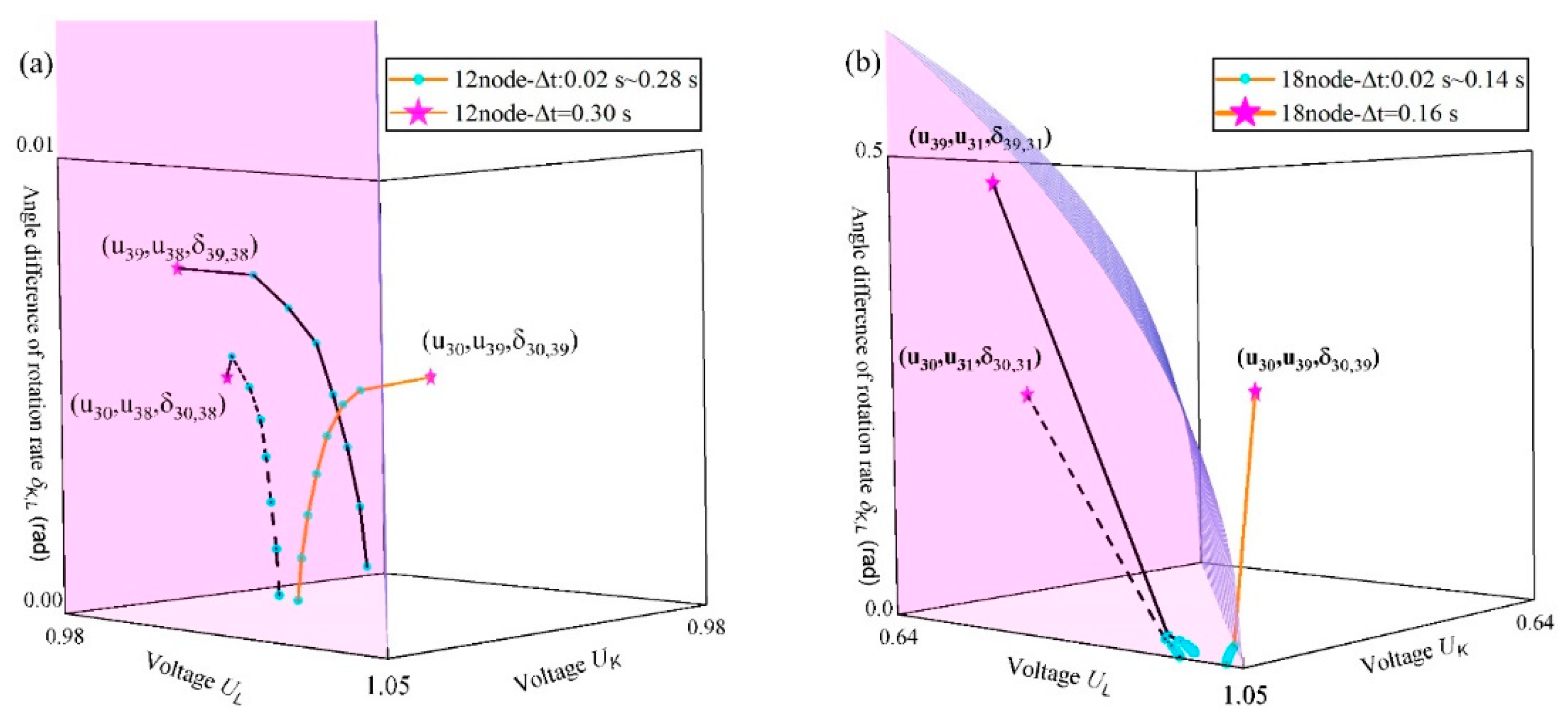
The same analysis as in Figure 1 is applied to the 3-generator system. A three-phase short circuit to a ground fault occurred at the 4-node.

(a). Synchronization stabilization discrimination and partial synchronization. Two coordinate points cluster at the boundary when stable ($\Delta t=0.244s$, cyan dots). $\left(u_1,u_2,{\delta }_{1,2}\right)$ is outside the boundary and away from $(u_2,u_3,{\delta }_{2,3})$ when unstable ($\Delta t=0.245s$, magenta dots).

(b). Stability of multiple swings for multiple generators. $\Delta t=0.245s$. Mirroring the dynamics in Figure 1(c), $\left(u_1,u_2,{\delta }_{1,2}\right)$ crosses the boundary outwardly in the time interval $\left(2s,3s\right)$, and ${\delta }_{1,2}$ rapidly increases in the time interval $\left(4s,5s\right)$. These findings are in good agreement with the results presented in Figure 2(d).

(c) and (d) show the experimental validation of the synchronous stability and the stability of multiple swings for multiple generators. The time-series data corroborate the state predictions in (a), showing maintained synchrony at $\Delta t=0.244s$ (${\delta }_{\max }(t)-{\delta }_{\min }(t)\approx 3°$) and loss of synchrony at $\Delta t=0.245s$ (${\delta }_{\max }(t)-{\delta }_{\min }(t)\approx 28°$).

(e). The phenomenon of partial synchronization. ($\Delta t=0.245s$). After approximately 4 s, the system splits into two synchronized clusters. Meta-generator 1 disengages from the cluster (black line). Meta-generators 2 and 3 form a synchronized cluster (red line and blue line).

The 10-generator New England system and the 3-generator system are two canonical test systems recognized as completely distinct in scale, topology, and system parameters, such as line impedance and generator inertia [29,30]. The successful replication of the boundary’s core functions, stability discrimination, multigenerator and multiswing instability prediction, and partial synchronization diagnosis, across these disparate systems provides a formidable foundation for a robust and universal conclusion. Together, this robust, multifaceted validation rigorously demonstrates the recognition that the synchronization stability boundary is independent of network topology, system parameters, and perturbation locations. We demonstrate that the emergence of the stability boundary, as a key function of the network, can be directly established on a simple principle rather than being governed by structural details. This independence between function and network challenges the structural foundations in complex networks [2,21,22]. This finding is further underpinned by rigorous mathematical proof which directly links the emergence of synchronization to the fundamental principle (see appendix D).

By bypassing reliance on network structure and parameters, this framework can judge stability directly from individual state measurements. It thus offers a radically simplified approach to analyzing stability in complex systems. It is particularly noteworthy that the boundary equation $\left|\partial u\right|/\left|\Delta u\right|=1$ was identified prior to its physical interpretation (Appendix B). This sequence of discovery suggests that the boundary may be rooted in an origin more fundamental than any specific disciplinary context. A key piece of evidence lies in the fact that the generator swing equation used in this work for independent validation is equivalent to the Kuramoto model [1,2]. This equivalence implies that our findings reveal a universal law applicable to all oscillator networks of the same type. Furthermore, the stability boundary derived in this paper, along with its network-independent nature, fundamentally defines the synchronous stability limits for a broad class of oscillator networks. Based on this, extending the “amplitude–frequency” framework (such as $u_i(t)$ and ${\delta }_i(t)$ in this work) established in this study to other disciplines such as biological rhythms and chemical oscillators has become a highly promising direction for future research [31,32,33].

This line of inquiry, in turn, leads us to more profound questions: Do other features, similarly independent of structure, exist in complex systems? If so, what is their physical origin? And could their existence imply an underlying, unified description of complex systems?. Seeking answers to these questions is precisely the crucial step toward a new cognitive landscape centered on emergence.

Important implications can be derived from the expression of Eq. (1). Specifically, the left-hand side of Eq. (1) represents the global stability domain [21] (i.e., when $\left|u_K\right|=\left|u_L\right|$,$\forall {\delta }_{K,L}\ge 0,P_{\Delta u}=P_{\partial u}$).

$$\left|u_K\right|=\left|u_L\right|$$

(2)

represents a manifestation of the symmetry of the system. Such symmetry typically originates from underlying topological symmetries in the network and the homogeneity of the oscillators. This finding explains why high symmetry can facilitate synchronization in complex networks and aligns with established understanding [34,35].

Conversely, the variant form of the right-hand side of Eq. (1) is as follows:

$${\delta }_{K,L}^{cr}=\arccos (1-{\displaystyle \frac{\left|u_K\right|-\left|u_L\right|}{2\left|u_K\right|}})$$

(3)

reveals that asymmetry can also enhance stability. Such asymmetry often stems from topological asymmetries or heterogeneity. Here, ${\delta }_{K,L}^{cr}$ represents the stability margin of the Kth and Lth meta-generator angle difference of the rotation rate; that is, for $(u_K,u_L,{\delta }_{K,L})$, the system remains synchronously stable when ${\delta }_{K,L}^{cr}>{\delta }_{K,L}$. When $\left|u_K\right|,\left|u_L\right|$ are sufficiently close [36], ${\delta }_{K,L}^{cr}$ tends to 0. Crucially, ${\delta }_{K,L}^{cr}$ increases with increasing voltage asymmetry $\left|u_K\right|-\left|u_L\right|$, indicating that the stability domain expands as the system becomes more asymmetric. This finding explains the recently observed synchronization facilitation phenomenon in highly asymmetric systems [37,38]. These findings suggest a practical advantage: because perfect symmetry is fragile under perturbation, designing for controlled asymmetry can be a preferable strategy for maintaining stability. When ${\delta }_{K,L}>{\displaystyle \frac{\pi }{3}}$, the Kth and Lth meta-generators are not synchronized. Thus, the range of the synchronous stability domain is finite under asymmetric conditions.

Consequently, both high symmetry and high asymmetry may promote synchronization. The expression of Eq. (1) is very simple, however, it harmonizes these two contradictory conclusions well and requires no prior analysis of the network structure.

Spontaneous synchronization in a power system

To understand how systems fail, it is equally important to investigate the behavior of a disturbed system at the stability boundary [39]. When perturbed and near this brink, the system’s trajectory, described by the polar coordinate variable ($u_i,{\delta }_i$) of the meta-generators, reveals a surprising structure indicative of spontaneous synchronization.

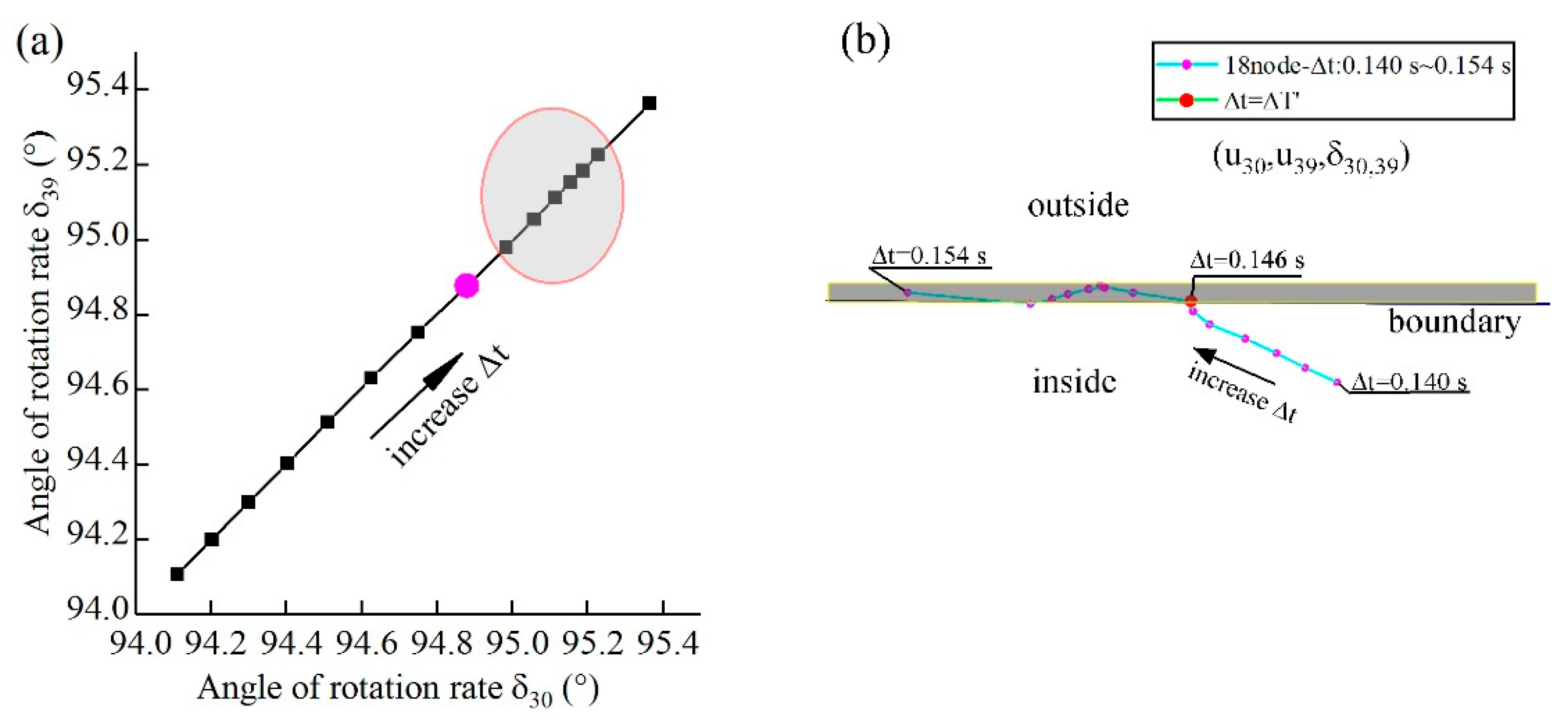
The fault clearing time $\Delta t$ increases from 0.140 s to 0.155 s. The 18-node three-phase short circuit to the ground fault. $d(\Delta t)=0.001s$.

(a). Spontaneous synchronization of meta-generators. The horizontal axis represents the fault clearing time. The vertical axis represents the standard deviation of $\delta$. The yellow area indicates the thin layer where spontaneous synchronization occurs. Here, the standard deviation $\sigma \left({\delta }_i\right)$ begins to decrease at 0.147 s (magenta) and increases by 1300% at 0.155 s (cyan) when the system is unstable. $\sigma \left({\delta }_i\right)$ can be calculated via Eq. (S6).

(b). Phenomenon of the potential barrier. $\Delta t$ increased from 0.140 s to 0.154 s. The black arrow indicates the direction in which $\Delta t$ increased. From $\Delta t=0.147s$ (the magenta dots) onward, the distance between neighboring points decreased in the direction of the black arrow (elliptical shaded area).

(c). Starting points of spontaneous synchronization. The horizontal axis represents the fault clearing time. The amplified points indicate the starting points of spontaneous synchronization. All the starting points appear at $\Delta t=0.147s$. The trends of all ${\delta }_i$ were almost identical. Combining (b) and (c) reveals that in this case, the structures in (b) exist between any two meta-generators.

We report a phenomenon of spontaneous synchronization that occurs as the system approaches the stability boundary. This is evidenced by a decrease in the standard deviation $\sigma \left({\delta }_i\right)$ (Figure 3(a)), indicating that the subsystems’ velocities spontaneously converge toward the mean value, a hallmark of synchronization [13,40]. Crucially, this self-organization is confined to a thin layer (yellow region in Figure 3(a)) immediately preceding the eventual loss of stability at $\Delta t=0.155s$. The phenomenon of spontaneous synchronization has been observed across different fault locations (Figure S4) and in distinct test systems (Figure S1), confirming its universality as an intrinsic characteristic of systems approaching the stability boundary. For power systems, this spontaneous synchronization provides a built-in and additional protection for grid stability.

The system’s trajectory in state space reveals a unique structural signature associated with this phenomenon. For a constant step size $d(\Delta t)=0.001s$, the distance between successive states decreases within the shaded area of Figure 3(b), forming a structure termed a “potential barrier” that exhibits a collective decelerating motion. This spatial manifestation of deceleration emerges precisely at the temporal onset of spontaneous synchronization, i.e., when $\sigma \left({\delta }_i\right)$ begins to decrease at $\Delta t=0.147s$ (the magenta dots correspond exactly to $\Delta t=0.147s$ in Figure 3(b).). To our knowledge, this structure has not been previously reported. A comparison between Figure S3(a) and Figure 3(b) confirms that this barrier structure is not a misleading result introduced by Equation (S2), as it is also present in the generator’s dynamic data. We hypothesize that the formation of ‘barriers’ may be related to the long-range correlations emerging near critical points within the system. This global cooperative dynamics manifests here as trajectory clustering and deceleration.

The precise timeline of spontaneous synchronization is delineated by a distinct transition in the indicator ${\displaystyle \frac{d^2{\delta }_i}{d{(\Delta t)}^2}}$. As shown in Figure 3(c), the value of ${\displaystyle \frac{d^2{\delta }_i}{d{(\Delta t)}^2}}$ for all meta-generators undergoes a simultaneous and coherent shift at $\Delta t=0.147s$ (amplified points). This timing coincides exactly with the moment when the standard deviation $\sigma \left({\delta }_i\right)$ begins to decrease in Figure 3(a), unambiguously linking the reversal in ${\displaystyle \frac{d^2{\delta }_i}{d{(\Delta t)}^2}}$ to the onset of spontaneous synchronization. Prior to this moment, ${\displaystyle \frac{d^2{\delta }_i}{d{(\Delta t)}^2}}$ remains positive; immediately afterward, ${\displaystyle \frac{d^2{\delta }_i}{d{(\Delta t)}^2}}$ becomes negative and remains so. This system-wide reversal indicates that $\Delta t=0.147s$ is the starting point of the spontaneous synchronization phase. The phase end is clearly indicated by the system’s loss of synchronization at $\Delta t=0.155s$, a state change that is demonstrated by the dramatic increase in the standard deviation $\sigma \left({\delta }_i\right)$ in Figure 3(a) and the corresponding time-domain simulation results in Figure 1(e). Thus, the metastable window of spontaneous synchronization is bounded between $\Delta t=0.147s$ and $\Delta t=0.154s$.

This newly identified spontaneous synchronization constitutes a distinct phenomenon, separate from those previously reported in power grids [11,16]. Existing phenomena typically describe how systems self-organize into synchronized states. In contrast, the novel spontaneous synchronization is uniquely characterized by its occurrence during a forward, perturbation-driven process toward instability and its association with the novel “potential barrier” structure. Second, and more critically, its emergence is strictly confined to the immediate vicinity of the synchronous stability boundary, as evidenced by experimental results under multiple fault scenarios (Figures 3(a) and S4). This refers to the situation where, during spontaneous synchronization, the position of the coordinate point $(u_K,u_L,{\delta }_{K,L})$ in the 3D coordinate system $u_K-u_L-{\delta }_{K,L}$ lies on the boundary. The intimate link between spontaneous synchronization and the stability boundary leads to a profound implication: spontaneous synchronization is independent of the underlying network. Specifically, this independence refers to the fact that its locus within the 3D coordinate system is independent of the network. We corroborate this conclusion by demonstrating the recurrence of the phenomenon in an entirely different 3-generator test system (Figure S1(a)). This independence directly undermines the traditional viewpoint in which spontaneous synchronization is fundamentally governed by network structure [41]. Moreover, the coemergence of this phenomenon with the boundary suggests that they may share a common, deep physical origin.

Our findings, particularly the diversity of behaviors near the stability boundary (e.g., contrasting outcomes in Figures 3 and S1), highlight a crucial question: how to understand the behavior of coupled oscillators before instability occurs. Key questions remain, including the specific conditions for the formation of the potential barrier and the physical determinants of the thickness of the spontaneous synchronization layer. Resolving these questions will be a primary objective of our future research.

Appendix A: Power grid datasets

This study validates the proposed method using two standard and entirely distinct power grid test systems, namely, the WECC 3-generator (3-gen) and the New England 10-generator (10-gen) systems, which differ in network topology, scale, and system parameters. The use of these fundamentally different networks is critical, as it demonstrates the broad applicability of our approach beyond any single, specific system.

For each system, the datasets comprise the dynamic parameters of the generators, the net injected real power at the generator buses, the load demand at the nongenerator buses, and the parameters of all the transmission lines and transformers. This information is sufficient for performing standard power flow and subsequent stability analyses [37].

WECC 3-generator test system (3-gen) [29]. This system represents the Western System Coordinating Council (WSCC), which is part of the region now named the Western Electricity Coordinating Council (WECC) in the North American power grid. There are 3 generators in the system.

New England test system (10-gen) [30]. The IEEE 39-bus system is the 10-machine New England Power System. The prototype of the IEEE 39-node system is a model of an actual power grid in New England. There are 10 generators in the system.

The simulation results from these datasets are presented throughout the paper, with the New England system results primarily shown in Figures 1, 3, and S2-S5, and Table S1, and the 3-generator system results in Figures 2 and S1.

Appendix B: Derivation of the boundary equation

The boundary equation with ${\omega }_0$

Synchronization emerges when the suppression (of the loss of synchrony) dominates dissimilarity. This is a simple principle (or consensus) regarding synchronization [2]. Here, suppression includes the effects of coupling and dissipation.

The suppression strength between the nodes is quantified by $P_{\Delta u}$, and the dissimilarity between the nodes is quantified by $P_{\partial u}$. $P_{\Delta u}$ and $P_{\partial u}$ have the same dimension and can be directly compared in size. As a natural corollary of the consensus, the boundary is defined by the equality between the suppression and the dissimilarity. Thus, the synchronization stability boundary equation is expressed as $P_{\Delta u}=P_{\partial u}$. When $\left|P_{\partial u}\right|\le \left|P_{\Delta u}\right|$, the system is synchronous and stable. Conversely, when $\left|P_{\partial u}\right|>\left|P_{\Delta u}\right|$, the system is out of synchronization and unstable.

Figure 1. Schematic representation of the key quantities $\Delta u$ and $\partial u$ in the polar coordinate system.

Figure 1. Schematic representation of the key quantities $\Delta u$ and $\partial u$ in the polar coordinate system.

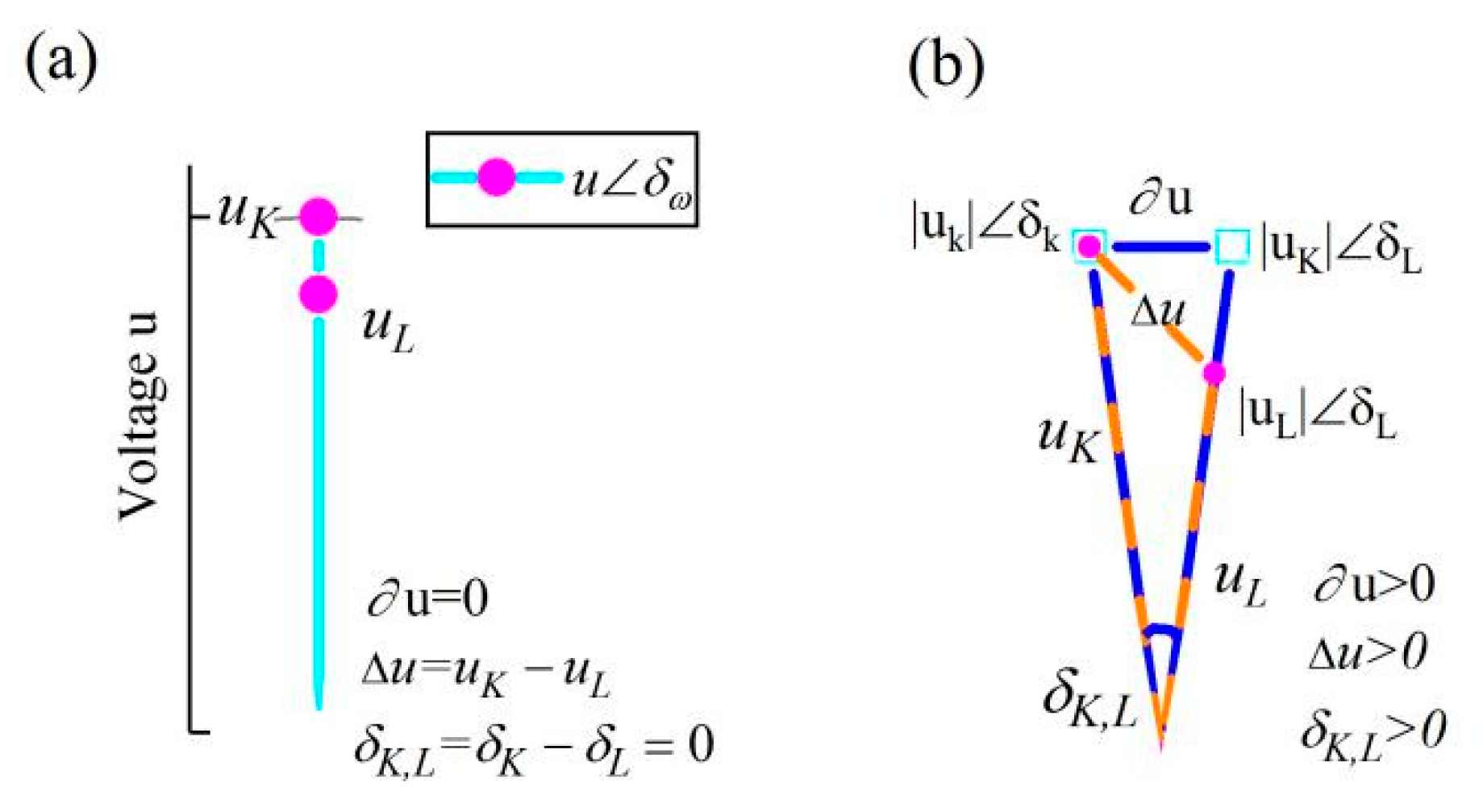
Fig. B1 provides an analogical interpretation using a phasor diagram for power system analysis. $\Delta u$ represents the “suppression potential difference”, while $\partial u$ represents the “dissimilar potential difference” between the K-th and L-th generators. $\left|\Delta u\right|$ and $\left|\partial u\right|$ are calculated via Eq. (B3).

(a). Steady state during synchronous operation. Each magenta dot represents the coordinate of the i-th meta-generator $\left|u_i\right|\angle {\delta }_i$. The cyan line has a length equal to the generator’s voltage $u_i$. The angle of rotation rate (ARR) ${\delta }_i$ of this line is defined by the generator’s rotation rate, which is calculated as ${\delta }_i=2\arctan ({\omega }_i^{*})=2\arctan ({\displaystyle \frac{{\omega }_i}{{\omega }_0}})$. Here, ${\omega }_i^{*}$ is the normalized rotation rate, where ${\omega }_i$ is the actual value and ${\omega }_0$ is the power system base frequency. When all the generators are synchronized, the case is characterized by ${\delta }_{K,L}=0,\left|\Delta u\right|\ge \left|\partial u\right|=0$.

(b). State during asynchronous operation. The length of the orange dotted line between the magenta square dots represents the magnitude of $\Delta u$, and the length of the solid blue line between the cyan dots represents the magnitude of $\partial u$. When the generator frequencies differ, the case is characterized by ${\delta }_{K,L}>0,\left|\Delta u\right|>0,\left|\partial u\right|>0$.

The algebraic and geometric models of the voltage phasor diagram, which plays a critical role in power system analysis, provided inspiration for the expressions of $P_{\Delta u}$ and $P_{\partial u}$. The expressions for $P_{\Delta u}$ and $P_{\partial u}$ are analogous to those of $P_{K,L}={\displaystyle \frac{{\left|{\stackrel{\rightharpoonup }{U}}_K-{\stackrel{\rightharpoonup }{U}}_L\right|}^2}{\left|Z_{K,L}\right|}}$, which represents the rate of energy dissipation between the nodes in a power system.

$$P_{\Delta u}={\displaystyle \frac{{\left|{\overrightarrow{u}}_K-{\overrightarrow{u}}_L\right|}^2}{\left|Z_{K,L}\right|}}={\displaystyle \frac{{\left|\Delta u\right|}^2}{\left|Z_{K,L}\right|}}$$

(B1)

and

$$P_{\partial u}={\displaystyle \frac{{\left|{\overrightarrow{u}}_K-\frac{\left|{\overrightarrow{u}}_K\right|}{\left|{\overrightarrow{u}}_L\right|}{\overrightarrow{u}}_L\right|}^2}{\left|Z_{K,L}\right|}}={\displaystyle \frac{{\left|\partial u\right|}^2}{\left|Z_{K,L}\right|}}$$

(B2)

[see Fig. B1(b)]. $Z_{K,L}$ represents the impedance between the Kth and the Lth generators. The difference between ${\stackrel{\rightharpoonup }{u}}_i$ and $\stackrel{\rightharpoonup }{U}$ in a physical sense is that the ARR ${\delta }_i$ of ${\stackrel{\rightharpoonup }{u}}_i$ is defined by the frequency ${\omega }_i$, whereas the angle ${\theta }_i$ of $\stackrel{\rightharpoonup }{U}$ represents the phase angle.

The expressions of $P_{\Delta u}$ and $P_{\partial u}$ indicate that they are related to the network because information about the network is contained in $Z_{K,L}$ (e.g., the adjacency matrix and system parameters). However, for any two generators K and L, $Z_{K,L}$ is the same in the expressions of $P_{\Delta u}$ and $P_{\partial u}$. $\left|P_{\partial u}\right|/\left|P_{\Delta u}\right|=1$ eliminates $Z_{K,L}$. Therefore, the boundary equation $\left|P_{\partial u}\right|/\left|P_{\Delta u}\right|=1$ is independent of disturbances, network topology, and system parameters. Although these factors collectively determine the system’s dynamic trajectory and generator operating points, the mathematical form and geometrical shape of the stability boundary itself remain invariant. Combining Eqs. (B1) and (B2), it is observed that $\left|P_{\partial u}\right|/\left|P_{\Delta u}\right|=1\iff \left|\partial u\right|/\left|\Delta u\right|=1$. The set of points for which $\left|\partial u\right|=\left|\Delta u\right|$ is the synchronous stability boundary.

As shown in Fig. B1(b),

$$\begin{array}{l}\left|\Delta u\right|=\left|{\overrightarrow{u}}_K-{\overrightarrow{u}}_L\right|=\sqrt{{\left|{\overrightarrow{u}}_K\right|}^2+{\left|{\overrightarrow{u}}_L\right|}^2-2\left|{\overrightarrow{u}}_K\right|\left|{\overrightarrow{u}}_L\right|\cos {\delta }_{K,L}},\\ \left|\partial u\right|=\left|{\overrightarrow{u}}_K-{\displaystyle \frac{\left|{\overrightarrow{u}}_K\right|}{\left|{\overrightarrow{u}}_L\right|}}{\overrightarrow{u}}_L\right|=\sqrt{2{\left|{\overrightarrow{u}}_K\right|}^2(1-\cos {\delta }_{K,L})}.\end{array}$$

(B3)

The symbols “∆” and “$\partial$“ are for distinction only and have no mathematical significance. Thus, the boundary equation is obtained via derivation from ${\left|{\overrightarrow{u}}_K\right|}^2+{\left|{\overrightarrow{u}}_L\right|}^2-2\left|{\overrightarrow{u}}_K\right|\left|{\overrightarrow{u}}_L\right|\cos {\delta }_{K,L}=2{\left|{\overrightarrow{u}}_K\right|}^2(1-\cos {\delta }_{K,L})$. The only variables in the boundary equation are $u_K,u_L$ and ${\delta }_{K,L}$. These physical quantities are all representations of individual behavior.

$f\left(u_K,u_L,{\delta }_{K,L}\right)=\left|\partial u\right|/\left|\Delta u\right|=1$ is the stability boundary equation. When $\left|\partial u\right|/\left|\Delta u\right|<1$, the system is stable. When $\left|\partial u\right|/\left|\Delta u\right|>1$, the system is unstable. Geometrically, $f\left(u_K,u_L,{\delta }_{K,L}\right)=1$ describes exactly curved surfaces that, together with $(0,u_L,{\delta }_{K,L})$, $(u_K,0,{\delta }_{K,L})$ and $(u_K,u_L,0)$ enclose a stable domain.

The boundary equation

$$\left|u_K\right|=\left|u_L\right|\cup {\displaystyle \frac{\left|u_L\right|}{\left|u_K\right|}}=2\cos {\delta }_{K,L}-1$$

where $\left|u_K\right|\ge \left|u_L\right|\ge 0,\left|{\delta }_{K,L}\right|\ge 0$. This is Eq. (1) in the main text.

The coordinate system $u_K-u_L-{\delta }_{K,L}$ is established, and the boundary is visualized (Figure 1(a)).

It should be noted that this boundary equation originated from physical intuition and the analysis of simulation data. We observed from the data that the quantity defined by Eq. (B3), where $\left|\partial u\right|=\left|\Delta u\right|$, precisely determines power system stability. This regularity suggested that it could be incorporated into the established physical consensus that “synchronization is determined by a balance between the suppression and the dissimilarity.” Based on this insight, we developed a theoretical framework for $P_{\Delta u}$ and $P_{\partial u}$. The construction of this framework yields an immediate theoretical consequence: the parameter $Z_{K,L}$, which contains network information, is naturally eliminated under the condition $\left|P_{\partial u}\right|/\left|P_{\Delta u}\right|=1$, which is equivalent to $\left|\partial u\right|/\left|\Delta u\right|=1$. Consequently, the framework presented in this paper not only unifies empirical observations with physical principles but also reveals the profound property that the stability boundary is independent of the network.

Appendix C: The boundary equation without ${\omega }_0$

As mentioned in the derivation above, ${\delta }_i=2\arctan ({\omega }_i^{*})=2\arctan ({\displaystyle \frac{{\omega }_i}{{\omega }_0}})$, where ${\omega }_0$ represents the power system base frequency and ${\omega }_i$ denotes the actual value. ${\omega }_0$ is constrained to positive real numbers. For a power system, the base frequency generally coincides with the rated frequency of the system(50 Hz or 60 Hz in most power grids globally). As previously stated in this paper, ${\omega }_0=50Hz$. ${\omega }_0$ is used extensively in power system analysis. However, to some extent, the selection of ${\omega }_0$ remains “anthropic selective”. Additionally, ${\omega }_0$ may be unknown before synchronization emerges. Can ${\omega }_0$ be eliminated from the boundary equation (i.e., is there a synchronization stability boundary independent of ${\omega }_i$ for power systems)?

When ${\delta }_i=2\arctan {\displaystyle \frac{{\omega }_i}{{\omega }_0}}$ is substituted into Eq. (1),

$${\displaystyle \frac{1}{2}}({\displaystyle \frac{\left|u_L\right|}{\left|u_K\right|}}+1)=\cos [2(\arctan {\displaystyle \frac{{\omega }_K}{{\omega }_0}}-\arctan {\displaystyle \frac{{\omega }_L}{{\omega }_0}})]$$

(C1)

Considering $\cos 2\alpha ={\displaystyle \frac{1-{\tan }^2\alpha }{1+{\tan }^2\alpha }}$ and $\tan (\alpha -\beta )={\displaystyle \frac{\tan \alpha -\tan \beta }{1+\tan \alpha \tan \beta }}$,

$${\displaystyle \frac{1}{2}}({\displaystyle \frac{\left|u_L\right|}{\left|u_K\right|}}+1)={\displaystyle \frac{{\left({{\omega }_0}^2+{\omega }_K{\omega }_L\right)}^2-{{\omega }_0}^2{\left({\omega }_K-{\omega }_L\right)}^2}{{\left({{\omega }_0}^2+{\omega }_K{\omega }_L\right)}^2+{{\omega }_0}^2{\left({\omega }_K-{\omega }_L\right)}^2}}$$

(C2)

By setting $A^{\prime }=\sqrt{{\displaystyle \frac{\left|u_K\right|-\left|u_L\right|}{3\left|u_K\right|+\left|u_L\right|}}},B^{\prime }={\omega }_L-{\omega }_K,C^{\prime }={\omega }_L{\omega }_K\sqrt{{\displaystyle \frac{\left|u_K\right|-\left|u_L\right|}{3\left|u_K\right|+\left|u_L\right|}}}$, Eq. (C2) becomes $A^{\prime }{{\omega }_0}^2+B^{\prime }{\omega }_0+C^{\prime }=0$. Therefore,

$${{\omega }_0}_{1,2}={\displaystyle \frac{{\omega }_K-{\omega }_L\pm \sqrt{{\left({\omega }_K-{\omega }_L\right)}^2-4\frac{\left|u_K\right|-\left|u_L\right|}{3\left|u_K\right|+\left|u_L\right|}{\omega }_L{\omega }_K}}{2\sqrt{\frac{\left|u_K\right|-\left|u_L\right|}{3\left|u_K\right|+\left|u_L\right|}}}}$$

(C3)

For real-world systems, both ${\omega }_{01}$ and ${\omega }_{02}$ must be real numbers. This fact provides the basis for proving the boundary equation (see appendix D). There is a constraint that ${\left({\omega }_K-{\omega }_L\right)}^2-4{\displaystyle \frac{\left|u_K\right|-\left|u_L\right|}{3\left|u_K\right|+\left|u_L\right|}}{\omega }_L{\omega }_K\ge 0$. Therefore, the power system is synchronously stable when

$$0\le 1-{\displaystyle \frac{4{\left({\omega }_K-{\omega }_L\right)}^2}{{\left({\omega }_K+{\omega }_L\right)}^2}}\le {\displaystyle \frac{\left|u_L\right|}{\left|u_K\right|}}\le 1.$$

(C4)

In Eq. (C4), Condition $0\le 1-{\displaystyle \frac{4{\left({\omega }_K-{\omega }_L\right)}^2}{{\left({\omega }_K+{\omega }_L\right)}^2}}$, which is derived from Constraint $A^{\prime }{{\omega }_0}^2+B^{\prime }{\omega }_0+C^{\prime }\ge 0$ and is ultimately driven by the requirement of ${\displaystyle \frac{\left|u_L\right|}{\left|u_K\right|}}\le 2\cos {\delta }_{K,L}-1$.

$$1-{\displaystyle \frac{4{\left({\omega }_K-{\omega }_L\right)}^2}{{\left({\omega }_K+{\omega }_L\right)}^2}}={\displaystyle \frac{\left|u_L\right|}{\left|u_K\right|}}$$

(C5)

is the stability boundary without ${\omega }_0$. When $u_K=u_L$, any value chosen for ${\omega }_K-{\omega }_L\ge 0$ satisfies Eq. (C4). $u_K=u_L$ is exactly the left side of Eq. (1). When $u_K\ne u_L$, Eq. (C5) is equivalent to the right side of Eq. (1). Eq. (1) and Eq. (C5) are equivalent [see appendix E]. This boundary equation is still determined by the behavior of individuals in the system and is independent of the network.

A comparison of Eq. (1) indicates that Eq. (C5) has a larger range of applicability because Eq. (1) requires prior knowledge of the value of ${\omega }_0$. However, for convenience, this paper still uses Eq. (1) for visualization, as shown in Figure 1(a).

This boundary equation originates from physical intuition and analogy. Its rigor was subsequently established through experimental validation and mathematical proofs. The experimental validation results are provided in Figures 1, 2, S2, S3(b) and S5, among others.

Appendix D: Proof of the boundary equation

We prove that Eqs. (1) and (C5) describe the stability boundary. The proof proceeds as follows:

The proof proceeds in two steps. First, we prove that Eq. (C5) represents the boundary. We then prove that Eq. (1) is equivalent to Eq. (C5). Therefore, Eq. (1) is also shown to represent the boundary.

Definitions:

A Domain: Variables are ${\omega }_K,{\omega }_L\in R$, with ${\omega }_K>{\omega }_L>0$. ${\omega }_K,{\omega }_L$ represents the frequency of the generator.

B Domain: Variables are ${\omega }_{01},{\omega }_{02}$. ${\omega }_{01},{\omega }_{02}$ are the two roots of a quadratic equation $A^{\prime }{{\omega }_0}^2+B^{\prime }{\omega }_0+C^{\prime }=0$. ${\omega }_0$ represents the common frequency of the power system. The quadratic equation originates from an independent consensus: Synchronization emerges when the suppression dominates dissimilarity.

There exists a pair of invertible algebraic maps, $F$ (see Eq. C3) and $F^{-1}$, that establish complete equivalence between the two domains: Let $A=2\sqrt{{\displaystyle \frac{\left|u_K\right|-\left|u_L\right|}{3\left|u_K\right|+\left|u_L\right|}}}$.

Forward Map $F:({\omega }_K,{\omega }_L)\mapsto ({\omega }_{01},{\omega }_{02})$,

$$\begin{array}{l}{{\omega }_0}_1=F_1({\omega }_K,{\omega }_L,A)={\displaystyle \frac{{\omega }_K-{\omega }_L+\sqrt{{\left({\omega }_K-{\omega }_L\right)}^2-4A^2{\omega }_L{\omega }_K}}{2A}},\\ {{\omega }_0}_2=F_2({\omega }_K,{\omega }_L,A)={\displaystyle \frac{{\omega }_K-{\omega }_L-\sqrt{{\left({\omega }_K-{\omega }_L\right)}^2-4A^2{\omega }_L{\omega }_K}}{2A}}.\end{array}$$

Inverse Map $F^{-1}:({\omega }_{01},{\omega }_{02})\mapsto ({\omega }_K,{\omega }_L)$,

$$\begin{array}{l}{\omega }_K=f_3({\omega }_{01},{\omega }_{02},A)={\displaystyle \frac{\sqrt{A^2{\left({\omega }_{01}+{\omega }_{02}\right)}^2+4{\omega }_{01}{\omega }_{02}}+A({\omega }_{01}+{\omega }_{02})}{2}},\\ {\omega }_L=f_4({\omega }_{01},{\omega }_{02},A)={\displaystyle \frac{\sqrt{A^2{\left({\omega }_{01}+{\omega }_{02}\right)}^2+4{\omega }_{01}{\omega }_{02}}-A({\omega }_{01}+{\omega }_{02})}{2}}.\end{array}$$

The Principle of Real Numbers: The value of the common frequency ${\omega }_0$ must be a real number. This stems from an uncontested consensus: For each generator, the measured frequency value must be a real number. Since the common frequency emerges from these individual frequencies, it must consequently be real.

Proof:

The maps $F$ and $F^{-1}$ establish one-to-one correspondence between the A domain and the B domain within their domains of definition. Thus, the two systems are algebraically equivalent. The analysis of the A domain can be transformed entirely equivalently into the analysis of the B domain.

Define the discriminant:$\Delta ={\left({\omega }_K-{\omega }_L\right)}^2-4A^2{\omega }_L{\omega }_K$.

From the expressions of map $F$, ${\omega }_{01}\in R$ and ${\omega }_{02}\in R$ are real if and only if ${\left({\omega }_K-{\omega }_L\right)}^2-4A^2{\omega }_L{\omega }_K\ge 0$, i.e., $\Delta \ge 0$. If $\Delta <0$, ${\omega }_{01},{\omega }_{02}$ are complex numbers.

In according with the principle of real numbers, the common frequency ${\omega }_0$ must be a real number. ${\omega }_{01},{\omega }_{02}$ are two solutions to ${\omega }_0$. This strictly requires that both ${\omega }_{01}\in R$ and ${\omega }_{02}\in R$ must be true. This requirement defines a boundary for the physically admissible region in domain B. The boundary is described by $\Delta =0$. Therefore, all physically realizable states must and can only lie within the region satisfying $\Delta \ge 0$ (Physically Admissible Domain).

On the basis of the principle of real numbers and the equivalence of the A and B domains, we can rigorously define the existence limit of synchronization:

Admissible domain: Regions in the A domain that are equivalent to those in the B domain where $\Delta >0$.

Boundary: Regions in the A domain that are equivalent to those in the B domain where $\Delta =0$.

Forbidden domain: Regions in the A domain that are equivalent to those in the B domain where $\Delta <0$. The system state cannot remain stable.

Thus, the equation is as follows:

$${\left({\omega }_K-{\omega }_L\right)}^2-4A^2{\omega }_L{\omega }_K=0$$

strictly delineates the physically achievable region from the physically unachievable region. It constitutes the admissible boundary of the system. This is precisely Eq. (C5), which is equivalent to Eq. (1) (when ${\omega }_K\approx {\omega }_L$ is true). Therefore, Eq. (1) is also proven to be the stability boundary.

Explanation:

In fact, the equivalence between the synchronously admissible boundary and the mathematical description of the principle of real numbers is shown here. Eq. (C5) is precisely the mathematical expression of that principle. The boundary of the physically admissible domain defines the existence of system states and thus carries more profound implications. Logically, physical admissibility is the cornerstone for discussing stability: A state must physically exist before its stability can be discussed. Our work not only established this boundary but also revealed its remarkable independence from the network.

In this paper, the physically admissible region is interpreted as the stability region. Although the admissible boundary and the stability boundary are not conceptually identical, their equivalence in the context of power systems does not compromise the rigor of this paper for the following reasons:

1, Stability refers to a system’s ability to return to an equilibrium state after being subjected to a disturbance. As detailed in the “experimental steps” section, a disturbance (fault) is applied to a synchronized power system at an engineering-acceptable step size ($d(\Delta t)=0.001$ s) until the generator system loses synchronization. This demonstrates that the experimental design aligns with the concept of stability. This experimental design also indicates that even if the two boundaries do not perfectly coincide, their discrepancy falls within the acceptable resolution for power systems.

2, All the experimental results demonstrate the successful application of the boundary to synchronization issues, including stability assessment and the multiswing stability for multiple generators. In experiments with different network topologies and disturbance scenarios, the observed stability discrimination results precisely matches the simulation experiments (refer to Figures 1, 2 and S5).

This study reveals that the synchronization stability boundaries are constrained by the principle of real numbers. Here, the direct contribution of this mathematical proof lies in enabling us to understand a counterintuitive conclusion: the synchronous stability boundary is independent of any particular network. More profoundly, the boundary equation is directly grounded in fundamental principles of physics, thereby transcending specific network structures.

Appendix E: Proof of Equivalence Between Eqs. (1) and (C5)

Proof:

Eq. (1) transforms equivalently to Eq. (C2): The derivation from Eq. (1) to Eq. (C2) is presented in “The boundary equation without ${\omega }_0$”. According to this derivation process, when $\left|u_K\right|\ge \left|u_L\right|,{\omega }_K-{\omega }_L\ge 0$, Eq. (1) is clearly equivalent to Eq. (C2).

Eq. (C5) transforms equivalently to Eq. (C2): Eq. (C5) becomes ${\displaystyle \frac{1}{2}}({\displaystyle \frac{\left|u_L\right|}{\left|u_K\right|}}+1)=1-{\displaystyle \frac{2{\left({\omega }_K-{\omega }_L\right)}^2}{{\left({\omega }_K+{\omega }_L\right)}^2}}$. Expanding the right-hand side of the above equation yields ${\displaystyle \frac{-{\omega }_K^2+6{\omega }_K{\omega }_L-{\omega }_L^2}{{({\omega }_K+{\omega }_L)}^2}}$, which is expressed as $={\displaystyle \frac{4{\omega }_K{\omega }_L-{\left({\omega }_K-{\omega }_L\right)}^2}{4{\omega }_K{\omega }_L+{\left({\omega }_K-{\omega }_L\right)}^2}}={\displaystyle \frac{{\omega }_K{\omega }_L[4{\omega }_K{\omega }_L-{\left({\omega }_K-{\omega }_L\right)}^2]}{{\omega }_K{\omega }_L[4{\omega }_K{\omega }_L+{\left({\omega }_K-{\omega }_L\right)}^2]}}$. Let $X=\sqrt{{\omega }_K{\omega }_L}$, then ${\displaystyle \frac{4X^4-X^2{\left({\omega }_K-{\omega }_L\right)}^2}{4X^4+X^2{\left({\omega }_K-{\omega }_L\right)}^2}}={\displaystyle \frac{{\left(X^2+{\omega }_K{\omega }_L\right)}^2-X^2{\left({\omega }_K-{\omega }_L\right)}^2}{{\left(X^2+{\omega }_K{\omega }_L\right)}^2+X^2{\left({\omega }_K-{\omega }_L\right)}^2}}$. When ${\omega }_K\approx {\omega }_L$, that is ${\omega }_K-{\omega }_L<<{\omega }_L\le {\omega }_K$, denote $X$ by ${\omega }_0$ [when the system is stable, ${\omega }_K-{\omega }_L<<{\omega }_L\le {\omega }_K$ is true (see Table K1 and other data in “Data availability”)]. The right-hand side of the above equation coincides with the right-hand side of Eq. (C2), hence ${\displaystyle \frac{1}{2}}({\displaystyle \frac{\left|u_L\right|}{\left|u_K\right|}}+1)={\displaystyle \frac{{\left({{\omega }_0}^2+{\omega }_K{\omega }_L\right)}^2-{{\omega }_0}^2{\left({\omega }_K-{\omega }_L\right)}^2}{{\left({{\omega }_0}^2+{\omega }_K{\omega }_L\right)}^2+{{\omega }_0}^2{\left({\omega }_K-{\omega }_L\right)}^2}}$. Eq. (C5) is equivalent to Eq. (C2).

Both Eqs. (1) and (C5) are both equivalent to Eq. (C2). Therefore, when $\left|u_K\right|\ge \left|u_L\right|,{\omega }_K-{\omega }_L\ge 0$, and ${\omega }_K-{\omega }_L<<{\omega }_L\le {\omega }_K$, Eq. (1) and Eq. (C5) are equivalent.

Appendix F: Proof that Eq. (S2) does not alter the stability criterion of the system

The section on “Stability Boundary” employs meta-generators to validate the boundary equation. This raises a critical question: could the transformation from a generator to a meta-generator introduce erroneous results that invalidate the verification? In other words, regarding the criterion for synchronous stability, are the two models equivalent before and after the application of Eq. (S2)?

Definitions:

Definition 1: All analyses are conducted within any fixed time window $\left[T^{\prime },T^{\prime }+T\right]$. During this time window, define $\alpha T$ as the total duration of periods where ${{\delta }^{\prime }}_i(t)>{{\delta }^{\prime }}_j(t)$, and conversely, define $(1-\alpha )T$ as the total duration of periods where ${{\delta }^{\prime }}_i(t)<{{\delta }^{\prime }}_j(t)$. Then, $\alpha \in \left[0,1\right]$ and $T=\alpha T+(1-\alpha )T$. ${{\delta }^{\prime }}_i(t)$ represents the instantaneous values of the ARR of ith generator.

Definition 2 (the stability of the generator system): The difference in the ARR of generator is defined as ${{\delta }^{\prime }}_i-{{\delta }^{\prime }}_j={\displaystyle \frac{1}{T}}{\displaystyle {\int }_I[{{\delta }^{\prime }}_i(t)-{{\delta }^{\prime }}_j}(t)]dt$. For $\forall \epsilon >0$, the stability criterion is $\epsilon >0$ and the system is stable if and only if $‖{{\delta }^{\prime }}_i-{{\delta }^{\prime }}_j‖\le \epsilon$.

Definition 3 (the stability of the meta-generator system): According to Eq. (S2) and Definition 1, the ARRs of the meta-generator are defined as ${\delta }_i={\displaystyle \frac{1}{T}}{\displaystyle {\int }_I[\alpha {{\delta }^{\prime }}_i(t)+(1-\alpha ){{\delta }^{\prime }}_j}(t)]dt$ (the ith meta-generator) and ${\delta }_j={\displaystyle \frac{1}{T}}{\displaystyle {\int }_I[(1-\alpha ){{\delta }^{\prime }}_i(t)+\alpha {{\delta }^{\prime }}_j}(t)]dt$ (the jth meta-generator). Their difference is $‖{\delta }_i-{\delta }_j‖$. The stability criterion uses the same $\epsilon$ as definition 2 does. The system is stable if and only if $‖{\delta }_i-{\delta }_j‖\le \epsilon$.

Proof:

From the definitions above, it is directly derived that: $‖{\delta }_i-{\delta }_j‖=\left(2\alpha -1\right)‖{{\delta }^{\prime }}_i-{{\delta }^{\prime }}_j‖$. According to Eq. (S2), ${\delta }_i-{\delta }_j\ge 0$. We assume that within the time window, ${{\delta }^{\prime }}_i(t)>{{\delta }^{\prime }}_j(t)$ holds most of the time, implying that $\alpha \in \left[{\displaystyle \frac{1}{2}},1\right]$. For any two generators, ${{\delta }^{\prime }}_i(t)$ and ${{\delta }^{\prime }}_j(t)$ can always be selected. Therefore, this assumption does not lose generality and is always reasonable.

Theorem (stability assessment equivalence): Under the framework of Definitions 1–3, the generator system is synchronously stable if and only if the meta-generator system is synchronously stable.

The proof is completed by demonstrating the following two corollaries.

Corollary 1 (preservation of stability): If the generator system is stable ($‖{{\delta }^{\prime }}_i-{{\delta }^{\prime }}_j‖\le \epsilon$), then the meta-generator system is stable ($‖{\delta }_i-{\delta }_j‖\le \epsilon$).

Proof: From $‖{\delta }_i-{\delta }_j‖=\left(2\alpha -1\right)‖{{\delta }^{\prime }}_i-{{\delta }^{\prime }}_j‖$ and the fact that $\alpha \in \left[{\displaystyle \frac{1}{2}},1\right]$ implies $2\alpha -1\le 1$, it follows that $‖{\delta }_i-{\delta }_j‖=\left(2\alpha -1\right)‖{{\delta }^{\prime }}_i-{{\delta }^{\prime }}_j‖\le \epsilon$. Therefore, the meta-generator system is stable.

Corollary 2 (preservation of instability): If the generator system is unstable ($‖{{\delta }^{\prime }}_i-{{\delta }^{\prime }}_j‖>\epsilon$), then the meta-generator system is unstable ($‖{\delta }_i-{\delta }_j‖>\epsilon$).

Proof: The instability of the generator system ($‖{{\delta }^{\prime }}_i-{{\delta }^{\prime }}_j‖>\epsilon$) physically corresponds to a significant difference in the frequencies of the two generators, i.e., a loss of synchronization. This loss of synchronization implies that the state of one generator is persistently greater than that of the other for the vast majority of the observation window, indicating that the parameter $\alpha \to 1$. Substituting $\alpha =1$ into the core identity $‖{\delta }_i-{\delta }_j‖=\left(2\alpha -1\right)‖{{\delta }^{\prime }}_i-{{\delta }^{\prime }}_j‖$ yields $‖{\delta }_i-{\delta }_j‖=‖{{\delta }^{\prime }}_i-{{\delta }^{\prime }}_j‖$ [refer to Figures 1(f), 2(e), S5(c), (f) and (l)]. Therefore, $‖{\delta }_i-{\delta }_j‖=‖{{\delta }^{\prime }}_i-{{\delta }^{\prime }}_j‖>\epsilon$, and the meta-generator system is unstable.

The two systems are equivalent in stability assessment; that is, Eq. (S2) does not change the stability discrimination of the system. The proof applies to a two-generator system.

Definitions:

Depending on the fault and network conditions, a multigenerator system may form completely different synchronous clusters upon instability, which greatly complicates the analysis of its synchronous stability.

We now prove that the generator system and the meta-generator system retain the same stability even when extended to multiple generators.

Definition 4 (the $\alpha$ matrix): In the case of multiple generators, $\alpha$ in Definition 1 is replaced by the $\alpha$ matrix $\alpha ={({\alpha }_{ij})}_{n\times n}$. There is

$$\left[\begin{array}{c}{\delta }_1\\ {\delta }_2\\ ⋮\\ {\delta }_n\end{array}\right]=\left[\begin{array}{cccc}{\alpha }_{11}& {\alpha }_{12}& \dots & {\alpha }_{1n}\\ {\alpha }_{21}& {\alpha }_{22}& \dots & {\alpha }_{2n}\\ ⋮& ⋮& \ddots & ⋮\\ {\alpha }_{n1}& {\alpha }_{n2}& \dots & {\alpha }_{nn}\end{array}\right]\left[\begin{array}{c}{{\delta }^{\prime }}_1\\ {{\delta }^{\prime }}_2\\ ⋮\\ {{\delta }^{\prime }}_n\end{array}\right]$$

The matrix $\alpha ={({\alpha }_{ij})}_{n\times n}$ satisfies all ${\alpha }_{ij}\ge 0$. For any i: ${\alpha }_{i1}+{\alpha }_{i2}+\dots +{\alpha }_{in}=1$ and ${\alpha }_{1i}+{\alpha }_{2i}+\dots +{\alpha }_{ni}=1$.

Definition 5 (the stability of the multigenerator system): The power system comprises n generators, which form the set $G^{\prime }=\{{G^{\prime }}_1,{G^{\prime }}_2,\dots {G^{\prime }}_n\}$. For $\forall \epsilon >0$, the stability criterion is $\epsilon >0$. The system is synchronously stable if and only if for any subset $\{{G^{\prime }}_i,{G^{\prime }}_j\}$, $‖{{\delta }^{\prime }}_i-{{\delta }^{\prime }}_j‖\le \epsilon$ holds. For a power system with n generators, there are $n(n-1)$ subsets.

Definition 6 (the stability of the n meta-generator system): By definition, there are also n meta-generators. These meta-generators form an ordered set, $MG=\{M{G}_1,\dots ,M{G}_K,M{G}_L,\dots M{G}_n\}$. Adjacent meta-generators are defined as ordered subsets $\{M{G}_K,M{G}_L\}$ within this set. L=K+1. The stability criterion uses the same $\epsilon$ as definition 5 does. The meta-generator system is stable if and only if all adjacent meta-generators $\{M{G}_K,M{G}_L\}$ are stable, i.e., $‖{\delta }_K-{\delta }_L‖\le \epsilon$. There are (n-1) ordered sets of $\{M{G}_K,M{G}_L\}$.

Proof:

Theorem (stability assessment equivalence): The multigenerator system is synchronously stable if and only if the n meta-generator system is synchronously stable.

The proof is completed by demonstrating the following two corollaries.

Corollary 1 (preservation of stability): If the multigenerator system is stable, then the n meta-generator system is stable.

Proof: For any two generators $\{{G^{\prime }}_i,{G^{\prime }}_j\}$, $‖{{\delta }^{\prime }}_i-{{\delta }^{\prime }}_j‖\le \epsilon$ holds when the system is stable. That is, $\max {\delta }^{\prime }-\min {\delta }^{\prime }\le \epsilon$. Let $M=\max {\delta }^{\prime },m=\min {\delta }^{\prime }$; then, $M-m\le \epsilon$.

For the ith and i+1th meta-generators, ${\delta }_i={\displaystyle \sum _{k=1}^n{\alpha }_{ik}}{{\delta }^{\prime }}_k$ and ${\delta }_{i+1}={\displaystyle \sum _{k=1}^n{\alpha }_{(i+1)k}}{{\delta }^{\prime }}_k$. Therefore, ${\delta }_i-{\delta }_{i+1}={\displaystyle \sum _{k=1}^n[{\alpha }_{ik}-{\alpha }_{(i+1)k}]}{{\delta }^{\prime }}_k$. Let $d_k={\alpha }_{ik}-{\alpha }_{(i+1)k}$; then, ${\displaystyle \sum _{k=1}^n{d}_k}=1-1=0$. Let ${{\delta }^{\prime }}_k=m+t_k(M-m)$, where $0\le t_k\le 1$ and $M-m\le \epsilon$. Substitute: ${\delta }_i-{\delta }_{i+1}={\displaystyle \sum _k{d}_k[m+t_k(M-m)]}=(M-m){\displaystyle \sum _k{d}_k{t}_k}$.

Let $S^{+}=\{k:d_k>0\}$, $S^{-}=\{k:d_k<0\}$. From ${\displaystyle \sum _{k=1}^n{d}_k}=0$, we obtain ${\displaystyle \sum _{k\in S^{+}}{d}_k}=-{\displaystyle \sum _{k\in S^{-}}{d}_k}=\Phi$, where $\Phi ={\displaystyle \frac{1}{2}}{\displaystyle \sum _{k=1}^n\left|d_k\right|}$. Then ${\displaystyle \sum _k{d}_k{t}_k}\le {\displaystyle \sum _{k\in S^{+}}{d}_k}*1+{\displaystyle \sum _{k\in S^{-}}{d}_k*0}=\Phi$ and ${\displaystyle \sum _k{d}_k{t}_k}\ge {\displaystyle \sum _{k\in S^{+}}{d}_k}*0+{\displaystyle \sum _{k\in S^{-}}{d}_k*1}=-\Phi$. so that $\left|{\displaystyle \sum _k{d}_k{t}_k}\right|\le \Phi$.

For the vectors ${\alpha }_{i•}$ and ${\alpha }_{(i+1)•}$, ${\displaystyle \sum _{k=1}^n\left|{\alpha }_{ik}-{\alpha }_{(i+1)k}\right|}\le 2$. Thus $\Phi ={\displaystyle \frac{1}{2}}{\displaystyle \sum _{k=1}^n\left|d_k\right|}\le 1$. Therefore $‖{\delta }_i-{\delta }_{i+1}‖\le (M-m)*\Phi \le \epsilon *1=\epsilon$. According to the Definition 6, the meta-generator system is stable.

Corollary 2 (preservation of instability): If the multigenerator system is unstable, then the meta-generator system is unstable.

Proof: According to definition 5, the multigenerator system instability indicates that at least one generator ${G^{\prime }}_k$ has lost stability relative to all the other generators, i.e., for all $k\ne j$: $‖{{\delta }^{\prime }}_j-{{\delta }^{\prime }}_k‖>\epsilon$. In this scenario, the frequency of ${G^{\prime }}_k$ is significantly faster or slower than that of the remaining generators. Without loss of generality, we assume that this generator runs faster than the others do. By definition of the mate-generator, the natural consequence of this assumption is that ${G^{\prime }}_k$ is directly defined as the mate-generator $M{G}_1$ and ${\alpha }_{1k}=1$ (${\delta }_1={\displaystyle \sum _{j=1}^n{\alpha }_{1k}}{{\delta }^{\prime }}_j={{\delta }^{\prime }}_k$). It follows that: ${\alpha }_{ik}=0$ for all $i\ge 2$.

For $i\ge 2$, ${\delta }_i={\displaystyle \sum _{j\ne k}{\alpha }_{ij}}{{\delta }^{\prime }}_j$, since ${\alpha }_{ik}=0$, and the row sum is 1: ${\displaystyle \sum _{j\ne k}{\alpha }_{ij}}=1$. Given ${{\delta }^{\prime }}_k-{{\delta }^{\prime }}_j>\epsilon$ for all $k\ne j$, ${\delta }_i<({{\delta }^{\prime }}_k-\epsilon ){\displaystyle \sum _{j\ne k}{\alpha }_{ij}}={{\delta }^{\prime }}_k-\epsilon$, while ${\delta }_1={{\delta }^{\prime }}_k$.

since $i\ge 2$ and ${\delta }_i<{{\delta }^{\prime }}_k-\epsilon ={\delta }_1-\epsilon$, it follows that ${\delta }_1-{\delta }_2>\epsilon$. The adjacent meta-generators $\{M{G}_1,M{G}_2\}$ are out of synchronization. According to definition 6, the meta-generator system is unstable.

The proof applies to a two-generator system when n=2. For the scenarios of a two-generator system and a multigenerator system, the meta-generator system and the generator system are equivalent in terms of synchronous stability assessment. Therefore, for any specific stability analysis tool and stability criterion, we can study the synchronous stability of the original generator system through the meta-generator system.

Explanation:

From the proof, the following conclusions can be derived:

1. The $n(n-1)$ subsets in the generator system are reduced to just $n-1$ ordered sets in the meta-generator system. This result significantly simplifies the analysis of synchronous stability. This equivalence decomposes and transforms the stability problem of high-order complex systems into a series of easily analyzable problems.

2. When the generator system becomes unstable, we can directly identify the out-of-step generator ${G^{\prime }}_k$ through the $\alpha$ matrix.

3. This equivalence provides the basis for utilizing the meta-generator system to verify the validity of the synchronous stability boundary. Moreover, the results demonstrate that the synchronous stability boundary of high-order complex systems is also independent of the network.

4. This reduction algorithm is solely defined by the frequency value and is agnostic to any specific discipline. Consequently, it can be directly applied to a broader range of fields.

2. Materials and Methods

Simulation experiment and software

The swing equation can be used to analyze the synchronization of the generators and is presented as follows:

$$\begin{array}{l}{\displaystyle \frac{d{\theta }_i}{dt}}={\omega }_i-{\omega }_0\\ {\displaystyle \frac{d{\omega }_i}{dt}}={\displaystyle \frac{{\omega }_0}{2H_i}}(P_{mi}-P_{ei}-D_i({\omega }_i-{\omega }_0))\end{array}$$

(S1)

where ${\omega }_0$ represents the synchronous speed of the system, $H_i$ denotes the inertia constant, $D_i$ indicates a damping coefficient, and the strength of the interactions and ${\theta }_i$ represents the power angle. $P_{mi}$ represents the mechanical power, and $P_{ei}$ represents the electrical power of the ith generator. The swing equation is the power system equivalent of the Kuramoto model [1,2]:

$$\begin{array}{l}{\displaystyle \frac{d{\theta }_i}{dt}}={\omega }_i\\ I_i{\displaystyle \frac{d{\omega }_i}{dt}}=P_i-{\gamma }_i{\omega }_i+{\displaystyle \sum _{j=1}^N{K}_{ij}}\sin ({\theta }_j-{\theta }_i)\end{array}$$

(${\gamma }_i$: The damping of an oscillator; $I_i$: The inertia constant and $K_{ij}$: A coupling matrix).

This paper employs the time-domain simulation results of the swing equation to verify the validity of Eq. (1). Therefore, to conveniently obtain more accurate calculation results, each of the two test systems was simulated separately in this paper via the Power System Analysis Software Package[42] (PSASP 7.0), a simulation software. Standard power flow calculations and transient stability calculations were performed in the above network models via this software. Time series data of the response of the generator to network faults in the free state are collected. These data are mapped from generators $\left({u^{\prime }}_i(t),{{\delta }^{\prime }}_i(t)\right)$ to meta-generators $\left(u_i(t),{\delta }_i(t)\right)$, and the results are visualized.

Experimental steps

To validate the boundary equation, we conducted simulation experiments following this general procedure: induce a line fault in a power grid model, compute the system’s dynamic response, and assess whether the boundary equation accurately discriminates between stable and unstable outcomes.

The detailed experimental steps are as follows. First, the network models for the test systems were constructed within the simulation software. The component and generator dynamic parameters were sourced from refs. 29 and 30. A standard power flow calculation was initially conducted to obtain the steady-state operating condition, which served as the foundational input for all subsequent dynamic simulations. The system frequency was set to a base value of 50 Hz. To observe the inherent system response without external control interventions, all the automated controls were disabled.

Prior to dynamic simulation, the fault scenario was defined. This included the fault location (e.g., Node 18 in the New England test system, as shown in Figure 1 and Figure 3), the fault type, and the fault clearing time $\Delta t$. To investigate the synchronization stability under severe disturbances, all the faults in this study were set as three-phase short-circuits to ground. Such disturbances pronouncedly excite and unveil the inherent nonlinearities and uncertainties in the power system, shifting it from a normal, quasi-linear, and stable operating state into a highly nonlinear and even unstable dynamic regime. The dynamic simulation was then executed, and the rotation rate ${{\omega }^{\prime }}_i^{*}$ and terminal voltage ${u^{\prime }}_i(t)$ of each generator were recorded over a time window $T$ of 20 seconds, starting from the fault inception. This extended time window was chosen specifically to capture multiswing stability phenomena.

To observe the disturbed trajectory, we turned off the controls. Prior to performing dynamic calculations, we established the fault location (e.g., node 18 in the New England test system, as shown in Figure 1 and Figure 3) and specified the fault type and the fault clearing time $\Delta t$. To simulate the synchronization stability under large disturbances, all fault types discussed in this paper were set as a three-phase short circuit to ground. We calculated the rotation rate ${{\omega }^{\prime }}_i^{*}$ and port bus voltage ${u^{\prime }}_i(t)$ of the ith generator for various fault clearing times $\Delta t$. To test the effectiveness of the approach for the stability of multiple swings, the time window $T$ was set to 20 seconds. That is, using the start of the disturbance as a starting point, we calculated and recorded the generator data for the next 20 seconds. The fault location and type were held constant. The fault clearing time was then systematically increasing step length $d(\Delta t)$, and the simulation process was repeated until the system transitioned from a stable state to a loss of synchronization state, as confirmed by the simulation results (e.g., Figures 1(e) and 2(d)).

High-order interactions transform into pairwise interactions

The angle of rotation rate of the ith generator was subsequently calculated as ${{\delta }^{\prime }}_i(t)=2\arctan [{{\omega }^{\prime }}_i^{*}(t)]$. The extensive interconnections between generators make stability analysis very challenging (see Figure S2). This challenge is also attributed to the complexity of the network. In essence the connection between generators involves higher-order interactions, as each generator is influenced by more than one other generator within the system. To address these challenges, the concept of a meta-generator is introduced. At moment t, the instantaneous values of the n generator system $\left({u^{\prime }}_i(t),{{\delta }^{\prime }}_i(t)\right),i=1,2,\dots ,n$ are arranged in descending order by ${\delta }_{\omega }$, relabeled, and then reconstituted as the n meta-generator system $\left(u_i(t),{\delta }_i(t)\right),i=1,2,\dots ,n$. In other words, when the condition ${{\delta }^{\prime }}_{i+1}(t)>{{\delta }^{\prime }}_i(t)$ is true, we relabel the serial number of the generator at that moment:

$$\begin{array}{l}(u_{i+1}(t),{\delta }_{i+1}(t))=({u^{\prime }}_i(t),{{\delta }^{\prime }}_i(t)),\\ \left(u_i(t),{\delta }_i(t)\right)=\left({u^{\prime }}_{i+1}(t),{{\delta }^{\prime }}_{i+1}(t)\right).\end{array}$$

(S2)

A meta-generator is created by reordering and labeling generators. Note that for the meta-generator, in the subsequent equations of this paper [such as Eq. (1)], L = K + 1. This transformation has been shown not to change the stability of the system [see appendix F] and the dynamic trends of the generators [compare the results in Figures 3(b) and S3(a)].

On the other hand, the meta-generator, defined by Eq. (S2), is the product of a stability-preserving reduction that transforms the system’s high-order dynamics into a sequence of pairwise interactions (L = K + 1). This formulation allows the synchronization stability of the entire system to be analyzed through the collective state of its constituent meta-generator pairs via the unified boundary of Eq. (1).

In this manner, we obtain the meta-generator data $\left(u_i(t),{\delta }_i(t)\right),i=1,2,\dots ,n$. Before and after the transformation, the numbers of generators and meta-generators are equal. Except Figures S2 and S3, all results and discussions in this paper are based on the meta-generator.

Data Calculation

The polar coordinates of the ith meta-generator are denoted by ($u_i,{\delta }_i$) [see Fig. B1]. The 3D coordinate point formed by the Kth and Lth meta-generators is denoted by ($u_K,u_L,{\delta }_{K,L}$) [see Figure 1]. These points are calculated as follows:

The means of $\left(u_i(t),{\delta }_i(t)\right),i=1,2,\dots ,n$ over $\left[0,T\right]$ were

$$\begin{array}{l}{u}_i={\displaystyle \frac{1}{T}}{\displaystyle {\int }_0^T{u}_i(\tau )d\tau },\\ {\delta }_i={\displaystyle \frac{1}{T}}{\displaystyle {\int }_0^T{\delta }_i(\tau )d\tau }\end{array}$$

(S3)

and

$$\begin{array}{l}{\delta }_{K,L}={\displaystyle \frac{1}{T}}{\displaystyle {\int }_0^T{\delta }_{K,L}(\tau )d\tau }={\displaystyle \frac{1}{T}}{\displaystyle {\int }_0^T\left|{{\delta }^{\prime }}_K(\tau )-{{\delta }^{\prime }}_L(\tau )\right|d\tau }\\ ={\displaystyle \frac{1}{T}}{\displaystyle {\int }_0^T{\delta }_K(\tau )-{\delta }_L(\tau )d\tau }={\delta }_K-{\delta }_L.\end{array}$$

(S4)

The results are shown in Figures 1(b), 3(b), S1(a), etc.

The means of $\left(u_i(t),{\delta }_i(t)\right),i=1,2,\dots ,n$ over $[T,T+dT]$ were

$$\begin{array}{l}{u}_i(dT)={\displaystyle \frac{1}{dT}}{\displaystyle {\int }_T^{T+dT}{u}_i(\tau )}d\tau ,\\ {\delta }_{K,L}(dT)={\delta }_K(dT)-{\delta }_L(dT)={\displaystyle \frac{1}{dT}}{\displaystyle {\int }_T^{T+dT}\left[{\delta }_K(\tau )-{\delta }_L(\tau )\right]}d\tau ,\end{array}$$

(S5)

where $dT$ represents the time interval. The results are shown in Figures 1(c) and 2(b).

The standard deviation of ${\delta }_i$ is calculated as follows:

$$\begin{array}{l}\sigma \left({\delta }_i\right)=\sqrt{{\displaystyle \frac{{\displaystyle \sum _{i=1}^n{({\delta }_i-E\left({\delta }_i\right))}^2}}{n}}},\\ E\left({\delta }_i\right)={\displaystyle \frac{{\displaystyle \sum _{i=1}^n{\delta }_i}}{n}}.\end{array}$$

(S6)

where $E\left({\delta }_i\right)$ represents the expectation of ${\delta }_i$. The results are shown in Figs. 3(a), S1(a) and S4.

Figure S1. Spontaneous synchronization independent of the network (meta-generator in the 3-gen). The horizontal axis represents the fault clearing time. The fault clearing time $\Delta t$ increases from 0.227 s to 0.245 s. A three-phase short circuit to a ground fault occurs at the 4-node. $d(\Delta t)=0.001s$. (a). Spontaneous synchronization of meta-generators in the 3-gen. The horizontal axis represents the fault clearing time. The vertical axis represents the standard deviation of $\delta$. Here, $\sigma \left({\delta }_i\right)$ denotes the standard deviation of $\delta$, which begins to decrease at $\Delta t=0.227s$ (magenta dots) and increases by 2200% at $\Delta t=0.245s$ (cyan star) when the system becomes unstable (cyan pentagram dots). $\sigma \left({\delta }_i\right)$ can be calculated via Eq. (S6). (b). Another manifestation of spontaneous synchronization. The slope $a_{\delta }$ changes from greater than 1 (cyan stars) to less than 1 (magenta diamonds), and $a_{\delta }-1$ changes from positive to negative. $a_{\delta }$ is calculated with the following equation: $a_{\delta }={\displaystyle \frac{d{\delta }_K}{d{\delta }_L}}={\displaystyle \frac{{\delta }_K(\Delta t+d(\Delta t))-{\delta }_K(\Delta t)}{{\delta }_L(\Delta t+d(\Delta t))-{\delta }_L(\Delta t)}}$. The moment of $a_{\delta }=1$ is close to 0.227 s.

Figure S1. Spontaneous synchronization independent of the network (meta-generator in the 3-gen). The horizontal axis represents the fault clearing time. The fault clearing time $\Delta t$ increases from 0.227 s to 0.245 s. A three-phase short circuit to a ground fault occurs at the 4-node. $d(\Delta t)=0.001s$. (a). Spontaneous synchronization of meta-generators in the 3-gen. The horizontal axis represents the fault clearing time. The vertical axis represents the standard deviation of $\delta$. Here, $\sigma \left({\delta }_i\right)$ denotes the standard deviation of $\delta$, which begins to decrease at $\Delta t=0.227s$ (magenta dots) and increases by 2200% at $\Delta t=0.245s$ (cyan star) when the system becomes unstable (cyan pentagram dots). $\sigma \left({\delta }_i\right)$ can be calculated via Eq. (S6). (b). Another manifestation of spontaneous synchronization. The slope $a_{\delta }$ changes from greater than 1 (cyan stars) to less than 1 (magenta diamonds), and $a_{\delta }-1$ changes from positive to negative. $a_{\delta }$ is calculated with the following equation: $a_{\delta }={\displaystyle \frac{d{\delta }_K}{d{\delta }_L}}={\displaystyle \frac{{\delta }_K(\Delta t+d(\Delta t))-{\delta }_K(\Delta t)}{{\delta }_L(\Delta t+d(\Delta t))-{\delta }_L(\Delta t)}}$. The moment of $a_{\delta }=1$ is close to 0.227 s.

(c). ${\delta }_{K,L}$ decreases as $\Delta t$ increases. The magenta line indicates ${\delta }_{1,2}$, and the cyan line indicates ${\delta }_{2,3}$. In both cases, a significant decrease in the tail is observed; that is, both ${\displaystyle \frac{d{\delta }_{1,2}}{d(\Delta t)}}$ and ${\displaystyle \frac{d{\delta }_{2,3}}{d(\Delta t)}}$ are less than 0 after $\Delta t=0.239s$

As shown in Figure 3(a), the spontaneous synchronization near the boundary is shown in Figure S1(a). Owing to the monotonicity of ${\delta }_i$ with respect to $\Delta t$, i.e., ${\displaystyle \frac{d{\delta }_L}{d(\Delta t)}}>0$. ${\displaystyle \frac{d{\delta }_{KL}}{d(\Delta t)}}={\displaystyle \frac{d\left[(a_{\delta }-1){\delta }_L+b_{\delta }\right]}{d(\Delta t)}}=(a_{\delta }-1)*{\displaystyle \frac{d{\delta }_L}{d(\Delta t)}}$. As shown in Figure S1(b), $a_{\delta }-1<0$, then ${\displaystyle \frac{d{\delta }_{K,L}}{d(\Delta t)}}<0$ (the results in Figure S1(c) also provide direct evidence). These findings suggest that the Kth and Lth meta-generators are evolving toward synchronization. Unlike Figure 3(b), this result is another manifestation of spontaneous synchronization. These results reveal the complexity of spontaneous synchronization.

Figure S2. “Synchronization stability” loses transferability between generators (in the 10-gen) and the necessity of Eq. (S2). The fault is a three-phase short-circuit ground fault. The disturbed trajectory starts from planes $u_K-u_L-0$. ${\delta }_{K,L}$ increases as the fault clearing time increases. Note that the time series data of the generator $\left({u^{\prime }}_i(t),{{\delta }^{\prime }}_i(t)\right),i=1,2,\dots ,n$ are used here. (a). When failure occurs at node 12, the trajectories of $({u^{\prime }}_{30},{u^{\prime }}_{39},{{\delta }^{\prime }}_{30,39})$, $({u^{\prime }}_{30},{u^{\prime }}_{38},{{\delta }^{\prime }}_{30,38})$ and $({u^{\prime }}_{39},{u^{\prime }}_{38},{{\delta }^{\prime }}_{39,38})$. $d(\Delta t)=0.04\mathrm{s}$. The system is stable at 0.285 s (cyan dots) but unstable at 0.286 s (magenta dots). The trajectory of $({u^{\prime }}_{30},{u^{\prime }}_{39},{{\delta }^{\prime }}_{30,39})$ (orange solid line) moves closer to and eventually crosses the boundary, but the trajectories of $({u^{\prime }}_{30},{u^{\prime }}_{38},{{\delta }^{\prime }}_{30,38})$ (black dashed line) and $({u^{\prime }}_{39},{u^{\prime }}_{38},{{\delta }^{\prime }}_{39,38})$ (black solid line) are in the stable domain and move away from the boundary. (b). When the failure occurs at node 18, the trajectories of $({u^{\prime }}_{30},{u^{\prime }}_{39},{{\delta }^{\prime }}_{30,39})$, $({u^{\prime }}_{30},{u^{\prime }}_{38},{{\delta }^{\prime }}_{30,38})$ and $({u^{\prime }}_{39},{u^{\prime }}_{38},{{\delta }^{\prime }}_{39,38})$. $d(\Delta t)=0.02\mathrm{s}$. The system is stable at 0.154 s (cyan dots) but unstable at 0.155 s (magenta dots). The trajectory of $({u^{\prime }}_{30},{u^{\prime }}_{39},{{\delta }^{\prime }}_{30,39})$ (orange solid line) moves closer to and eventually crosses the boundary, but the trajectories of $({u^{\prime }}_{30},{u^{\prime }}_{38},{{\delta }^{\prime }}_{30,38})$ (black dashed line) and $({u^{\prime }}_{39},{u^{\prime }}_{38},{{\delta }^{\prime }}_{39,38})$ (black dashed line) are in the stable domain and move away from the boundary.

Figure S2. “Synchronization stability” loses transferability between generators (in the 10-gen) and the necessity of Eq. (S2). The fault is a three-phase short-circuit ground fault. The disturbed trajectory starts from planes $u_K-u_L-0$. ${\delta }_{K,L}$ increases as the fault clearing time increases. Note that the time series data of the generator $\left({u^{\prime }}_i(t),{{\delta }^{\prime }}_i(t)\right),i=1,2,\dots ,n$ are used here. (a). When failure occurs at node 12, the trajectories of $({u^{\prime }}_{30},{u^{\prime }}_{39},{{\delta }^{\prime }}_{30,39})$, $({u^{\prime }}_{30},{u^{\prime }}_{38},{{\delta }^{\prime }}_{30,38})$ and $({u^{\prime }}_{39},{u^{\prime }}_{38},{{\delta }^{\prime }}_{39,38})$. $d(\Delta t)=0.04\mathrm{s}$. The system is stable at 0.285 s (cyan dots) but unstable at 0.286 s (magenta dots). The trajectory of $({u^{\prime }}_{30},{u^{\prime }}_{39},{{\delta }^{\prime }}_{30,39})$ (orange solid line) moves closer to and eventually crosses the boundary, but the trajectories of $({u^{\prime }}_{30},{u^{\prime }}_{38},{{\delta }^{\prime }}_{30,38})$ (black dashed line) and $({u^{\prime }}_{39},{u^{\prime }}_{38},{{\delta }^{\prime }}_{39,38})$ (black solid line) are in the stable domain and move away from the boundary. (b). When the failure occurs at node 18, the trajectories of $({u^{\prime }}_{30},{u^{\prime }}_{39},{{\delta }^{\prime }}_{30,39})$, $({u^{\prime }}_{30},{u^{\prime }}_{38},{{\delta }^{\prime }}_{30,38})$ and $({u^{\prime }}_{39},{u^{\prime }}_{38},{{\delta }^{\prime }}_{39,38})$. $d(\Delta t)=0.02\mathrm{s}$. The system is stable at 0.154 s (cyan dots) but unstable at 0.155 s (magenta dots). The trajectory of $({u^{\prime }}_{30},{u^{\prime }}_{39},{{\delta }^{\prime }}_{30,39})$ (orange solid line) moves closer to and eventually crosses the boundary, but the trajectories of $({u^{\prime }}_{30},{u^{\prime }}_{38},{{\delta }^{\prime }}_{30,38})$ (black dashed line) and $({u^{\prime }}_{39},{u^{\prime }}_{38},{{\delta }^{\prime }}_{39,38})$ (black dashed line) are in the stable domain and move away from the boundary.

The numbers 30 and 39 indicate that the two generators are connected to nodes 30 and 39, respectively, in the 10-gen test system. “38” also applies this convention. A comparison of the results in Figure S2 and Table S1 reveals that the boundary can also determine the synchronous stability of the system. These results reveal the validity of the synchronous stability boundary. However, compared with meta-generator models, generator models have the following drawbacks:

1. ${\delta }_K$ and ${\delta }_L$ are difficult to define. For a system with n generators, $N(N-1)$ perturbed trajectories must be examined. This increases computational costs.

2. When $\Delta t=0.3\mathrm{s}$, generators 30 and 38 are synchronized, and generators 38 and 39 are synchronized, but generators 30 and 39 are not synchronized as shown in Figure S2(a). Similar conclusions are shown in Figure S2(b). These results are clearly illogical.

The examples in Figure S2 reveal that for a generator system, “stabilization” occurs for the entire system, and determining which generator is out of step is challenging. “Synchronization stability” results in a loss of transferability between generators. This is the primary challenge facing generator systems in large-scale networks. This difficulty stems from the fact that the couplings between generators involve higher-order interactions rather than simple pairwise interactions, as each generator is affected by multiple other generators within the same system. Therefore, the generator system cannot directly provide information about subsystem levels such as coherent groups. Therefore, the introduction of the meta-generator concept is crucial for analysis.

Figure S3. Self-organization behavior of generators near the boundary (generators in the 10-gen).

Figure S3. Self-organization behavior of generators near the boundary (generators in the 10-gen).

Three-phase short-circuit ground fault at the 18-node. $\Delta t$ increases from 0.140 s to 0.154 s. $d(\Delta t)=0.001s$. The black arrow indicates the direction in which $\Delta t$ increased. Note that the time series data of the generator $\left({u^{\prime }}_i(t),{{\delta }^{\prime }}_i(t)\right),i=1,2,\dots ,n$ are used here.

(a). Phenomenon of the potential barrier on plane ${\delta }_{30}-{\delta }_{39}$ ( the generator). As shown in Figure 3(b), from 0.147 s (the magenta dots) onward, the distance between neighboring points decreased in the direction of the black arrow (shaded area). The points are calculated via Eq. (S3).

(b). Position of the thin layer where spontaneous synchronization occurs in the 3D coordinate system $u_K-u_L-{\delta }_{K,L}$. The bottom of the gray shaded area indicates the boundary. At $\Delta t=0.146s$, $({u^{\prime }}_{30},{u^{\prime }}_{39},{{\delta }^{\prime }}_{30,39})$ reaches the boundary. Within the range from 0.147 s to 0.154 s, $({u^{\prime }}_{30},{u^{\prime }}_{39},{{\delta }^{\prime }}_{30,39})$ remains within the thin layer (gray shaded area), which coincides precisely with the period during which spontaneous synchronization emerges.

The potential barrier of the generator is similar to that of the meta-generator, as shown in Figure 3(b); that is, the barrier of the generator is the same as that of the meta-generator. The existence of a metastable region formed by spontaneous synchronization close to the boundary is shown in Figure S3(b). When the system operates in this region, spontaneous synchronization occurs, delaying system destabilization. This provides an additional layer of protection for the stability of the power system.

Figure S4. Spontaneous synchronization always occurs when the system becomes unstable. (Meta-generator in the 10-gen test system). A three-phase short-circuit ground fault is set at the corresponding node. The black arrow indicates the direction in which $\Delta t$ increased.

Figure S4. Spontaneous synchronization always occurs when the system becomes unstable. (Meta-generator in the 10-gen test system). A three-phase short-circuit ground fault is set at the corresponding node. The black arrow indicates the direction in which $\Delta t$ increased.

(a)–(e). Spontaneous synchronization phenomena under different fault conditions. As in Figure 3(a), the horizontal axis represents the fault clearing time. The vertical axis represents the standard deviation of ${\delta }_i$. The phenomenon of $\sigma \left({\delta }_i\right)$ decreasing occurs only near the point of instability. The faults are at nodes 6, 12, 24, 30 and 36. No regular pattern is observed for the distribution of the positions of these nodes in the network. $\sigma \left({\delta }_i\right)$ was calculated via Eq. (S6). These repeated results indicate that this novel phenomenon of spontaneous synchronization is not accidental.

(f) and (g). Phenomenon of the potential barrier on plane ${\delta }_1-{\delta }_2$ (the faults at the 6-node (0.114 s~0.124 s) in (f) and 24-node (0.126 s~0.135 s) in (g)).The points crossed the potential barrier (shaded area). The points are calculated via Eq. (S3).

Similar to Figure 3, the results reveal that $\sigma \left({\delta }_i\right)$ significantly decreases where the system is about to become unstable, and a “potential barrier” appears in some cases. These results indicate a strong correlation between the synchronization stability boundary and spontaneous synchronization.

Figure S5. Further evidence regarding the validity of Eq. (1). (meta-generators in the 10-gen).

Figure S5. Further evidence regarding the validity of Eq. (1). (meta-generators in the 10-gen).

A New England test system was used. A three-phase short-circuit ground fault is set at the corresponding node. The faults are located at nodes 6 (a–c), 24 (d–f), and 36 (g–i). $d(\Delta t)=0.001s$. The blue surface in panels (a), (d), and (g) is the synchronization stability boundary described by Eq. (1). Panel (a) shows the positions of $(u_K,u_L,{\delta }_{K,L})$ when $\Delta t=0.124s$ (cyan) and $\Delta t=0.125s$ (magenta). Panels (b) and (c) are the simulation results of ${\delta }_{\max }$ (magenta line) and ${\delta }_{\min }$ (cyan line) for cases $\Delta t=0.124s$ and $\Delta t=0.125s$, respectively. The panels in the other rows use a similar correspondence.

Table S1. Validity of the stability boundary. (meta-generators in the 10-gen)
BUS No.	∆t (s)	stability	δ1 (°)	U1 (p.u.)	δ2 (°)	U2 (p.u.)	δ3 (°)	U3 (p.u.)	δ4 (°)	U4 (p.u.)	δ5 (°)	U5 (p.u.)
1BUS	0.410	1	95.11555411	0.972148631	94.92885679	0.973716987	94.81681981	0.97448043	94.727995	0.971945477	94.65814985	0.974931179
	0.411	0	116.2838975	0.787539945	95.17936924	0.945323128	95.02558851	0.952272919	94.93012487	0.951782769	94.85370453	0.960884043
2BUS	0.169	1	96.04069551	0.960258826	95.8785429	0.965856947	95.77207434	0.958046877	95.69266479	0.957502269	95.62255917	0.964113913
	0.170	0	107.8380972	0.736833073	106.4727572	0.782240045	105.9099072	0.761523438	105.5710704	0.77734927	103.4279355	0.879271019
3BUS	0.155	1	95.93970595	0.962107621	95.77882717	0.962144193	95.68308109	0.95929918	95.61034772	0.963636157	95.54300897	0.964995462
	0.156	0	115.1120065	0.708101864	106.0805204	0.8763196	105.915216	0.895178931	105.798553	0.903385962	105.7174657	0.917328581
4BUS	0.144	1	95.49943802	0.963207476	95.33631336	0.96354949	95.22257344	0.973346457	95.13473041	0.974280975	95.05640969	0.97051974
	0.145	0	113.7028178	0.717026117	106.2733036	0.872775282	106.0989124	0.879218006	105.9890866	0.90616004	105.9052054	0.918249115
5BUS	0.128	1	94.52320443	0.969090585	94.36701698	0.976674953	94.24864075	0.987336377	94.15638351	0.987375677	94.07229309	0.994060865
	0.129	0	115.9831999	0.773989975	94.52959525	0.964788781	94.40928277	0.97531902	94.32941425	0.972376952	94.26325248	0.973208376
6BUS	0.124	1	94.46098178	0.973053278	94.28678393	0.977291604	94.16608912	0.992088171	94.08132732	0.988349925	94.00230227	0.988741399
	0.125	0	116.3065577	0.758977216	96.10567456	0.933971214	95.95487764	0.947303483	95.84717312	0.951647661	95.74990573	0.955337441
7BUS	0.148	1	94.42207976	0.972385172	94.25139816	0.978490575	94.12735511	0.991819425	94.04416404	0.990110255	93.96456484	0.991832264
	0.149	0	116.0029089	0.775363888	94.47784506	0.963737171	94.35502368	0.973952579	94.27228721	0.972884263	94.20339521	0.978896372
8BUS	0.146	1	94.45665354	0.973155312	94.28350283	0.976244833	94.16013147	0.992475927	94.07595345	0.989382604	94.00092242	0.989227246
	0.147	0	116.2077842	0.758953048	95.2643495	0.931248586	95.0706542	0.952026682	94.96194403	0.950911379	94.87450075	0.958051534
9BUS	0.305	1	95.03771918	0.964372529	94.84728485	0.966554948	94.72809603	0.981846217	94.63468125	0.979325052	94.55206921	0.985364243
	0.306	0	115.6459655	0.767382344	95.27456994	0.94403028	95.11519555	0.955202859	95.02661015	0.962191709	94.95649674	0.968149985
10BUS	0.136	1	94.5195023	0.970495937	94.37067529	0.977765182	94.25033802	0.985164963	94.15875226	0.989552314	94.07188875	0.990737136
	0.137	0	116.2008942	0.768276577	95.21773162	0.938303193	94.96491263	0.957196997	94.86989747	0.957897196	94.79466108	0.961815182

Table S1. Validity of the stability boundary. (meta-generators in the 10-gen)(Continued)
BUS No.	∆t (s)	stability	δ6 (°)	U6 (p.u.)	δ7 (°)	U7 (p.u.)	δ8 (°)	U8 (p.u.)	δ9 (°)	U9 (p.u.)	δ10 (°)	U10 (p.u.)
1BUS	0.410	1	94.58897196	0.972295872	94.51125334	0.971868301	94.42488824	0.974795712	94.31465581	0.977211419	94.12484002	0.978123283
	0.411	0	94.77924106	0.954117956	94.70375693	0.954536142	94.61362516	0.957671354	94.51410122	0.952261589	94.33451457	0.947971714
2BUS	0.169	1	95.55292096	0.962245282	95.47497555	0.959441144	95.39775964	0.958754533	95.2967245	0.960566357	95.12690353	0.970588966
	0.170	0	103.3095171	0.88109082	103.2085339	0.879340215	103.0839553	0.879275567	97.89209347	0.795840125	95.25021024	0.928024693
3BUS	0.155	1	95.47018166	0.965264823	95.3988683	0.963680475	95.31708048	0.960043928	95.22812941	0.961394008	95.06693926	0.969893173
	0.156	0	105.634039	0.913361174	105.5516243	0.9025301	105.4342427	0.889150385	105.264469	0.881717211	93.31246926	0.927812484
4BUS	0.144	1	94.98392762	0.973201764	94.9080898	0.970926942	94.82563258	0.970691159	94.71308068	0.965893783	94.53777855	0.968922304
	0.145	0	105.8268355	0.92232027	105.7340101	0.907327001	105.6071671	0.886331099	105.4256159	0.874409845	93.17204604	0.922775862
5BUS	0.128	1	94.00232942	0.992500805	93.92470002	0.989645432	93.84058111	0.986944218	93.72654228	0.976143033	93.54628773	0.97086086
	0.129	0	94.20036381	0.973173543	94.13193367	0.972998291	94.05701325	0.970208036	93.9734825	0.966111754	93.82283555	0.965166797
6BUS	0.124	1	93.92826781	0.992369735	93.85186196	0.991731929	93.76457256	0.987084713	93.64887027	0.982844813	93.45341582	0.972683283
	0.125	0	95.65910634	0.957254643	95.56042037	0.955578781	95.46098343	0.951118361	95.34350183	0.945809655	95.15941882	0.935662344
7BUS	0.148	1	93.89373903	0.992862219	93.81787571	0.99147987	93.73204894	0.988722604	93.61496323	0.981773913	93.42125823	0.972857001
	0.149	0	94.13820919	0.972108976	94.06790908	0.971848091	93.99017277	0.97262992	93.89859153	0.96725942	93.75018536	0.963524413
8BUS	0.146	1	93.92897149	0.993836647	93.85403504	0.99179094	93.76831654	0.986358206	93.65108192	0.983137821	93.4546903	0.972279145
	0.147	0	94.79168369	0.95650035	94.70229692	0.956857611	94.60167517	0.950034498	94.46002579	0.949436587	94.29790546	0.948553518
9BUS	0.305	1	94.48438445	0.984754288	94.40056555	0.983783148	94.31180458	0.978517426	94.19481873	0.971449055	93.99298818	0.966232659
	0.306	0	94.89276862	0.967781289	94.82059898	0.966952399	94.74695815	0.957083563	94.64727107	0.950980845	94.48254016	0.949593013
10BUS	0.136	1	93.99883525	0.988542709	93.92137581	0.990257546	93.83261457	0.98661036	93.71775434	0.978940815	93.54182877	0.972722829
	0.137	0	94.71954893	0.9620201	94.6398427	0.964243018	94.55625657	0.959562469	94.44905057	0.955244708	94.29771996	0.9514295

Table S1. Validity of the stability boundary. (meta-generators in the 10-gen)(Continued)
BUS No.	∆t (s)	stability	δ1 (°)	U1 (p.u.)	δ2 (°)	U2 (p.u.)	δ3 (°)	U3 (p.u.)	δ4 (°)	U4 (p.u.)	δ5 (°)	U5 (p.u.)
11BUS	0.137	1	94.39297825	0.976521574	94.24069015	0.976160485	94.1223366	0.992075892	94.03506233	0.987872719	93.95208443	0.990959525
	0.138	0	116.2038337	0.775181689	94.75534661	0.954534603	94.62576975	0.966341554	94.53741295	0.969586307	94.4590329	0.974124493
12BUS	0.285	1	94.79704603	0.964415502	94.61552161	0.967584288	94.48506001	0.981840755	94.39871137	0.984355797	94.33038106	0.985486347
	0.286	0	115.7537307	0.767055457	94.84804905	0.953396832	94.7024218	0.963960955	94.61761982	0.962234643	94.54997951	0.968173813
13BUS	0.147	1	95.14161021	0.962428056	94.97442425	0.966675047	94.85000053	0.972206482	94.75097414	0.975664063	94.6636762	0.97965037
	0.148	0	115.8902599	0.752636832	95.59280453	0.941720435	95.44509413	0.953524448	95.35569179	0.957955082	95.27737599	0.964978996
14BUS	0.151	1	95.84027909	0.956784648	95.68377866	0.95459977	95.58121414	0.965912019	95.49071168	0.969755782	95.41157176	0.970283753
	0.152	0	112.1283651	0.737896982	106.5057776	0.858001069	106.3469307	0.895004398	106.2517709	0.905817031	106.1707492	0.913470185
15BUS	0.15	1	95.80391394	0.976902524	95.60953968	0.970209335	95.50060742	0.965883753	95.41186483	0.964411309	95.33853591	0.961790545
	0.151	0	116.0065047	0.751527466	111.1451259	0.861091474	110.9963451	0.870727091	110.8879872	0.884035847	110.7964457	0.873218761
16BUS	0.114	1	95.77556855	0.971176967	95.57273209	0.963935062	95.45212322	0.960723103	95.34726145	0.967982909	95.2674853	0.965222154
	0.115	0	119.7205834	0.646441209	115.3611523	0.660710515	112.5744789	0.728580545	111.6551848	0.715872344	108.7017029	0.741367276
17BUS	0.13	1	95.77340536	0.973510845	95.58948735	0.966640235	95.47987381	0.965451939	95.39039774	0.967316372	95.3090596	0.966665792
	0.131	0	123.5493475	0.674131769	115.2198059	0.790938411	112.152811	0.845266187	112.0231818	0.849906532	111.9040671	0.850024188
18BUS	0.154	1	95.8254409	0.97185966	95.65126882	0.96483996	95.55993959	0.965383203	95.47461509	0.96673025	95.39994378	0.96656084
	0.155	0	120.3106286	0.665679725	107.3294936	0.893064573	107.202687	0.901250035	107.108259	0.899117211	107.025826	0.899906662
19BUS	0.129	1	95.22613477	0.961028851	95.01843163	0.964292744	94.87579602	0.973182194	94.77289721	0.979713093	94.69476717	0.980383243
	0.13	0	108.5072056	0.809818406	95.17021439	0.950055172	95.01400819	0.962665232	94.90962203	0.962988556	94.81742606	0.977463358
20BUS	0.151	1	95.26215533	0.9625008	95.05199184	0.967287446	94.9367082	0.971256797	94.84735126	0.976987431	94.76783563	0.979706692
	0.152	0	132.8093106	0.567889105	111.8978958	0.681239325	109.9364109	0.735196867	109.2970568	0.735997691	109.1125995	0.737416897

Table S1. Validity of the stability boundary. (meta-generators in the 10-gen)(Continued)
BUS No.	∆t (s)	stability	δ6 (°)	U6 (p.u.)	δ7 (°)	U7 (p.u.)	δ8 (°)	U8 (p.u.)	δ9 (°)	U9 (p.u.)	δ10 (°)	U10 (p.u.)
11BUS	0.137	1	93.8787395	0.990168641	93.80049044	0.992279335	93.71374446	0.985886062	93.59723121	0.983066502	93.42238086	0.977152139
	0.138	0	94.38692128	0.974832024	94.30865135	0.970655982	94.22355351	0.967205057	94.12982433	0.964944553	93.98956338	0.95541089
12BUS	0.285	1	94.26544891	0.985303313	94.19216456	0.985162594	94.10972554	0.978638581	93.9861976	0.976276737	93.78756131	0.965482834
	0.286	0	94.48794463	0.970924388	94.4230196	0.967004453	94.34625082	0.962531694	94.25192127	0.959071699	94.09294401	0.956754433
13BUS	0.147	1	94.58305747	0.979242454	94.49926693	0.976933368	94.40217157	0.973155827	94.28564351	0.971089635	94.10477482	0.969173138
	0.148	0	95.20530796	0.960095317	95.13468721	0.962301634	95.04738198	0.955750775	94.95330968	0.945173588	94.78857197	0.946637461
14BUS	0.151	1	95.33804343	0.970074863	95.26559295	0.969533783	95.16942407	0.964822079	95.07633987	0.958568451	94.90739313	0.961662564
	0.152	0	106.0912031	0.915871739	105.9989988	0.906138881	105.8977411	0.892013703	105.7257801	0.871913938	93.32689163	0.92308922
15BUS	0.15	1	95.27187963	0.961101179	95.20210686	0.965217886	95.12117672	0.966637241	95.00454523	0.971750685	94.80301651	0.984451659
	0.151	0	110.7086025	0.867204778	110.6062907	0.876881364	110.4894933	0.873925112	110.318508	0.872769955	92.81647305	0.92150951
16BUS	0.114	1	95.18903562	0.962312244	95.1134542	0.964592944	95.01343122	0.962635202	94.88461145	0.969606862	94.67842721	0.982270965
	0.115	0	108.0071161	0.821266077	107.8928651	0.81685912	107.7612071	0.813505687	106.5827932	0.782672584	94.78379451	0.919132629
17BUS	0.13	1	95.24201104	0.965654218	95.16714294	0.965292884	95.07679965	0.964502204	94.96508215	0.969626367	94.77086494	0.983478726
	0.131	0	111.804953	0.850457711	111.7007481	0.853125092	111.5829741	0.853590995	111.4447301	0.853934638	92.03966964	0.922414548
18BUS	0.154	1	95.3309761	0.966505917	95.2544011	0.964055527	95.17570345	0.964709475	95.07576665	0.964711939	94.89580971	0.978851279
	0.155	0	106.9540967	0.90576905	106.8749795	0.903488291	106.7840003	0.905033853	106.6578714	0.894109445	92.98320026	0.924357656
19BUS	0.129	1	94.62325432	0.983365017	94.54341707	0.977106632	94.43733677	0.971706532	94.29655792	0.970893898	94.07986622	0.972007076
	0.13	0	94.74106263	0.974065037	94.66122043	0.971051229	94.55993025	0.965085347	94.4239523	0.962860325	94.22231491	0.959947741
20BUS	0.151	1	94.69985366	0.978241399	94.61921006	0.973334478	94.52754084	0.970361584	94.40749349	0.975976547	94.18920033	0.972822379
	0.152	0	107.4999575	0.83100965	107.3405165	0.821181149	107.178335	0.82972905	99.50670949	0.760628566	95.19966297	0.912921279

Table S1. Validity of the stability boundary. (meta-generators in the 10-gen)(Continued)
BUS No.	∆t (s)	stability	δ1 (°)	U1 (p.u.)	δ2 (°)	U2 (p.u.)	δ3 (°)	U3 (p.u.)	δ4 (°)	U4 (p.u.)	δ5 (°)	U5 (p.u.)
21BUS	0.138	1	95.86925125	0.954335852	95.63852619	0.951556197	95.48940498	0.954757491	95.37744846	0.962131899	95.28555129	0.962494388
	0.139	0	99.52239075	0.859408001	99.23606534	0.852861649	98.38964572	0.893207226	97.51808977	0.909902999	97.40840624	0.916455312
22BUS	0.129	1	95.31264584	0.970634608	95.05602724	0.96350946	94.91261868	0.968278761	94.81792111	0.969660645	94.73217752	0.974536597
	0.130	0	119.5374327	0.716091229	108.265515	0.883086707	108.0997164	0.8922798	107.9828514	0.87914	107.8929075	0.876665867
23BUS	0.144	1	96.26891636	0.946089065	96.06009329	0.945849025	95.89098892	0.946768421	95.77479287	0.954263703	95.68794011	0.959713083
	0.145	0	111.957676	0.783399045	96.56158609	0.936368271	96.40203425	0.939091479	96.278055	0.937704288	96.18659336	0.946762379
24BUS	0.135	1	95.91217872	0.971651424	95.70751385	0.96443052	95.59172207	0.957493363	95.48583266	0.961542454	95.40372946	0.962134808
	0.136	0	119.8954622	0.701722629	105.9143963	0.800277631	104.6725155	0.865817086	104.5262518	0.874019575	104.4286197	0.876853848
25BUS	0.159	1	96.02587579	0.962654493	95.70324743	0.967612919	95.53968201	0.965132954	95.44932754	0.961267271	95.37760176	0.955787256
	0.16	0	133.3412024	0.693013903	113.7846351	0.839787271	113.6981061	0.868059675	113.6495475	0.882103523	113.593138	0.912946692
26BUS	0.119	1	94.64078926	0.979718821	94.46951484	0.976854143	94.37479489	0.976644748	94.28812295	0.97385059	94.20371586	0.974373923
	0.12	0	133.9743585	0.702262579	93.83045786	0.967168856	93.71703003	0.964651349	93.634102	0.954474103	93.58027514	0.952556402
27BUS	0.15	1	94.64078926	0.979718821	94.46951484	0.976854143	94.37479489	0.976644748	94.28812295	0.97385059	94.20371586	0.974373923
	0.151	0	120.6452889	0.711985682	119.6205942	0.697735852	108.314783	0.835208306	108.1842291	0.856605282	108.074389	0.875480965
28BUS	0.12	1	93.70982682	1.013354868	93.70790084	1.015115552	93.70810549	0.944737386	93.70762744	0.948885287	93.70417222	0.968854208
	0.121	0	135.3150783	0.701496427	93.64768174	0.962285457	93.49341869	0.958625572	93.4140093	0.950331284	93.34209711	0.947862824
29BUS	0.103	1	94.21689878	0.977826032	94.00598487	0.984383213	93.92974447	0.981454033	93.85065056	0.985910435	93.78009398	0.984891019
	0.104	0	135.0731176	0.706603598	93.53803956	0.964498131	93.41400656	0.961247461	93.34709548	0.952619885	93.27525088	0.949690405
30BUS	0.286	1	95.32889648	0.966875467	95.14444735	0.975102274	95.03974705	0.966391289	94.94019077	0.965485962	94.8612708	0.969697576
	0.287	0	129.2217328	0.582331669	125.6196868	0.594226492	113.3676557	0.868058741	113.2476765	0.874023458	113.1605724	0.87239901

Table S1. Validity of the stability boundary. (meta-generators in the 10-gen)(Continued)
BUS No.	∆t (s)	stability	δ6 (°)	U6 (p.u.)	δ7 (°)	U7 (p.u.)	δ8 (°)	U8 (p.u.)	δ9 (°)	U9 (p.u.)	δ10 (°)	U10 (p.u.)
21BUS	0.138	1	95.19467421	0.960057081	95.10621633	0.959057511	95.01119537	0.958072144	94.85614387	0.957733478	94.57548054	0.965947546
	0.139	0	97.31461471	0.920061004	97.21738441	0.918142789	97.09801703	0.915122849	96.92916067	0.91549989	95.03232631	0.952937741
22BUS	0.129	1	94.65235025	0.975154638	94.57057	0.969619585	94.47772576	0.968562189	94.33865891	0.968860195	94.05953856	0.974793213
	0.130	0	107.7974987	0.877233818	107.7082762	0.88288952	107.5829084	0.889768656	107.4285448	0.893455062	92.88329878	0.927568436
23BUS	0.144	1	95.61073536	0.957764138	95.52253657	0.952081834	95.40443159	0.946991929	95.24500295	0.95168074	95.00533082	0.959777026
	0.145	0	96.0934173	0.940408736	96.00838738	0.94281942	95.90426519	0.942688751	95.76802895	0.945136127	95.57429465	0.947873563
24BUS	0.135	1	95.32098884	0.960877336	95.24019294	0.961680485	95.14082104	0.960398861	95.00227761	0.965458131	94.79439156	0.978541034
	0.136	0	104.3304082	0.867972264	104.2348118	0.875017611	104.1184124	0.87397991	103.9412118	0.868476652	94.84326042	0.92468064
25BUS	0.159	1	95.31563877	0.956525212	95.24168801	0.956074993	95.14139612	0.963841364	94.97932759	0.972905427	94.65146029	0.965928151
	0.16	0	113.5527275	0.912662219	113.5009234	0.886053948	113.4525847	0.869711039	113.3636729	0.849122059	90.18551593	0.90635071
26BUS	0.119	1	94.12049594	0.972515877	94.04409414	0.974958696	93.95519675	0.979695682	93.86849268	0.983415177	93.68362091	0.986510065
	0.12	0	93.53595878	0.952735107	93.49196777	0.95127026	93.4459171	0.952760285	93.37848586	0.964990895	93.22490332	0.971507106
27BUS	0.15	1	94.12049594	0.972515877	94.04409414	0.974958696	93.95519675	0.979695682	93.86849268	0.983415177	93.68362091	0.986510065
	0.151	0	107.99803	0.879247481	107.9211172	0.880154848	107.8122234	0.859097786	107.6684962	0.840527801	93.17638293	0.921128286
28BUS	0.12	1	93.70637581	0.965314003	93.70727271	1.018336492	93.70700459	1.035278096	93.70518428	0.938892924	93.70737889	0.994130695
	0.121	0	93.2937229	0.947159785	93.2499328	0.94575947	93.1878376	0.9507095	93.11040833	0.959872069	92.94701032	0.96483946
29BUS	0.103	1	93.72411291	0.984947341	93.65416714	0.98318043	93.58434117	0.980572759	93.50900284	0.986938491	93.28827153	0.985385632
	0.104	0	93.22568816	0.951203443	93.17591941	0.948545722	93.10966834	0.953378356	93.0442657	0.959869975	92.91050319	0.968643993
30BUS	0.286	1	94.78749482	0.971889065	94.712031	0.966645687	94.61212148	0.973325842	94.50209129	0.975328456	94.31284691	0.975748446
	0.287	0	113.0783706	0.872929675	112.9886077	0.868893958	112.883801	0.878444108	112.7668396	0.882022069	91.47404051	0.915203353

Table S1. Validity of the stability boundary. (meta-generators in the 10-gen)(Continued)
BUS No.	∆t (s)	stability	δ1 (°)	U1 (p.u.)	δ2 (°)	U2 (p.u.)	δ3 (°)	U3 (p.u.)	δ4 (°)	U4 (p.u.)	δ5 (°)	U5 (p.u.)
31BUS	0.145	1	96.00646358	0.925662494	95.71446695	0.962222649	95.58292152	0.971792274	95.50834347	0.976985212	95.44524986	0.980330825
	0.146	0	135.3337864	0.580943773	101.9518056	0.883271559	101.7757573	0.905465022	101.692181	0.905670925	101.6216516	0.915194068
32BUS	0.176	1	96.13122329	0.925948256	95.87235659	0.959079245	95.72946277	0.973537906	95.630327	0.974917441	95.5450373	0.981658171
	0.177	0	105.5706819	0.791003618	96.46740327	0.938634198	96.33506578	0.965076827	96.2467396	0.962364038	96.16354044	0.964753733
33BUS	0.131	1	94.03647594	0.95428025	93.75268679	0.98568092	93.61904957	0.986931149	93.542537	0.984132154	93.47875945	0.981674278
	0.132	0	96.3778254	0.899047921	94.36998905	0.966016737	94.21127419	0.979774323	94.13291233	0.97888059	94.06895094	0.976575827
34BUS	0.151	1	94.90617558	0.966874703	94.73046735	0.974074298	94.61662852	0.981411959	94.53076125	0.981708921	94.45707998	0.980959225
	0.152	0	133.2007362	0.616571634	101.7717008	0.817471419	99.50193077	0.879410295	99.23682192	0.864908146	99.12078398	0.864997041
35BUS	0.145	1	96.55399649	0.938827486	96.19414687	0.944042454	96.01640433	0.952363418	95.90417777	0.959620685	95.8101293	0.960553003
	0.146	0	119.0814082	0.664094473	109.4932682	0.865759665	109.2449151	0.855376302	109.1088331	0.838457706	108.9821996	0.841057356
36BUS	0.208	1	96.90247289	0.950480115	96.64618552	0.953233953	96.49896917	0.951387726	96.38257486	0.952074383	96.29514717	0.959536582
	0.209	0	110.4420713	0.755853593	103.5047922	0.890433763	103.3071599	0.892079665	103.1825654	0.900228841	103.0813206	0.902691719
37BUS	0.168	1	94.94222696	0.957256982	94.51017388	0.969743103	94.367579	0.971234788	94.27570747	0.96906911	94.20711836	0.972812384
	0.169	0	113.4007788	0.795416732	95.12970501	0.936361469	94.83890772	0.947233778	94.72514878	0.944992174	94.65372992	0.946502879
38BUS	0.099	1	94.0809412	0.975871809	93.86366815	0.987930455	93.7901087	0.985365507	93.71685134	0.987561439	93.64328531	0.986885182
	0.1	0	134.2038708	0.704318366	93.47052963	0.968585117	93.36713812	0.960824913	93.3206924	0.966727246	93.25213146	0.960475752
39BUS	0.338	1	95.69609323	0.958127471	95.51500602	0.959037831	95.4053055	0.974222799	95.3218433	0.981492804	95.25325365	0.983042659
	0.339	0	117.5649081	0.761814728	113.3547282	0.74132912	109.9341294	0.829295872	109.8147867	0.851616627	109.7236082	0.86253913

Table S1. Validity of the stability boundary. (meta-generators in the 10-gen)(Continued)
BUS No.	∆t (s)	stability	δ6 (°)	U6 (p.u.)	δ7 (°)	U7 (p.u.)	δ8 (°)	U8 (p.u.)	δ9 (°)	U9 (p.u.)	δ10 (°)	U10 (p.u.)
31BUS	0.145	1	95.3753097	0.980331999	95.31678107	0.980092309	95.23974678	0.968696982	95.11213571	0.96098943	94.80760875	0.932295747
	0.146	0	101.56803	0.913795372	101.4902257	0.910249225	101.420495	0.907956912	101.2952403	0.897084388	95.53276768	0.911107971
32BUS	0.176	1	95.46300513	0.976945767	95.37216461	0.976084253	95.26865262	0.971636372	95.12044564	0.960917591	94.8589611	0.93710973
	0.177	0	96.08614904	0.965812694	95.99917308	0.965296887	95.91409888	0.967375697	95.80326828	0.960803388	95.57587023	0.914188021
33BUS	0.131	1	93.41967686	0.982232939	93.35505186	0.982744208	93.2852666	0.989036477	93.14685969	0.989170865	92.85986639	0.9686506
	0.132	0	94.00958109	0.978122294	93.94573978	0.976723358	93.87622621	0.977638666	93.74672096	0.982446887	93.41794104	0.957841954
34BUS	0.151	1	94.39143485	0.980285452	94.31289061	0.981443568	94.22624048	0.97789006	94.10969186	0.976598031	93.93050555	0.980136262
	0.152	0	99.00036677	0.869167371	98.87520315	0.877421974	98.60491523	0.87211062	98.47785939	0.87496015	93.4289497	0.950283633
35BUS	0.145	1	95.72188876	0.958536902	95.63169523	0.961640525	95.52223313	0.956358826	95.35607991	0.947104293	94.9648387	0.9515796
	0.146	0	108.8562397	0.841849815	108.741715	0.852498996	108.6070548	0.853536302	108.3562813	0.874876892	94.20755501	0.917552779
36BUS	0.208	1	96.21095426	0.95768021	96.11438719	0.954354233	95.99159726	0.955035992	95.83686503	0.956071659	95.58364697	0.960663163
	0.209	0	102.9909169	0.898958651	102.8964269	0.897294653	102.7649712	0.896895692	102.5758144	0.897864088	95.3762545	0.921149995
37BUS	0.168	1	94.14643545	0.969596642	94.08414703	0.969790985	93.99671423	0.967111769	93.84367713	0.975457796	93.39777497	0.969109835
	0.169	0	94.59783484	0.943873523	94.53490787	0.939311569	94.44639645	0.944852404	94.29953664	0.954335412	93.88563734	0.939982454
38BUS	0.099	1	93.58723994	0.989131664	93.51493365	0.988248001	93.44561152	0.982965027	93.3765968	0.988985527	93.14700785	0.983263153
	0.1	0	93.21970513	0.957895262	93.18166187	0.96001971	93.13643951	0.957871124	93.07055057	0.964490795	92.93527414	0.972985892
39BUS	0.338	1	95.17705777	0.98204963	95.10556515	0.975484338	95.01362922	0.973099235	94.89905437	0.966554968	94.72607143	0.94710906
	0.339	0	109.611875	0.849164168	109.5272771	0.86071952	109.4078691	0.840488246	109.2388728	0.831913218	93.38489471	0.903792194

The system has a total of 39 nodes (New England test system). Stability calculations have been performed at each node where a large disturbance fault occurred, one by one. The results of the calculations record the state points of each meta-generator when the system is stable or unstable. “BUS No.” indicates the number of the nodes where the failure occurred. $\Delta t$ represents the fault clearing time and $d(\Delta t)=0.001s$. “1” indicates that the system is synchronously stable, and “0” indicates that the system is out of synchronization. When the system is stable, the results in Table S1 reveal that ${\omega }_K-{\omega }_L<<{\omega }_L\le {\omega }_K$ is true. Where $u_i$ and ${\delta }_i$ are calculated via Eq. (S3). Substituting these data into Eq. (1) yields a visualization similar to that in Figure 2(b). These results indicate that Eq. (1) can well discriminate the synchronization stability of the power system well. The stability boundary discriminates the 39 pairs of cases with an accuracy of 100%. These results validate Eq. (1), and after transformation, also validate Eq. (C5). Considering space limitations, these results are presented in Table S1.

References

- Koronovskii, A.A.; Moskalenko, O.I.; Hramov, A.E. synchronization in complex networks. Tech. Phys. Lett. 2012, 38, 924–927. [Google Scholar] [CrossRef]
- Dörfler, F.; Chertkov, M.; Bullo, F. Synchronization in complex oscillator networks and smart grids. Proc. Natl. Acad. Sci. U. S. A. 2013, 110, 2005–2010. [Google Scholar] [CrossRef]
- Shi, Di.; Lü, L.; Chen, G. Totally homogeneous networks. Natl. Sci. Rev. 2019, 6, 962–969. [Google Scholar] [CrossRef]
- Wu, K.; Hao, X.; Liu, J.; Liu, P.; Shen, F. Online Reconstruction of Complex Networks From Streaming Data. IEEE Trans. Cybern. 2022, 52, 5136–5147. [Google Scholar] [CrossRef] [PubMed]
- Linyuan, L.L.; Zhou, T. Link prediction in complex networks: A survey. Phys. A Stat. Mech. its Appl. 2011, 390, 1150–1170. [Google Scholar] [CrossRef]
- Xu, Y.; Zhou, W.; Fang, J. Topology identification of the modified complex dynamical network with non-delayed and delayed coupling. Nonlinear Dyn. 2012, 68, 195–205. [Google Scholar] [CrossRef]
- Meena, C.; Hens, C.; Acharyya, S.; Haber, S.; Boccaletti, S.; Barzel, B. Emergent stability in complex network dynamics. Nat. Phys. 2023, 19, 1033–1042. [Google Scholar] [CrossRef]
- Dörfler, F.; Bullo, F. Synchronization and transient stability in power networks and nonuniform Kuramoto oscillators. SIAM J. Control Optim. 2012, 50, 1616–1642. [Google Scholar] [CrossRef]
- Watts, D.J.; Strogatz, S.H. Collective dynamics of “small-world” networks. Nature 393, 440–442 (1998).
- Barahona, M.; Pecora, L.M. Synchronization in Small-World Systems. Phys. Rev. Lett. 89, 54101 (2002).
- Strogatz, S.H. Sync: The Emerging Science of Spontaneous Order (Hyperion, 2003).
- Wang, B.; Fang, B.; Wang, Y.; Liu, H.; Liu, Y. Power System Transient Stability Assessment Based on Big Data and the Core Vector Machine. IEEE Trans. Smart Grid 2016, 7, 2561–2570. [Google Scholar] [CrossRef]
- Zhu, L.; Hill, D.J. Synchronization of Kuramoto Oscillators: A Regional Stability Framework. IEEE Trans. Automat. Contr. 65, 5070–5082 (2020).
- Xu, Z.; Li, X.; Duan, P. Synchronization of complex networks with time-varying delay of unknown bound via delayed impulsive control. Neural Networks 125, 224–232 (2020).
- Smith, O.; Coombes, S.; O’Dea, R.D. Stability Analysis of Electrical Microgrids and Their Control Systems. PRX Energy 3, 1 (2024).
- Motter, A.E.; Myers, S.A.; Anghel, M.; Nishikawa, T. Spontaneous synchrony in power-grid networks. Nat. Phys. 9, 191–197 (2013).
- Chiang, H.D.; Wu, F.F.; Varaiya, P.P. A BCU Method for Direct Analysis of Power System Transient Stability. IEEE Trans. Power Syst. 9, 1194–1208 (1994).
- Wu, X.; Xi, K.; Cheng, A.; Lin, H.X.; van Schuppen, J.H. Increasing the synchronization stability in complex networks. Chaos 33 ( 2023. [CrossRef]
- Li, X.; Wei, W.; Zheng, Z. Promoting synchrony of power grids by restructuring network topologies. Chaos An Interdiscip. J. Nonlinear Sci. 33, 63149 (2023).
- Casals, M.R.; Bologna, S.; Bompard, E.F.; D’, G.; Agostino, N.A.; Ellens, W.; Pagani, G.A.; Scala, A.; Verma, T. Knowing power grids and understanding complexity science. Int. J. Crit. Infrastructures 11, 4 (2015).
- Yu, Y.; Liu, Y.; Qin, C.; Yang, T. Theory and Method of Power System Integrated Security Region Irrelevant to Operation States: An Introduction. Engineering 6, 754–777 (2020).
- Yang, P.; Liu, F.; Wei, W.; Wang, Z. Approaching the Transient Stability Boundary of a Power System: Theory and Applications. IEEE Trans. Autom. Sci. Eng. 1–12 (2022).
- Kuramoto, Y.; Battogtokh, D. Coexistence of Coherence and Incoherence in Nonlocally Coupled Phase Oscillators. Physics (College. Park. Md). 2002, 4, 380–385. [Google Scholar] [CrossRef]
- Cho, Y.S.; Nishikawa, T.; Motter, A.E. Stable Chimeras and Independently Synchronizable Clusters. Phys. Rev. Lett. 2017, 119. [Google Scholar] [CrossRef]
- Fan, H.; Kong, L.W.; Wang, X.; Hastings, A.; Lai, Y.C. Synchronization within synchronization: Transients and intermittency in ecological networks. Natl. Sci. Rev. 2021, 8, 0–9. [Google Scholar] [CrossRef] [PubMed]
- Sorrentino, F.; Pecora, L.M.; Hagerstrom, A.M.; Murphy, T.E.; Roy, R. Complete characterization of the stability of cluster synchronization in complex dynamical networks. Sci. Adv. 2016, 2, 1–8. [Google Scholar] [CrossRef]
- Ajala, O.; Dominguez-Garcia, A.; Sauer, P.; Liberzon, D. A Second-Order Synchronous Machine Model for Multi-swing Stability Analysis. 51st North Am. Power Symp. NAPS 2019 2019. [Google Scholar] [CrossRef]
- Alberto, L.F.C.; Bretas, N.G. Required damping to assure multiswing transient stability: the SMIB case. Int. J. Electr. Power Energy Syst. 2000, 22, 179–185. [Google Scholar] [CrossRef]
- Anderson, P.M.; Fouad, A.A. Power system control and stability; John Wiley & Sons, 2008. ISBN 812651 8189.
- Pai, A. Energy Function Analysis for Power System Stability (Springer Science & Business Media, 1989).
- Holland, M.D.; Hastings, A. Strong effect of dispersal network structure on ecological dynamics. Nature 2008, 456, 792–794. [Google Scholar] [CrossRef] [PubMed]
- Chen, G. Searching for Best Network Topologies with Optimal Synchronizability: A Brief Review. IEEE/CAA J. Autom. Sin. 2022, 9, 573–577. [Google Scholar] [CrossRef]
- Nishikawa, T.; Sun, J.; Motter, A.E. Sensitive dependence of optimal network dynamics on network structure. Phys. Rev. X 2017, 7, 1–21. [Google Scholar] [CrossRef]
- Pecora, L.M.; Sorrentino, F.; Hagerstrom, A.M.; Murphy, T.E.; Roy, R. Cluster synchronization and isolated desynchronization in complex networks with symmetries. Nat. Commun. 2014, 5. [Google Scholar] [CrossRef]
- Denker, M.; Timme, M.; Diesmann, M.; Wolf, F.; Geisel, T. Breaking Synchrony by Heterogeneity in Complex Networks. Phys. Rev. Lett. 2004, 92, 1–4. [Google Scholar] [CrossRef]
- Karatekin, C.Z.; Uçak, C. Sensitivity analysis based on transmission line susceptances for congestion management. Electr. Power Syst. Res. 2008, 78, 1485–1493. [Google Scholar] [CrossRef]
- Molnar, F.; Nishikawa, T.; Motter, A.E. Asymmetry underlies stability in power grids. Nat. Commun. 2021, 12, 1–9. [Google Scholar] [CrossRef] [PubMed]
- Nishikawa, T.; Motter, A.E. Symmetric States Requiring System Asymmetry. Phys. Rev. Lett. 2016, 117, 114101. [Google Scholar] [CrossRef] [PubMed]
- Scheffer, M.; Carpenter, S.R.; Lenton, T.M.; Bascompte, J.; Brock, W.; Dakos, V.; Van De Koppel, J.; Van De Leemput, I.A.; Levin, S.A.; Van Nes, E.H.; et al. Anticipating critical transitions. Science (80-. ). 2012, 338, 344–348. [Google Scholar] [CrossRef] [PubMed]
- Dörfler, F.; Bullo, F. Synchronization in complex networks of phase oscillators: A survey. Automatica 2014, 50, 1539–1564. [Google Scholar] [CrossRef]
- Fan, H.; Wang, Y.; Wang, X. Eigenvector-based analysis of cluster synchronization in general complex networks of coupled chaotic oscillators. Front. Phys. 2023, 18. [Google Scholar] [CrossRef]
- Wu, Z.; Zhou, X. “Power System Analysis Software Package (PSASP)-an integrated power system analysis tool” in POWERCON ’98. 1998 International Conference on Power System Technology. Proceedings (Cat. No.98EX151) (IEEE; http://ieeexplore.ieee.org/document/728602/)vol. 1, pp. 7–11.
Figure 1.
Validity of the stability boundary (meta-generators in the 10-gen).
Figure 2.
Validation of the network-independent synchronization stability boundary on a completely different system. (meta-generators in the 3-gen).
Figure 3.
Emergence of self-organization near the stability boundary. (meta-generators in the 10-gen).
Disclaimer/Publisher’s Note: The statements, opinions and data contained in all publications are solely those of the individual author(s) and contributor(s) and not of MDPI and/or the editor(s). MDPI and/or the editor(s) disclaim responsibility for any injury to people or property resulting from any ideas, methods, instructions or products referred to in the content.