Submitted:
25 October 2023
Posted:
26 October 2023
You are already at the latest version
Abstract
Understanding surface water evaporation in tropical catchments is pivotal for effective water management, but limited research exists on stable isotopic (δ2H and δ18O) assessment of water evaporation losses. Our study bridges that gap, examining stable isotopes in meteoric water and surface waters across tropical regions, both humid and semi-arid. Using the Craig-Gordon model, we calibrated evaporation-to-inflow (E/I) ratios, identifying distinct E/I variations between seasons and regions. Notably, the semi-arid region consistently exhibited higher E/I ratios due to climatic characteristics. By integrating the Hamiltonian Monte Carlo and the No-U-Turn Sampler, we were able to quantify uncertainties in isotopic and meteorological parameters, resulting in E/I estimates within 68% and 95% confidence intervals. Our Bayesian model insights are critical for freshwater resource optimization and hydrological modeling in tropical regions.
Keywords:
Stable water isotopes
; Craig-Gordon model
; Surface water evaporation
; E/I ratio
; Bayesian framework
; Tropical catchment
1. Introduction
The precise measurement of land surface evaporation is crucial for various hydrological applications, including water budget calculations, flood and drought forecasting, dynamic weather prediction, and climate modeling. Evaporation is a significant component of the hydrological cycle, especially over land surfaces, where it represents roughly 60% of precipitation [1,2]. As a result, obtaining accurate data on it is essential for effective water resource management and planning, as well as for regions where water resources are scarce, such as tropical areas. In such regions, where gauging stations may not be readily available to monitor water levels, the accurate estimation of evaporative losses is even more critical.
Traditional methods for estimating evaporative losses, such as pan evaporation, have limitations in regions where environmental conditions are highly variable [3]. Additionally, numerical predictions of surface water evaporation are not entirely reliable due to uncertainties in predicting thermal diffusion within the water column [4]. Stable isotope analysis of water provides an alternative approach for estimating evaporative losses from surface water bodies, particularly in remote regions [5,6]. Stable isotopes are commonly used as tracers due to their conservative nature, which allows for the differentiation of physical processes from chemical and biological ones that can serve as sources or sinks for various substances. Specifically, the stable isotopes and , which are present in water molecules, are highly effective tracers for studying specific parameters of surface water bodies [7,8].
Isotopic fractionation of water isotopes during phase changes can be used to estimate evaporation rates [9]. When water evaporates, the lighter isotopes of hydrogen and oxygen preferentially evaporate, leading to an enrichment of heavier isotopes in the remaining water. During the process of evaporation in surface waters such as lakes and rivers a phenomenon called heavy isotope enrichment is frequently observed. This is caused by the natural differences in equilibrium vapor pressures and gas-phase molecular diffusivities among various water isotopomers [4,7,10]. This isotopic fractionation provides a means of estimating the rate of evaporation, as well as information on the sources and cycling of water in a variety of natural systems. However, it is important to consider a range of environmental factors that can affect isotopic fractionation, such as temperature, humidity, and wind speed, to ensure accurate estimation of evaporation rates using stable isotope analysis [11].
Navigating through the intricate dynamics of hydrological processes, this study aims to fulfill several objectives to better understand the evaporative processes across diverse aquatic environments and under different climatic conditions. Our first objective is to investigate the role of stable water isotopes ( and ) in deciphering evaporation and inflow dynamics. We focus specifically on contrasting climatic conditions within a tropical catchment, extending our investigation to both lakes and rivers. The isotopic enrichment in lake water, and subsequently in various river segments, is simulated to provide an accurate estimation of evaporation loss from the water bodies’ surfaces. This enables us to elucidate a comprehensive picture of evaporative losses across these diverse hydrological contexts.
A key part of our analysis revolves around evaluating inherent uncertainties in estimating evaporative losses from isotopic data. We thus intend to apply and evaluate the Craig-Gordon model within a Bayesian framework, aiming to manage and quantify these uncertainties more efficiently. This framework allows us to analyze isotopic behaviors and enhance the reliability of our evaporation estimates.
Our third objective entails assessing seasonal variations in the evaporation-to-inflow (E/I) ratios of and isotopes in the semi-arid and humid regions of the tropical catchment. We aim to analyze these variations and evaporation flux rates across different seasons and segments of the Kabini River. This will assist us in understanding the dynamics of evaporation and inflow under contrasting climatic conditions, thereby revealing global patterns of evaporative losses and their implications across varied climatic contexts.
We also intend to investigate the impact of various factors, including climatic variables, vegetation, human activities, and other local environmental influences, on the isotopic behaviors and E/I ratios in these contrasting climatic zones. Furthermore, we plan to examine how these factors influence the isotopic behaviors of the lakes and impact the hydrological dynamics of the Kabini River, tracking isotopic variation and changes in E/I calibration from the river’s humid origin to its semi-arid transition zone.
Finally, in our quest to comprehend the hydrological phenomena more profoundly, we aim to demonstrate the value of integrating Bayesian frameworks with traditional physical models, like the Craig-Gordon model. This synthesis is anticipated to provide insights for the development of effective water management strategies based on an understanding of isotopic behaviors and hydrological dynamics in different climatic conditions.
Through this multi-faceted approach, our study aims to make significant contributions to the understanding of complex hydrological processes, and thus providing valuable insights for future research in this field.
2. Study area
The current investigation is centered on the Kabini Basin, an integral water contributor to the Cauvery River throughout the year. The Kabini River originates in the Wayanad district of Kerala state, located in Southwestern India. It emanates from a height of approximately 2140 meters above sea level, nested within the Western Ghats Mountain range. This range runs parallel to the western coast of peninsular India, serving as an enormous recipient of substantial rainfall during the monsoon season.
The Kabini River, spanning a total distance of 238 kilometers, follows an eastward path, draining an area of 7043 square kilometers. The river’s catchment spreads across two Indian states, with 22% situated in Kerala and the remaining 78% in Karnataka. The river’s journey ends in its confluence with the Cauvery River at T. Narasipura. one of the distinctive features of the Kabini River basin is its sharp climatic gradient, which transitions from a humid region receiving 6600mm of rainfall to a semi-arid area with a mere 500mm of rainfall, moving from west to east. This creates pronounced humid, transitional, and semi-arid zones within the basin, a hydrologically significant feature documented by researchers like [12,13].
The Kabini River basin is subject to a tropical monsoon climate, witnessing its majority rainfall during the southwest monsoon period from June to September. This period is crucial, accounting for nearly 80% of the annual precipitation. Notwithstanding, the North-East Monsoon (NEM) rainfall, which spans from October to December, also has a notable contribution, although the annual rainfall in the basin is predominantly driven by the South-West Monsoon (SWM). Hydrologically, the Kabini basin’s baseflow primarily emerges from the discharge of groundwater, constituting the continuous component of river flow. Conversely, peak flow conditions are indicative of heightened surface runoff contribution, a phenomenon prevalent during the monsoon season. An observable pattern in river flow presents itself annually – low flow conditions typically occur from February to April, a period characterized by minimal precipitation, while high flow conditions, driven by substantial monsoon rains, are predominant from June to September. This dynamic underscore the strong seasonality of the hydrologic behavior in the Kabini River basin.
This significant geographical and climatic diversity within the Kabini Basin serves as a compelling backdrop for our investigation into evaporation dynamics. The range of conditions, from high rainfall, humid areas to those experiencing low rainfall in semi-arid zones, provides a unique opportunity to study evaporation processes under varying environmental parameters. It enables us to focus on in depth understanding of the impact of climate, seasonality, and geographical characteristics on the rate of evaporation, thereby enriching our understanding of hydrological phenomena in diverse settings. Consequently, the findings from this study within the Kabini Basin will not only apply to this specific region but could also potentially inform similar studies and water management strategies in other parts of the world experiencing comparable climatic diversity.
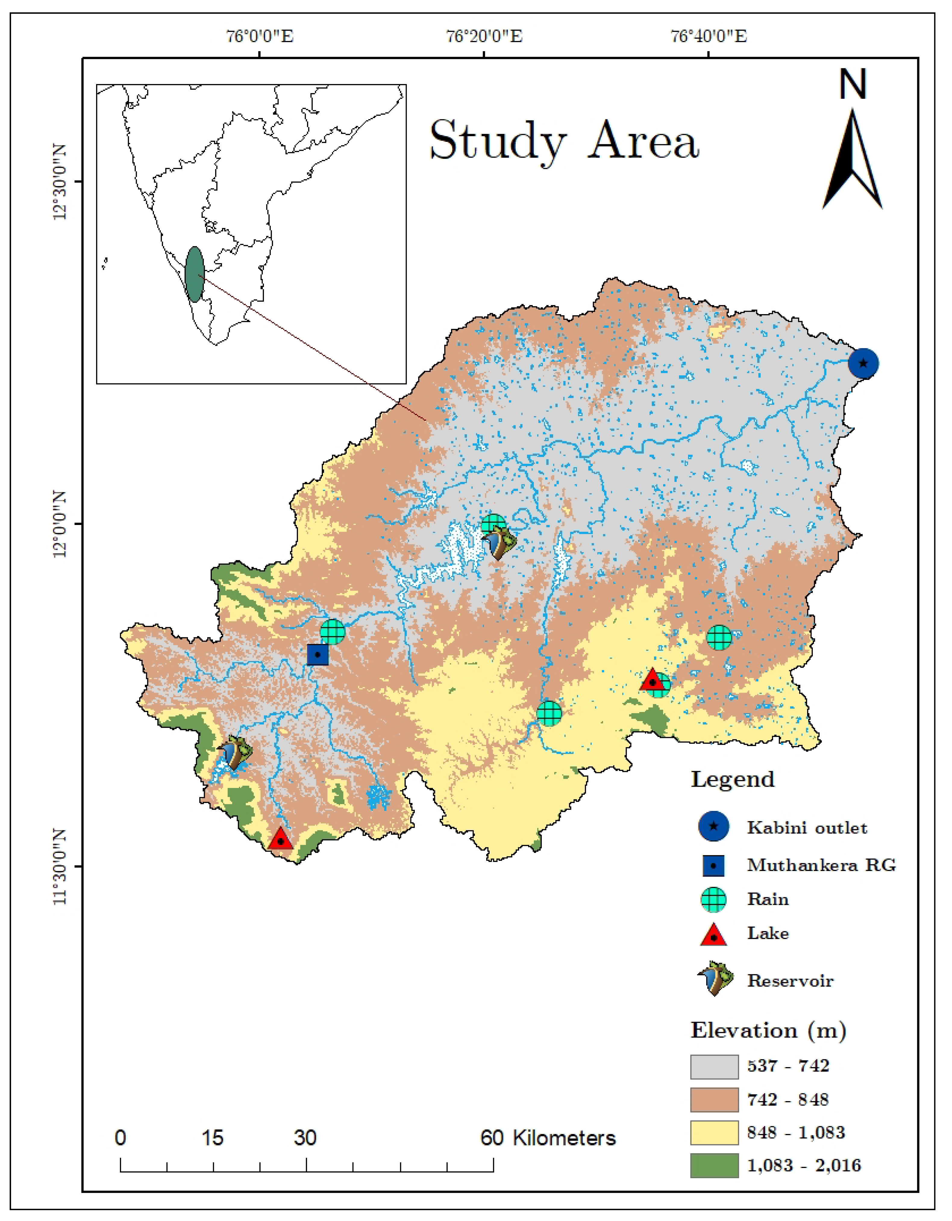
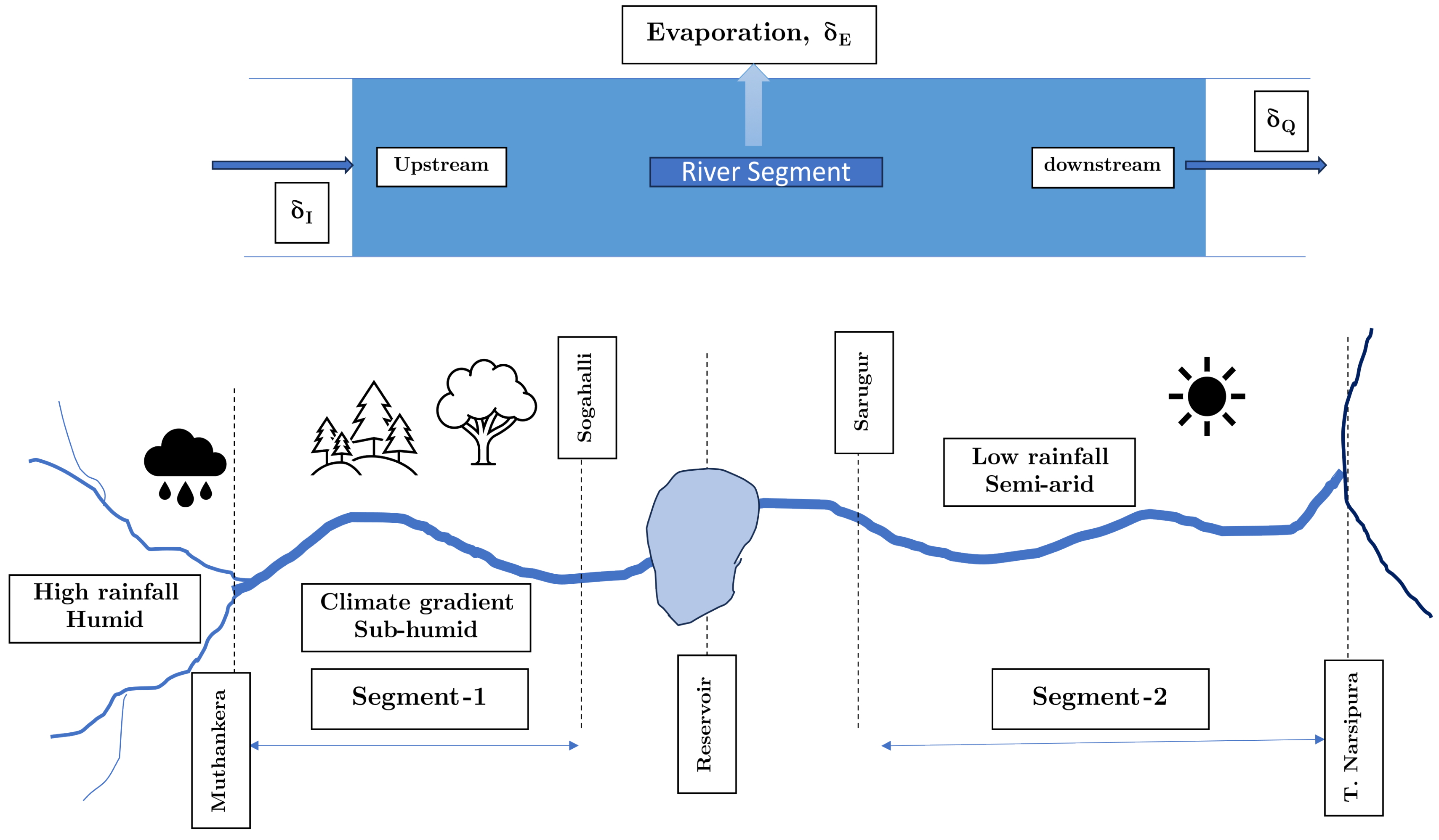
As shown in Figure 1, this study focuses on a selection of surface water bodies (lake and river segments), which span a range of climatic domains from humid and semi-arid, and each possessing unique characteristics (Table 1).
The first site, Berambadi lake (), also known as the tank, is located in the Berambadi catchment, which spans an area of 84 and is part of the Kabini Critical Zone Observatory in the southern part of Karnataka [13,14,15]. The Berambadi lake is a perennial body of water and the largest among the small to medium-sized ephemeral tanks located in the Berambadi catchment area. Pookode Lake, Kerala’s freshwater lake covering an area of , presents contrasting environment to Berambadi lake [16]. As the origin point of the Panamaram River, this lake experiences both southwest and northeast monsoons, creating varied conditions for evaporation studies.
Our study focuses on two distinct segments of Kabini river, each providing unique environmental conditions and rich data for examining evaporation dynamics. The first segment extends from Muthankera to Sogahalli (upstream of the Kabini reservoir). It lies within a humid to sub-humid climate gradient and hosts a hydrological observation station operated by a Central Water Commission (CWC) at Muthankera. The second river segment under our study is located at Sarugur, downstream of the Kabini reservoir, extending to T. Narsipura. Its semi-arid climatic domain offers a contrast to the humid conditions of the first segment. Together, the diverse sites included in the study provide a comprehensive perspective on the evaporation dynamics across two types of surface water bodies and climatic domains.
Figure 1.
Study Area
3. Materials and Methods
3.1. Fieldwork and sampling collection
This study relies on samples collected during three distinct seasons: pre-monsoon, monsoon, and post-monsoon in 2018. For the Berambadi lake and Pookode Lake, we focused on the central section for the sample collection. In the case of river water sampling, we made an assumption of thorough water mixing due to turbulent flow, which effectively mitigates potential isotopic enrichment on the water surface. To ensure a representative sample, water was collected 0.6m below the water surface. The timing of sampling was thoughtfully coordinated to align with the flow velocity of the river. This approach ensures the collection of homogenous original water, minimising the influence of temporal turbulence of headwater isotopes on our estimation results. Consequently, by calculating the flow velocity, downstream sampling was strategically scheduled between 12 to 36 hours after the initial upstream collection. In reservoirs, the isotope signature of the upstream flow to the reservoir is considered as the inflow isotope signature. On the other hand, the water that is released from the dam or reservoir is considered to have the outflow isotope signature during monsoon or peak flow conditions. However, during dry periods when water is not released from the dam due to low flow, the reservoir’s water samples are considered to reflect the outflow isotope signature.
Rainwater samples were collected from five distinct locations (RC1, RC2, RC3, RC4, RC5) during 2017-2019, each chosen with the aim of providing as broad a spatial coverage as possible, in an effort to capture a comprehensive picture of the landscape’s variability and climate. The specific locations took into account the local land use and land cover (LULC) (Refer to Figure 1). Sampling intervals were approximately every two weeks, although this varied slightly depending on the occurrence of rainfall events. The collection of rainwater samples was carried out using a simple collector that we developed in-house, which aligns with the standard guidelines of the International Atomic Energy Agency (IAEA) and the Global Network of Isotopes in Precipitation (GNIP). This collector employed a totalizer with a tube and a "dip-in" design. The design is particularly suited to India’s climate as it minimizes evaporation, thus preserving the integrity of the samples [15,17]. With this rigorous approach, we ensured that our rainwater samples were representative and reliable for our analysis.
Groundwater samples were obtained from both the humid and semi-arid sub-catchments, with the intent to characterize the isotopic signatures of the baseflow feeding into the inflowing water bodies. However, due to the challenging accessibility of the terrain, no groundwater samples could be gathered from the transition zone. Notably, the method of sample collection varied with the terrain and water availability. In the humid sub-catchment, where groundwater is often found near the surface, samples were drawn from dug wells. Conversely, in the semi-arid sub-catchment, the need to access deeper groundwater necessitated the use of bore or tube wells [15,18]. These varying collection methods not only reflect the distinctive characteristics of each sub-catchment but also have a bearing on the interpretation of the isotopic signatures, due to their influence on the depth and nature of the groundwater source.
In order to minimise the effects of isotopic fractionation caused by sunlight, we employed a meticulous water sampling method for stable isotopic measurements ( and ). Polypropylene bottles, each with a capacity of 60 ml, were pre-cleaned and used to collect the water samples. Prior to filling, these bottles were rinsed twice on site to minimize contamination. To preserve the integrity of the samples during transit to the laboratory for isotopic analysis and to prevent contamination, leakage, condensation, or evaporation, the filled bottles were sealed tightly with Parafilm sealing film [19]. Each sample’s specific location was recorded using a handheld GPS device, and it was further identified with a unique ID name, location name, and collection date. In addition, the sample bottles were labelled with the name of the collection site for easy identification. This thorough approach to sampling ensured that the isotopic measurements were as accurate and consistent as possible.
During each field campaign, in-situ water sample parameters such as temperature, electrical conductivity (EC), and pH were carefully recorded. Concurrently, all the collected samples underwent analysis for stable isotopes, specifically and . These combined efforts enabled a comprehensive understanding of the water’s physical properties and isotopic composition, ultimately providing essential information for the E/I ratio estimation.
3.2. Data sources
Monitoring of the basin’s hydrology has been ongoing since 1974, with data collection duties undertaken by the Central Water Commission (CWC) at Muthankera and by the Karnataka Water Resources Department at the Kabini dam. From these sources, we have gathered daily discharge data, measured in cubic meters per second (m3/s). Further, we sourced daily temperature, relative humidity, and wind speed data from NASA’s Prediction of Worldwide Energy Resources (POWER) Data Access Viewer (https://power.larc.nasa.gov/data-access-viewer/). The amalgamation of these resources, both historical and contemporary, offers a comprehensive view of the basin’s hydrological patterns. This data proves invaluable in understanding the inflow/outflow dynamics that are integral to our current study.
3.3. Stable isotope analysis
The isotopic analysis for the collected samples was conducted at the Centre for Earth Sciences at the Indian Institute of Science (IISc) in Bangalore. This analysis used advanced equipment - a Thermo Scientific-Finnigan Gas-benchII and a Thermo Scientific-MAT 253TM isotope ratio mass spectrometer. The oxygen and hydrogen isotopic analyses were performed using the equilibration method [20] in which water samples are equilibrated in a chamber with CO2 and H2 respectively. To analyze oxygen isotopes, we transferred 200µL of water into a specialized vial. The water was then mixed with a gas mixture of 3% CO2 and 97% He for 20 hours. For hydrogen isotope analysis, the water was mixed with a different gas mixture of 3% H2 and 97% He for 80 minutes. A platinum catalyst was used to facilitate this process. This procedure ensured accurate isotopic data for my research.
Isotope ratios in the samples are denoted using the ‘’ notation and referenced relative to the Vienna Standard Mean Ocean Water (VSMOW). We used internal laboratory standards, specifically the OASIS-WWW as per [21], and OASIS-LDK as per [22], to confirm the accuracy and precision of the analysis. These standards have been calibrated against international water standards. To address the need for intra-batch calibration and drift correction, we used replicate samples of the standards and another internal lab standard, OASIS-VOULEP, in the sample batches. This approach aided in maintaining accuracy throughout the batch analysis process.
During the Covid-19 pandemic, the isotope ratio mass spectrometer at IISc was not operational. Consequently, the rainwater samples from our study area were dispatched to the Physical Research Laboratory (PRL) in Ahmedabad for stable water isotope analysis. At the laboratory, the water samples were processed and analyzed using a Delta V Plus isotope ratio mass spectrometer and Gas Bench II, operating in a continuous flow mode. We computed the and values of the samples, by methodologies specified by [23,24].
The instrumental precision both at IISc, as well as PRL (based on repeated measurements of multiple aliquots of each sample), was and for and , respectively.
3.4. LMWL and Bayesian linear regression model formulation for stable isotope data
The concept of a Local Meteoric Water Line (LMWL) is crucial to interpreting site-specific isotope data. Unlike the Global Meteoric Water Line (GMWL) [25,26], the LMWL takes into account regional factors, making it particularly valuable for locations where precipitation derives moisture from sources other than maritime ones [9].
In this research, we aimed to establish the Local Meteoric Water Line (LMWL), diverged from the traditional approach of using linear regression analysis, and instead adopted Bayesian regression analysis for our study area, using data gathered from the isotopic characteristics of rainwater samples collected during the period from 2017 to 2019. This was motivated by the fact that Bayesian methods offer an inherently probabilistic framework, thereby allowing us to integrate the intrinsic variability and uncertainty present in isotopic measurements more effectively. This way, we could derive a more substantial and representative LMWL for our area of study. Bayesian methods incorporate prior knowledge about parameters and combine it with data to make statistical inferences. This makes it especially suitable for complex environmental systems where data might be uncertain or sparse, providing a probabilistic framework that handles uncertainty comprehensively. In the context of our study, this allowed us to incorporate the inherent variability and uncertainty in isotopic measurements while determining the LMWL.
Bayesian inference is a statistical method that uses Bayes’ theorem to update the probability of a hypothesis after obtaining new evidence. The theorem states that the posterior probability of a hypothesis, given the evidence, is proportional to the product of the prior probability of the hypothesis and the likelihood of the evidence given the hypothesis.
This is the example of the Bayesian inference equation:
In the bivariate regression modeling to interpret the stable isotope data, specifically focusing on the statistical relationship between (the dependent variable ’y’) and (the independent variable ’x’). The fundamental equation for the model is expressed as:
where is the intercept, is the slope of the regression line, and is the residual error term. The residuals, , are normally distributed with a mean of 0 and an unknown standard deviation .
In terms of µ (the expected value of 2H), this can be reformulated as:
and is following a normal distribution parameterized by mean and standard deviation , denoted as: .
In a Bayesian framework, to infer the posterior distributions of the parameters , , and given the observed and values. The prior beliefs about these parameters are updated using the likelihood, which is determined by how well our model, parameterized by , , and , predicts the observed values for the given values.
In formulating our model, we assigned each parameter a prior probability distribution that encapsulates our initial beliefs about these parameters before observing any data. The intercept and slope are assigned normal distributions centered at zero with a standard deviation of 20 (), reflecting our non-informative priors due to the lack of strong initial knowledge about these parameters. Similarly, we assigned a HalfNormal distribution to the standard deviation of the error term, , appropriate for strictly positive parameters.
The likelihood of the observed data given the parameters is then expressed as follows:
That is, given the parameters , , and , the values are normally distributed around the mean value with a standard deviation .
The posterior distribution, representing the updated beliefs about the parameters after observing the data, can be obtained by applying Bayes’ theorem. Using equation2,
In Appendices Figure A1 and Figure A2 demonstrates the complex interplay between the data, likelihood, parameters, and priors in the Bayesian framework applied in this study. Figure A1 visualizes the convergence of our MCMC chains, a key marker of the reliability of our sampling process. Figure A2 illustrates the intricate relationships between parameters, providing potential correlations.
3.5. Calculation fraction of evaporation
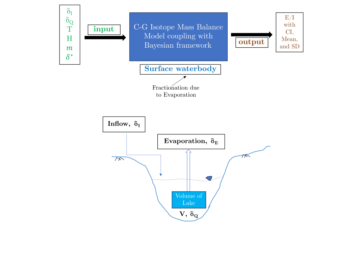
The Isotope Mass Balance (IMB) technique requires the collection of multiple types of data to evaluate water balance accurately. This includes information on the and composition of surface water, climatology measurements such as precipitation, temperature, relative humidity, and evaporation, geographic data like water body and watershed area, and isotopic compositions of precipitation and water vapor. These data points are essential to provide a detailed characterization of site-specific hydrology. The Isotope Mass Balance (IMB) model assumes that the water body being studied is well-mixed and that steady-state conditions are present [2,11,27,28,29].
The Isotope Mass Balance (IMB) technique is utilized to determine evaporation/inflow rates by analyzing the isotopic difference between the evaporatively enriched surface waterbody, such as lakes, and rivers, and the precipitation input. For a well-mixed surface water body that is in an isotopic and hydrologic steady state, the annual water balance and isotope balance can be expressed as [7,30,31]:
Mass balance of a waterbody at a hydrologic steady state (kept at a constant volume while undergoing evaporation with liquid outflow),
where V is the volume of the water body, I is the rate of inflow from the various sources, E is the rate of evaporation, and Q is the rate of outflow.
The analogous isotope mass balance equation using stable water isotope tracer ( or ):
where is the isotopic composition of inflow, is the isotopic composition of outflow, is the isotopic composition of evaporation flux, and is the isotopic composition of water undergoing evaporation in ‰.
Using equations 8 and 9, the Evaporation to Inflow ratio (E/I) can be obtained as,
Waterbodies can receive water from various sources such as precipitation that falls directly onto the surface of the water, as well as surface and subsurface runoff (groundwater) from surrounding areas. Additionally, they can also receive water from upstream water bodies that flow into them [11].
Here, P, S, G, and U are Precipitation on the waterbody, surface runoff, groundwater, and inflow from upstream respectively. is the isotopic composition of component x. In the context of a well-mixed waterbody, it is commonly assumed that the isotopic value of the outflow is approximately equal to the isotopic value of the waterbody itself [7,31] (), because no isotope fractionation occurs. While it is relatively straightforward to obtain , , , and through sampling and analysis, determining the value of is a more complicated process. In the context of a well-mixed waterbody, the isotopic composition of the water that is lost due to evaporation can be obtained based on the [7,32] and modified by [10,11,29] to use water isotope data in the per mil notation.
where,
For
Here, T is the temperature given in Kelvin degrees.
is the limiting isotope enrichment factor. The process of isotope enrichment during evaporation of surface water is influenced by various physical and meteorological conditions, which determine the rate and extent of the enrichment. However, there is a limit to this process, known as the "limiting isotope composition ( )", beyond which further evaporation does not result in any more isotope enrichment [5].
3.6. Bayesian Estimation of Evaporative Loss: Integration with the Craig-Gordon Model
Estimating evaporative loss in water bodies is an intricate process, with several parameters contributing to the complexity [34,35]. These parameters include the isotopic composition of inflow water (), the isotopic composition of outflow water (), the Evaporation to Inflow ratio (E/I), the enrichment slope (m), and the limiting isotope enrichment factor (). Each of these parameters carries an inherent level of uncertainty because they depend on meteorological parameters like temperature, humidity, and wind speed [2,10,35,36]. In traditional approaches, these parameters are treated as point estimates, which may not fully represent their inherent variability and uncertainty. However, a Bayesian approach offers an effective way to handle this by producing entire distributions of possible values for these parameters [37]. This probabilistic approach allows us to account for uncertainties in a natural and integrated manner, providing a more comprehensive understanding of the parameter space.
The Bayesian framework leveraged prior knowledge or assumptions about the parameters, expressed in the form of prior distributions as formulated in equations 1 and 2. In cases of isotopic composition of inflow water, and isotopic composition of outflow water, specific knowledge about these parameters is available from current studies, this information is directly incorporated into the analysis, enhancing the robustness of our inference. Alternatively, in situations, Evaporation to Inflow ratio (E/I), little or no specific prior knowledge is available, and non-informative priors are used. These priors have minimal impact on the results, thereby ensuring that the observed data primarily influence the posterior distributions. Further, Bayesian methods, specifically Markov Chain Monte Carlo (MCMC) methods, have the flexibility to handle complex models that may not be analytically tractable [38,39,40]. They can work with virtually any form of likelihood and prior, enabling the application of more realistic models to the data. This characteristic makes Bayesian methods particularly suitable for integrating with the Craig-Gordon model, a well-established theoretical framework in hydrology.
The equation 16 can be formulated as:
It is a modification of the Craig-Gordon model, adapted to suit the Bayesian framework. This model offers a more in-depth understanding of the system [37]. In this version, represents the final stable isotope composition () of the partially evaporated outflowing water from a waterbody. The parameters in the equation are as follows:
- is the initial stable isotope composition () of the inflowing water.
- r signifies the evaporated fraction (E/I), the estimation of which is our primary objective.
- A corresponds to the parameter m in the Craig-Gordon model.
- D is the limiting isotopic enrichment due to evaporation.
The parameters A and D are calculated using equation 17 and 18 respectively.
The prior distributions for the parameters in the model are, r (Evaporated Fraction (E/I)): The prior for r is specified as a Uniform distribution that has equal probability density for all values between the lower and upper bounds. In this case, these bounds are 0 and 1, reflecting our assumption that the evaporated fraction could be any value between 0 and 1 with equal likelihood.
The prior distributions for the parameters in the model are,
- r (Evaporated Fraction (E/I)): The prior for r is specified as a Uniform distribution that has equal probability density for all values between the lower and upper bounds. In this case, these bounds are 0 and 1, reflecting our assumption that the evaporated fraction could be any value between 0 and 1 with equal likelihood.
- (Initial Stable Isotope Composition ()): The prior for is a Normal distribution with mean equal to the observed value of and standard deviation equal to the uncertainty in .
- A (Parameter m in Craig-Gordon model): The prior for A is a Normal distribution with mean equal to the pre-calculated A value and standard deviation equal to the uncertainty in A.
- D (Limiting Isotopic Enrichment ()): The prior for D is also a Normal distribution with mean equal to the calculated D value and standard deviation equal to the uncertainty in D.
Here, U denotes a Uniform distribution and N denotes a Normal distribution. In the case of the Normal distribution, the first argument is the mean and the second is the standard deviation. These prior distributions reflect our assumptions about the parameters before seeing the data, based on pre-existing knowledge or uncertainty.
The likelihood is a function that measures the goodness of fit of the model to the data. It calculates the probability of observing the data given the parameters of the model. In this case, the likelihood function is specified as a Normal distribution, reflecting the assumption that the observed and values for the waterbody (the ’data’) vary around the model-predicted values (’ ’ parameter) according to a normal distribution with standard deviation equal to the measurement uncertainties.
Here, are the standard deviations (uncertainties) in the observed values.
The posterior distribution is the probability distribution that represents updated beliefs about the parameter after having seen the data. In the context of this model, we have a multivariate posterior distribution, because we are updating our beliefs about multiple parameters (, A, D, and r) simultaneously. The posterior distribution can’t usually be written down in a simple form like the prior or likelihood because it involves a complicated integral over all the parameters in the model.
This represents that our beliefs about the parameters , A, D, and r given the observed data and the uncertainties , are represented by the set of samples produced by the Hamiltonian Monte Carlo (HMC) algorithm.
4. Results & Discussion
4.1. Rainwater stable isotopes
This study examined a three-year (2017 to 2019) values of stable isotopes in rainwater collected from various locations within the catchment as detailed in Figure 1, Table 2. The stable isotopes in precipitation exhibited considerable variation, with ranges of to for , to for , and to for d-excess across 105 observations. The standard deviations for these isotopes were , , and respectively. The weighted averages for , , and d-excess were , , and respectively, illustrating the central tendency of the data. These values reflect the complex interplay of various atmospheric like rainfall amount decreasing, the temperature increasing and humidity decreasing along the downstream of the catchment, geographical like RC3 located in forest cover, RC2 located in the agricultural farm, RC1 located in an urban area, RC4 near to reservoir and RC5 is in a humid rural area and climatic factors like humid to semiarid climatic gradient along the river segment that influence the isotopic composition of precipitation in the region.
To interpret these variations and construct a Local Meteoric Water Line (LMWL), a Bayesian approach to linear regression model was employed as demonstrated in Equation 3. This approach enabled the integration of prior information about the parameters into our model, thus allowing a more comprehensive analysis than traditional linear regression, which solely maximizes the likelihood function as provided in equations 2 and 4. The Bayesian approach uses Bayes’ theorem to combine the likelihood function with prior distributions for the parameters, leading to a posterior distribution for the parameters (Eq7).

Table 2.
Statistical Summary of Seasonal Variation in Rainwater Isotope Composition and d-excess Values at Five Different Locations (RC1-RC5)
Table 2.
Statistical Summary of Seasonal Variation in Rainwater Isotope Composition and d-excess Values at Five Different Locations (RC1-RC5)
| Location | Season | n | d-excess | |||||||||||
|---|---|---|---|---|---|---|---|---|---|---|---|---|---|---|
| Min | Max | Avg | SD | Min | Max | Avg | SD | Min | Max | Avg | SD | |||
| RC1 | M | 11 | -5.2 | 2.2 | -0.92 | 2.3 | -31 | 27.3 | 1.01 | 19.21 | 3.2 | 10.5 | 8.4 | 2.32 |
| RC1 | Post-M | 4 | -6.3 | -3.5 | -4.41 | 1.24 | -40.4 | -20.3 | -25.41 | 8.61 | 3 | 10.9 | 9.75 | 3.73 |
| RC1 | Pre-M | 1 | 2.3 | 2.3 | 2.3 | 27.8 | 27.8 | 27.8 | 9.8 | 9.8 | 9.8 | |||
| RC2 | M | 20 | -5.5 | 3.6 | -1.91 | 2.2 | -39.2 | 38.7 | -6.64 | 18.52 | 3.1 | 13.1 | 8.54 | 2.64 |
| RC2 | Post-M | 11 | -7.7 | -0.8 | -5.23 | 1.98 | -50.6 | 4.1 | -31.41 | 15.11 | 2.8 | 14.8 | 10.43 | 2.95 |
| RC2 | Pre-M | 6 | 1.3 | 4.4 | 2.43 | 1.36 | 14.7 | 44.5 | 26.51 | 12.86 | 0.2 | 10.4 | 7.11 | 3.83 |
| RC3 | M | 7 | -5.1 | 1.8 | -0.31 | 2.33 | -37.3 | 24.1 | 4.03 | 20.88 | 3.1 | 10.1 | 6.66 | 3.31 |
| RC3 | Post-M | 4 | -7.1 | -3.3 | -5.17 | 1.62 | -51.2 | -15.3 | -33.4 | 14.93 | 5.9 | 10.8 | 8.01 | 2.3 |
| RC3 | Pre-M | 2 | 1.5 | 2.3 | 2.1 | 0.57 | 14.1 | 24.7 | 22.05 | 7.5 | 2.1 | 6.1 | 5.1 | 2.83 |
| RC4 | M | 6 | -3.6 | 0.4 | -0.79 | 1.47 | -23.5 | 14.8 | 1.01 | 13.87 | 2.7 | 11.8 | 7.45 | 3.9 |
| RC4 | Post-M | 4 | -4.3 | -0.2 | -2.6 | 1.89 | -27.6 | 8.4 | -15.17 | 16.38 | 0.5 | 11 | 5.51 | 4.9 |
| RC4 | Pre-M | 1 | -0.8 | -0.8 | -0.8 | 2.1 | 2.1 | 2.1 | 8.6 | 8.6 | 8.6 | |||
| RC5 | M | 21 | -6 | 1.2 | -1.25 | 1.91 | -39.7 | 19.4 | -2.21 | 14.38 | -0.2 | 11.2 | 7.82 | 3.47 |
| RC5 | Post-M | 7 | -8 | 0 | -5.24 | 3.2 | -61.5 | 10.2 | -34.11 | 27.19 | 2.6 | 13.1 | 7.73 | 3.72 |
| n: no. of samples; Max: maximum; Min: minimum; Avg: weighted average; SD: standard deviation; M: monsoon. | ||||||||||||||
After implementing Bayes’ theorem, we derived the posterior distribution of the parameters, distinct from traditional maximum likelihood estimation which seeks a singular optimal value per parameter. The Bayesian approach, conversely, yields a complete distribution for each parameter as shown in Figure 2 and Figure 3. This full distribution encapsulates information from the observed data through the likelihood, and our prior beliefs through the priors. We attained this by utilizing the No-U-Turn Sampler (NUTS), a variant of the Hamiltonian Monte Carlo (HMC) algorithm [41,42]. The application of NUTS algorithm was executed in PyMC3 [43], where we initiated four chains for each parameter, generating 5000 samples per chain following a tuning period of 1000 iterations. These samples provided a representation of the posterior distribution, aiding our inference on the parameters given the data. Upon completion of the sampling process, we examined the NUTS sampler’s output to estimate the posterior distributions of the parameters. Utilizing a methodology that combines non-informative priors, Bayesian linear regression, and the NUTS sampler enabled us to estimate the parameters and their associated uncertainties (Table 3). This process helped to provide the underlying relationship between and . Our approach showcases the potential of Bayesian methods to integrate prior information with observed data to yield a probabilistic framework that accommodates uncertainty and complexity inherent in environmental data analysis.
The posterior plots as shown in Figure 2 and Figure 3, served as instruments for the visualization of uncertainties intrinsic to our model parameters, thereby enabling the decision-making process. Each plot manifests the probability distribution of parameters - the Intercept, Slope, and Sigma - as obtained through probability sampling. These distributions illustrate a full range of potential values for each parameter, conditioned by the interplay of the observed data of and , prior information (, ), and the likelihood function (Eq. 6). The ensuing figures demarcated the 68% and 95% Highest Density Intervals (HDIs) for each parameter. These intervals, also known as credible intervals, highlight the most probable parameter values given our data and model. For instance, the intercept has a mean value of 7.90, with a 68% HDI from 7.54 to 8.25 and a 95% HDI from 7.19 to 8.62. Similarly, the slope has a mean of 7.89, with a 68% HDI from 7.79 to 8.00 and a 95% HDI from 7.68 to 8.10. Finally, the sigma parameter has a mean of 3.13, with a 68% HDI from 2.91 to 3.31 and a 95% HDI from 2.72 to 3.53 as tabulated in Table 3. These quantitative insights offer clear representations of parameter uncertainties, enabling us to build a more rigorous understanding of the and relationship.
Table 3.
Bayesian Linear Regression Estimates for Predicting Stable Water Isotopes from Rainfall
| Parameter | Mean | SD | 68% HDI (16% - 84%) | 95% HDI (2.5% - 97.5%) |
|---|---|---|---|---|
| Intercept | 7.90 | 0.36 | 7.54 - 8.25 | 7.19 - 8.62 |
| Slope | 7.89 | 0.11 | 7.79 - 8.00 | 7.68 - 8.10 |
| Sigma | 3.13 | 0.21 | 2.91 - 3.31 | 2.72 - 3.53 |
These model parameters for the intercept and slope, including their uncertainties, were incorporated into the equation for the Local Meteoric Water Line (LMWL). For the 68% Highest Density Interval (HDI), which represents a range of values that contain 68% of the posterior distribution and are most credible, the equation for the LMWL becomes:
For the 95% HDI, which encompasses 95% of the posterior distribution and thus a wider range of credible values, the LMWL is given by:
In the plot (Figure 4), we presented a comprehensive visualization of the Kabini catchment’s local meteoric water line, drawn using Bayesian regression model parameters for the 68% credible interval. The and findings align with the principle of isotopic fractionation, highlighting a consistent overall trend in the data. This also offered an intricate understanding of how isotopic compositions in various water sources–lakes, rivers, reservoirs, and groundwater–could differ across different seasons and climatic conditions, contributing significantly to the field’s understanding. These are effectively depicted by the different colors and markers in the plot. For instance, the groundwater data points, shown in purple, depicted a distinct trend compared to other water bodies, indicating unique isotopic behaviors due to factors such as evaporation rates, water source, and water-rock interactions. The markers’ styles and fill-colors represented climatic conditions (Humid vs. Semi-arid) and seasonal timing (Pre-Monsoon, Monsoon, and Post-Monsoon), each demonstrating a unique pattern, suggesting that these factors also influence the isotopic compositions of water bodies.
4.2. Ground water stable isotopes
In the current study, the groundwater stable isotopes were examined in two distinct climate domains: Semiarid and Humid, over different seasons. The pH values indicated relatively neutral groundwater in both climates, varying from slightly acidic to mildly alkaline. Specifically, the Semiarid climate domain revealed a pH range of 6.6 to 7.1, with a mean value of around 6.9. In contrast, the Humid climate exhibits a higher pH range, from 7.4 to 8, with an average of approximately 7.6. In terms of Electrical Conductivity (EC), a measure of the dissolved mineral content, a significant discrepancy was observed between the two climatic zones. The Semiarid climate reflected EC values spanning from to , which is higher compared to the Humid climate’s range between and as shown in Figure 5. This significant difference implies a larger mineral content in the Semiarid climate’s groundwater, a common phenomenon in arid and semiarid regions, potentially attributed to lesser rainfall volumes or unique geological composition of the terrain [44]. An important aspect to consider here is the depth of the groundwater source. In this study, the groundwater samples from the Semiarid climate were obtained from deep aquifers, whereas those from the Humid region were from shallow aquifers. This difference in source depth could also be a contributing factor to the substantial divergence observed in the EC values between the two climatic zones. The minerals dissolved in groundwater can originate from the interaction with the surrounding rocks and soils, and deeper aquifers have more residence time for these interactions, potentially leading to higher mineral contents.
The range of values is from -3.76‰ to -1.9‰, while spans from -24.21‰ to -5‰. Interestingly, these values are generally more negative in the Semiarid climate domain. This observation could be attributed to the fact that the Semiarid region in the current study, being farther from coastal rainfall sources, receives lighter rainfall [44,45]. Additionally, the Semiarid region in this study typically experiences post-monsoon rainfall, whereas the Humid region sees minimal or no rainfall in this season. The d-excess values, computed from and , offered valuable information about the initial humidity conditions during the evaporation process. The values within the dataset ranged from 3.95‰ to 12.58‰, with the Humid climate domain typically exhibiting higher d-excess values, indicative of higher humidity at the onset of evaporation.
4.3. Isotope behavior and E/I dynamics in lake water
Berambadi and Pookode lake are considered for analysis in semiarid and humid climate to understand the evaporation to inflow pattern in the study area. Berambadi, in a semi-arid climate, shows a varying range of and from 8.6‰ and 44.2‰ to -4.4‰ and -26.9‰, respectively. The d-excess value, which is a sensitive indicator of evaporative conditions, also fluctuates significantly from -24.79 to 8.3. This can be attributed to high evaporation rates typically observed in semi-arid regions, leading to enriched heavier isotopes in the residual water. The pH ranges from 6.55 to 8.8, reflecting varying levels of acidity and alkalinity. High values can indicate higher alkaline levels, possibly due to the higher evaporation leaving behind minerals. The electrical conductivity (EC), indicative of the water’s total dissolved solids (TDS), varies from 159 S/cm to 567.1 S/cm. This wide range suggests significant temporal variability in the dissolved content of the water. Pookode, classified under a humid climate, exhibits a different isotopic pattern compared to Berambadi. The range of and is from 1.9‰ and 10.0‰ to -3.2‰ and -12.6‰, respectively. Unlike Berambadi, the d-excess values remain relatively positive, ranging from -5.2 to 13‰, indicating less evaporation impact. The pH varies from 6.4 to 7.2, showing a lesser range than Berambadi, suggesting more stable conditions. Similarly, EC is significantly lower than Berambadi, ranging from 50.6 S/cm to 65.6 S/cm, pointing towards lower TDS in the water, which could be expected due to less evaporation under humid conditions.
The contrasting isotopic behaviors observed between Berambadi and Pookode are related to their distinct climatic conditions. The higher range of isotopic values and d-excess in Berambadi could be attributed to the intense evaporation in a semi-arid environment that results in significant enrichment of heavier isotopes and variable d-excess. On the other hand, Pookode, situated in a humid climate, has lower and more stable isotopic values. The relatively stable and positive d-excess values, along with lower EC, indicate less evaporation, which is characteristic of a humid climate. Furthermore, the changes in isotopic values over the seasons in both locations may suggest the impact of the monsoon season, with the pre-monsoon months generally showing more enriched isotope values due to stronger evaporation, and the monsoon and post-monsoon months showing more depleted values due to input from rainfall as tabulated in Table 4.
The mass balance of a lake in a hydrologic steady state maintained at a constant volume while experiencing evaporation and water outflow is expressed through equations 8 and 9. The inflow into the lake can be broadly classified into surface runoff and baseflow. The stable isotopes for these components are derived from different sources: for surface water, precipitation is considered, while groundwater isotopes that are sampled and analysed during the study are taken for baseflow. The fraction of each component that contributes to the stream flow is estimated using Electrical Conductivity (EC). Our calibration across the three seasons of 2018 - Pre-Monsoon, Monsoon, and Post-Monsoon exhibits considerable seasonal fluctuations in the evaporation-to-inflow (E/I) ratios for both Hydrogen and Oxygen isotopes in the two lakes of study as shown in Figure 6. At Berambadi Lake during Pre-Monsoon, the high E/I using and are 0.460 and 0.440 readings indicate a larger amount of evaporation compared to inflow. This could be a result of hotter, drier conditions of semiarid climate with surface water temperature approximately 32°C leading up to the monsoon, enhancing evaporation rates. Consequently, the isotopic concentration in the lake water increases. In the Monsoon season, the drastic drop in E/I using both and are 0.247 and 0.172 can be attributed to heavy rainfall. As monsoonal inflow outpaces evaporation, it dilutes the isotopic concentration in the water, thus reducing the E/I ratios. During the Post-Monsoon period, the increased in E/I 0.388 and 0.254 denote a resurgence in evaporation rates. As the influx of monsoonal water decreases, and drier conditions resume, evaporation rates pick up, once again enriching the isotopic concentration in the water.
At Pookode Lake during the Pre-Monsoon conditions, a similar trend as observed in Berambadi is evident, with E/I values at 0.415 and 0.259 using and respectively. The elevated evaporation rates reflect a drier climate ahead of the monsoon. In the Monsoon season, there is an even more significant drop in E/I, with and values being 0.147 and 0.066 compared to Berambadi. This could be a consequence of higher rainfall, possibly due to the geographical and climatic conditions of Pookode as shown in the study area map and Table 1. During the Post-Monsoon period, Pookode records E/I values of 0.185 and 0.115, which are lower compared to Berambadi. This less pronounced increase suggests a slower return to drier conditions, possibly influenced by factors such as local climate, vegetation, soil conditions, or topography. These findings underscore the importance of considering seasonal variations when studying evaporation dynamics. Additionally, they indicate that even within the same broad climatic region, local variations in climate and other environmental factors can significantly influence evaporation dynamics, as evidenced by the differences between the Berambadi and Pookode lakes.
Figure 6.
Seasonal Variation of Evaporation to Inflow Ratios (E/I) for and in the Lakes of Berambadi and Pookode.
Figure 6.
Seasonal Variation of Evaporation to Inflow Ratios (E/I) for and in the Lakes of Berambadi and Pookode.
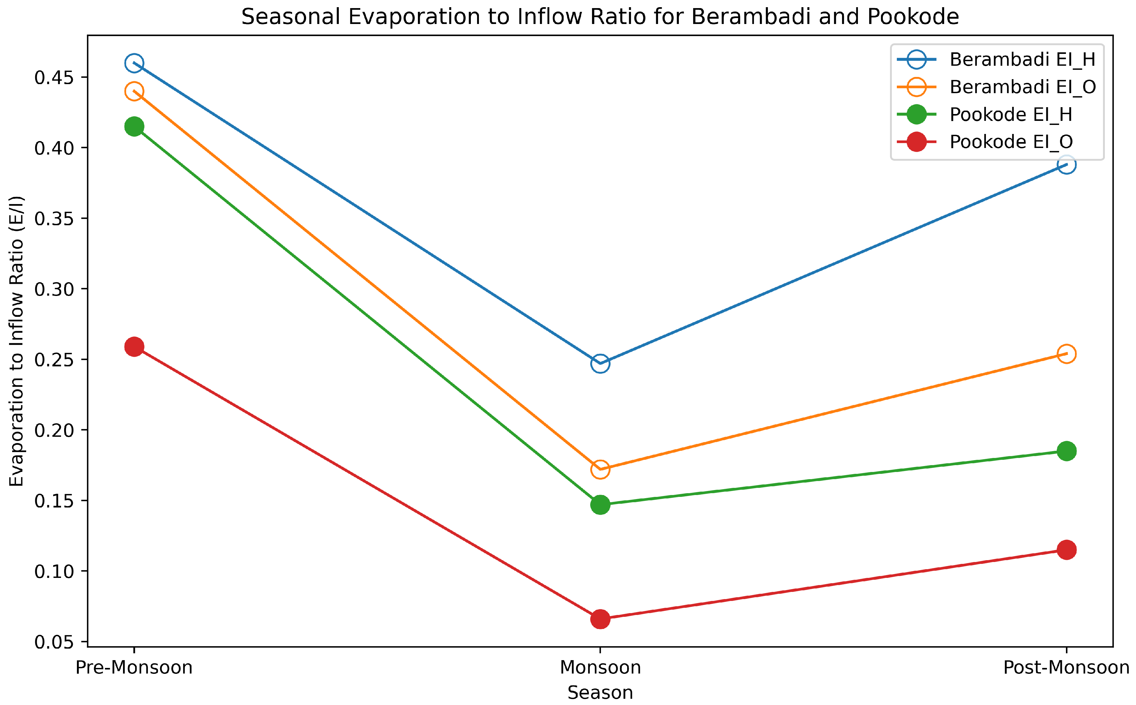
The Evaporation to Inflow (E/I) ratios for both and isotopes exhibited seasonal variations, indicating the dynamics of water loss due to evaporation relative to the input from inflows such as precipitation, groundwater, and surface run-off as shown in Figure 6. Both locations - Berambadi and Pookode - demonstrate higher E/I ratios in the pre-monsoon season, suggesting a greater degree of evaporation due to warmer temperatures and relatively lower humidity, which then decrease during the monsoon. The monsoon brings an influx of water and lower temperatures, which are likely causing the E/I ratios to decrease. Post-monsoon, we see a moderate rise in the E/I ratios, likely due to decreasing inflow and increasing evaporation as temperatures start to rise again. This pattern likely reflects changes in the balance of evaporation and inflow over different parts of the year, associated with monsoonal rainfall patterns. For both locations and across all seasons, the E/I ratio of is consistently higher than that of . This is in line with the known fractionation characteristics of water molecules during evaporation, where lighter isotopes (like ) are more likely to evaporate than heavier ones (like ) [4,46,47]. This fractionation is also temperature dependent, and it can provide insights into the temperature conditions at the time of evaporation.
The data also reveals some spatial differences. Across all seasons, Pookode demonstrates lower E/I ratios compared to Berambadi. This might suggest a higher proportion of inflow to evaporation at Pookode, possibly due to differences in humid and semiarid climate domain, higher rainfall amount, less resident time of ground water inflow to the humid lake and geographic conditions like near to western ghat region between the two sites. The E/I ratios provide clues about the potential sources of inflow to these lakes. Lower E/I ratios (as seen during the monsoon) could indicate a larger proportion of ’new’ water from precipitation or surface runoff entering the lake, which dilutes the lake’s existing water and reduces the E/I ratio. Conversely, higher E/I ratios (as seen pre-monsoon) could suggest a larger proportion of the lake’s water is ’old’ or ’residual’ water that has undergone significant evaporation, with relatively less ’new’ water entering the system.
The influence of surrounding vegetation and human activities also played keyrole. In case of Pookode lake, vegetation around the lake is reducing evaporation by providing shade and reducing wind speed at the lake surface. Meanwhile, in Berambadi lake, human activities such as water extraction for irrigation and drinking water supply, are significantly altering the inflow-outflow balance, impacting the E/I ratios. Also, human-induced changes in the catchment, such as deforestation or urbanization, can change the surface runoff characteristics, affecting the quantity and timing of inflow into the lake.
4.4. Stream water Isotope variations and calibration of E/I
This study of the Kabini River’s isotopic variation, from its origin in a humid climate zone (Segment-1) to a transition zone with semi-arid conditions (Segment-2), reveals intriguing seasonal and spatial variations. The pH levels of both segments largely maintain a near-neutral range across all seasons. However, a slight increase is observed from the pre-monsoon to the post-monsoon season in Segment-2. This increase, from a pH of 8.13 to 8.26, possibly points to an increased alkalinity associated with the evaporative conditions typical of semi-arid regions, or inputs from the weathering of local alkaline geological features. The Electrical Conductivity (EC) shows a significant increase in Segment-2. The average EC in the segment-1 77.8 µS/cm to 292 µS/cm in segment-2, indicating an increase in the total dissolved ions in this semi-arid segment. This increase could be due to enhanced mineral dissolution or possibly from anthropogenic contributions. Temperature variations between the two segments reflect their different climatic settings. Segment-2 records higher temperatures compared to Segment-1, signifying the warmer climatic conditions characteristic of the semi-arid region.
The stable water isotopes and values offer unique insights. For Segment-1, the and values display isotopic depletion from the initial point (I) to the final point (F) during the post-monsoon season, transitioning from -7.5‰ to -4.2‰ for and from -1.3‰ to 0.1‰ for . This pattern could indicate the contribution of isotopically lighter monsoon rain combined with isotopic fractionation via evaporation in the humid climate zone. In contrast, for Segment-2, a significant isotopic enrichment is observed from the initial point (I) to the final point (F) during the post-monsoon season, increasing from -23.3‰ to -15‰ for and from -6.3‰ to -4.41‰ for . These trends potentially reflect the effect of evaporation, which is expected to be higher in the semi-arid climate of this segment, leading to a pronounced degree of isotopic fractionation.
Table 5.
Seasonal variations in pH, EC, T, h, and , in initial and final points of the Kabini River, from a humid (Segment-1) to semi-arid zone (Segment-2).
Table 5.
Seasonal variations in pH, EC, T, h, and , in initial and final points of the Kabini River, from a humid (Segment-1) to semi-arid zone (Segment-2).
| Season | Location | pH | EC | T | h | ||||||
|---|---|---|---|---|---|---|---|---|---|---|---|
| Pre-M | Segment-1 | 7.4 | 122.4 | 29.5 | 0.62 | 3.8 | 2.3 | 12.5 | 3.8 | 0.12 | 0.09 |
| M | Segment-1 | 6.4 | 28 | 23.4 | 0.89 | -3.3 | -2.2 | -0.5 | -1.6 | 0.03 | 0.01 |
| Post-M | Segment-1 | 7.1 | 83 | 26.8 | 0.83 | -7.5 | -1.3 | -4.2 | 0.1 | 0.06 | 0.06 |
| Pre-M | Segment-2 | 8.13 | 345 | 32.8 | 0.53 | 1.2 | 0.9 | 15.0 | 3.5 | 0.15 | 0.13 |
| M | Segment-2 | 7.8 | 232 | 25.8 | 0.79 | -5.5 | -2.9 | -1.5 | -2.1 | 0.05 | 0.04 |
| Post-M | Segment-2 | 8.26 | 299 | 23.9 | 0.71 | -23.3 | -6.3 | -15 | -4.41 | 0.09 | 0.07 |
Here, Electrical Conductivity (EC) in S/cm; Temperature(T) in °C; Relative humidity (h); in ‰; E is ratio.
The river segment’s mass balance, when maintained at a hydrologic steady state, is essentially at a constant volume, concurrently experiencing evaporation and water outflow. This balance can be drawn through Equations 8 and 9. The inflow into the river primarily consists of three major components: surface runoff, upstream flow, and baseflow. Each of these components possesses distinct stable isotope signatures due to their varied sources. Precipitation is the primary source for surface water, and the isotopic composition of upstream inflow and baseflow is determined by upstream samples and groundwater isotopes, respectively. The contribution of each of these components to the overall stream flow is estimated using the Electrical Conductivity (EC) value. The isotopic composition at the head of the river segment () serves as our initial point, and the isotope ratio within the river water () could incrementally ascend along with the E/I ratio. This suggests a potential evolution towards a limit of isotopic enrichment (), where progresses towards as the E/I approaches unity [34]. Nonetheless, in practical terms, reaching remains unfeasible due to the relatively minor evaporation from the river caused by its brief residence time, approximately two days for the Kabini river segments. Indeed, our key emphasis is on the initial evaporation enrichment, as indicated by the perceptible shifts in the river isotopes, specifically the transition from to . This progression offers important insights into the isotopic changes that the river undergoes along its course from its source to its destination, shaped by factors such as climate conditions and evaporation rate.
In Segment-1, situated in the humid climate zone, the E/I ratios during the Pre-Monsoon season are estimated as 0.12 and 0.09 based on and , respectively. As we progress to Segment-2 in the same season, which traverses a semi-arid climate, these ratios escalate to 0.15 () and 0.13 (). The increase of these ratios signifies a rise in evaporation rate attributable to the semi-arid conditions, and thus, a greater isotopic fractionation. Interestingly, we find that the E/I ratio estimated using is slightly higher than that obtained using , a pattern also observed in lake studies. This inconsistency in E/I ratio estimation from dual isotopes will be explored in subsequent sections.
Further, the E/I ratios for Segment-2 in a semi-arid climate zone stand at an increased level. This observation signals the substantial influence of evaporation on the river water’s isotopic makeup within this segment, predominantly during the Pre-Monsoon season. At this time, the E/I ratios reach a peak of 0.15 () and 0.13 (). These patterns endorse the hypothesis that climate plays a significant role in the isotopic composition of river water. As the river meanders from the humid headwaters (Segment-1) to the semi-arid downstream reaches (Segment-2), the role of evaporation intensifies, thereby causing higher E/I ratios and pronounced isotopic fractionation. This reinforces the intricate interaction between climate conditions and water isotopes in the shaping of a river’s hydrological signature.
4.5. Uncertainty Estimation in E/I Ratios using Bayesian Methods
The Craig-Gordon (C-G) model has indeed been a significant mathematical model in understanding physical processes, isotopic fractionation during water vapor evaporation [32,35,36,46]. However, inherent in its use are certain assumptions which, while simplifying the modeling process, may not fully capture the complex nature of the system. For instance, the C-G model assumes equilibrium between water vapor molecules and the water surface. It also assumes that the water molecules that have evaporated immediately intermix with the ambient air, thereby oversimplifying the effects of external factors such as wind.
In response to these limitations, the integration of Bayesian methods with the C-G model provides a more refined approach. The Bayesian framework allows us to systematize the quantification of uncertainty, facilitating a more comprehensive representation of the real-world scenario. It provides a mechanism to manage uncertainties in stable water isotopes, meteorological parameters, sampling errors and intricacies better, it does not alter the foundational physics encapsulated within the C-G model. Instead, it should be seen as a complementary methodology [?]. The Bayesian methods present a robust framework for deploying the C-G model in a complex, real-world context, thereby enriching its predictive capabilities and allowing us to understand more accurate and meaningful insights from our sampling data.
In this study, we opted to employ the No-U-Turn Sampler (NUTS), a variant of the Hamiltonian Monte Carlo (HMC), to draw samples from our Bayesian model’s posterior distribution (Equation 21). Given the multidimensional nature of our model with multiple input variables including isotopic values of inflow and outflow, the m and parameters which are influenced by meteorological parameters like temperature and humidity, and various uncertainties this algorithm can efficiently explore high-dimensional parameter spaces. The algorithm achieves this efficiency by leveraging gradient information from the likelihood function (equation 20) to guide its sampling trajectory. Secondly, NUTS carefully self-tunes during the initial warm-up phase, refining the step size and the number of steps to take in the simulation [41]. In our study, we have chosen to draw 5000 samples for each run. This quantity offered a balance between computational efficiency and the accurate estimation of the posterior distributions. The PyMC3 library provides a tuning phase, typically referred to as ’burn-in’ in the MCMC literature, the number of tuning steps considered in these simulations is 1000.
4.5.1. Lake
Bayesian modelling, employing the Hamiltonian Monte Carlo sampler methodology, has been utilized to calibrate uncertainties in the evaporation-to-inflow (E/I) ratios. The detailed results of this calibration, tabulated in Table 6, provide a thorough exploration of seasonality and location-specific differences. Two distinct sites, Berambadi and Pookode, were studied, with a focus on two isotopes: and . The metrics derived from this analysis, including the mean, median, standard deviation, and 68% and 95% confidence intervals, offer a comprehensive understanding of the E/I ratios, encapsulating the findings and their associated uncertainties.
Focusing on the site of Berambadi, we observe a mean E/I ratio of 0.43 in the pre-monsoon month of April. The minimal standard deviation of 0.03 suggests a high level of precision in this estimate. The 68% and 95% confidence intervals, providing the range within which the true value is likely to fall, span from 0.40 to 0.46, and 0.37 to 0.49, respectively. As we progress into the monsoon season, we see a dip in the mean E/I ratio to 0.21, accompanied by an increase in uncertainty as shown in Figure 7. The post-monsoon period registers a slight rise in the mean E/I ratio to 0.27.
The trends at Pookode Lake align with the general patterns observed at Berambadi but with unique E/I ratios and levels of uncertainty. In pre-monsoon, the mean E/I ratio stands at 0.27, higher than the observed values for both and . With the advent of the monsoon season, there is a notable drop in the mean E/I ratio to 0.08, reflecting the increase in inflow due to rainfall. By post-monsoon, the mean ratio has risen to 0.12, hinting at either an increase in evaporation or a decrease in inflow. This comprehensive analysis illustrates the utility and precision of Bayesian modelling in quantifying complex hydrological processes.
The increase in the range of uncertainty during the monsoon season is attributable to the complex nature of rainfall events and the dynamic variability of rainfall quantities during this period. The climate gradient, which may vary substantially across different parts of the catchment, further contributes to this uncertainty [15,?]. Additionally, the interaction of rainwater with the vadose zone, is a significant factor. Rainwater filters through the vadose zone before reaching the groundwater, and the composition of this zone can significantly affect the isotopic composition of the water. This interaction, combined with the mixing of various water sources in the catchment, introduces further complexities into the system. These factors collectively contribute to the heightened uncertainty in the E/I ratios during the monsoon season. Bayesian models, with their capacity to integrate prior knowledge and iteratively refine estimates with new data, offer a robust framework for interpreting this complex scenario.
Potential Evapotranspiration (PET) gauges the atmosphere’s capacity to remove water via evaporation and transpiration, provided there are no constraints on water supply. Essentially, it quantifies the potential evaporation assuming an ample water source. In the context of this study, the PET values have been used as a proxy for the evaporation (E) from the Berambadi and Pookode lakes. This methodological choice is estimated that these water bodies are open, exposed, and not limited by water availability. Consequently, the inflow required to maintain a hydrological steady state in these water bodies would theoretically be the sum of evaporation and any outflow.
Calibrated inflow rates for the Berambadi lake have been calculated as 0.005 cumec (pre-monsoon), 0.073 cumec (monsoon), and 0.031 cumec (post-monsoon). Similarly, for the Pookode lake, the respective inflow rates are 0.004, 0.023, and 0.015 cumec. Despite being smaller in volume (one-fourth that of Berambadi), the inflow rates at the Pookode lake are only half as small. This suggests a disproportionately higher volume of water is entering the Pookode lake relative to Berambadi, indicating unique hydrological dynamics at play within these individual water bodies.
4.5.2. River
The analysis of the evaporation to inflow isotopic ratios (E/I) across different seasons and segments of the Kabini River reveals distinct patterns. These observations, combined with the confidence intervals representing the statistical uncertainty, offer valuable insights into the underlying hydrological processes.
In the case of Segment-1, located in a humid climate zone, the highest mean isotopic ratios observed during the Pre-Monsoon season (0.10) could be indicative of an increased contribution from isotopically heavier pre-monsoon rain, or a reduced isotopic fractionation due to lesser evaporation. As we transition to the Monsoon season, the mean ratio significantly drops (0.021), reflective of the influence of more surface runoff during monsoon rain. In the Post-Monsoon period, the mean ratio starts to rise (0.068), possibly due to enhanced evaporation in the aftermath of the monsoon. In Segment-2, which falls within a semi-arid region, the dynamics are slightly different. The mean isotopic ratio during the Pre-Monsoon season (0.125) is higher than that in Segment-1, suggesting a greater rate of evaporation and thus a larger degree of isotopic fractionation. With the onset of the Monsoon, there’s a reduction in the mean ratio (0.044), similar to Segment-1, attributed to the influx of isotopically lighter monsoon rain. However, during the Post-Monsoon season, the mean ratio in this segment (0.079) increases, signaling a potential intensification of evaporation in these semi-arid conditions.
In the Pre-Monsoon season, Segment-1 displays a relatively wide confidence interval, indicating substantial variability in the isotopic data, with 68% CI ranging from 0.068 to 0.13 and the 95% CI extending from 0.039 to 0.152. The Monsoon season, on the other hand, exhibits a narrower confidence interval (68% CI: 0.006 to 0.028; 95% CI: 0.001 to 0.037), suggesting lesser variability in the isotopic ratios. In Segment-2, across all seasons, the confidence intervals are larger than those in Segment-1 as shown in Figure 8. This observation might point to a greater degree of variability arising from the varied sources of water (rainfall, groundwater, evaporation) and their distinct isotopic compositions in the semi-arid region.
Evaluating evaporation in moving water bodies, such as rivers, can be challenging due to the dynamic nature of their flow. However, in this study, the evaporation flux during the river’s journey was calculated using stream inflow and outflow data, combined with the average Evaporation to Inflow (E/I) ratios. In the first river segment, the evaporation flux rates were calibrated for each season - pre-monsoon, monsoon, and post-monsoon. These rates were found to be 0.337, 15.52, and 0.57 cumecs respectively. This shows a dramatic increase in evaporation during the monsoon season, likely due to moisture availability for evaporation. Similarly, in the second river segment, the evaporation flux rates were calibrated as 1.25, 43.96, and 1.97 cumecs for the pre-monsoon, monsoon, and post-monsoon seasons, respectively. Again, the monsoon season exhibits a substantial increase in evaporation, suggesting that this is a common pattern across different river segments. These findings demonstrate how varying climatic conditions can impact evaporation rates in river systems, providing valuable insights for river hydrological modeling.
5. Conclusions
In conclusion, this study emphasizes the crucial role of stable water isotopes ( and ) in unraveling the intricate dynamics of evaporation and inflow under contrasting climatic conditions. The Craig-Gordon model, coupled with a Bayesian framework, effectively elucidated these dynamics.
The E/I ratios in the semi-arid region of the river and the lakes were higher during the pre-monsoon season, underscoring the impact of climatic factors on isotopic fractionation. This pattern was particularly evident in the larger E/I ratios during non-monsoon periods and the increased inflow following substantial monsoon rainfall.
Our findings revealed distinct isotopic behaviors between the semi-arid Berambadi Lake and the humid Pookode Lake, driven predominantly by their differing evaporation rates. We observed significant seasonal fluctuations in the evaporation-to-inflow (E/I) ratios of and isotopes. For instance, the Berambadi Lake, with inflow rates of 0.005 cumecs pre-monsoon, 0.073 cumecs during the monsoon, and 0.031 cumecs post-monsoon, demonstrated higher evaporation rates in the pre-monsoon and post-monsoon seasons compared to inflow. Conversely, the Pookode Lake (inflow rates of 0.004 cumecs pre-monsoon, 0.023 cumecs during the monsoon, and 0.015 cumecs post-monsoon) manifested a more gradual return to drier conditions. Moreover, local environmental influences, including vegetation and human activities, significantly affected these dynamics. Interestingly, despite being roughly a quarter of the size of Berambadi Lake, Pookode Lake had about half of Berambadi’s inflow, pointing to unique hydrological dynamics.
In our investigation of the Kabini River, substantial isotopic variation and E/I calibration changes were noted from the river’s humid origin to its semi-arid transition zone. The EC showed a marked increase, potentially due to enhanced mineral dissolution or anthropogenic contributions. The temperature in the semi-arid region was consistently higher, suggesting the impact of the regional climate. A thorough examination of E/I ratios across different seasons and segments of the Kabini River also highlighted variations between humid and semi-arid climates, demonstrating the profound influence of environmental conditions on evaporation and inflow rates. We calculated seasonal evaporation flux rates in the first river segment as follows: 0.337 cumecs pre-monsoon, a notable increase to 15.52 cumecs during the monsoon due to the availability of abundant moisture, and 0.57 cumecs post-monsoon. Similarly, in the second river segment, the rates were 1.25 cumecs pre-monsoon, a sharp rise to 43.96 cumecs during the monsoon, and a post-monsoon rate of 1.97 cumecs. These results showcase the significant influence of climatic fluctuations on river system evaporation rates.
This study emphasizes the advantage of integrating Bayesian frameworks with conventional physical models like the Craig-Gordon model for comprehending complex hydrological phenomena. These models provide a solid basis for managing uncertainties and incorporating new data with existing knowledge, crucial for effective water management strategies. In summary, our study significantly enhances our comprehension of hydrological processes and suggests future studies should further refine these models, incorporating a wider set of parameters and applying them across diverse hydrological contexts.
6. Software and Data Availability
- Code Title: Bayesian-Craig-Gordon Model for Estimating E/I Ratio in Aquatic Systems
- Repository Name: Bayesian-Craig-Gordon-model
- Description: The codes are designed for the estimation of the E/I ratio in aquatic systems, incorporating the assessment of uncertainties using Python libraries.
- Author: Siva Naga Venkat Nara
- Contact: venkat.nsn@gmail.com
- Year of Release: 2023
- Hardware requirements: PC
- Program language: Python
- System requirements: Any system supporting Python
- Libraries used: pymc3; numpy; theano.tensor
- Availability: https://github.com/venkatnsn/Bayesian-Craig-Gordon-model
- License: Open Access
7. Graphical Abstract
Figure 9.
Modeling E/I ratio estimation in tropical lakes using the Craig-Gordon approach and Bayesian analysis with stable water isotopes
Figure 9.
Modeling E/I ratio estimation in tropical lakes using the Craig-Gordon approach and Bayesian analysis with stable water isotopes
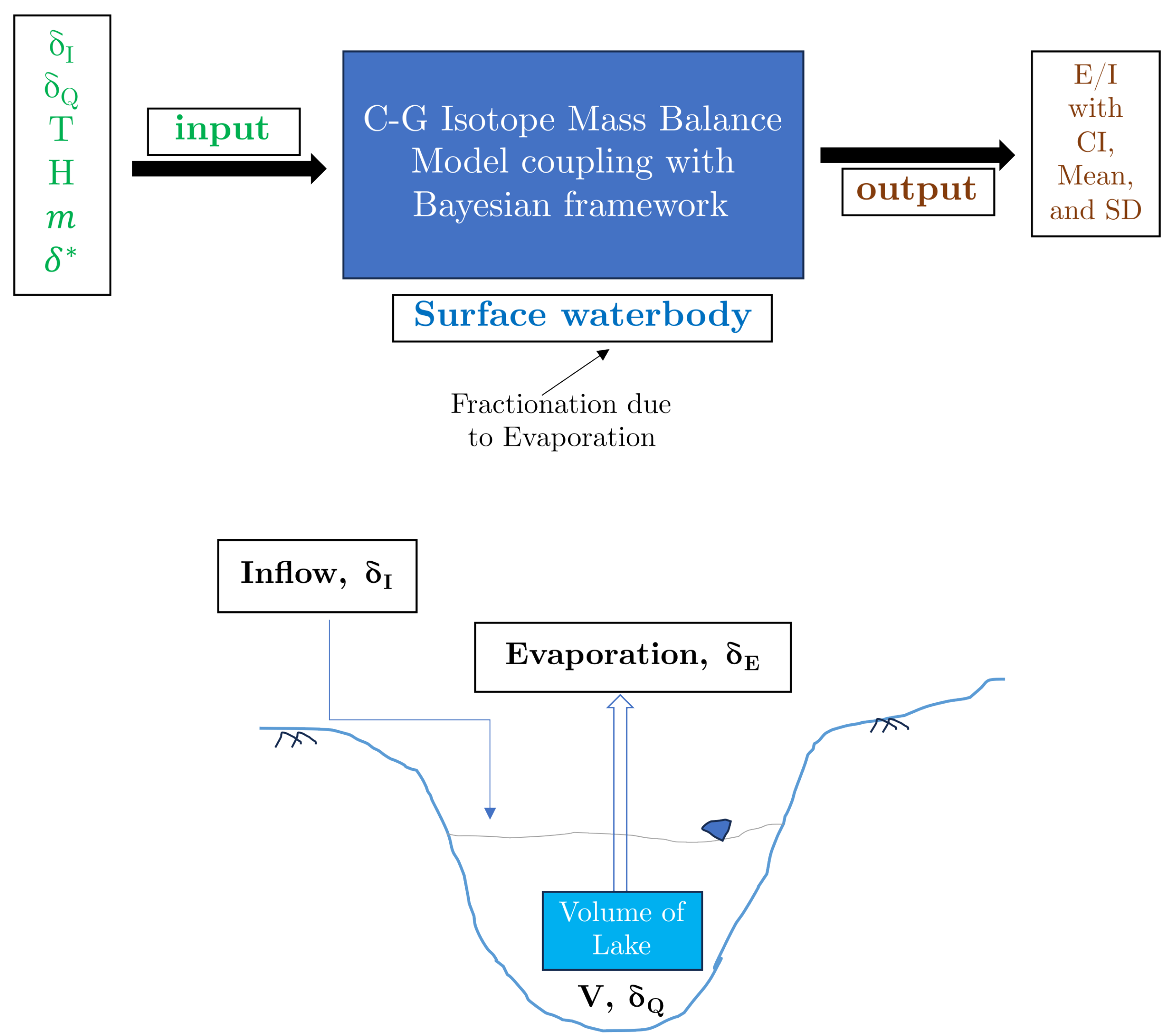
Figure 10.
Tracing water’s path in a tropical river from source to endpoint along a climate gradient.
Figure 10.
Tracing water’s path in a tropical river from source to endpoint along a climate gradient.
Author Contributions
Siva Naga Venkat Nara: Methodology, Investigation, Software, Formal analysis, Visualization, Writing- Original draft, Writing - Review & Editing. Prosenjit Ghosh: Conceptualization, Methodology, Investigation, Writing - Review & Editing, Resources, Supervision. Sekhar Muddu: Conceptualization, Methodology, Writing - Review & Editing, Funding acquisition, Resources, Supervision. R.D.Deshpande: Conceptualization, Methodology, Writing- Reviewing and Editing, Resources.
Conflicts of Interest
The authors declare no conflict of interest.
Appendix A
Appendix A.1
In our analysis, first focused on the trace plots which play an integral role in examining the convergence of our Markov Chain Monte Carlo (MCMC) chains. These plots, crucial to the understanding of the Bayesian analysis process, are constructed for each parameter in our model.
Figure A1.
Trace plots illustrating the Markov chain Monte Carlo (MCMC) sampling paths for the parameters: Intercept (), slope (), and standard deviation (). These plots provide a visual check for the convergence and mixing of the MCMC chains and help assess the posterior distributions of these parameters.
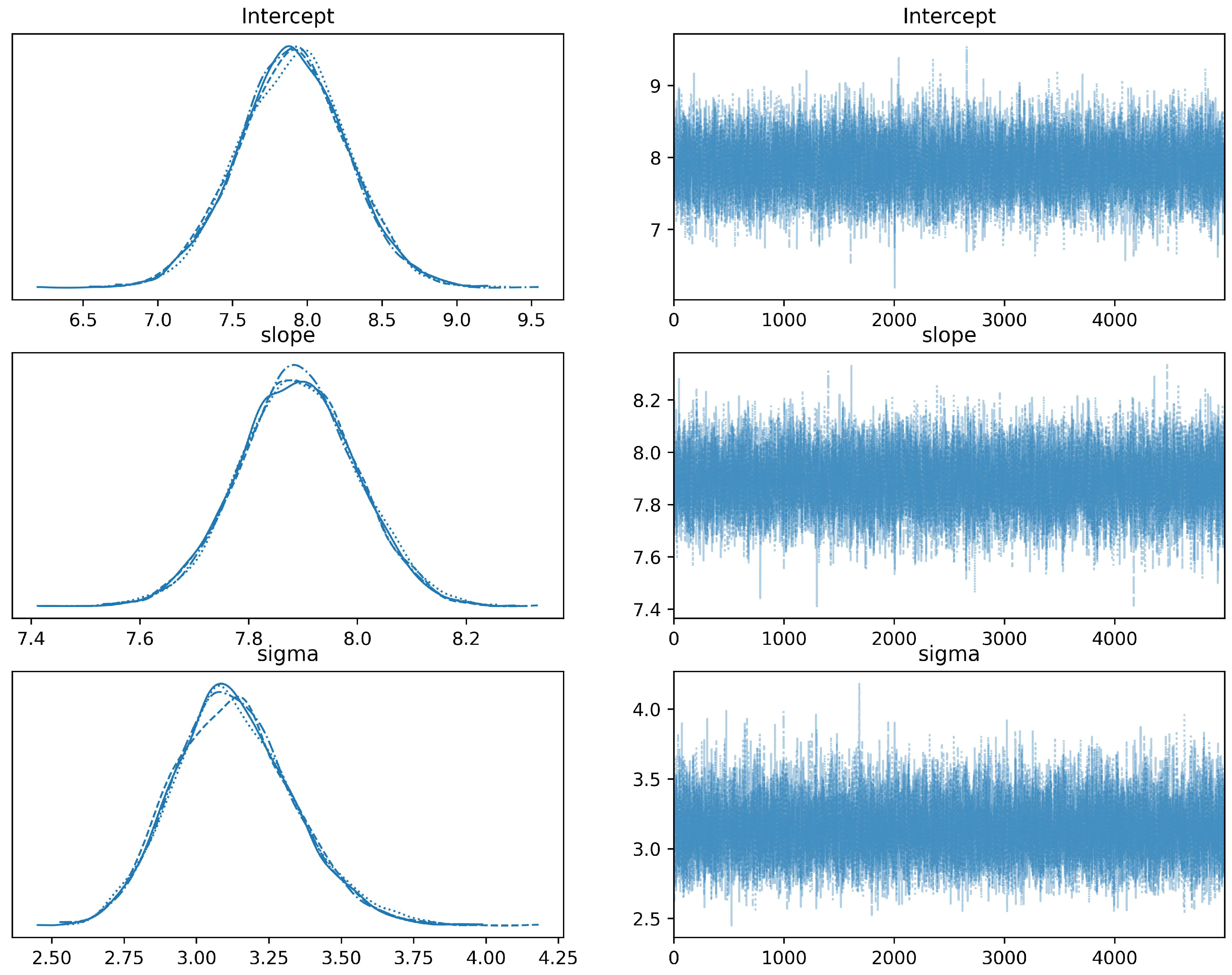
The trace plot consists of two sub-plots for each parameter. On the left, we present the kernel density estimates, a smoothed version of the histogram that gives us a clear depiction of the distribution of the sampled values. On the right, we display the sampled values traced over the iterations. The right-side plot enables us to visualize the ’random walk’ of the chain through the parameter space, a crucial aspect for diagnosing the mixing of the chains. A well-mixed and converged chain boosts our confidence in the robustness of our Bayesian linear regression model and the reliability of the resulting parameter estimates.
Figure A2.
Pair plot (scatter plot matrix) for the parameters: Intercept (), slope (), and standard deviation (). This plot provides a pairwise relationships overview between the different parameters, showing both scatter plots and kernel density estimations to visually assess the correlations and distributions.
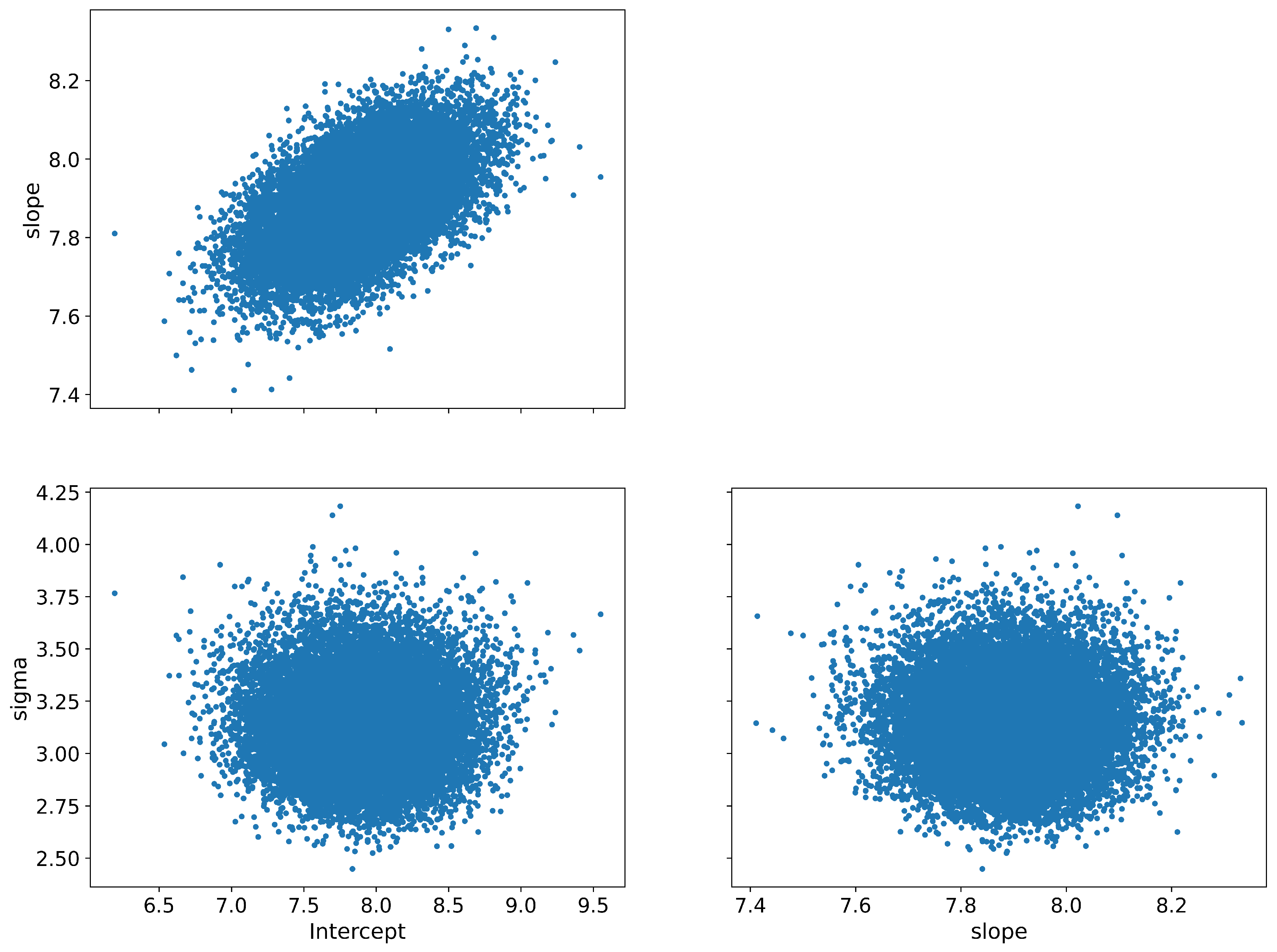
The pair plot, also known as a scatter plot matrix, is essential in our Bayesian analysis workflow, providing us with a visualization of the joint distributions between different model parameters. The pair plot’s primary utility lies in its ability to reveal patterns, correlations, and dependencies between the model’s parameters that might be hidden in the individual posterior distributions. For instance, in our model, we might be interested in understanding if and how the Intercept, slope, and sigma interact with each other.
References
- Brutsaert, W. Catchment-scale evaporation and the atmospheric boundary layer. Water Resources Research 1986, 22, 39S–45S. _eprint: https://onlinelibrary.wiley.com/doi/pdf/10.1029/WR022i09Sp0039S. [CrossRef]
- Diamond, R.E.; Jack, S. Evaporation and abstraction determined from stable isotopes during normal flow on the Gariep River, South Africa. Journal of Hydrology 2018, 559, 569–584. [CrossRef]
- Shen, Y.; Liu, C.; Liu, M.; Zeng, Y.; Tian, C. Change in pan evaporation over the past 50 years in the arid region of China. Hydrological Processes 2010, 24, 225–231. _eprint: https://onlinelibrary.wiley.com/doi/pdf/10.1002/hyp.7435. [CrossRef]
- Xiao, W.; Lee, X.; Hu, Y.; Liu, S.; Wang, W.; Wen, X.; Werner, M.; Xie, C. An Experimental Investigation of Kinetic Fractionation of Open-Water Evaporation Over a Large Lake. Journal of Geophysical Research: Atmospheres 2017, 122, 11,651–11,663. _eprint: https://onlinelibrary.wiley.com/doi/pdf/10.1002/2017JD026774. [CrossRef]
- Skrzypek, G.; Mydłowski, A.; Dogramaci, S.; Hedley, P.; Gibson, J.J.; Grierson, P.F. Estimation of evaporative loss based on the stable isotope composition of water using Hydrocalculator. Journal of Hydrology 2015, 523, 781–789. [CrossRef]
- Sun, Z.; Hu, C.; Wu, D.; Chen, G.; Lu, X.; Liu, X. Estimation of evaporation losses based on stable isotopes of stream water in a mountain watershed. Acta Geochimica 2021, 40, 176–183. [CrossRef]
- Gonfiantini, R. ENVIRONMENTAL ISOTOPES IN LAKE STUDIES. In The Terrestrial Environment, B; Elsevier, 1986; pp. 113–168. [CrossRef]
- Zhou, T.; Šimůnek, J.; Braud, I. Adapting HYDRUS-1D to simulate the transport of soil water isotopes with evaporation fractionation. Environmental Modelling & Software 2021, 143, 105118. [CrossRef]
- McGuire, K.; McDonnell, J. Stable Isotope Tracers in Watershed Hydrology. In Stable Isotopes in Ecology and Environmental Science; John Wiley & Sons, Ltd, 2007; pp. 334–374. Section: 11 _eprint: https://onlinelibrary.wiley.com/doi/pdf/10.1002/9780470691854.ch11. [CrossRef]
- Gibson, J.J.; Edwards, T.W.D. Regional water balance trends and evaporation-transpiration partitioning from a stable isotope survey of lakes in northern Canada. Global Biogeochemical Cycles 2002, 16, 10–1–10–14. _eprint: https://onlinelibrary.wiley.com/doi/pdf/10.1029/2001GB001839. [CrossRef]
- Gibson, J.J.; Reid, R. Water balance along a chain of tundra lakes: A 20-year isotopic perspective. Journal of Hydrology 2014, 519, 2148–2164. [CrossRef]
- Gunnell, Y.; Bourgeon, G. Soils and climatic geomorphology on the Karnataka plateau, peninsular India. CATENA 1997, 29, 239–262. [CrossRef]
- Sekhar, M.; Riotte, J.; Ruiz, L.; Jouquet, J.; Braun, J.J. Influences of Climate and Agriculture on Water and Biogeochemical Cycles: Kabini Critical Zone Observatory. Proceedings of the Indian National Science Academy 2016, 82. [CrossRef]
- Braun, J.J.; Descloitres, M.; Riotte, J.; Fleury, S.; Barbiéro, L.; Boeglin, J.L.; Violette, A.; Lacarce, E.; Ruiz, L.; Sekhar, M.; Mohan Kumar, M.; Subramanian, S.; Dupré, B. Regolith mass balance inferred from combined mineralogical, geochemical and geophysical studies: Mule Hole gneissic watershed, South India. Geochimica et Cosmochimica Acta 2009, 73, 935–961. [CrossRef]
- L. Collins, S.; Loveless, S.E.; Muddu, S.; Buvaneshwari, S.; Palamakumbura, R.N.; Krabbendam, M.; Lapworth, D.J.; Jackson, C.R.; Gooddy, D.C.; Nara, S.N.V.; Chattopadhyay, S.; MacDonald, A.M. Groundwater connectivity of a sheared gneiss aquifer in the Cauvery River basin, India. Hydrogeology Journal 2020, 28, 1371–1388. [CrossRef]
- Veena, M.; Achyuthan, H.; Eastoe, C.; Farooqui, A. A multi-proxy reconstruction of monsoon variability in the late Holocene, South India. Quaternary International 2014, 325, 63–73. [CrossRef]
- Michelsen, N.; van Geldern, R.; Roßmann, Y.; Bauer, I.; Schulz, S.; Barth, J.A.; Schüth, C. Comparison of precipitation collectors used in isotope hydrology. Chemical Geology 2018, 488, 171–179. [CrossRef]
- Buvaneshwari, S.; Riotte, J.; Sekhar, M.; Sharma, A.K.; Helliwell, R.; Kumar, M.S.M.; Braun, J.J.; Ruiz, L. Potash fertilizer promotes incipient salinization in groundwater irrigated semi-arid agriculture. Scientific Reports 2020, 10, 3691. Number: 1 Publisher: Nature Publishing Group. [CrossRef]
- Buttle, J.M.; McDonnell, J.J. Isotope tracers in catchment hydrology in the humid tropics. In Forests, Water and People in the Humid Tropics, 1 ed.; Bonell, M.; Bruijnzeel, L.A., Eds.; Cambridge University Press, 2005; pp. 770–789. [CrossRef]
- Epstein, S.; Mayeda, T. Variation of O18 content of waters from natural sources. Geochimica et Cosmochimica Acta 1953, 4, 213–224. [CrossRef]
- Rangarajan, R.; Ghosh, P. Role of water contamination within the GC column of a GasBench II peripheral on the reproducibility of 18O/16O ratios in water samples. Isotopes in Environmental and Health Studies 2011, 47, 498–511. [CrossRef]
- Rahul, P.; Ghosh, P.; Bhattacharya, S.K.; Yoshimura, K. Controlling factors of rainwater and water vapor isotopes at Bangalore, India: Constraints from observations in 2013 Indian monsoon: Rainwater and Water Vapor Isotopes. Journal of Geophysical Research: Atmospheres 2016, 121, 13,936–13,952. [CrossRef]
- Maurya, A.S.; Shah, M.; Deshpande, R.D.; Bhardwaj, R.M.; Prasad, A.; Gupta, S.K. Hydrograph separation and precipitation source identification using stable water isotopes and conductivity: River Ganga at Himalayan foothills. Hydrological Processes 2011, 25, 1521–1530. _eprint: https://onlinelibrary.wiley.com/doi/pdf/10.1002/hyp.7912. [CrossRef]
- Oza, H.; Padhya, V.; Ganguly, A.; Saikranthi, K.; Rao, T.N.; Deshpande, R.D. Hydrometeorological processes in semi-arid western India: insights from long term isotope record of daily precipitation. Climate Dynamics 2020, 54, 2745–2757. [CrossRef]
- Klaus, J.; McDonnell, J.J. Hydrograph separation using stable isotopes: Review and evaluation. Journal of Hydrology 2013, 505, 47–64. [CrossRef]
- Craig, H. Isotopic Variations in Meteoric Waters. Science 1961, 133, 1702–1703. Publisher: American Association for the Advancement of Science. [CrossRef]
- Bennett, K.; Gibson, J.; McEachern, P. Water-yield estimates for critical loadings assessment: Comparisons of gauging methods versus an isotopic approach. Canadian Journal of Fisheries and Aquatic Sciences 2008, 65, 83–99. [CrossRef]
- Gibson, J.J. Short-term evaporation and water budget comparisons in shallow Arctic lakes using non-steady isotope mass balance. Journal of Hydrology 2002, 264, 242–261. [CrossRef]
- Gibson, J.J.; Birks, S.J.; Jeffries, D.; Yi, Y. Regional trends in evaporation loss and water yield based on stable isotope mass balance of lakes: The Ontario Precambrian Shield surveys. Journal of Hydrology 2017, 544, 500–510. [CrossRef]
- Allison, G.B.; Leaney, F.W. Estimation of isotopic exchange parameters, using constant-feed pans. Journal of Hydrology 1982, 55, 151–161. [CrossRef]
- Gibson, J.; Edwards, T.; Bursey, G.; Prowse, T. Estimating Evaporation Using Stable Isotopes: Quantitative Results and Sensitivity Analysis for Two Catchments in Northern Canada. Hydrology Research 1993, 24, 79–94. [CrossRef]
- Craig, H.; Gordon, L. Deuterium and oxygen 18 variations in the ocean and the marine atmosphere. Stable Isotopes in Oceanographic Studies and Paleotemperatures. Spoleto, Italy 1965, pp. 9–130.
- Welhan, J.A.; Fritz, P. Evaporation pan isotopic behavior as an index of isotopic evaporation conditions. Geochimica et Cosmochimica Acta 1977, 41, 682–686. [CrossRef]
- Chen, Y.; Tian, L. Canal surface evaporation along the China’s South-to-North Water Diversion quantified by water isotopes. Science of The Total Environment 2021, 779, 146388. [CrossRef]
- Craig, H.; Gordon, L.I.; Horibe, Y. Isotopic exchange effects in the evaporation of water: 1. Low-temperature experimental results. Journal of Geophysical Research 1963, 68, 5079–5087. [CrossRef]
- Horita, J.; Rozanski, K.; Cohen, S. Isotope effects in the evaporation of water: a status report of the Craig–Gordon model. Isotopes in Environmental and Health Studies 2008, 44, 23–49. [CrossRef]
- Lewicki, M.P.; Lewicka-Szczebak, D.; Skrzypek, G. Supporting Information to: FRAME - Monte Carlo model for evaluation of the stable isotope mixing and fractionation 2022.
- Arellano, L.N.; Good, S.P.; Sánchez-Murillo, R.; Jarvis, W.T.; Noone, D.C.; Finkenbiner, C.E. Bayesian estimates of the mean recharge elevations of water sources in the Central America region using stable water isotopes. Journal of Hydrology: Regional Studies 2020, 32, 100739. [CrossRef]
- He, Z.; Unger-Shayesteh, K.; Vorogushyn, S.; Weise, S.M.; Duethmann, D.; Kalashnikova, O.; Gafurov, A.; Merz, B. Comparing Bayesian and traditional end-member mixing approaches for hydrograph separation in a glacierized basin. Hydrology and Earth System Sciences 2020, 24, 3289–3309. [CrossRef]
- Lewicka-Szczebak, D.; Jędrysek, M.O. Tracing and quantifying lake water and groundwater fluxes in the area under mining dewatering pressure using coupled O and H stable isotope approach. Isotopes in Environmental and Health Studies 2013, 49, 9–28. Publisher: Taylor & Francis _eprint: https://doi.org/10.1080/10256016.2012.700641. [CrossRef]
- Hoffman, M.D.; Gelman, A. The No-U-turn sampler: adaptively setting path lengths in Hamiltonian Monte Carlo. The Journal of Machine Learning Research 2014, 15, 1593–1623.
- Markovich, K.H.; Dahlke, H.E.; Arumí, J.L.; Maxwell, R.M.; Fogg, G.E. Bayesian hydrograph separation in a minimally gauged alpine volcanic watershed in central Chile. Journal of Hydrology 2019, 575, 1288–1300. [CrossRef]
- Salvatier, J.; Wiecki, T.V.; Fonnesbeck, C. Probabilistic programming in Python using PyMC3. PeerJ Computer Science 2016, 2, e55. [CrossRef]
- Rahul, P.; Ghosh, P.; Bhattacharya, S.K. Rainouts over the Arabian Sea and Western Ghats during moisture advection and recycling explain the isotopic composition of Bangalore summer rains: Isotopic Effect Due To Rainout. Journal of Geophysical Research: Atmospheres 2016, 121, 6148–6163. [CrossRef]
- Unnikrishnan Warrier, C.; Praveen Babu, M.; Sudheesh, M.; Deshpande, R.D. Studies on stable isotopic composition of daily rainfall from Kozhikode, Kerala, India. Isotopes in Environmental and Health Studies 2016, 52, 219–230. [CrossRef]
- Gonfiantini, R.; Wassenaar, L.I.; Araguas-Araguas, L.; Aggarwal, P.K. A unified Craig-Gordon isotope model of stable hydrogen and oxygen isotope fractionation during fresh or saltwater evaporation. Geochimica et Cosmochimica Acta 2018, 235, 224–236. [CrossRef]
- Horita, J.; Wesolowski, D.J. Liquid-vapor fractionation of oxygen and hydrogen isotopes of water from the freezing to the critical temperature. Geochimica et Cosmochimica Acta 1994, 58, 3425–3437. [CrossRef]
Figure 2.
Posterior distributions of the parameters: Intercept (), slope (), and standard deviation () with a 95% Highest Density Interval (HDI).
Figure 2.
Posterior distributions of the parameters: Intercept (), slope (), and standard deviation () with a 95% Highest Density Interval (HDI).
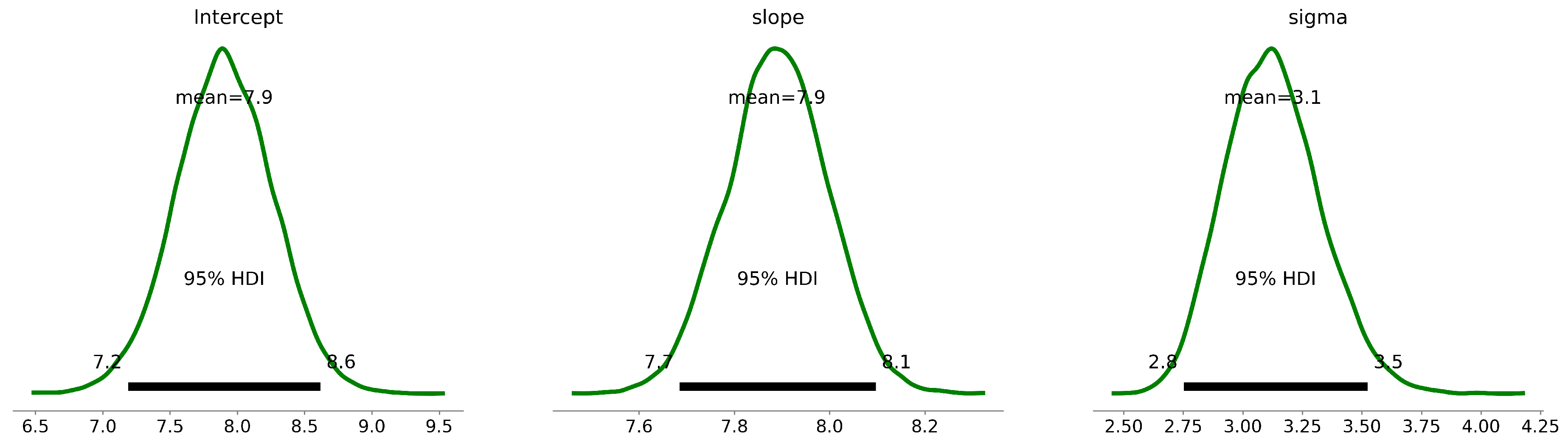
Figure 3.
Posterior distributions of the parameters: Intercept (), slope (), and standard deviation () with a 68% Highest Density Interval (HDI).
Figure 3.
Posterior distributions of the parameters: Intercept (), slope (), and standard deviation () with a 68% Highest Density Interval (HDI).
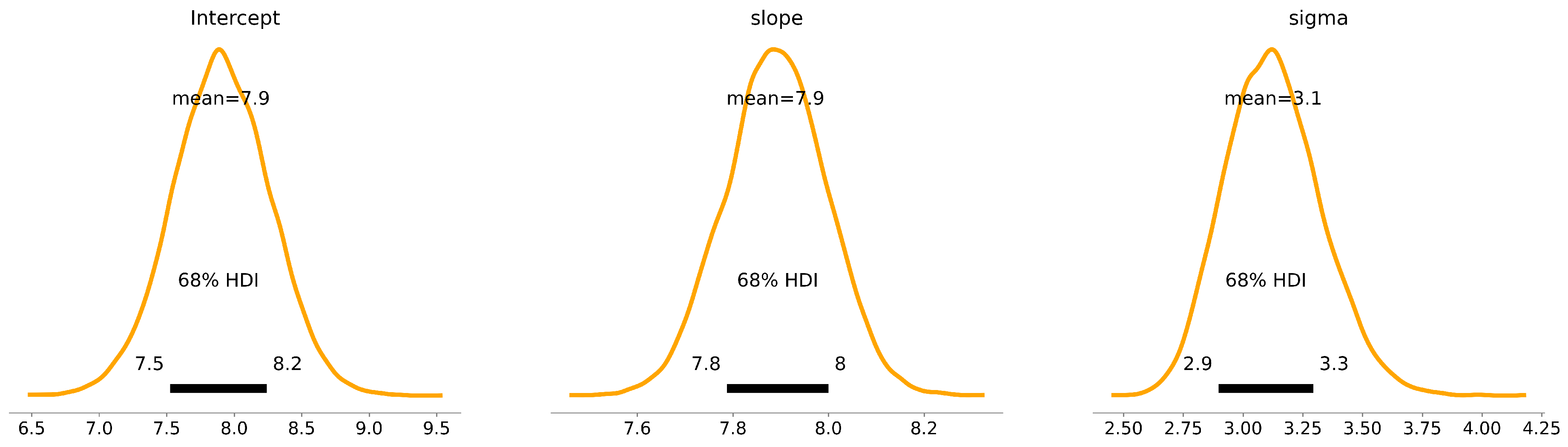
Figure 4.
Bayesian Linear Regression scatterplot of and Isotope Ratios in Meteoric Water with 68% Credible Intervals.
Figure 4.
Bayesian Linear Regression scatterplot of and Isotope Ratios in Meteoric Water with 68% Credible Intervals.
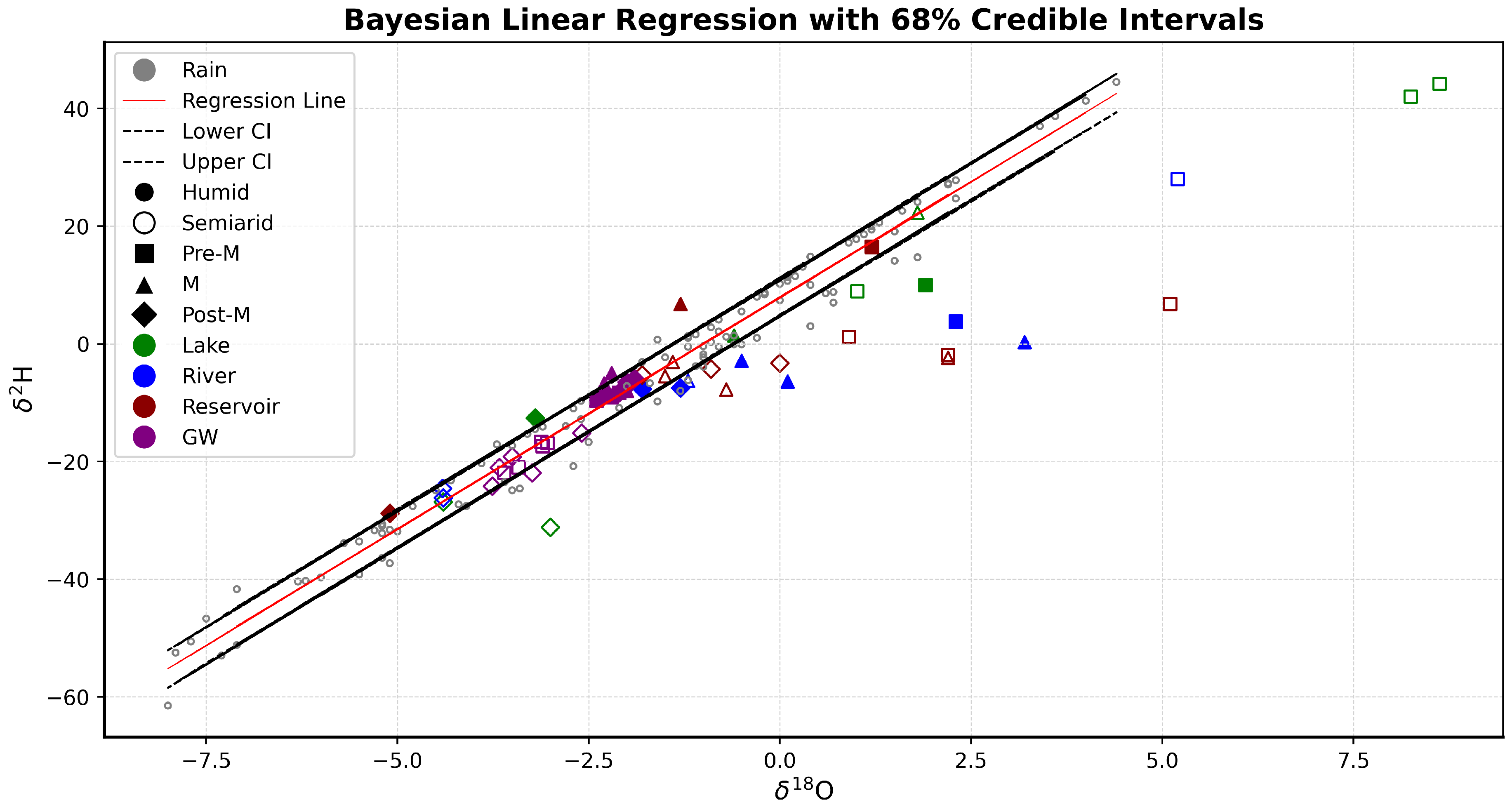
Figure 5.
Box Plots of Distribution and Variability of Groundwater Electrical Conductivity (EC) and Stable Water Isotopes ( and ) in Semiarid and Humid Climate Domains.
Figure 5.
Box Plots of Distribution and Variability of Groundwater Electrical Conductivity (EC) and Stable Water Isotopes ( and ) in Semiarid and Humid Climate Domains.
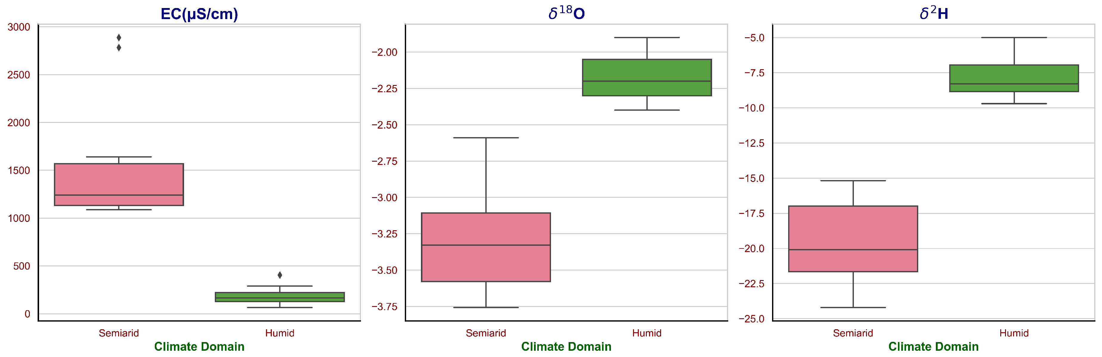
Figure 7.
Seasonal E/I Ratio Variation with Uncertainties - Bayesian Calibration for Lake Water
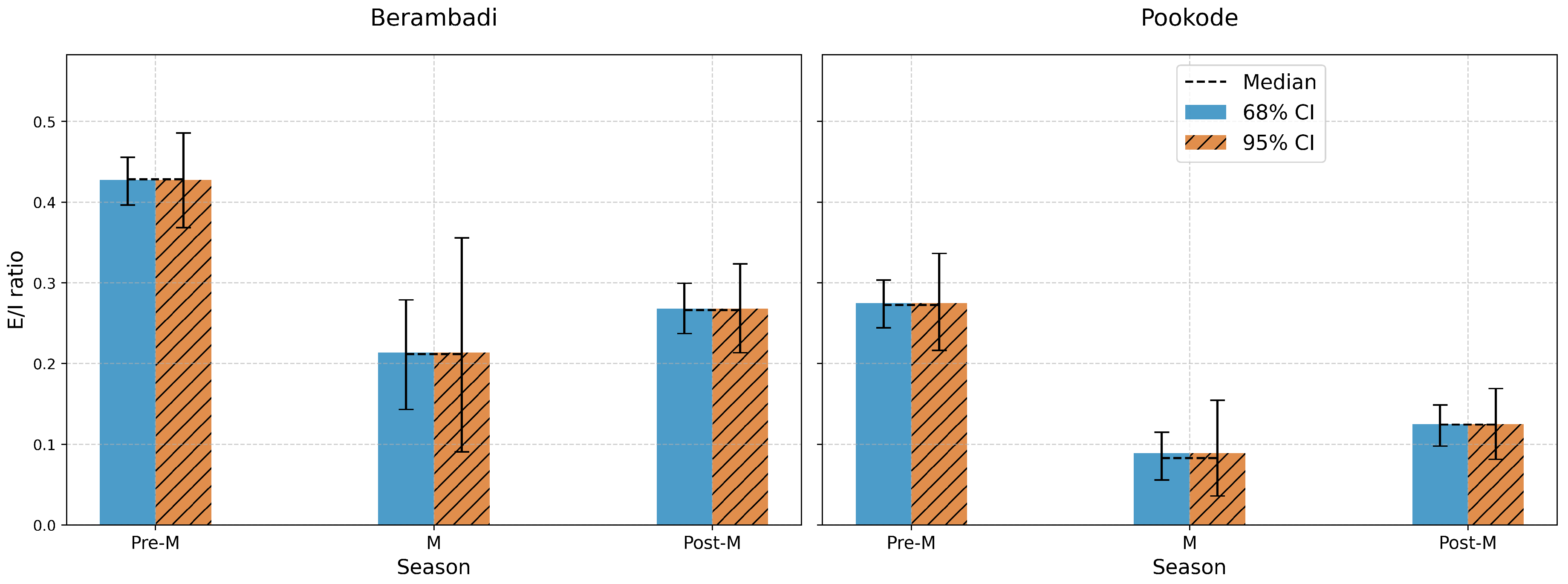
Figure 8.
Seasonal E/I Ratio Variation with Uncertainties - Bayesian Calibration for river segments.
Figure 8.
Seasonal E/I Ratio Variation with Uncertainties - Bayesian Calibration for river segments.
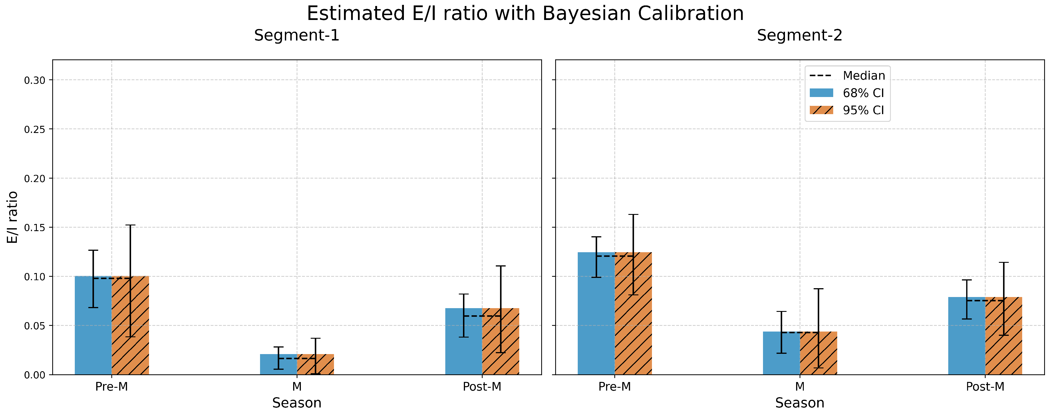
Table 1.
Overview of study locations in the Kabini Basin, detailing their type, geographical coordinates, elevation, climatic domain, and average annual rainfall.
Table 1.
Overview of study locations in the Kabini Basin, detailing their type, geographical coordinates, elevation, climatic domain, and average annual rainfall.
| S.no. | Type | Location | Lat | Long | Elevation | Climatic domain | Mean Annual Rainfall (mm) |
|---|---|---|---|---|---|---|---|
| 1 | Lake | Berambadi | 11.77 | 76.58 | 880 | Semi-arid | 800 |
| 2 | Pookode | 11.54 | 76.03 | 770 | Humid | 4000 | |
| 3 | River | Muthankera | 11.81 | 76.08 | 717 | Humid | 3000 |
| 4 | T. Narsipura | 12.23 | 76.89 | 660 | Semi-arid | 738 |
Table 4.
Seasonal Variation of Lake Isotope Composition and Other Hydrological Parameters in Semi-arid and Humid Regions
Table 4.
Seasonal Variation of Lake Isotope Composition and Other Hydrological Parameters in Semi-arid and Humid Regions
| Season | Location | pH | EC (S/cm) | T (°C) | h | d-excess | ||
|---|---|---|---|---|---|---|---|---|
| Pre-M | Berambadi | 8.3 | 567.1 | 31.8 | 0.53 | 42.0 | 8.2 | -23.93 |
| Pre-M | Berambadi | 8.8 | 530.2 | 31.8 | 0.53 | 44.2 | 8.6 | -24.78 |
| Pre-M | Berambadi | 7.6 | 184.5 | 31.8 | 0.53 | 8.9 | 1.0 | 0.84 |
| M | Berambadi | 6.6 | 159.0 | 24.2 | 0.79 | 4.4 | 1.8 | -10.0 |
| Post-M | Berambadi | 7.2 | 190.0 | 26.8 | 0.77 | -31.2 | -3.0 | -7.20 |
| Post-M | Berambadi | 7.3 | 195 | 26.9 | 0.71 | -26.9 | -4.4 | 8.30 |
| Pre-M | Pookode | 7.1 | 65.6 | 27.9 | 0.69 | 10.0 | 1.9 | -5.20 |
| M | Pookode | 6.4 | 50.6 | 21.9 | 0.92 | 1.4 | -0.6 | 6.20 |
| Post-M | Pookode | 7.2 | 65.3 | 22.9 | 0.85 | -12.6 | -3.2 | 13.0 |
Table 6.
Bayesian Framework Derived E/I for two lakes, using Craig-Gordon Model as Input. The Table Includes Mean, Median, Standard Deviation, and Confidence Intervals for Each Season.
Table 6.
Bayesian Framework Derived E/I for two lakes, using Craig-Gordon Model as Input. The Table Includes Mean, Median, Standard Deviation, and Confidence Intervals for Each Season.
| Season | Location | mean | median | stdev | CI68_low | CI68_up | CI95_low | CI95_up | ||
|---|---|---|---|---|---|---|---|---|---|---|
| Pre-M | Berambadi | 0.46 | 0.44 | 0.43 | 0.43 | 0.03 | 0.40 | 0.46 | 0.37 | 0.49 |
| M | Berambadi | 0.25 | 0.17 | 0.21 | 0.21 | 0.07 | 0.14 | 0.28 | 0.09 | 0.36 |
| Post-M | Berambadi | 0.39 | 0.25 | 0.27 | 0.27 | 0.06 | 0.24 | 0.30 | 0.21 | 0.33 |
| Pre-M | Pookode | 0.42 | 0.26 | 0.28 | 0.27 | 0.04 | 0.24 | 0.30 | 0.22 | 0.34 |
| M | Pookode | 0.15 | 0.07 | 0.09 | 0.08 | 0.06 | 0.06 | 0.12 | 0.04 | 0.15 |
| Post-M | Pookode | 0.19 | 0.11 | 0.12 | 0.12 | 0.03 | 0.10 | 0.15 | 0.08 | 0.17 |
Disclaimer/Publisher’s Note: The statements, opinions and data contained in all publications are solely those of the individual author(s) and contributor(s) and not of MDPI and/or the editor(s). MDPI and/or the editor(s) disclaim responsibility for any injury to people or property resulting from any ideas, methods, instructions or products referred to in the content. |
© 2023 by the authors. Licensee MDPI, Basel, Switzerland. This article is an open access article distributed under the terms and conditions of the Creative Commons Attribution (CC BY) license (http://creativecommons.org/licenses/by/4.0/).
Copyright: This open access article is published under a Creative Commons CC BY 4.0 license, which permit the free download, distribution, and reuse, provided that the author and preprint are cited in any reuse.


