
Submitted:
23 October 2023
Posted:
24 October 2023
You are already at the latest version
Abstract
Employing low tensor rank decompositions in image inpainting has attracted increasing attention. This paper exploits a novel tensor-augmentation schemes to transform an image (a low-order tensor) to a higher-order tensor without changing the total number of pixels. The developed augmentation schemes enhance the low-rankness of an image under three tensor decompositions: matrix SVD, tensor train (TT) decomposition, and tensor singular value decomposition (t-SVD). By exploiting the schemes, we solve the image inpainting problem with three low-rank con-strained models which use the matrix rank, TT rank, and tubal rank as constrained priors re-spectively. The tensor tubal rank and tensor train multi-rank are developed from t-SVD and TT decomposition respectively. We exploit efficient ADMM algorithms for solving the three models. Experimental results demonstrate that our methods are effective for image inpainting and supe-rior to numerous close methods.
Keywords:
image inpainting
; tensor decomposition
; rearrangement scheme
; unfolding matrix
; alternating direction multiplier method
1. Introduction
Image inpainting refers to the process of completing missing entries or restoring damaged regions of an image. It is a typical ill-posed inverse problem, generally solved by exploiting the image priors [1,2], such as smoothness, sparsity, and low rankness. In recent years, tensor analysis including tensor low-rank decomposition and tensor completion, has attracted increasing attention [3,4,5,6]. A color image itself is an order-3 tensor, or it can be used to construct a high order (greater than 3) tensor, then the image inpainting problem becomes a tensor completion problem. A tensor is more challenging to analyze than a matrix due to the complicated nature of higher-order arrays [7]. We can constrain the low tensor rank to recover the missing pixels. The effectiveness relies on the tensor rank. The lower the tensor rank is, the better the recovery results are. Thus, finding ways to decrease the tensor rank is essential in the tensor completion problem. Unlike matrix rank, the definition of tensor rank is not unique, and relates to the tensor decomposition scheme.
Low tensor-rank completion methods can be categorized according to the tensor decomposition frameworks they use [8]. The traditional tensor decomposition tools include CANDECOMP/PARAFAC (CP), and Tucker decomposition [8,9]. The recently proposed decomposition frameworks include tensor singular value decomposition (t-SVD) [10,11,12], tensor train (TT) decomposition [13,14], tensor tree (TTR) decomposition [6,15] etc. As we know, CP rank is hard to estimate. Tucker rank is multi-rank, whose elements are the ranks of mode-n matrices which are highly unbalanced. TT rank is also multi-rank, whose elements are the ranks of TT matrices. For a high-order tensor, the most TT matrices are more balanced than the mode-n matrices. Since the matrix rank minimization is only efficient when the matrix is balanced, TT decomposition is more suitable for describing global information of high-order tensors than Tucker decomposition. T-SVD defines the tubal rank of the high order tensor, which can be easily estimated according to a fast Fourier-based method. The tubal rank has been shown more efficient than the matrix-rank and Tucker multi-rank in video applications [16,17,18]. TTR rank is essentially equivalent to Tucker multi-rank.
Many popular tensor-completion methods have applied the traditional CP or Tucker decomposition on color image inpainting. Some recent works exploited the sparse Tucker core tensor and nonnegative Tucker factor matrices for image restoration [7,19,20]. Some works constrained the low rankness of the mode-n matrix caused by decomposition of a color image for inpainting [21,22]. Since low-tensor-rank constraint cannot fully capture the local smooth and global sparsity priors of tensors, some works combine Tucker and total variation (TV). The SPCTV (smooth PARAFAC tensor completion & total variation) method [23] used the PD (PARAFAC decomposition, a derivation of Tucker decomposition) framework, and constrained the TV (total variation) on every factor matrix of PD respectively. Some works combined the constraints of the low rankness of every mode-n matrix and the TV regularization on every mode-n matrix for color image inpainting [24,25]. Some works proposed data restoration methods based on Bayesian tensor completion [26,27,28,29].
The afore-mentioned methods all take the color image as an order-3 tensor directly and haven’t deeply explored the potential low-rank prior to a color image. Since TT decomposition is efficient for higher-order tensors, the TMac-TTKA method [30] first used the Ket augmentation (KA) scheme to permute the image to a high order data, then proposed the optimal models by enforcing low TT rankness. The KA scheme is proven to be efficient for improving the accuracy of color image/video inpainting and dynamic MR image reconstruction in TT rank based completion methods [30,31,32,33]. As far as we know, the KA scheme is the only one used to permute data into a high order data.
This paper aims to deeply explore the potential low-rank structure of the image and to find an efficient way to apply the SVD, t-SVD, and TT decomposition in the image inpainting problems. The contributions of our work are summarized as follows:
- First, we developed a novel rearrangement named as quarter augmentation (QA) scheme for permuting the image into three flexible forms of data. The first flexible QA scheme can permute an image into an unfolding matrix (with a low matrix rank structure). The second and the third flexible QA schemes can permute the color image into a balanced 3-order form of data (with low tubal rank structure) and a higher-order form of data (with low TT rank structure) respectively. Since those developed schemes are designed to exploit the internal structure similarity of the original data as much as possible, the rearranged data has the corresponding kind of low-rank structure.
- Second, based on the above QA scheme, we developed three image inpainting models that exploit the unfolding matrix rank, tensor tubal rank, and TT multi-rank of the rearranged data respectively for solving the image inpainting problem.
- Lastly, three efficient ADMM algorithms were developed for solving the above three models. Compared with numerous close image inpainting methods, the experimental results demonstrated the superior performance of our methods.
The remainder of this paper is organized as follows. In section II, we give the related work. In section III, we mainly introduce the proposed methods. Section IV the experimental results and analyses. The conclusion is given in section V.
2. Related work
In this section, we briefly introduce the KA scheme, the t-SVD decomposition, and tensor train decomposition. Notations and definitions are summarized in Table 1.
2.1. Ket Augmentation
The Ket Augmentation (KA) scheme was originally introduced by Latorre in [34] for casting a grayscale image into the real ket state of a Hilbert space. Bengua etc. [30] used KA to reshape a low-order tensor e.g. a color image to a higher-order tensor and proved that KA is efficient in improving the accuracy of the recovered image in TT-based completion.
2.2. T-SVD Decomposition
Definition 1
t-product [35]. For and , the t-product is a tensor of size where is given by . denotes the circular convolution between the two vectors, and , .
The t-SVD of is given by
where and are orthogonal tensors of size and respectively. is a rectangular f-diagonal tensor of size and * denote t-product [35], denotes tensor transpose defined in [35].
Figure 2 depicts the t-SVD of an order-3 tensor [4,36]. Tensor rank defined in t-SVD is tensor tubal rank, which is the number of nonzero singular tubes in . [36] proposed the fast Fourier-based method to calculate the tubal rank, and used tensor nuclear norm (TNN) as the convex relaxation of the tensor tubal rank.
where is the tensor obtained by applying the 1D FFT along the third dimension of , denotes nuclear norm, and
2.3. Tensor Train Decomposition
Given a tensor , tensor train (TT) decomposition [13,14] can decompose it to order-3 tensors , . The tensor rank defined in TT decomposition is a multi-rank i.e. , which is combined with the second-dimensional size of each . The details of TT decomposition are shown in the following formula and Figure 3 [31,32,33].
The widely used way to find TT rank is to estimate the rank of each TT matrix [37] as the element of . The TT matrix () with rank is the mode- matricization of the tensor with the size of , where , .
3. Methods
3.1. Quarter Augmentation
To deeply explore the more efficient low-rank structure of an image, we develop a novel rearrangement scheme named as quarter augmentation (QA) scheme to turn a color image into other forms of data. The QA schemes can maintain the internal similarity of the original image in the rearranged data.
The basic QA scheme: For example, as shown in Figure 4 (a), M is a 2D matrix (). We first extract the entries of M every other row and column to get four smaller matrices. Each smaller matrix with a size of . Then we place these four smaller matrices along the third dimension in a designed order. Lastly, a 3D tensor of size is obtained from the matrix M without changing the total number of entries. The entries in the four smaller matrices are labeled as the MATLAB notation , , and respectively. If M is smooth (most images satisfy), the four smaller matrices are similar in structure due to the adjacent entries.
Applying the basic QA scheme on the single Lena image, the Lena image can be divided into 4 smaller Lena images, and as shown in Figure 4 (b) the four smaller Lena images are similar to each other. In Figure 4 (c), the pixel values curves of the four smaller images have overlapped into one curve. We can say that the similarity of local image structure is mainly maintained by the basic QA scheme.
Under this basic QA scheme, three flexible QA schemes are proposed for permuting the image into three flexible forms of data. The three flexible QA schemes can enhance the low-rankness for an image by matrix SVD, tensor train decomposition, and tensor-SVD respectively. Then, by exploiting the flexible QA schemes, three low-rank constrained methods which use the TT rank, tubal rank, and matrix rank as constrained priors respectively are exploited for image inpainting.
The three flexible QA schemes and methods are described in detail in the following three sections.
3.2. Method 1: The Low Unfolding Matrix Rank-Based Method
The unfolding method is widely used to permute the order-3 video or dynamic magnetic resonance images into an unfolding matrix, and then exploit the low rankness of this matrix for data reconstruction [21,38]. The unfolding matrix has a low-rank structure because of the similarity of every slightly changed slice along the time dimension.
We try to dig out the potential low unfolding-matrix rankness of a color image by a flexible QA scheme, and we call this scheme the first flexible QA scheme.
Take a 256×256×3 Lena image as an example, as shown in Figure 5 (a), we first permute the image into the 3-order tensor size of 32×32×192 by the basic QA scheme, then unfold the similar slices of this 3-order. Lastly, the balanced1 unfolding matrix size of 1024×192 is obtained. Since the slices (32×32) in the 3-order tensor are similar, the unfolding matrix is low rank, as shown in Figure 5 (b). In practice, the size of the designed unfolding matrix should be balanced such that the minimization of the unfolding matrix rank is efficient.
We exploit the low unfolding matrix rank in image inpainting and give the low unfolding matrix-rank-based model as follows.
where denotes the image to be recovered, denotes the operator of permuting the image into a suitable 3-order tensor by multiple basic QA schemes. denotes the operator of the unfolding process, which unfolding every slice along the third dimension of the 3-order tensor . is the position without painting, is the painted image with damaged entries at the positions .
To reduce the computational complexity, in the model (1), the following SVD-free approach [39,40] is exploited to constrain the low rankness of the unfolding matrix instead of the nuclear norm.
Besides, since total variation (TV) has been proved as an effective constraint of smooth prior [41,42], incorporate model (1) with 2D TV to exploit the local smooth priors of visual image data. Then, the image inpainting model (1) turns to the following.
where is the regularization parameter.
We conduct the algorithm by alternating direction method of multipliers (ADMM) for solving the low unfolding matrix rank and TV-based image inpainting model (3). Firstly, introduce an auxiliary variable , where is the finite difference operator, and then rewrite (3) as the unconstrained convex optimization problem (4).
where denotes the indicator function:
,
and are the Lagrangian multipliers for variables and respectively. The regularization parameter is used to balance the low rankness and sparsity constraints (i.e. TV), the penalty parameters and generally affect the convergence of the algorithm. By applying ADMM, each sub-problem is performed at each iteration t as follows:
The initial and can be determined by solving the following optimization problem using the LMaFit method [43].
The whole algorithm for solving the model (3) is shown in Table 2.
3.3. Method 2: The Low Tubal-Rank-Based Method
Tensor-SVD decomposition has been efficiently used in the video image completion and dynamic MR image reconstruction problem [16,44,45,46]. Since the color image is highly unbalanced in the size of three dimensions, which is not suitable for the low tubal rank constraint, we exploit the second flexible QA scheme to deeply dig out the potential low tubal-rank prior information.
Considering that tubal rank minimizations are more efficient for the balanced tensor [10], we first turn the unbalanced image into the balanced order-3 data by the second flexible QA scheme.
Take the color image size of 256×256×3 as an example, as shown in Figure 6 (a), we can obtain the order-4 tensor size of 128×128×4×3 by the basic QA schemes, and then multiplying the basic QA schemes we can obtain the order-4 tensor size of 64×64×4×4×3. Lastly, we reshape the order-4 tensor into the balanced order-3 tensor size of 64×64×48. Here, the context of ‘balanced’ is that the size changes from the unbalanced 256×256×3 to the more balanced size of 64×64×48. In practice, the size of the designed order-3 tensor should be as balanced as possible. We call the above the second flexible QA scheme.
In Figure 6 (b), we show the low tubal rankness of the balanced order-3 data (with the size of here) by plotting which is defined as follows.
Then, TNN is used to enforce the tensor tubal rank in the image inpainting model as follows.
where denotes the operator of permuting the color image into a more ‘balanced’ order-3 tensor by the second flexible QA scheme. Combining the low tubal rank and sparsity, we introduce auxiliary variables , and , then rewrite (12) as the following unconstrained convex optimization problem.
where is the third size of the 3-order tensor . We conduct the algorithm by ADMM for solving model (13) as shown in Table 3.
3.4. Method 3: The Low TT-Rank-Based Method
TT decomposition works better on higher-order tensors than Tucker decomposition. To fulfill TT decomposition efficiently, we first exploit the third flexible QA scheme to permute the 3-order image into a higher-order tensor. Based on the basic QA scheme, high-order tensors can be obtained flexibly.
The third flexible QA scheme is shown below. We take a matrix as an example, as shown in Figure 7 (a). We first turn a 2-order matrix into a 3D tensor via the basic QA scheme and then repeat the basic QA to obtain the final 4D tensor with the size of . The entry comes from the ith smaller matrix of the first basic QA scheme, and the jth smaller matrix of the second basic QA scheme is labeled as the MATLAB notation . By analogy, the third flexible QA scheme can permute a matrix with the size of to order- tensor with the size of . An RGB image with the size of can be permuted into an order- tensor with the size of . The third flexible QA scheme should ensure that the designed tensor has a higher order.
We permute the Lena image into a high-order tensor via the third flexible QA scheme, and then obtain the TT matrices of the augmented tensor. We name those TT matrices as QA-TT matrices, and their singular values are shown in Figure 7 (b), which demonstrates the low TT rankness of the rearranged tensor.
Then, we enforce the low TT rankness to improve the inpainting accuracy. The third model is as follows.
where stands for the third flexible QA used to permute image into a high-dimensional tensor. We name the tensor obtained by the third flexible QA scheme as a QA tensor. is the operator that converts a tensor into the nth TT matrix, . The order of QA tensor is . The inverse operators corresponding to and are and respectively. The weight is given by:
where is the size of the QA tensor.
Combining the low TT rank and sparsity constraints, we introduce auxiliary variables and , rewrite (14) as the following unconstrained convex optimization problem, for all .
By applying ADMM, each sub-problem is performed at each iteration t. Lastly, we obtain by , where represents the optimal solution of the nth subproblem. The whole algorithm for solving the model (16) is shown in Table 4.
4. Experimental Results and Analyses
In this section, we conduct the above methods 1-3 for solving image inpainting problems. For simplicity, we denote methods 1-3 which only exploit low unfolding matrix rank, low tensor tubal rank, and low tensor train rankness as UfoldingLR, TTLR, and tSVDLR methods respectively. The methods that enhance the low rank and total variation constraints simultaneously are denoted as UnfoldingLRTV, tSVDLRTV, and TTLRTV methods respectively. We denote the low matrix-rank completion method which is solved by the model (17) and ADMM algorithm as the MatrixLR method.
We denote the method that only exploits sparsity in the gradient domain and is solved by the ADMM algorithm as the TV method. Besides, we conduct the following numerous close methods for comparison, some of their codes are available online.
STDC: the method exploited the images into three factor matrices and one core tensor for image inpainting [7,19,20]2.
HaLRTC: the method constrained the low rankness of the three mode-n matrices caused by decomposition of a color image for inpainting and which was solved by the ADMM [21,22]3.
SPCTV4: the smooth PARAFAC tensor completion and total variation method [23], which used the PD (PARAFAC decomposition, a derivation of Tucker decomposition) framework and constrained the TV on every factor matrix of PD respectively.
LRTV: the methods combined the constraints of the low rankness of every mode-n matrix and the TV regularization on every mode-n matrix for color image inpainting [24,25]5.
All simulations were carried out on Windows 10 and MATLAB R2019a running on a PC with an Intel Core i7 CPU 2.8GHz and 16GB of memory. For a fair comparison, every method is conducted with its optimal parameters to ensure every method has the best performance. The reconstruction quality is quantified using the peak signal-to-noise ratio (PSNR) and structural similarity (SSIM)7 [37]. The original color images (from the standard image database) and missing patterns used in the experiments are shown in Figure 8.
We set the maximum number of iterations and convergence condition in all our methods (UnfoldingLRTV, tSVDLRTV, and TTLRTV). The pixel range of all the images is normalized to 0-1. In UnfoldingLR, tSVDLR, and TTLR methods, we set 0.04, 0.002, and 0.6 respectively. In UnfoldingLRTV, Tsvdlrtv, and TTLRTV methods, we set the parameter set as (0.4, 0.004, 2), (0.6, 0.07, 0.1), and (0.7, 0.03, 0.1) respectively.
4.1. Analyses of the Three Flexible QA Schemes
Next, we call the first, second, and third flexible QA schemes QA scheme briefly. The PSNRs (dB)/SSIMs of the UnfoldingLR, tSVDLR, and TTLR methods with and without the QA scheme are shown in Table 5. The red numerical values correspond to the worst results. We can see that, without the QA scheme, Lena and Airplane cannot be recovered. The UnfoldingLR, tSVDLR, and TTLR methods with the QA scheme have better numerical results than those without the QA scheme. In the low matrix-rank completion method (i.e. MatrixLR), no QA scheme is applied, i.e. the color image is dealt with as three-channel matrices directly.
Due to the support of the QA scheme, the low tensor-rank based methods (TTLR, tSVDLR, and UnfoldingLR) with the QA scheme provide better results than the traditional low matrix-rank completion method (i.e. MatrixLR method). So, the QA scheme is successful to be used as the first step to deeply explore the low tensor rank prior to an image.
The KA scheme and the third flexible QA scheme both can rearrange an image into a high-order tensor. However, our QA scheme is different from the KA scheme used in [21]. The KA scheme maintains the local block similarity of the image, while the third flexible QA scheme uses adjacent pixels to maintain the global similarity of the image. We conduct the comparison of KA and the third flexible QA scheme under the corresponding TMac-TTKA [21] and TTLR methods. As shown in Figure 9, the small blocks are obvious in the recovered images by the TMac-TTKA method. The images recovered by the TTLR method preserve more details and without the obvious blocks.
4.2. Analyses of the Methods Exploiting Both Low Rankness and Sparsity
In this section, we analyze the recovery results of the methods both exploiting low rankness and sparsity. Figure 10, Figure 11 and Figure 12 show the visual comparisons of the eleven methods for recovering the House, Lena, and Baboon images respectively. Table 6 shows the PSNR (dB)/SSIM results of the nine methods for recovering different color images under different missing patterns. Figure 13 depicts the PSNR curves of the inpainting results of the different methods, the missing ratio ranges from 10% to 70% under a random missing pattern.
As shown in Figure 10, Figure 11, Figure 12 and Figure 13 and Table 6, compared to the numerous close STDC, HaLRTC, FBCP, TMac-TTKA, SPCTV, and LRTV methods, the UnfoldingLRTV, tSVDLRTV, and TTLRTV methods have the super performance on both visual and quantity results. The SPCTV and LRTV methods also enhance the low rankness and sparsity simultaneously, but the results are worse than our methods.
Table 7 shows the PSNR (dB)/SSIM results of the eight methods: MatrixLR method only constrains the low matrix rank; TV method only exploits the TV prior; The UnfoldingLR, tSVDLR, and TTLR methods only constrain the low unfolding matrix rank, low tubal rank and low TT rank respectively; The UnfoldingLRTV, tSVDLRTV, and TTLRTV methods combine both sparsity and low tensor rankness. As shown in Table 7, the combination of sparsity and low tensor rankness constraints can yield better inpainting results than enforcing sparsity or low rankness alone. TTLR method is more efficient than the MatrixLR, and TV methods. The results of the tSVDLR method and TTLR method are comparable. The UnfoldingLR method provides the best results among the TTLR, tSVDLR, TuckerLR, MatrixLR, and TV methods. UnfoldingLRTV, tSVDLRTV, and TTLRTV methods have improved numerical results than the corresponding UnfoldingLR, tSVDLR, and TTLR methods, which demonstrates that TV prior is efficient in improving the accuracy of low-rank based inpainting methods.
The visual and numerical PSNR (dB)/SSIM comparisons of our methods for recovering the pepper image under 80% random missing patterns are shown in Figure 14. In the first row of Figure 14, the methods only exploit low-rank constraints. As shown in the color box, there are small blocky errors in the recovered image, these are caused by the QA scheme. This phenomenon can be solved by combining the constraints of low rank and sparsity (TV), as shown in the second row of Figure 14.
All in all, due to the support of the QA scheme and the efficient TV prior, the low tensor-rank based methods (UnfoldingLRTV, tSVDLRTV, and TTLRTV) are superior to other close low tensor-rank based methods. The UnfoldingLRTV method provides the best results among all the methods conducted in this paper.
4.3. Analyses of TTLR and TTLRTV Methods
In this section, we mainly focus on the analyses of the TT based methods (i.e. TTLR and TTLRTV) in detail. Since TT rank is multi-rank, how does every TT matrix rank affect the final result? We answer this question with the below experimental results.
We conducted the experiments on recovering House, Lena, and Airplane images with a size of 256×256×3. The random missing patterns have four missing ratios: 10%, 30%, 50%, and 70% respectively. We label the 8 TT matrices as k=1, 2, …, 8. Then the PSNR (dB) results of (the optimal solution of the nth subproblem which exploits the nth TT matrix rank) in TTLR and TTLRTV methods are shown in Figure 15.
From Figure 15, we can see that, the PSNR (dB) results of each subproblem is steeply different in the TTLR method, which demonstrates that each TT matrix rank contributes different PSNR result. Since there are no rules to find which TT matrix rank meets the best PSNR result, we should combine each solution of to obtain the final , i.e. . Comparing the PSNR curves of TTLR and TTLRTV method in Figure 15, the PSNR (dB) results of each subproblem is slightly different in the TTLRTV method which demonstrates that the combination of TT and TV can make the PSNR more balanced among all k.
4.4. Runtime and Complexity Analysis
From a high-dimensional curse perspective, converting an image to a higher-order tensor can result in increased complexity, which inevitably leads to a longer runtime. We compare our methods (UnfoldingLRTV, tSVDLRTV, and TTLRTV) with the traditional MatrixLR method and the close STDC, HaLRTC, FBCP, SPCQV, and LRTV methods in running time, as shown in Table 8.
UnfoldingLRTV methods: In the first step, the QA scheme is used to decompose a single image into several small graphs. Because of the similarity of these small graphs, the QA tensor can be reduced to a matrix with a low-rank structure in an unfolding way. Ignoring TV constraints, the unfoldingLRTV method only needs to solve the low-rank matrix completion problem of an unfolding matrix, so the running time is similar to the traditional MatrixLR method, and the accuracy is higher than the traditional MatrixLR method.
The tSVDLRTV methods: Since the color image is highly unbalanced in the size of three dimensions, which is not suitable for the low tubal rank constraint, we use the QA scheme to rearrange an image into a third-order tensor with a more balanced size of every dimension. Then we use TNN to constrain the low tubal rank of the rearranged tensor, due to the fast Fourier scheme, it is necessary to perform a low-rank matrix constraint on each frontal slice after the third-dimensional Fourier transform. At this time, the SVD decomposition process will increase the time consumption.
TTLRTV methods: TT multi-rank is the combination of the rank of each TT matrix. The TTLRTV method essentially completes the same data amount N-1 times, where N is the order of the QA tensor. So, although the TITRTV method is effective, it is necessarily more computationally expensive than the low matrix-rank completion method.
In summary, among the three methods, the UnfoldingLRTV method achieves the best performance both in accuracy and runtime; The TTLRTV method reaches better accuracy, but it is time-consuming; The tSVDLRTV method has moderate performance both in runtime.
All in all, the above three methods can deeply exploit the potential low-rank prior of an image and have been successfully used for image inpainting problems, which demonstrates that the three flexible QA schemes are perfect ways to explore the low-rank prior of an image.
5. Conclusions
To effectively explore the potential of low tensor rank prior to an image, we first exploited a rearrangement scheme (QA) for permuting the color image (3-order) into three flexible rearrangement forms (with more efficient low tensor rank structure). Based on the scheme, three optimization models by exploiting the low unfolding matrix rank, low tensor tubal rank, and low TT multi-rank were proposed to improve the accuracy in image inpainting. Combined with TV constraints, we developed efficient ADMM algorithms for solving those three optimization models. The experimental results demonstrate that our low tensor-rank-based methods are effective for image inpainting, and are superior to the low matrix-rank completion method and numerous close methods. The low tensor rank constraint is effective for image inpainting, which is mainly due to the support of the QA scheme.
Author Contributions
Conceptualization, S.M.; methodology, S.M.; investigation, S.M. and Y.F.; resources, S.M. and S.F.; writing—original draft preparation, S.M. and S.F.; writing—review and editing, S.F., W.Y. and Y.F.; supervision, L.L. and W.Y.; funding acquisition, S.M. and L.L. All authors have read and agreed to the published version of the manuscript.
Funding
This work was funded by the National Key Laboratory of Science and Technology on Space Microwave, No. HTKJ2021KL504012; Supported by the Science and Technology Innovation Cultivation Fund of Space Engineering University, No. KJCX-2021-17; Supported by the Information Security Laboratory of National Defense Research and Experiment, No.2020XXAQ02.
Institutional Review Board Statement
Not applicable.
Informed Consent Statement
Not applicable.
Data Availability Statement
Not applicable.
Conflicts of Interest
The authors declare no conflict of interest.
References
- Pendu, M.; Jiang, X.; Guillemot, C. Light field inpainting propagation via low rank matrix completion. IEEE Trans. Image Process. 2018, 27, 1989–1993. [Google Scholar] [CrossRef] [PubMed]
- Yu, Y.; Peng, J.; Yue, S. A new nonconvex approach to low-rank matrix completion with application to image inpainting, Multidim. Syst. Signal Process. 2018, 30, 145–174. [Google Scholar]
- Gong, X.; Chen, W.; Chen, J. A low-rank tensor dictionary learning method for hyperspectral image denoising. IEEE Trans. Signal Process. 2020, 68, 1168–1180. [Google Scholar] [CrossRef]
- Su, X.; Ge, H.; Liu, Z.; Shen, Y. Low-Rank tensor completion based on nonconvex regularization. Signal Process. 2023, 212, 109157. [Google Scholar] [CrossRef]
- Ma, S.; Ai, J.; Du, H.; Fang, L.; Mei, W. Recovering low-rank tensor from limited coefficients in any ortho-normal basis using tensor-singular value decomposition. IET Signal Process. 2021, 19, 162–181. [Google Scholar] [CrossRef]
- Liu, Y.; Long, Z.; Zhu, C. Image completion using low tensor tree rank and total variation minimization. IEEE Trans. Multimedia. 2018, 21, 338–350. [Google Scholar] [CrossRef]
- Gong, W.; Huang, Z.; Yang, L. Accurate regularized Tucker decomposition for image restoration. Appl. Math. Model. 2023, 123, 75–86. [Google Scholar] [CrossRef]
- Long, Z.; Liu, Y.; Chen, L. Low rank tensor completion for multiway visual data. Signal Process. 2019, 155, 301–316. [Google Scholar] [CrossRef]
- Kolda, T.; Bader, B. Tensor decompositions and applications. SIAM Rev. 2009, 51, 455–500. [Google Scholar] [CrossRef]
- Kilmer, M.; Braman, K.; Hao, N. Third-order tensors as operators on matrices: a theoretical and computational framework with applications in imaging. SIAM J. Matrix Anal. Appl. 2013, 34, 148–172. [Google Scholar] [CrossRef]
- Semerci, O.; Hao, N.; Kilmer, M. Tensor-based formulation and nuclear norm regularization for multienergy computed tomography. IEEE Trans. Image Process. 2014, 23, 1678–1693. [Google Scholar] [CrossRef] [PubMed]
- Zhou, P.; Lu, C.; Lin, Z.; Zhang, C. Tensor factorization for low-rank tensor completion. IEEE Trans. Image Process. 2018, 3, 1152–1163. [Google Scholar] [CrossRef] [PubMed]
- Oseledets, I.; Tyrtyshnikov, E. TT-cross approximation for multidimensional arrays. Linear Algebra Appl. 2010, 432, 70–88. [Google Scholar] [CrossRef]
- Oseledets, I. Tensor-train decomposition. Siam J.Sci. Comput. 2011, 33, 2295–2317. [Google Scholar] [CrossRef]
- Hackbusch, W.; Kuhn, S. A new scheme for the tensor representation. J. Fourier Anal. Appl. 2009, 15, 706–722. [Google Scholar] [CrossRef]
- Zhang, Z.; Aeron, S. Exact tensor completion using T-SVD. IEEE Trans. Signal Process. 2017, 65, 1511–1526. [Google Scholar] [CrossRef]
- Lu, C.; Feng, J.; Chen, Y.; Liu, W.; Lin, Z.; Yan, S. Tensor robust principal component analysis with a new tensor nuclear norm. IEEE Trans. Pattern Anal. Mach. Intell. 2020, 42, 925–938. [Google Scholar] [CrossRef] [PubMed]
- Du, S.; Xiao, Q.; Shi, Y.; Cucchiara, R.; Ma, Y. Unifying tensor factorization and tensor nuclear norm approaches for low-rank tensor completion. Neurocomput. 2021, 458, 204–218. [Google Scholar] [CrossRef]
- Chen, Y.; Hsu, C.; Liao, H. Simultaneous tensor decomposition and completion using factor priors. IEEE Trans. Pattern Anal. Mach. Intell. 2014, 36, 577–591. [Google Scholar] [CrossRef]
- Xue, J.; Zhao, Y.; Liao, W. ; Enhanced sparsity prior model for low-rank tensor completion. IEEE Trans. Neural. Netw. Learn. Syst. 2019, 31, 4567–4581. [Google Scholar] [CrossRef]
- Liu, J.; Musialski, P.; Wonka, P. Tensor completion for estimating missing values in visual data. IEEE Trans. Pattern Anal. Mach. Intell. 2013, 35, 208–220. [Google Scholar] [CrossRef] [PubMed]
- Qin, M.; Li, Z.; Chen, S.; Guan, Q.; Zheng, J. Low-Rank Tensor Completion and Total Variation Minimization for Color Image Inpainting. IEEE Access 2020, 8, 53049–53061. [Google Scholar] [CrossRef]
- Yokota, T.; Zhao, Q.; Cichocki, A. Smooth PARAFAC decomposition for tensor completion. IEEE Trans. Signal Process. 2016, 64, 5423–5436. [Google Scholar] [CrossRef]
- Yokota T.; Hontani H. Simultaneous visual data completion and denoising based on tensor rank and total variation minimization and its primal-dual splitting algorithm. In Proceedings of the IEEE Conference on Computer Vision and Pattern Recognition, 2017, 3732-3740.
- Li L.; Jiang F.; Shen R. Total Variation Regularized Reweighted Low-rank Tensor Completion for Color Image Inpainting. In 25th IEEE International Conference on Image Processing (ICIP), Athens, Greece, 2018, pp. 2152-2156.
- Zhao, Q.; Zhang, L.; Cichocki, A. Bayesian CP factorization of incomplete tensors with automatic rank determination. IEEE Trans. Pattern Anal. Mach. Intell. 2015, 37, 1751–1763. [Google Scholar] [CrossRef] [PubMed]
- Wang, X.; Philip, L.; Yang, W.; Su, J. Bayesian robust tensor completion via CP decomposition. Pattern Recognition. Letters 2022, 163, 121–128. [Google Scholar] [CrossRef]
- Zhu, Y.; Wang, W.; Yu, G. A Bayesian robust CP decomposition approach for missing traffic data imputation. Multimed Tools Appl. 2022, 81, 33171–33184. [Google Scholar] [CrossRef]
- Cui, G.; Zhu, L.; Gui, L. Multidimensional clinical data denoising via Bayesian CP factorization. Sci. China Technol. 2020, 63, 249–254. [Google Scholar] [CrossRef]
- Bengua, J.; Phien, H.; Tuan, H. Efficient tensor completion for color image and video recovery: Low-Rank Tensor Train. IEEE Trans. Image Process. 2017, 26, 1057–7149. [Google Scholar] [CrossRef] [PubMed]
- Ma S.; Du H.; Hu J.; Wen X.; Mei W. Image inpainting exploiting tensor train and total variation. In 12th International Congress on Image and Signal Processing, BioMedical Engineering and Informatics (CISP-BMEI), 2019, 1-5.
- Ma S. Video inpainting exploiting tensor train and sparsity in frequency domain. In IEEE 6th International Conference on Signal and Image Processing (ICSIP), 2021, 1-5.
- Ma, S.; Du, H.; Mei, W. Dynamic MR image reconstruction from highly undersampled (k, t)-space data exploiting low tensor train rank and sparse prior. IEEE Access 2020, 8, 28690–28703. [Google Scholar] [CrossRef]
- Latorre, J. Image compression and entanglement. Available online: https://arxiv.org/abs/quant-ph/0510031.
- Kilmer, M.; Martin, C. Factorization strategies for third-order tensors. Linear Algebra Appl. 2011, 435, 641–658. [Google Scholar] [CrossRef]
- Martin, C.; Shafer, R.; Larue, B. An order-p tensor factorization with applications in imaging. Siam J. Sci. Comput. 2013, 35, A474–A490. [Google Scholar] [CrossRef]
- Oseledets I. Compact matrix form of the d-dimensional tensor decomposition. Preprint 2009-01, INM RAS, March 2009. 20 March.
- Lingala, S.; Hu, Y.; Dibella, E. Accelerated dynamic MRI exploiting sparsity and low-rank structure: k-t SLR. IEEE Trans. Med. Imaging. 2011, 30, 1042–1054. [Google Scholar] [CrossRef] [PubMed]
- Recht, B.; Fazel, M.; Parrilo, P. Guaranteed minimum-rank solutions of linear matrix equations via nuclear norm minimization. SIAM Rev. 2010, 52, 471–501. [Google Scholar] [CrossRef]
- Signoretto M.; Cevher V.; Suykens J. An SVD-free approach to a class of structured low rank matrix optimization problems with application to system identification. In IEEE Conference on Decision and Control (CDC), 2013. no. EPFL-CONF-184990.
- Liu, H.; Xiong, R.; Zhang, X.; Zhang, Y. Nonlocal gradient sparsity regularization for image restoration. IEEE Trans. Circ. Syst. Vid. 2017, 27, 1909–1921. [Google Scholar] [CrossRef]
- Feng, X.; Li, H.; Li, J.; Du, Q. Hyperspectral Unmixing Using Sparsity-Constrained Deep Nonnegative Matrix Factorization with Total Variation. IEEE Trans. Geosci. Remote Sens. 2018, 56, 1–13. [Google Scholar] [CrossRef]
- Z Wen. ; Yin W.; Zhang Y. Solving a low-rank factorization model for matrix completion by a nonlinear successive over-relaxation algorithm. Math. Program. Comput. 2012, 4, 333–61.
- Ai J.; Ma S.; Du H.; Fang L. Dynamic MRI Reconstruction Using Tensor-SVD. In 14th IEEE International Conference on Signal Processing, Beijing, 2018, 1114-1118.
- Su, X.; Ge, H.; Liu, Z.; Shen, Y. Low-rank tensor completion based on nonconvex regularization. Signal Process. 2023, 212, 109157. [Google Scholar] [CrossRef]
- Wang, Z.; Bovik, A.; Sheikh, H. Simoncelli E. Image quality assessment: from error visibility to structural similarity. IEEE Trans. Image Process. 2004, 13, 600–612. [Google Scholar]
| 1 | The context of ‘balanced’ is that the size changes from the unbalanced 256×3 to the more balanced size of 1024×192. |
| 2 |
| 3 |
| 4 |
| 5 |
| 6 |
| 7 |
http://www.ece.uwaterloo.ca/ z70wang/research/ssim/ |
Figure 1.
Example of KA for an 8 × 8 matrix. The order-2 M can be rearranged to a higher-order tensor T (order = 3) without changing the total number of entries.
Figure 1.
Example of KA for an 8 × 8 matrix. The order-2 M can be rearranged to a higher-order tensor T (order = 3) without changing the total number of entries.
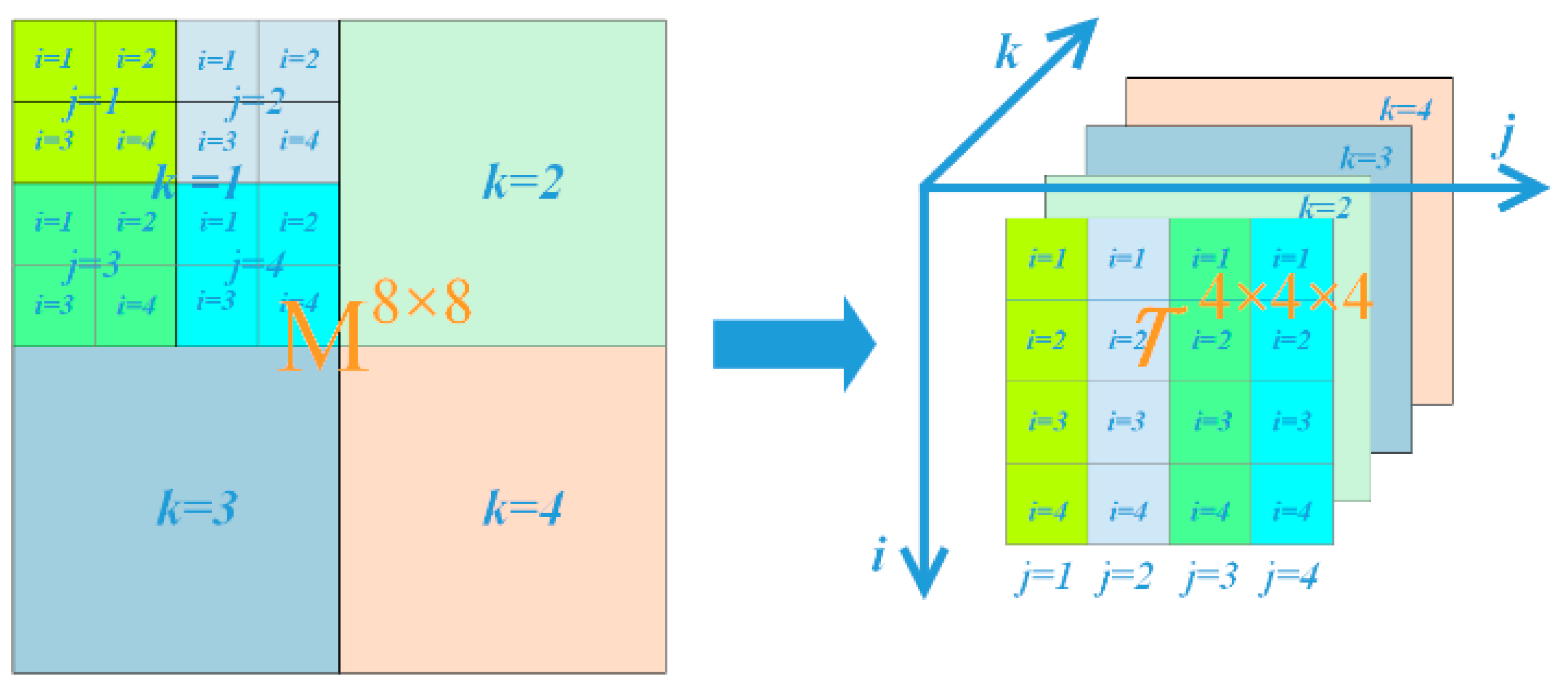
Figure 2.
The t-SVD of a tensor of size I1×I2×I3.
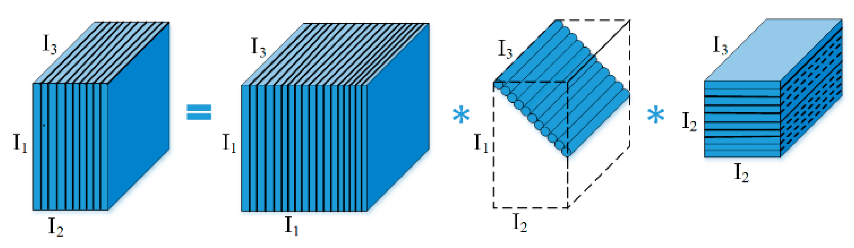
Figure 3.
The tensor train decomposition of an order-N tensor with the size of I1×I2×…×In×…×IN.
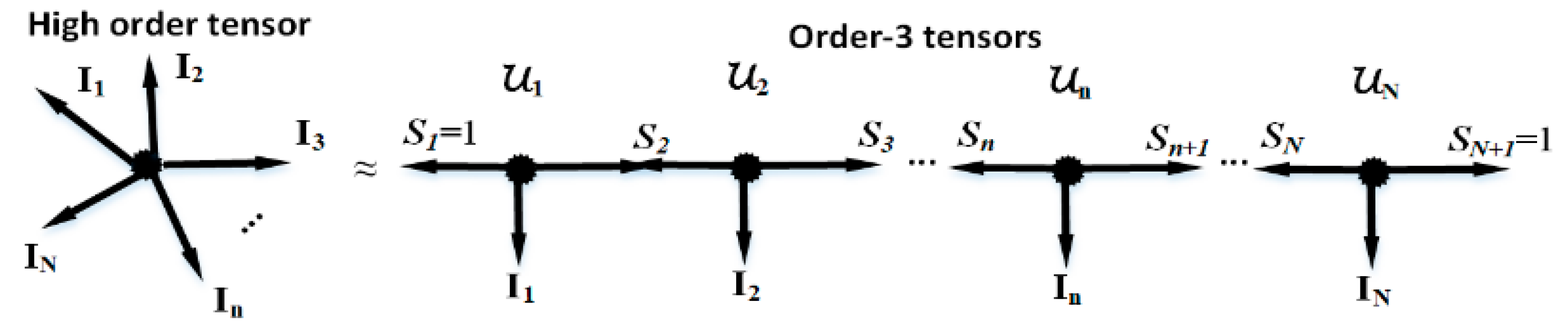
Figure 4.
(a) Examples of the basic QA. By the basic QA scheme, the matrix M size of 8✕8 can be turned into an order-3 tensor with a size of 4✕4✕4. (b) By the basic QA, the Lena image can be divided into 4 small Lena images. (c) The four-pixel values curves of the four smaller Lena images have overlapped into one curve.
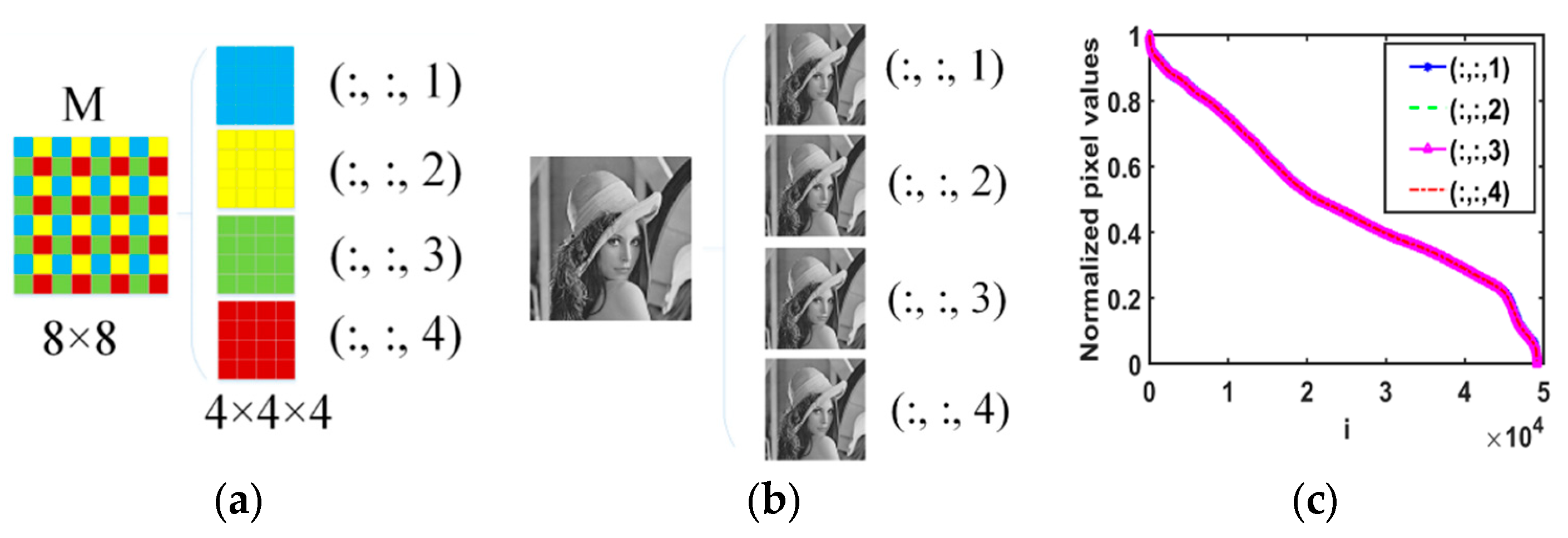
Figure 5.
(a) The first flexible QA scheme to obtain the unfolding matrix. Take the Lena RGB image as an example, we first permute the image size of 256✕256✕3 to order-3 tensor with the size of 32×32×192 by the basic QA scheme. Then this order-3 tensor is reshaped into the unfolding matrix of size 1024✕92. (b) The singular values of this unfolding matrix.
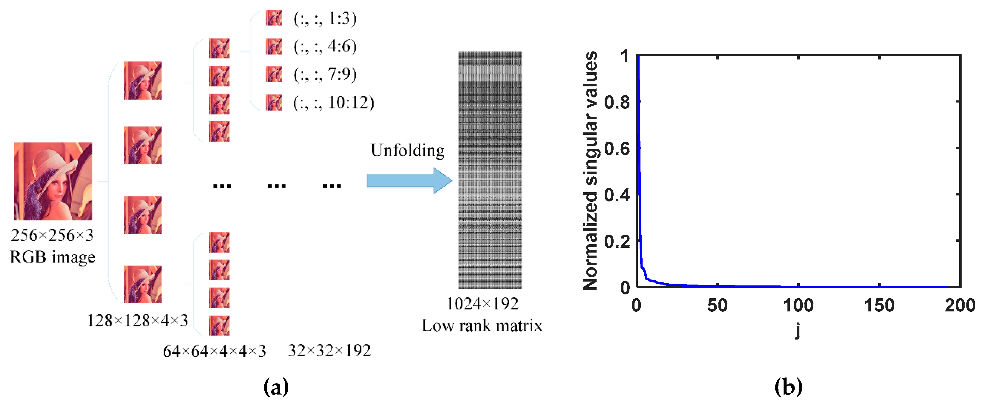
Figure 6.
(a) The second flexible QA scheme to permute the image into a balanced order-3 tensor. Take the Lena image size of 256×256×3 as an example, we obtain the balanced order-3 tensor size of 64×64×48 by multiple QA schemes. This balanced order-3 tensor is more suitable for the t-SVD decomposition than the original image size of 256×256×3. (b) The low tubal rankness of the balanced order-3 tensor.
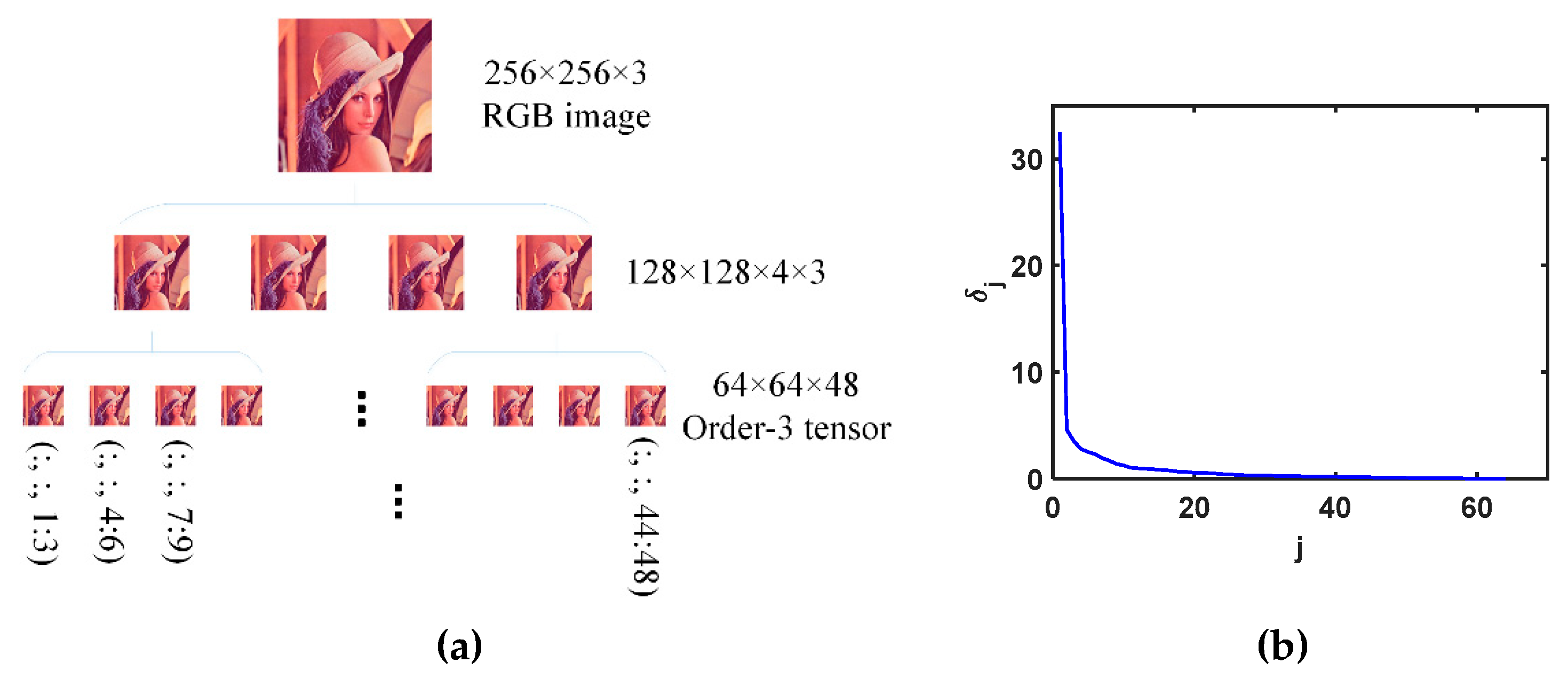
Figure 7.
(a) Examples of the third flexible QA scheme. By the third flexible QA, the matrix size of 16×16 can be permuted into an order-4 tensor size of 4×4×4×4. (b) Singular values of TT matrices. We permute the order-3 Lena RGB image size of 256×256×3 into an 8-order tensor with the size of 4×4×4×4×4×4×4×4×3 by the third flexible QA scheme. Then eight different TT matrices are obtained from this higher-order tensor. We labeled those TT matrices as k=1, 2, …, 8.
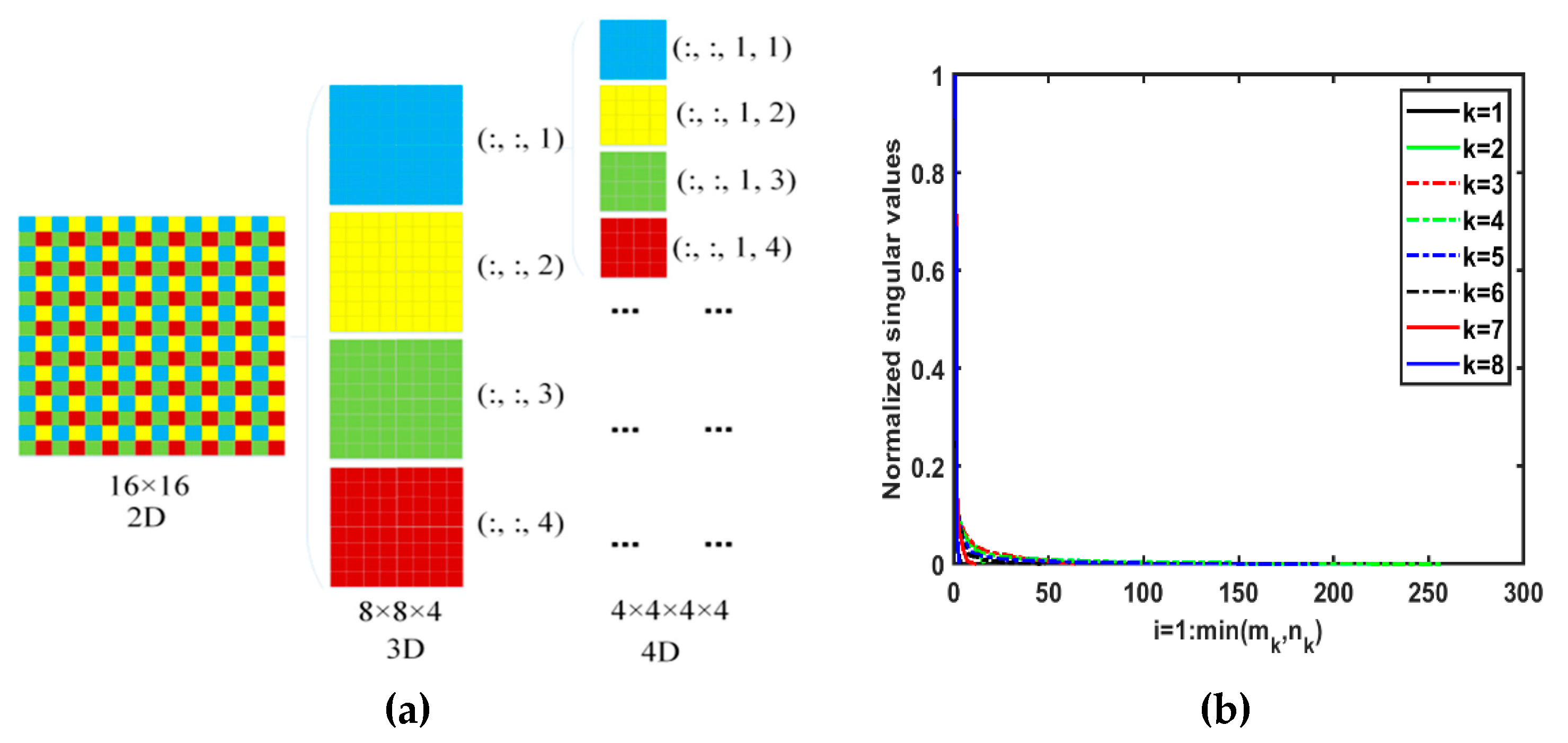
Figure 8.
Original color images and missing patterns.
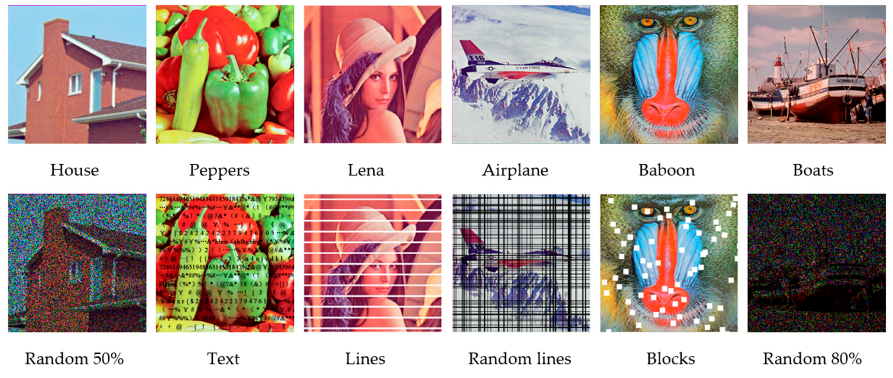
Figure 9.
Comparison of KA and QA scheme under the corresponding TMac-TTKA method [21] and our TTLR method respectively. The first row lists the painted images with a random missing pattern and the missing ratio is 80%. The second row lists the recovered images by TMac-TTKA method. The last row lists the recovered images by LRTT method.
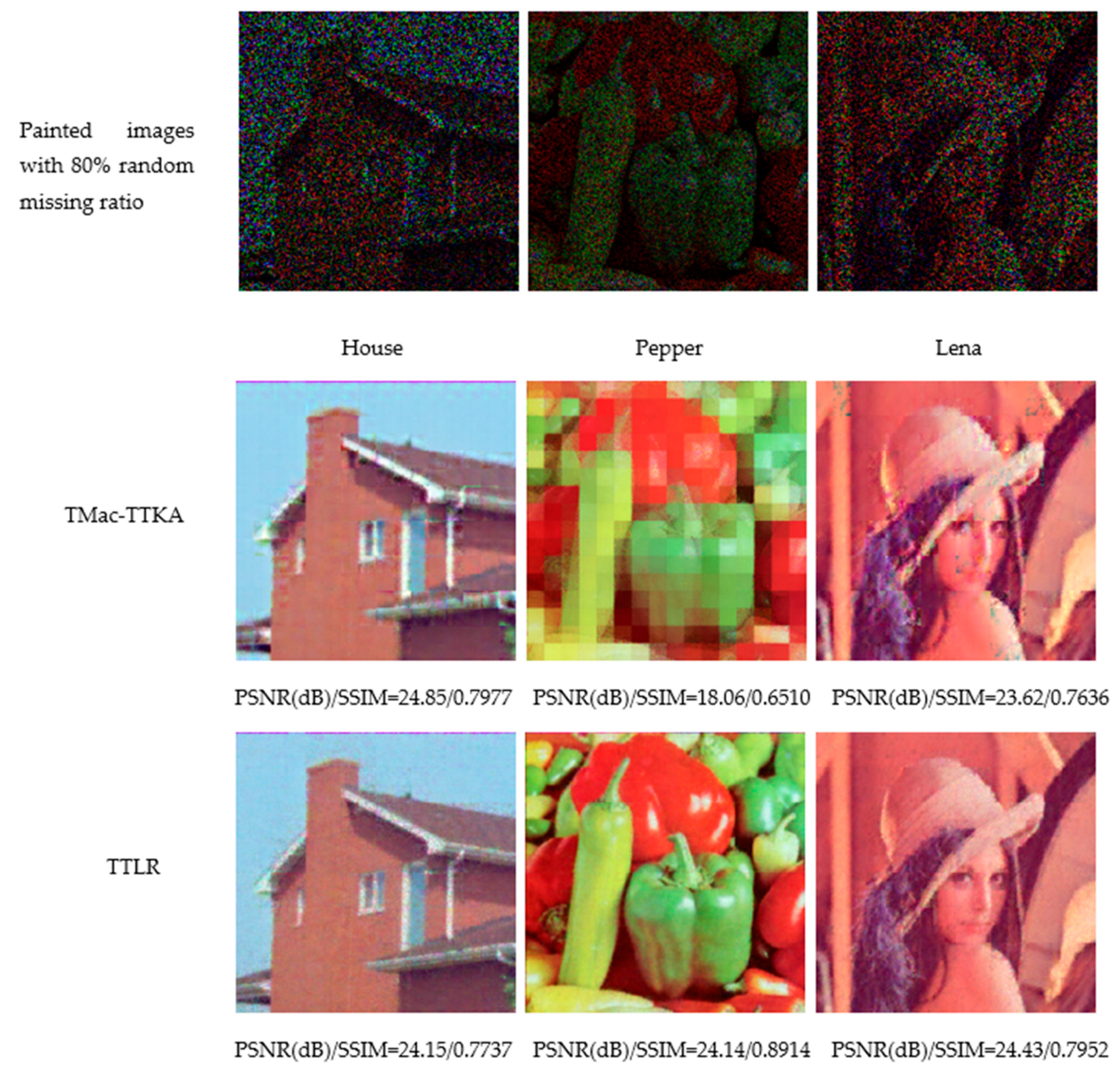
Figure 10.
The missing patterns and inpainting results of House image solved by different methods.
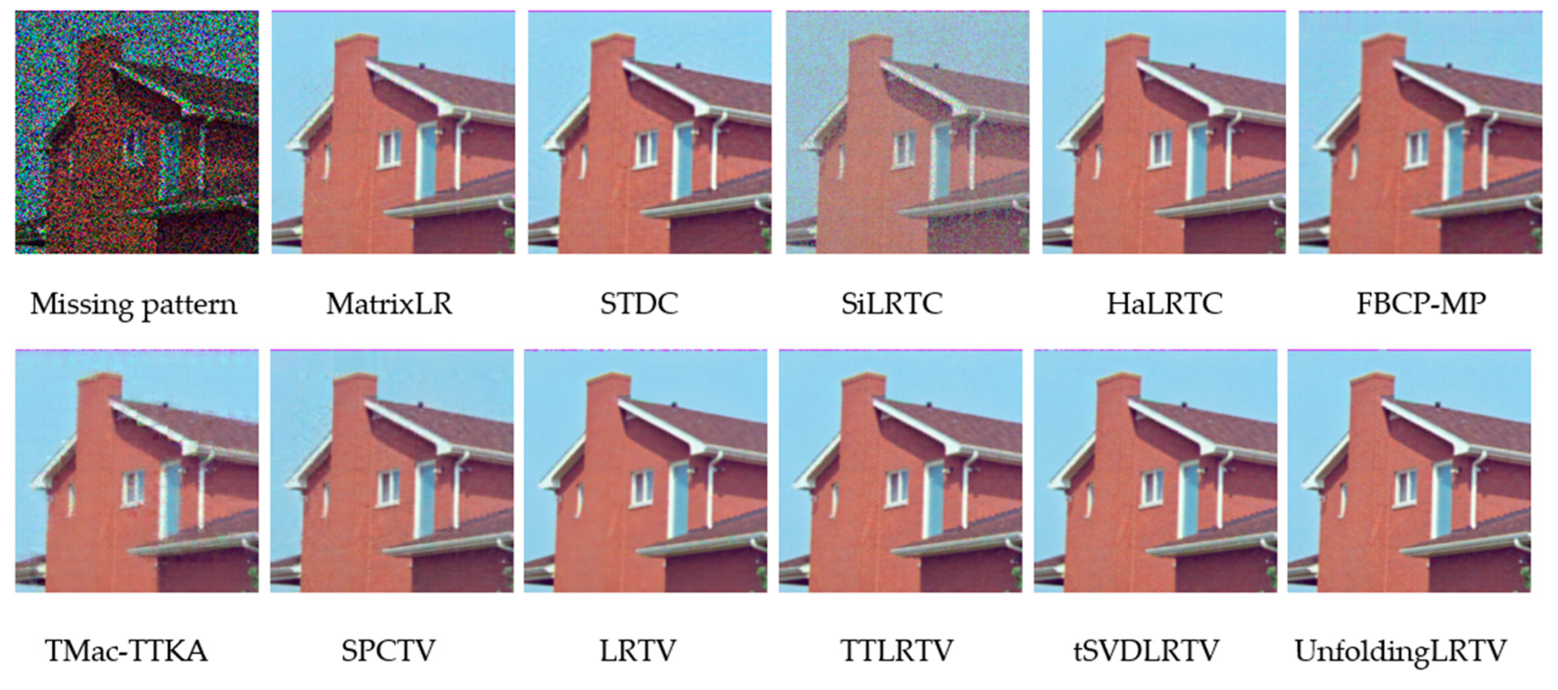
Figure 11.
The missing patterns and inpainting results of Lena image solved by different methods.
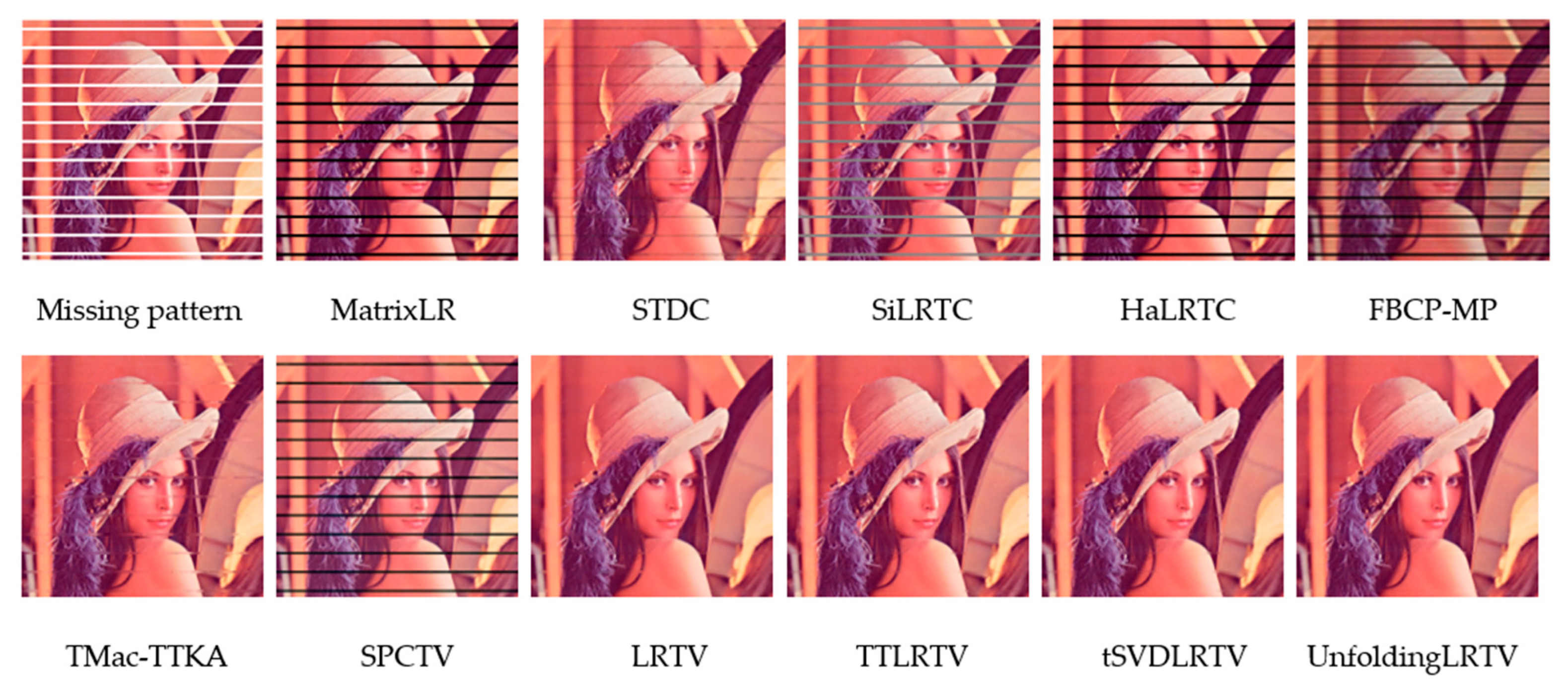
Figure 12.
The missing patterns and inpainting results of Baboon image solved by different methods.
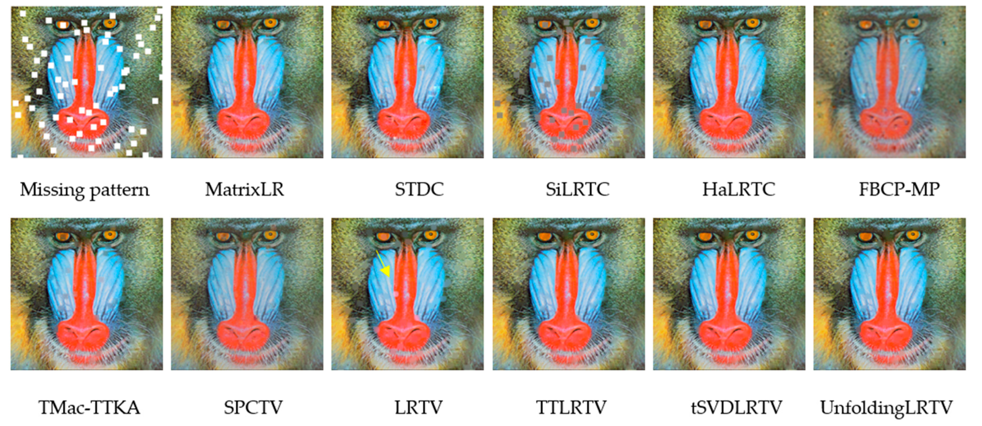
Figure 13.
The PSNR curves of the inpainting results of the six images solved by different methods. The missing ratio ranges from10% to 70% under random missing pattern.
Figure 13.
The PSNR curves of the inpainting results of the six images solved by different methods. The missing ratio ranges from10% to 70% under random missing pattern.
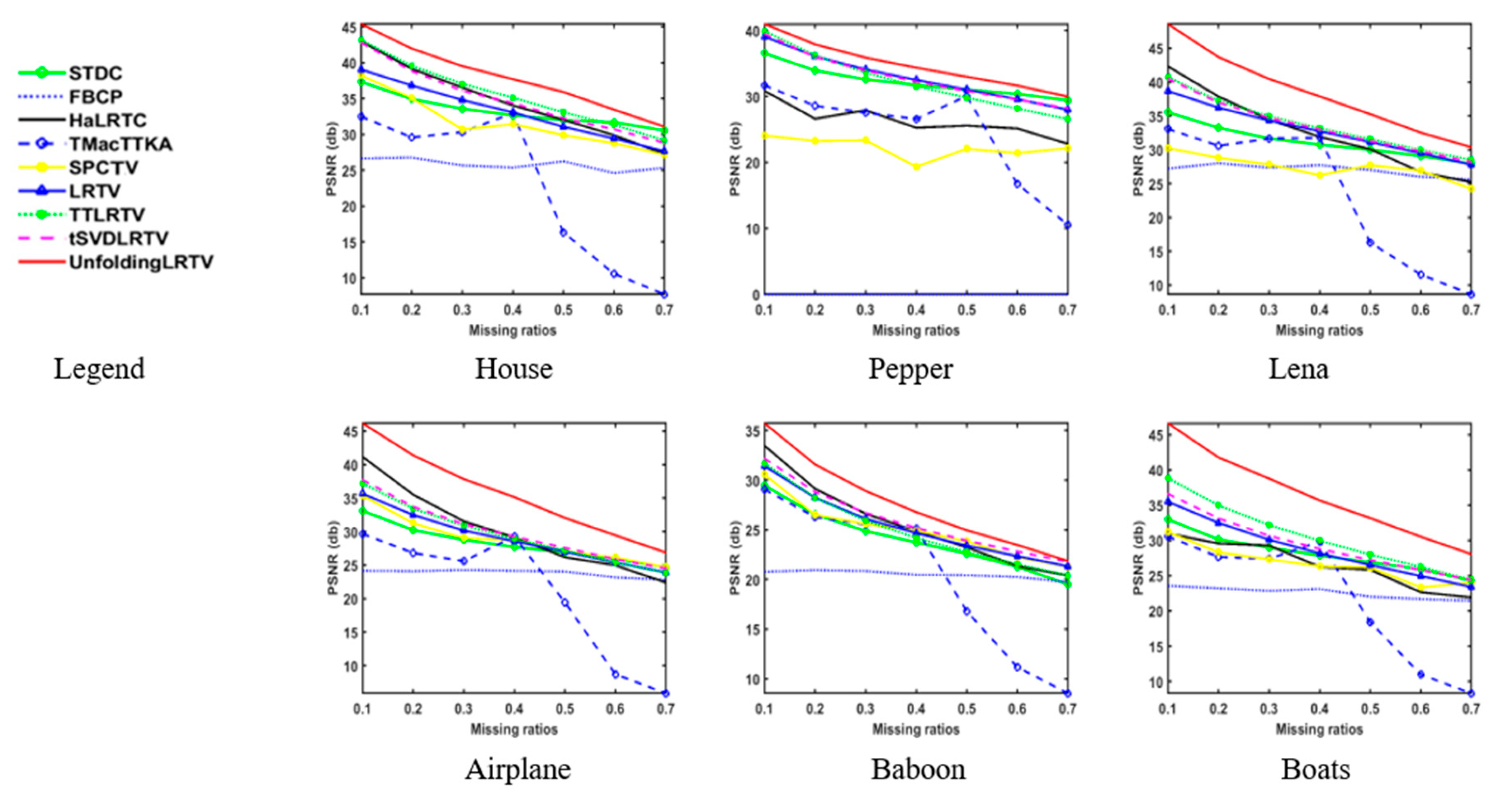
Figure 14.
The visual and numerical PSNR (dB)/SSIM comparisons of our methods for recovering the pepper image under 80% random missing patterns. In the first row, the methods only exploit low-rank constraints. As shown in the color box, there are small blocky errors in the repaired image, this is caused by the QA scheme. This phenomenon can be solved by combining the constraints of low rank and sparsity (TV) as shown in the second row.
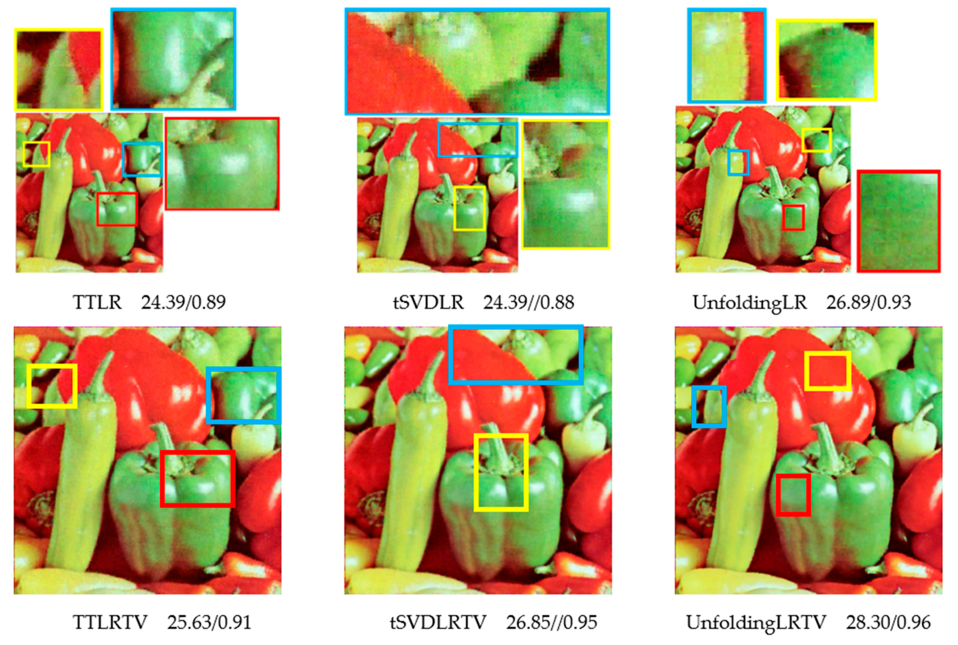
Figure 15.
PSNR (dB) results contributed by each TT matrix in TTLR method and TTLRTV method. We permute the image size of 256×256×3 to an order-9 tensor by the QA scheme. Then we labeled the TT matrices of this order-9 tensor as k=1, 2, …, 8. We use the random missing patterns with four missing ratios: 10%, 30%, 50%, and 70% respectively. The tested color images for the PSNR curves in (a)-(c) are House, Lena and Airplane images respectively.
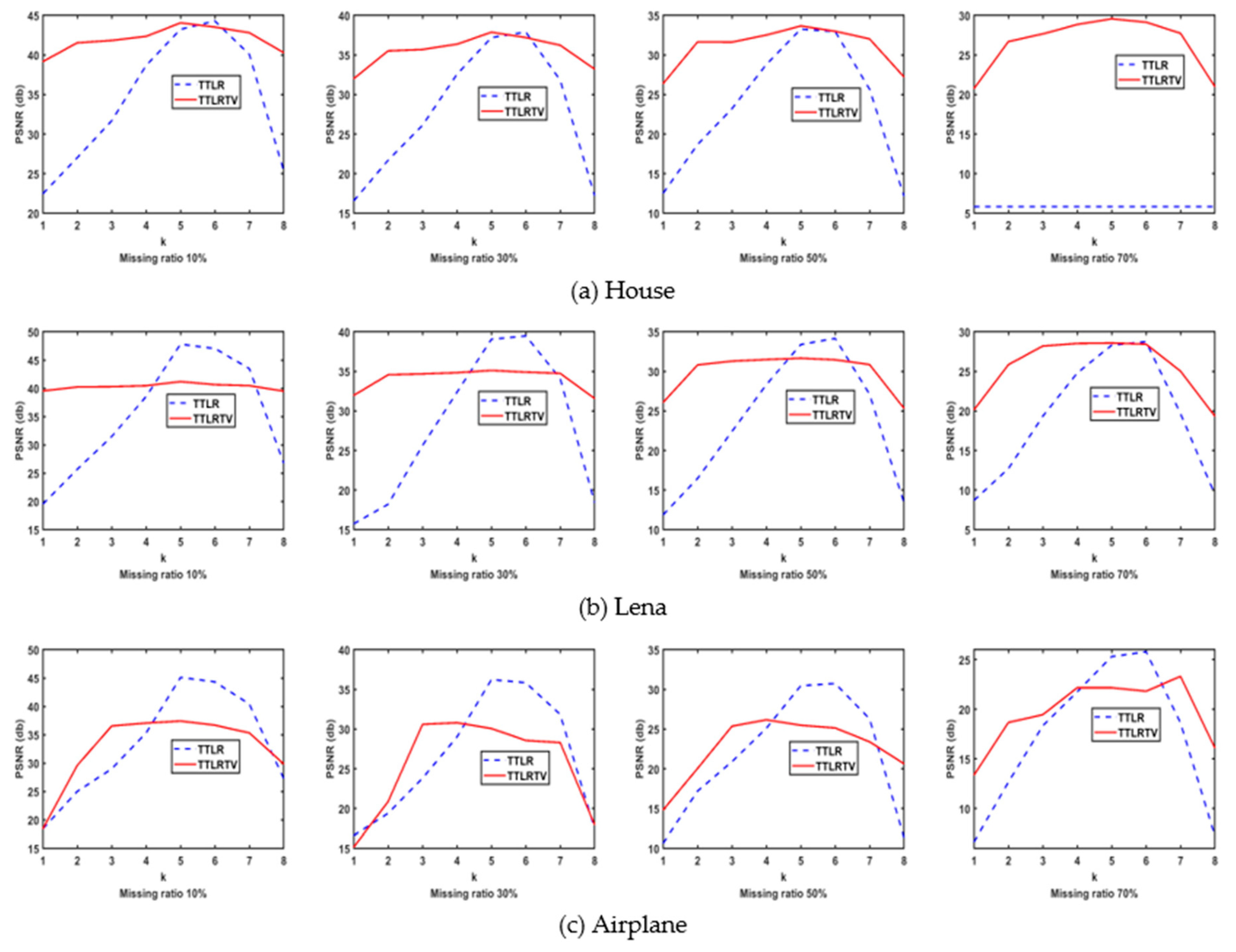

Table 1.
Notations and definitions.
| Symbols | Notations and definitions |
|---|---|
| fiber | A vector defined by fixing every index but one of a tensor. |
| slice | A matrix defined by fixing all but two indices of a tensor. |
| The frontal slice of a 3-order tensor . | |
| Mode-n matrix, the result of unfolding tensor by reshaping its mode-n fibers to the columns of . | |
| f-diagonal tensor | Order-3 tensor is called f-diagonal if each frontal slice is a diagonal matrix [10]. |
| orthogonal tensor | Tensor with the size of is called orthogonal tensor if , where stands for identity tensor if the first frontal slice is the identity matrix and all other frontal slices () are zero. |
Table 2.
Algorithm 1.
| Input: , maximum number of iteration , convergence condition . |
| Initialization: initial , by solving the matrix completion problem (11), , , , t=0. |
|
While and do The first flexible QA scheme: Turn an image into an order-N tensor , then unfold it. Solve (5)-(10) for , where * represents the optimal solution. Update , . End while |
| Output: . |
Table 3.
Algorithm 2.
| Input: , the maximum number of iteration , convergence condition . |
| Initialization: , , , , t=0. |
|
While and do QA scheme: Turn an image into the balanced order-3 tensor . Update Update Update Update , Update , . End while |
| Output: . |
Table 4.
Algorithm 3.
| Input: , the maximum number of iteration , convergence condition . |
| Initialization: , by the LMaFit method [43]; , , . |
|
For n=1 to N-1 do t=0. While and do QA scheme: permute image to order-N tensor . Update Update Update Update Update , Update , . End while End for |
| Output: . |
Table 5.
PSNR (dB)/SSIM and SSIM of the seven methods without rearrangement and with rearrangement.
| Methods | PSNR (dB)/SSIM of different color images under different missing patterns | ||||
|---|---|---|---|---|---|
| House | Lena | Airplane | Boats | ||
| Random 50% | Lines | Random line | Random 80% | ||
| Without Rearrangement | MatrixLR | 9.38/0.8970 | 13.34/0.5850 | 7.118/0.1308 | 19.18/0.5680 |
| TTLR | 28.61/0.871 | 13.34/0.585 | 7.11/0.130 | 19.25/0.519 | |
| tSVDLR | 32.30/0.932 | 13.34/0.585 | 7.11/0.130 | 21.60/0.707 | |
| UnfoldingLR | 7.83/0.093 | 13.34/0.585 | 7.11/0.130 | 6.32/0.102 | |
| With Rearrangement | TTLR | 30.21/0.9251 | 31.79/0.9559 | 25.77/0.8796 | 21.44/0.7144 |
| tSVDLR | 29.79/0.8989 | 31.20/0.9561 | 18.91/0.8386 | 21.34/0.6879 | |
| UnfoldingLR | 32.58/0.9416 | 33.45/0.9771 | 28.75/0.9464 | 23.46/0.8139 | |
Table 6.
PSNR (dB)/SSIM and SSIM of the nine methods.
| No. | Methods | PSNR (dB)/SSIM of different color images under different missing patterns | ||||||
| House | Peppers | Lena | Airplane | Baboon | Boats | |||
| Random 50% | Text | Lines | Random line | Blocks | Random 80% | |||
| Other methods | 1 | STDC | 32.04/0.9300 | 33.61/0.9813 | 28.56/0.8995 | 23.49/0.7756 | 27.01/0.9293 | 21.88/0.7340 |
| 2 | HaLRTC | 32.07/0.9423 | 25.84/0.9496 | 13.34/0.5850 | 19.94/0.6334 | 28.04/0.9397 | 20.56/0.6858 | |
| 3 | FBCP | 26.41/0.8701 | NAN | 14.56/0.5242 | 10.25/0.1954 | 18.71/0.5546 | 20.91/0.6947 | |
| 4 | TMac-TTKA | 23.18/0.8113 | 29.47/0.9681 | 29.93/0.9462 | 20.82/0.7521 | 28.04/0.9429 | 8.83/0.1229 | |
| 5 | SPCTV | 29.56/0.9133 | 23.38/0.9154 | 16.02/0.6107 | 18.58/0.6894 | 24.21/0.9144 | 20.98/0.7254 | |
| 6 | LRTV | 30.93/0.9382 | 36.98/0.9945 | 34.07/0.9724 | 26.82/0.9228 | 27.10/0.9319 | 21.62/0.7541 | |
| Our methods | 1 | TTLRTV | 33.02/0.9579 | 37.27/0.9945 | 34.94/0.9823 | 28.82/0.9561 | 29.46/0.9559 | 22.37/0.7487 |
| 2 | tSVDLRTV | 32.20/0.9550 | 37.49/0.9950 | 34.70/0.9818 | 28.03/0.9507 | 29.56/0.9574 | 22.86/0.8021 | |
| 3 | UnfoldingLRTV | 35.61/0.9689 | 37.72/0.9952 | 34.87/0.9821 | 29.55/0.9639 | 29.59/0.9556 | 25.43/0.8863 | |
Table 7.
PSNR (dB)/SSIM and SSIM of the eight methods.
| No. | Methods | PSNR (dB)/SSIM of different color images under different missing patterns | |||||
| House | Peppers | Lena | Airplane | Baboon | Boats | ||
| Random 50% | Text | Lines | Random line | Blocks | Random 80% | ||
| 1 | MatrixLR | 9.38/0.8970 | 33.23/0.9814 | 13.34/0.5850 | 7.118/0.1308 | 27.62/0.9343 | 19.18/0.5680 |
| 2 | TV | 29.70/0.8816 | 34.14/0.9913 | 29.21/0.9107 | 22.85/0.8463 | 23.18/0.9066 | 20.32/0.6103 |
| 3 | TTLR | 30.21/0.9251 | 34.86/0.9892 | 31.79/0.9559 | 25.77/0.8796 | 25.42/0.9239 | 21.44/0.7144 |
| 4 | tSVDLR | 29.79/0.8989 | 33.86/0.9840 | 31.20/0.9561 | 18.91/0.8386 | 28.03/0.9373 | 21.34/0.6879 |
| 5 | UnfoldingLR | 32.58/0.9416 | 36.86/0.9938 | 33.45/0.9771 | 28.75/0.9464 | 22.22/0.9238 | 23.46/0.8139 |
| 6 | TTLRTV | 33.02/0.9579 | 37.27/0.9945 | 34.94/0.9823 | 28.82/0.9561 | 29.46/0.9559 | 22.37/0.7487 |
| 7 | tSVDLRTV | 32.20/0.9550 | 37.49/0.9950 | 34.70/0.9818 | 28.03/0.9507 | 29.56/0.9574 | 22.86/0.8021 |
| 8 | UnfoldingLRTV | 35.61/0.9689 | 37.72/0.9952 | 34.87/0.9821 | 29.55/0.9639 | 29.59/0.9556 | 25.43/0.8863 |
Table 8.
Runtimes(s) of the different methods.
| Methods | Runtime (s) | |||
|---|---|---|---|---|
| House | Lena | Airplane | Boats | |
| Random 50% | Lines | Random lines | Random 80% | |
| MratrixLR | 4.95 | 0.17 | 0.16 | 5.01 |
| STDC | 5.43 | 5.13 | 5.17 | 5.16 |
| HaLRTC | 8.00 | 0.88 | 0.84 | 6.84 |
| FBCP | 188.32 | 86.45 | 132.09 | 219.33 |
| SPCTV | 19.25 | 16.37 | 16.03 | 17.69 |
| LRTV | 19.08 | 20.17 | 21.04 | 21.05 |
| TTLRTV | 145.5 | 143.2 | 142.6 | 142.3 |
| tSVDLRTV | 15.23 | 15.07 | 15.17 | 15.14 |
| UnfoldingLRTV | 9.49 | 8.53 | 8.69 | 8.72 |
Disclaimer/Publisher’s Note: The statements, opinions and data contained in all publications are solely those of the individual author(s) and contributor(s) and not of MDPI and/or the editor(s). MDPI and/or the editor(s) disclaim responsibility for any injury to people or property resulting from any ideas, methods, instructions or products referred to in the content. |
© 2023 by the authors. Licensee MDPI, Basel, Switzerland. This article is an open access article distributed under the terms and conditions of the Creative Commons Attribution (CC BY) license (http://creativecommons.org/licenses/by/4.0/).
Copyright: This open access article is published under a Creative Commons CC BY 4.0 license, which permit the free download, distribution, and reuse, provided that the author and preprint are cited in any reuse.


