
Submitted:
23 October 2023
Posted:
24 October 2023
You are already at the latest version
Abstract
Changes in sea level exhibit nonlinearity, nonstationarity, and multivariable characteristics, making traditional time series forecasting methods less effective in producing satisfactory results. To enhance the accuracy of the predictions of changes in sea level, this study introduced an improved VMD–EEMD–LSTM hybrid model. This model decomposes satellite altimetry data from near the Dutch coast using VMD, resulting in components of the Intrinsic Mode Function (IMF) with various frequencies and a residual sequence. EEMD further dissects the residual sequence obtained from VMD into second-order components. These IMFs decomposed by VMD and EEMD are utilized as features in the LSTM model for making predictions, culminating in the final forecasted results. The experimental results demonstrated significant improvements in the predictive performance compared with the VMD–LSTM model. The RMSE (root mean square error) decreased by an average of 58.68%, the MAE (mean absolute error) reduced by an average of 59.96%, and the R2 (coefficient of determination) increased by an average of 49.85% compared with the VMD–LSTM model. In comparison with the EEMD–LSTM model, the RMSE decreased by an average of 26.95%, the MAE decreased by an average of 28.00%, and the R2 increased by an average of 6.53%. The VMD–EEMD–LSTM model exhibited significantly improved predictive performance.
Keywords:
sea level change
; deep learning
; time series prediction
; VMD
; EEMD
; LSTM
1. Introduction
In recent years, the continual rise in sea-level has had severe social impacts on coastal areas, including the degradation of freshwater resources, damage to infrastructure, and the depletion of agricultural resources [1,2,3,4,5]. The Sixth Assessment Report of the Intergovernmental Panel on Climate Change (IPCC) highlighted that under the influence of human activities, the rate of the rise in sea level has been steadily accelerating. Between 1901 and 1971, the average rate of the rise in sea level was 1.3 millimeters per year, which increased to 1.9 millimeters per year between 1971 and 2006, and rose further to 3.7 millimeters per year between 2006 and 2018 [6,7,8]. To address the threats posed by rising sea-level, accurate predictions of future changes in sea level are of paramount importance for the sustainable development of coastal regions [7,8,9].
Currently, time series forecasting methods for predicting sea-level primarily fall into two categories: statistical methods and machine learning methods [10,11,12,13,14,15,16]. Statistical methods are widely used in time series forecasting and are rooted in the core concept of conducting statistical analyses on historical data to capture the patterns and trends for predictive purposes [17,18,19,20]. Representative models in this category include ARIMA (auto-regressive integrated moving average) and exponential smoothing [21,22,23,24,25,26]. However, these models face challenges when dealing with complex nonlinear data, as they require manual selection of the features and adjustments of the model’s parameter, leading to some degree of systematic bias and limitations [27,28,29]. Traditional machine learning methods, while capable of automatically extracting features and adjusting the model’s parameters, may not adequately extract the features when dealing with large-scale and highly complex data, resulting in limited predictive performance [30,31]. In contrast, deep learning, as an emerging machine learning technology, has demonstrated a strong capacity for generalization and adaptability to complex data through specific neural network architectures and training methods. It is becoming increasingly prevalent in time series data of sea-level characterized by nonlinearity, non-stationarity, and multivariable attributes. Makarynskyy et al. (2004) utilized artificial neural networks (ANN) to perform multistep predictions based on measured sea level data from a tidal station in Australia, affirming the feasibility of using neural network methods in prediction sea-level [32]. Balogun and Adebisi (2021) conducted comprehensive predictions and comparisons of changes in sea level along the west coast of Peninsular Malaysia using three models: ARIMA, support vector regression (SVR), and long short-term memory (LSTM). Their research findings validated the superiority of the LSTM model in predicting sea-level [33].
With the continued advancement of deep learning methods in the field of time series forecasting, various domains of time series prediction have witnessed the superior predictive accuracy achieved by combining data decomposition techniques with deep learning, as supported by research findings [34,35,36]. Song et al. (2022) conducted multifaceted comparisons of various data decomposition methods, such as complementary ensemble empirical mode decomposition (CEEMD), time-varying filtering-based empirical mode decomposition (TFV–EMD), wavelet transform (WT), and the fusion of these methods with the Elman neural network (ENN) in minute-scale time series predictions of sea level. Their study confirmed that the TVF–EMD–ENN model exhibits the best predictive performance [37]. Wang et al. (2021) incorporated time series of wind speed that had been secondarily decomposed using CEEMD and wavelet packet decomposition (WPD) into a gated recurrent unit (GRU) for making predictions. Their experiments demonstrated that this hybrid model significantly improved the accuracy of short-term wind speed predictions [38]. Variational mode decomposition (VMD), as an emerging data decomposition technique, has stood out among the various decomposition methods due to its unique non-recursive variational approach and exceptional decomposition capability. It has been widely applied in the field of mixed deep learning time series prediction [39,40]. Wang et al. (2020) combined the VMD–LSTM model and used an improved particle swarm optimization algorithm (IPSO) to optimize model parameters, confirming the higher predictive accuracy of the VMD–LSTM model in photovoltaic short-term power time series prediction [41]. Huang et al. (2022) conducted a comparison between Empirical Mode Decomposition (EMD) and VMD, revealing that VMD exhibited stronger noise removal capabilities. They also verified the higher precision of the VMD–LSTM model in predicting variations in coal thickness [42]. Han et al. (2019) performed multifaceted comparisons of various prediction models, including VMD–LSTM, Persistence (PER), Wavelet (WT), and BP neural networks. Their research validated that the VMD–LSTM model exhibited higher accuracy in wind power prediction [43].
The aforementioned studies across various time series domains have consistently demonstrated the superior predictive accuracy of the VMD–LSTM model. However, in practical applications, due to variations in VMD parameter settings and data characteristics, incomplete VMD decomposition may occur. This results in residual components that still contain a certain level of fluctuations and nonwhite noise elements. This inadequately processed information can potentially have a detrimental impact on the predictive accuracy of the VMD–LSTM model, particularly in forecasting complex nonlinear and irregular time series. In light of these challenges, this study proposed a deep learning hybrid model based on the VMD–LSTM model, known as the VMD–EEMD–LSTM model, which incorporates both VMD and ensemble empirical mode decomposition (EEMD). This model aims to enhance the predictive accuracy of the VMD–LSTM model for sea level time series by further processing the residual sequences obtained from VMD decomposition. Evaluation of the VMD–EEMD–LSTM model's predictive performance was conducted with multiple models, various perspectives, and multiple monitoring stations for a comprehensive validation.
2. Principles and Methods
2.1. Signal Processing Methods
VMD, EMD, EEMD, and CEEMDAN (Conformal Empirical Mode Decomposition with Adaptive Noise) are all widely used adaptive methods of data decomposition in the fields of signal processing and data analysis [44,45,46]. Among them, VMD is a completely non-recursive modal decomposition method. Its core idea involves modeling a signal as a variational problem and subsequently seeking the optimal solution through iterative transformations. Ultimately, this process decomposes nonstationary signals into a series of standard orthogonal modal functions. The corresponding principles are as follows [47,48].
(1) With the objective of minimizing the summation of the estimated bandwidths for each modal component , a constrained variational problem model aimed at identifying the optimal solution. The specific formulation of the constrained variational problem model is provided below.
In Equation 1, , represents the Dirac function, corresponds to the modal functions obtained after decomposition, denotes the central frequencies associated with each mode, and represents the original signal.
To attain the optimal solution for the constrained variational problem, the introduction of quadratic penalty factors and Lagrange multiplier operators transforms the problem into an unconstrained variational problem.
where represents the augmented Lagrangian function, is the quadratic penalty term. Subsequently, an alternatively direction method with multiplier operators is used to solve the unconstrained variational problem, and the optimal solution is obtained by alternating updating , , and .
As a recursive method, the EMD method decomposes the data into a finite number of intrinsic mode functions (IMF) that reflect the inherent properties of the time series signals, along with a "residual sequence" [49,50]. However, the EMD may suffer from the mode-mixing problem in the IMF sequences. To overcome this challenge, this study introduced the EEMD method. EEMD gradually introduces normally distributed white noise into the original signal and then offsets this noise through multiple averaging calculations. This process leads to more precise decomposition of the signal and effectively avoids the mode mixing phenomenon that can occur during the EMD decomposition process [51,52,53]. The specific process is as follows:
(1) Initially, white noise denoted as is introduced into the original signal.
(2) Subsequently, the EMD method is employed to decompose the initial noisy signal, resulting in n IMF, represented as , and a residual sequence represented as .
(3) Steps (1) and (2) are iteratively executed for a total of times, in which white noise is added and IMF components are obtained through decomposition in each iteration. Finally, all the IMF components thus obtained are integrated and averaged to obtain the ultimate result of EEMD signal decomposition.
CEEMDAN introduces an adaptive noise complete set to automatically construct noise components, enabling more effective extraction of modal components in the signal compared to EEMD. This enhances the accuracy and robustness of data decomposition [54].
2.2. Long Short-Term Memory
LSTM is an improved type of recurrent neural network (RNN). Its distinctive memory module is beneficial for handling long-term dependencies and mitigating the challenges related to vanishing and explosion gradients [55]. Compared with traditional neural networks, LSTM networks exhibit pronounced advantages when addressing tasks pertaining to the prediction of lengthy time series data. Consequently, LSTM networks find extensive applications in domains such as time series forecasting [56,57].
The architectural framework of LSTM network comprises an input layer, intermediate hidden layers, and an output layer. Each hidden layer controls storage and access of the data through input gates, forget gates, and output gates, as visually depicted in Figure 1.
As illustrated in the figure, LSTM processes the input of high-temporal data related to sea surface elevation and the previous moment's hidden state output using three gates. The primary process is as follows:
(1) LSTM, through the forget gate (denoted as ), determines whether to discard or retain information related to and is governed by the activation function of the forget gate.
In the equations, and represent the weight matrices and biases, respectively. is a vector with values in the range of 0 to 1, where the values within the vector indicate whether information in the cell state is preserved. A value of 0 implies no preservation, while 1 implies full preservation.
(2) The cell state is updated through the input gate by passing and to the activation function to determine the information update. and are passed to the tanh function to create a new candidate value vector (where is a vector in the range of -1 to 1), and the tanh output is multiplied by output.
(3) The cell state from the previous layer is element-wise multiplied with the forget vector, and then this value is element-wise added to the output of the input gate, resulting in the updated cell state.
In the equations, determines the forgetting of information in , while determines the addition of information in to the new memory cell state .
(4) Through the output gate , the value of the next hidden state is determined, and this hidden state contains information from previous inputs.
2.3. The VMD–EEMD–LSTM Hybrid Second-Order Decomposition Prediction Model
VMD and EEMD, as two classical data processing methods, have been widely applied in hybrid modeling. Their effectiveness in enhancing the predictive accuracy of deep learning models has been well-established [58,59,60,61]. The VMD–LSTM model, as a prevalent hybrid deep learning approach, has been widely employed in the realm of time series forecasting. Its applications encompass load forecasting and wind speed prediction, where it has showcased remarkable performance [62,63]. The VMD–LSTM model leverages VMD to perform decomposition of the initial data into a sequence of IMF sequence and a residual sequence. Subsequently, the model individually forecasts each IMF sequence and the residual sequence using the LSTM model. Ultimately, the predicted outcomes of each sequence are aggregated to derive the final model prediction. During the prediction process, as the standard normal mode functions obtained through VMD decomposition are stationary signals, predicting each IMF separately can achieve higher prediction accuracy. However, in practical VMD decomposition, the residual sequence still contains some fluctuating characteristics and high-frequency noise, and their values are relatively large. If these parts of the data are not appropriately processed, they will adversely affect the overall predictive accuracy of the model [64,65,66]. In contrast, the EEMD–LSTM model is a recursive decomposition method, and its main predictive errors are concentrated in the IMF components, which perform well in predicting the residual sequence and overall data. Based on this, this study proposed a deep learning hybrid model called VMD–EEMD–LSTM. This model employs VMD for the initial data decomposition and then utilizes EEMD to further break down the residual components with lower prediction accuracy resulting from the VMD decomposition. Subsequently, each IMF obtained through both VMD and EEMD decomposition is used as a feature used as input into the LSTM model for making predictions. Ultimately, the forecasted outcomes of each IMF are aggregated to yield the model's comprehensive prediction. This approach augments the overall predictive precision of the model by handling the residual components produced by VMD. The detailed procedure is elucidated in Figure 2.
The specific prediction process of the mixed VMD–EEMD–LSTM second-order decomposition model is as follows.
Step 1: Preprocess the time series data on sea level from each station and then input them into the VMD model (with K as the number of components in the model) for decomposition.
Step 2: Take the residual sequence "Residual 1" obtained from the VMD decomposition, and input it into the EEMD model for further decomposition. This will yield various model components as well as "Residual 2".
Step 3: Through extensive experiments, it has been determined that among the IMF components obtained through EEMD decomposition, the IMFs after IMFK (IMF K+1 to IMF n) and "Residual 2" have smaller prediction errors. To mitigate experimental intricacies and guarantee the precision of the model's predictions, the IMF components beyond IMF K and 'Residual 2' are combined and utilized as input features for the LSTM model to facilitate the prediction process.
Step 4: Utilizing the distinct IMF components acquired from both VMD decomposition and the EEMD decomposition as distinct features, these components are fed into the LSTM model for prediction purposes. This process yields a total of 2K+1 predictions.
Step 5: Aggregate and amalgamate the 2K+1 predictions to derive the ultimate prediction generated by the VMD–EEMD–LSTM model.
2.4. Evaluation index
To evaluate the precision and dependability of the diverse deep learning models in predicting performance, this study employs the subsequent assessment metrics: RMSE (root mean square error), MAE (mean absolute error), and R2 (Coefficient of determination). The definitions of these three-evaluation metrics are elaborated as per references [67,68,69]:
- (1)
- RMSE
- (2)
- MAE
- (3)
- R2
where represents the actual values of sea level, represents the values predicted by each model, is the mean of the actual values of sea level, and n denotes the total number of data points related to sea level. For RMSE and MAE, smaller values indicate higher predictive accuracy, while for R2, values closer to 1 indicate accurate predictions, and values closer to 0 suggest that the model has weaker explanatory power.
To visually assess the enhanced performance of the VMD–EEMD–LSTM model in comparison to other hybrid models across diverse accuracy evaluation metrics, this study introduces the concept of an improvement ratio (I). Through the computation of I, the degree of enhancement achieved by the VMD–EEMD–LSTM model in terms of accuracy can be precisely quantified. The formula for calculating I is defined as follows:
where y and signify diverse evaluation metrics, y represents the evaluation metric of the hybrid models compared against the VMD–EEMD–LSTM model, while represents the evaluation metric of the VMD–EEMD–LSTM model. If is greater than 0, it indicates a decreasing trend in the accuracy. If is less than 0, it indicates an increasing trend. The greater the absolute value of , the greater the improvement in that evaluation metric for the hybrid model and vice versa.
3. Data and experiments
3.1. Data Preprocessing
The satellite altimetry grid data used in this study were obtained from the European Union's Copernicus Earth Observation Program, specifically from the GLORYS12V1 product (GLOBAL_MULTIYEAR_PHY_001_030). The data have a spatial resolution of 0.083° × 0.083° and a temporal resolution of 1 day [70]. The GLORYS12V1 product is a reanalysis of the global ocean with a 1/12° horizontal resolution and 50 vertical levels, covering sea level measurements from 1993 onwards. It has undergone the necessary standard corrections. To ensure the fairness of the experiments, this study utilized data from six satellite altimetry grid points near the coast of the Netherlands. All the selected data have a consistent temporal coverage, spanning from early 1993 to the end of 2020, totaling 28 years. The distribution of the data is presented in Table 1.
3.2. Experimental pretreatment
3.2.1. Parameter Settings of VMD
Unlike EMD and EEMD, VMD allows for the autonomous selection of the number of mode components obtained during decomposition.
Therefore, in the context of utilizing VMD for data decomposition, the choice of an appropriate number of mode components, denoted as K, is of paramount importance to attain high-quality decomposition outcomes. Opting for a K value that is excessively large may lead to over-decomposition, whereas selecting one that is overly small may result in under-decomposition. To ascertain the optimal K value for the sea level height time series post-decomposition, this investigation employs the signal-to-noise ratio (SNR) as an evaluative criterion for decomposition quality. A higher SNR corresponds to a more distinct signal decomposition and improved noise removal. Following comprehensive experimental inquiry and empirical observations, this study confines the selection of K values to the range of 2 to 10, and identifies the K value within this range that yields the highest SNR as the optimal K value for each individual time series [71,72].
where represents the original signal, and represents the reconstructed signal. In VMD, the penalty factor α also exerts a certain influence on the decomposition outcomes. Given that the optimal range for the penalty factor α is typically between 1.5 and 2 times the size of the decomposed data [73], and to ensure experimental consistency while considering the size of the decomposed data in the experiments, this study set the penalty factor to 15,000 for all decomposition processes.
Because the range of sites covered in this study was relatively small, the frequency of fluctuation and the amplitude of the sequences of sea level height were quite similar. Therefore, the optimal parameters obtained in the experiments were consistent, all indicating that K=5 was the best number of components for decomposition (Figure 4 in Section 4.2 shows the results VMD decomposition for K=5). To reduce the complexity of the subsequent experiments and ensure experimental consistency, this study combined the data with a K greater than 5 from the IMF obtained by EMD and EEMD decomposition with the residual term for a better predictive analysis.
To further validate the reliability of the selected K value, the LSTM model was employed to conduct comparative experiments for sea level data prediction at the Maassluis station. The experimental results are presented in Table 2.
As presented in Table 2, distinct values of K in VMD decomposition produce residual sequences that manifest substantial predictive errors, constituting the primary source of discrepancies within the VMD-LSTM model. A comparative analysis of predictive outcomes across varying K values reveals that with the escalation of K, the R2 for residual sequence predictions gradually diminishes, while the cumulative errors for each IMF increase. This observation implies that the selection of an excessively diminutive K value may result in an inadequate decomposition of the signal, ultimately yielding inferior predictive performance. Conversely, opting for an excessively large K value may lead to an exorbitant decomposition of the signal, which is also not conducive to model prediction.
When K is set at 5, the VMD-LSTM model attains the highest level of predictive accuracy. This reaffirms that, in the context of time series prediction for sea level data, K=5 represents the optimal number of decompositions for VMD.
3.2.2. Parameter Settings of the Model
In deep learning prediction models, a variety of different parameters are involved, and the sizes of the parameters have different degrees of influence on the model’s predictive accuracy. In order to ensure the reliability, this study conducted an experiment by setting the same model parameters. The configuration details of each model are presented in Table 3. In this experimental setup, the parameters for the LSTM model and the hybrid models were set to identical sizes.
According to Table 3, all models employed a uniform data partitioning scheme in this research: the data spanning from early 1993 to the end of 2012 constituted the training set, data from the end of 2012 to the end of 2015 served as the validation set, and data from the end of 2015 to the end of 2020 comprised the test set. This data splitting approach was adopted with the intention of ensuring that the models had access to a sufficient volume of training data to thoroughly grasp the underlying data characteristics. Additionally, employing a substantial dataset for testing purposes enabled a more comprehensive assessment of the model's predictive performance.
4. Results and analysis
4.1. Analysis of the predictions of a single deep learning model
In this section, the predictive performance of four different models, namely ANN [74,75], RNN [76,77], gated recurrent units (GRU) [78,79], and LSTM, was comprehensively evaluated and compared using three different sequences of sea level height. The goal was to determine the best-performing model in terms of time series forecasting, providing a reliable foundation for constructing the subsequent hybrid models. The precise evaluation metrics for the predictions of each model are shown in Figure 3.
As shown in Figure 3, for the three different time series datasets of sea level height, the ANN model exhibited the poorest predictive performance, with an average RMSE of 150.85 mm, an average MAE of 114.06 mm, and an average R2 of 0.28 across the different monitoring stations. In contrast, the LSTM model performed the best, with an average RMSE of 137.92 mm, an average MAE of 100.13 mm, and an average R2 of 0.40 across the different monitoring stations. LSTM outperformed ANN, RNN, and GRU, demonstrating its superiority. However, since LSTM is a single model, it failed to fully extract the features of the data during training, resulting in a relatively high RMSE and MAE and a relatively low R2 for the predictions. This phenomenon highlights the challenge that single models face in accurately capturing all the fluctuations and trends in time series data, especially in complex time series forecasting tasks. Therefore, in the subsequent work of constructing the hybrid models, it is necessary to combine the characteristics of the data decomposition methods to further improve the predictive accuracy of the models.
4.2. Analysis of the hybrid deep learning first-order decomposition model
In response to the issue of insufficient extraction of the features of the data by single models in complex time series forecasting, this study introduced and compared four different data decomposition methods: VMD, EMD, EEMD, and CEEMDAN. Taking the original sea level data from the MAASSLUIS station as an example, these methods decomposed the data into multiple IMFs and a residual sequence. Subsequently, the decomposed sequences were used as the model’s features and individually fed into the LSTM model for making predictions. The results for each IMF and residual sequence are shown in Figure 4 and Figure 5. This experiment aimed to gain a deeper understanding of how the different data decomposition methods impact the performance of the LSTM model, and evaluated their potential for improving the accuracy of time series predictions.
In Figure 4 and Figure 5, the “Residual” presented for EMD, EEMD, and CEEMDAN refers to the results obtained by adding up the various IMFs after IMF5 and the residual sequence. From the figures, it can be observed that the IMFs obtained after VMD decomposition have well-defined frequency signals and waveform characteristics. Therefore, the LSTM model produced excellent predictions for each IMF. However, the residual sequence generated after VMD decomposition was relatively large and contained a significant amount of white noise. Consequently, even though there were some waveform features and patterns in the residual sequence, they were challenging for the LSTM model to capture, resulting in less accurate predictions, subsequently affecting the overall accuracy of the VMD–LSTM model’s predictions. In contrast, the EMD, EEMD and CEEMDAN methods, while not performing as well as VMD for predicting the various IMFs, yielded better prediction results for the residual sequence. To further analyze the accuracy of the predictions, this study summarized the evaluation metrics of each hybrid model's results, as shown in Table 4.
From the data in Table 4, it becomes apparent that the EEMD–LSTM model achieved the highest overall predictive accuracy, followed by the EMD–LSTM model and the CEEMDAN model, while the VMD–LSTM model exhibited the lowest predictive accuracy. However, it is noteworthy that a significant portion of the prediction errors in the VMD–LSTM model stemmed from the predictions of the residual sequence, and the prediction errors for the various IMFs were notably lower than those of the EMD–LSTM, EEMD–LSTM and CEEMDAN models.
Although the EEMD-LSTM model may have lower predictive accuracy for the residual sequence compared to the EMD-LSTM and CEEMDAN models, it excels in IMF prediction accuracy and overall accuracy. The CEEMDAN decomposition method, despite its enhanced robustness and applicability compared to EMD, yields predictive accuracy similar to that of the EMD-LSTM model. This indicates that the CEEMDAN-LSTM model does not significantly improve predictive performance in high-resolution sea level data compared to the EMD-LSTM model.
While the EEMD–LSTM model did not perform as strongly as the EMD–LSTM model in forecasting the residual sequence, it outperformed the EMD–LSTM model in forecasting the IMFs. As a result, the VMD–LSTM model excelled in IMFs prediction, whereas the EEMD–LSTM model exhibited the highest overall predictive accuracy. Building upon these insights, this study introduced the VMD–EEMD–LSTM model, which enhances overall predictive accuracy by reprocessing the residual components obtained from VMD decomposition with EEMD in addition to the VMD–LSTM model.
5. Discussion
5.1. Analysis of the predictions of the mixed VMD–EEMD–LSTM second-order decomposition model
To comprehensively evaluate the predictive performance of the VMD–EEMD–LSTM model relative to the VMD–LSTM and EEMD–LSTM models, this study conducted comparative experiments using sea level data from six different monitoring stations (Maasluis, Vlissingen, Hoek Van Holland, Delfzijl, Harlingen, Ijmuiden). In this section, Maaluis station is taken as an example to analyze the differences in the predictions of the hybrid models. To distinguish the models’ results more clearly, this section introduces the prediction error R and analyzes the differences between the original data and the predictions of each hybrid model. The comparative results are shown in Figure 6.
As depicted in Figure 6, the VMD–LSTM model, while reasonably aligning with the overall trend of sea level fluctuations, exhibited suboptimal performance near extreme points, particularly in proximity to local maxima. This observation suggests that the VMD–LSTM model struggled to capture the nuanced characteristics of sea level fluctuations, leading to notable prediction errors. In contrast, the EEMD-LSTM model's predictions closely match the original data, notably in capturing the amplitude of fluctuations, which significantly outperformed those of the VMD–LSTM model. Nevertheless, on a comprehensive scale, the results achieved by the EEMD–LSTM model still lagged behind those of the VMD–EEMD–LSTM model. This indicates that the VMD–EEMD–LSTM model not only represents an enhancement over the VMD–LSTM model but also surpasses the EEMD–LSTM model in predictive accuracy. It underscores the effectiveness of this hybrid model in combining the predictive strengths of the VMD–LSTM and EEMD–LSTM models, resulting in superior outcomes and overall improved predictive performance.
5.2. Analysis of the accuracy of the predictions of the mixed VMD–EEMD–LSTM second-order decomposition model
To gain a more precise insight into the enhancement achieved by the VMD–EEMD–LSTM model in comparison to the VMD–LSTM and EEMD–LSTM models across diverse time series, this section scrutinizes the RMSE, MAE, and R2 of the predictions made by the three hybrid models for sea level time series data collected from six different stations. The evaluation metrics used to gauge the precision of each hybrid model's predictions are depicted in Figure 7, while the improvement ratios of the VMD–EEMD–LSTM model relative to the VMD–LSTM and EEMD–LSTM models for various evaluation metrics are detailed in Table 4.
Figure 7 clearly demonstrates that both the VMD-EEMD-LSTM model and the EEMD-LSTM model exhibit markedly superior predictive accuracy in comparison to the VMD-LSTM model. Furthermore, the VMD-EEMD-LSTM model showcases a noticeable degree of enhancement over the EEMD-LSTM model. The three hybrid models consistently demonstrated similar performance when predicting accuracy across various stations. This suggests that the sea level heights observed at the selected stations in the Netherlands displayed a degree of consistency, resulting in relatively minor variations in prediction accuracy. However, in comparison to the VMD–EEMD–LSTM model, the EEMD–LSTM model exhibited some fluctuations in the evaluation metrics across different time series predictions. This signifies that the stability and accuracy of the EEMD–LSTM model in forecasting results for diverse time series are not as robust as those of the VMD–EEMD–LSTM model. This result underlines the superiority of the VMD–EEMD–LSTM model in handling time series from different stations and, to some extent, validates its ability to adapt more stably to various requirements and scenarios of prediction.
To further evaluate the degree of improvement of the VMD-EEMD-LSTM model over the EEMD-LSTM model and the VMD-LSTM model across various accuracy assessment metrics, this study introduces the concept of an improvement ratio (I) for in-depth analysis. The results are presented in Table 5.
Table 5 provides clear evidence that the VMD–EEMD–LSTM model significantly improved prediction accuracy when compared to the EEMD–LSTM model across various stations. On average, it achieved a remarkable 26.95% reduction in RMSE, a 28.00% reduction in MAE, and a 6.53% increase in R2. The EEMD–LSTM model showed a relatively modest increase of only 6.53% in the R2, indicating that it could fit the actual distribution of the data well. The limited improvement in R2 for the EEMD–LSTM model also indirectly confirmed the high predictive accuracy and superior performance of the VMD–EEMD–LSTM model.
Compared with the VMD–LSTM model, the VMD–EEMD–LSTM model exhibited even more significant improvements in the accuracy of its prediction, with an average reduction of 58.68% in the RMSE, an average reduction of 59.96% in the MAE, and an average increase of 49.85% in the R2. This demonstrates that in practical VMD–LSTM predictions, there is significant room for improvement due to the incomplete decomposition of VMD.
In summary, the VMD–EEMD–LSTM model not only leverages the advantages of the LSTM model in handling long-term time series but also optimizes the variational decomposition of VMD and the adaptive iterative nature of EEMD. This results in the model demonstrating superior performance and producing better predictions in the field of time series forecasting of sea level height.
In summary, this study utilizes satellite altimetry data to estimate and forecast sea surface height. The findings indicate that the VMD-EEMD-LSTM model, which leverages the strengths of both hybrid prediction models, substantially enhances both predictive accuracy and the overall performance of sea surface height forecasts. Notably, it leads to significant improvements in forecasting the GSMSL, as evidenced by tests conducted along the Dutch coast.
6. Conclusion
This article discusses a new method for the high-precision time series forecasting of sea level height based on VMD–LSTM, named VMD–EEMD–LSTM. It addresses the limitations in the VMD–LSTM model, such as the insufficient decomposition of VMD, and enhances the robustness compared with the EEMD–LSTM model. The method's reliability was validated using multiple experiments involving Dutch coastal satellite altimetry data. The key findings are as follows.
(1) By comparing the predictions of different individual models, it is evident that the LSTM model exhibits the best predictive performance. However, the average RMSE remains high at 137.92 mm, the average MAE is 100.13 mm, and the average R2 is only 0.40 across different measurement stations. This indicates that single deep learning predictive models often suffer from insufficient feature extraction when dealing with complex time series data, resulting in generally lower predictive accuracy.
(2) Comparing the four hybrid prediction models, VMD-LSTM, EMD-LSTM, EEMD-LSTM, and CEEMDAN-LSTM, the VMD-LSTM model has the lowest predictive accuracy across different measurement stations, with an average RMSE of 111.35 mm, an average MAE of 80.98 mm, and an average R2 of 0.61. In contrast, the EEMD-LSTM model demonstrates the highest predictive accuracy, with an average RMSE of 63.82 mm, an average MAE of 45.71 mm, and an average R2 of 0.87. Although the VMD-LSTM model lags EMD-LSTM EEMD-LSTM and CEEMDAN-LSTM models in overall predictive accuracy, its individual IMF components exhibit exceptionally high predictive accuracy within the LSTM model. While the IMF components of the EEMD-LSTM model may not match the VMD-LSTM model in predictive accuracy, the overall predictive accuracy of EEMD-LSTM surpasses that of VMD-LSTM.
(3) The VMD-EEMD-LSTM model, compared to the EEMD-LSTM model, achieves an average reduction of 26.95% in RMSE, an average reduction of 28.00% in MAE, and an average increase of 6.53% in R2. Compared to the VMD-LSTM model, it achieves an average reduction of 58.68% in RMSE, an average reduction of 59.96% in MAE, and an average increase of 49.85% in R2. These results illustrate that the VMD-EEMD-LSTM model, through the synergistic combination of the strengths from both hybrid prediction models, markedly improves both predictive accuracy and the overall performance of SSH forecasts.
Author Contributions
H. Chen and J. Huang, writing-original draft preparation; X. He and T. Lu, methodology, reviewed and edited the manuscript; H. Chen and X. Shun, data processing and figures plotting. All authors have read and agreed to the published version of the manuscript.
Funding
This work was sponsored by National Natural Science Foundation of China (42364002, 42374040), Major Discipline Academic and Technical Leaders Training Program of Jiangxi Province (No.20225BCJ23014), Graduate Student Innovation Special Funding (YC2023-S645).
Conflicts of Interest
The authors declare no conflict of interest.
References
- Cazenave, A.; Llovel, W. Contemporary Sea level rise. Annu Rev Mar Sci. 2010, 2, 145–173. [Google Scholar] [CrossRef] [PubMed]
- Nicholls, R.J.; Cazenave, A. Sea-level rise and its impact on coastal zones. Science 2010, 328, 1517–1520. [Google Scholar] [CrossRef] [PubMed]
- Rashid, M.; Pereir, J.J.; Begum, R.A.; Aziz, S.; Mokhtar, M.B. Climate change and its implications to national security. American Journal of Environmental Sciences 2011, 7, 150. [Google Scholar] [CrossRef]
- He, X.; Montillet, J.P.; Fernandes, R.; Melbourne, T.I.; Jiang, W.; Huang, Z. Sea Level Rise Estimation on the Pacific Coast from Southern California to Vancouver Island. Remote Sens. 2022, 14, 4339. [Google Scholar] [CrossRef]
- Sales, R.F.M., Jr. Vulnerability and adaptation of coastal communities to climate variability and sea-level rise: Their implications for integrated coastal management in Cavite City, Philippines. Ocean & Coastal Management 2009, 52, 395–404. [Google Scholar]
- IPCC. Climate Change 2023: Synthesis Report. Contribution of Working Groups I, II and III to the Sixth Assessment Report of the Intergovernmental Panel on Climate Change; IPCC: Geneva, Switzerland, 2023; pp. 35–115. [Google Scholar]
- Legeais, J.F.; Ablain, M.; Zawadzki, L.; Zuo, H.; Johannessen, J.A.; Scharffenberg, M.G.; Fenoglio-Marc, L.; Fernandes, M.J.; Andersen, O.B.; Rudenko, S.; Cipollini, P.; Quartly, G.D.; Passaro, M.; Cazenave, A.; Benveniste, J. An improved and homogeneous altimeter sea level record from the ESA Climate Change Initiative. Earth Syst Sci Data 2018, 10, 281–301. [Google Scholar] [CrossRef]
- Nerem, R.S.; Beckley, B.D.; Fasullo, J.T.; Hamlington, B.D.; Masters, D.; Mitchum, G.T. Climate-change–driven accelerated sea-level rise detected in the altimeter era. P Natl A Sci. 2018, 115, 2022–2025. [Google Scholar] [CrossRef]
- Day, J.W., Jr.; Rybczyk, J.; Scarton, F.; Rismondo, A.; Are, D.; Cecconi, G. Soil accretionary dynamics, sea-level rise and the survival of wetlands in Venice Lagoon: a field and modelling approach. Estuar Coast Shelf S. 1999, 49, 607–628. [Google Scholar] [CrossRef]
- Turner, R.K.; Lorenzoni, I.; Beaumont, N.; Bateman, I.J.; Langford, I.H.; McDonald, A.L. Coastal management for sustainable development: analysing environmental and socio-economic changes on the UK coast. Geogr J. 1998, 269–281. [Google Scholar] [CrossRef]
- Titus, J.G.; Anderson, K.E. Coastal sensitivity to sea-level rise: A focus on the Mid-Atlantic region (Vol. 4). Clim Change Science Program 2009. [Google Scholar]
- Cerqueira, V.; Torgo, L.; Soares, C. Machine learning vs statistical methods for time series forecasting: Size matters. arXiv preprint 2019, arXiv:1909.13316. [Google Scholar]
- Bontempi, G.; Ben Taieb, S.; Le Borgne, Y.A. Machine learning strategies for time series forecasting. In Business Intelligence: Second European Summer School, eBISS 2012, Brussels, Belgium, July 15-21, 2012, Tutorial Lectures 2; 2013; pp. 62–77. [Google Scholar]
- Nieves, V.; Radin, C.; Camps-Valls, G. Predicting regional coastal sea level changes with machine learning. Sci Rep-Uk 2021, 11, 7650. [Google Scholar] [CrossRef]
- Bahari, N.A.A.B.S.; Ahmed, A.N.; Chong, K.L.; Lai, V.; Huang, Y.F.; Koo, C.H.; Ng, J.L.; El-Shafie, A. Predicting Sea Level Rise Using Artificial Intelligence: A Review. Arch Comput Method E. 2023, 1–18. [Google Scholar] [CrossRef]
- Tur, R.; Tas, E.; Haghighi, A.T.; Mehr, A.D. Sea level prediction using machine learning. Water 2021, 13, 3566. [Google Scholar] [CrossRef]
- Hassan, K.M.A.; Haque, M.A.; Ahmed, S. Comparative study of forecasting global mean sea level rising using machine learning. In Proceedings of the 2021 International Conference on Electronics, Communications and Information Technology (ICECIT), September 2021; IEEE; pp. 1–4. [Google Scholar]
- Zhao, J.; Fan, Y.; Mu, Y. Sea level prediction in the Yellow Sea from satellite altimetry with a combined least squares-neural network approach. Mar Geod. 2019, 42, 344–366. [Google Scholar] [CrossRef]
- Armstrong, J.S.; Collopy, F. Integration of statistical methods and judgment for time series forecasting: Principles from empirical research. 1998; 269–293. [Google Scholar]
- Webby, R.; O'Connor, M. Judgemental and statistical time series forecasting: a review of the literature. Int J Forecasting. 1996, 12, 91–118. [Google Scholar] [CrossRef]
- Montgomery, D.C.; Jennings, C.L.; Kulahci, M. Introduction to time series analysis and forecasting; John Wiley & Sons, 2015. [Google Scholar]
- Abraham, B.; Ledolter, J. Statistical methods for forecasting; John Wiley & Sons, 2009. [Google Scholar]
- Zheng, N.; Chai, H.; Ma, Y.; Chen, L.; Chen, P. Hourly Sea level height forecast based on GNSS-IR by using ARIMA model. Int J Remote Sens. 2022, 43, 3387–3411. [Google Scholar] [CrossRef]
- Faruk, D.Ö. A hybrid neural network and ARIMA model for water quality time series prediction. Eng Appl Artif Intel. 2010, 23, 586–594. [Google Scholar] [CrossRef]
- Hirata, T.; Kuremoto, T.; Obayashi, M.; Mabu, S.; Kobayashi, K. Time series prediction using DBN and ARIMA. In Proceedings of the 2015 International Conference on Computer Application Technologies, August 2015; pp. 24–29. [Google Scholar]
- Valenzuela, O.; Rojas, I.; Rojas, F.; Pomares, H.; Herrera, L.J.; Guillén, A.; Marquez, L.; Pasadas, M. Hybridization of intelligent techniques and ARIMA models for time series prediction. Fuzzy Set Syst. 2008, 159, 821–845. [Google Scholar] [CrossRef]
- Kalekar, P.S. Time series forecasting using holt-winters exponential smoothing. Kanwal Rekhi school of information Technology. 2004, 4329008, 1–13. [Google Scholar]
- Sulandari, W.; Suhartono, Subanar, Rodrigues, P. C. Exponential smoothing on modeling and forecasting multiple seasonal time series: An overview. Fluct Noise Lett. 2021, 20, 2130003. [Google Scholar] [CrossRef]
- Young, P.; Young, P. Alternative Recursive Approaches to Time-Series Analysis. In Recursive Estimation and Time-Series Analysis: An Introduction; 1984; pp. 205–230. [Google Scholar]
- Adebiyi, A.A.; Adewumi, A.O.; Ayo, C.K. Comparison of ARIMA and artificial neural networks models for stock price prediction. J Appl Math. 2014, 2014. [Google Scholar] [CrossRef]
- Längkvist, M.; Karlsson, L.; Loutfi, A. A review of unsupervised feature learning and deep learning for time-series modeling. Pattern Recogn Lett. 2014, 42, 11–24. [Google Scholar] [CrossRef]
- Zhang, Q.; Yang, L.T.; Chen, Z.; Li, P. A survey on deep learning for big data. Inform Fusion 2018, 42, 146–157. [Google Scholar] [CrossRef]
- Reichstein, M.; Camps-Valls, G.; Stevens, B.; Jung, M.; Denzler, J.; Carvalhais, N.; Prabhat, F. Deep learning and process understanding for data-driven Earth system science. Nature 2019, 566, 195–204. [Google Scholar] [CrossRef]
- Makarynskyy, O.; Makarynska, D.; Kuhn, M.; Featherstone, W.E. Predicting sea level variations with artificial neural networks at Hillarys Boat Harbour, Western Australia. Estuarine, Estuar Coast Shelf S. 2004, 61, 351–360. [Google Scholar] [CrossRef]
- Balogun, A.L.; Adebisi, N. Sea level prediction using ARIMA, SVR and LSTM neural network: assessing the impact of ensemble Ocean-Atmospheric processes on models’ accuracy. Geomatics, Geomat Nat Haz Risk. 2021, 12, 653–674. [Google Scholar] [CrossRef]
- Lee, T. EMD and LSTM hybrid deep learning model for predicting sunspot number time series with a cyclic pattern. Sol Phys. 2020, 295, 82. [Google Scholar] [CrossRef]
- Yang, Y.; Yang, Y. Hybrid method for short-term time series forecasting based on EEMD. IEEE Access. 2020, 8, 61915–61928. [Google Scholar] [CrossRef]
- Zhu, Q.; Zhang, F.; Liu, S.; Wu, Y.; Wang, L. A hybrid VMD–BiGRU model for rubber futures time series forecasting. Appl Soft Comput. 2019, 84, 105739. [Google Scholar] [CrossRef]
- Song, C.; Chen, X.; Xia, W.; Ding, X.; Xu, C. Application of a novel signal decomposition prediction model in minute sea level prediction. Ocean Eng. 2022, 260, 111961. [Google Scholar] [CrossRef]
- Wang, C.; Liu, Z.; Wei, H.; Chen, L.; Zhang, H. Hybrid deep learning model for short-term wind speed forecasting based on time series decomposition and gated recurrent unit. Complex System Modeling and Simulation 2021, 1, 308–321. [Google Scholar] [CrossRef]
- Zhao, Z.; Yun, S.; Jia, L.; Guo, J.; Meng, Y.; He, N.; Li, X.; Shi, J.; Yang, L. Hybrid VMD-CNN-GRU-based model for short-term forecasting of wind power considering spatio-temporal features. Eng Appl Artif Intel. 2023, 121, 105982. [Google Scholar] [CrossRef]
- Lv, L.; Wu, Z.; Zhang, J.; Zhang, L.; Tan, Z.; Tian, Z. A VMD and LSTM based hybrid model of load forecasting for power grid security. IEEE T Ind Inform. 2021, 18, 6474–6482. [Google Scholar] [CrossRef]
- Wang, L.; Liu, Y.; Li, T.; Xie, X.; Chang, C. Short-term PV power prediction based on optimized VMD and LSTM. IEEE Access. 2020, 8, 165849–165862. [Google Scholar] [CrossRef]
- Huang, Y.; Yan, L.; Cheng, Y.; Qi, X.; Li, Z. Coal thickness prediction method based on VMD and LSTM. Electronics. 2022, 11, 232. [Google Scholar] [CrossRef]
- Han, L.; Zhang, R.; Wang, X.; Bao, A.; Jing, H. Multi-step wind power forecast based on VMD-LSTM. IET Renew Power Gen. 2019, 13, 1690–1700. [Google Scholar] [CrossRef]
- Dragomiretskiy, K.; Zosso, D. Variational mode decomposition. Ieee T Signal Proces. 2013, 62, 531–544. [Google Scholar] [CrossRef]
- Rilling, G.; Flandrin, P.; Goncalves, P. On empirical mode decomposition and its algorithms. In Proceedings of the IEEE-EURASIP workshop on nonlinear signal and image processing, June 2003; IEEE: Grado; Vol. 3, No. 3. pp. 8–11. [Google Scholar]
- Wu, Z.; Huang, N.E. Ensemble empirical mode decomposition: a noise-assisted data analysis method. Advances in adaptive data analysis 2009, 1, 1–41. [Google Scholar] [CrossRef]
- Lian, J.; Liu, Z.; Wang, H.; Dong, X. Adaptive variational mode decomposition method for signal processing based on mode characteristic. mech syst signal pr. 2018, 107, 53–77. [Google Scholar] [CrossRef]
- Nazari, M.; Sakhaei, S.M. Successive variational mode decomposition. signal process. 2020, 174, 107610. [Google Scholar] [CrossRef]
- Wang, S.; Zhang, N.; Wu, L.; Wang, Y. Wind speed forecasting based on the hybrid ensemble empirical mode decomposition and GA-BP neural network method. Renew Energ. 2016, 94, 629–636. [Google Scholar] [CrossRef]
- Pei, Y.; Wu, Y.; Jia, D. Research on PD signals denoising based on EMD method. Prz. Elektrotechniczny. 2012, 88, 137–140. [Google Scholar]
- Torres, M.E.; Colominas, M.A.; Schlotthauer, G.; Flandrin, P. A complete ensemble empirical mode decomposition with adaptive noise. In Proceedings of the 2011 IEEE international conference on acoustics, speech and signal processing (ICASSP), May 2011; IEEE; pp. 4144–4147. [Google Scholar]
- Wu, Z.; Huang, N.E.; Chen, X. The multi-dimensional ensemble empirical mode decomposition method. Advances in Adaptive Data Analysis 2009, 1, 339–372. [Google Scholar] [CrossRef]
- Luukko, P.J.; Helske, J.; Räsänen, E. Introducing libeemd: A program package for performing the ensemble empirical mode decomposition. Computation Stat. 2016, 31, 545–557. [Google Scholar] [CrossRef]
- Cao, J.; Li, Z.; Li, J. Financial time series forecasting model based on CEEMDAN and LSTM. Physica A 2019, 519, 127–139. [Google Scholar] [CrossRef]
- Graves, A.; Graves, A. Long short-term memory. In Supervised sequence labelling with recurrent neural networks; 2012; pp. 37–45. [Google Scholar]
- Sagheer, A.; Kotb, M. Time series forecasting of petroleum production using deep LSTM recurrent networks. J. Neurocomputing 2019, 323, 203–213. [Google Scholar] [CrossRef]
- Yadav, A.; Jha, C.K.; Sharan, A. Optimizing LSTM for time series prediction in Indian stock market. J. Procedia Computer Science 2020, 167, 2091–2100. [Google Scholar] [CrossRef]
- Zhao, L.; Li, Z.; Qu, L.; Zhang, J.; Teng, B. A hybrid VMD-LSTM/GRU model to predict non-stationary and irregular waves on the east coast of China. Ocean Eng. 2023, 276, 114136. [Google Scholar] [CrossRef]
- Yang, Y.; Yang, Y. Hybrid method for short-term time series forecasting based on EEMD. IEEE Access 2020, 8, 61915–61928. [Google Scholar] [CrossRef]
- Wu, G.; Zhang, J.; Xue, H. Long-Term Prediction of Hydrometeorological Time Series Using a PSO-Based Combined Model Composed of EEMD and LSTM. Sustainability-Basel 2023, 15, 13209. [Google Scholar] [CrossRef]
- Yan, Y.; Wang, X.; Ren, F.; Shao, Z.; Tian, C. Wind speed prediction using a hybrid model of EEMD and LSTM considering seasonal features. Energy Rep. 2022, 8, 8965–8980. [Google Scholar] [CrossRef]
- Liao, X.; Liu, Z.; Deng, W. Short-term wind speed multistep combined forecasting model based on two-stage decomposition and LSTM. J. Wind Energy 2021, 24, 991–1012. [Google Scholar] [CrossRef]
- Jin, Y.; Guo, H.; Wang, J.; et al. A hybrid system based on LSTM for short-term power load forecasting. J. Energies 2020, 13, 6241. [Google Scholar] [CrossRef]
- Chen, H.; Lu, T.; Huang, J.; He, X.; Yu, K.; Sun, X.; Ma, X.; Huang, Z. An Improved VMD-LSTM Model for Time-Varying GNSS Time Series Prediction with Temporally Correlated Noise. Remote Sens. 2023, 15, 3694. [Google Scholar] [CrossRef]
- Li, Y.; Li, Y.; Chen, X.; Yu, J. Denoising and feature extraction algorithms using NPE combined with VMD and their applications in ship-radiated noise. Symmetry 2017, 9, 256. [Google Scholar] [CrossRef]
- Li, C.; Wu, Y.; Lin, H.; Li, J.; Zhang, F.; Yang, Y. ECG denoising method based on an improved VMD algorithm. IEEE Sens. J. 2022, 22, 22725–22733. [Google Scholar] [CrossRef]
- Chai, T.; Draxler, R.R. Root mean square error (RMSE) or mean absolute error (MAE)–Arguments against avoiding RMSE in the literature. Geosci. Model Dev. 2014, 7, 1247–1250. [Google Scholar] [CrossRef]
- Willmott, C.J.; Matsuura, K. Advantages of the mean absolute error (MAE) over the root mean square error (RMSE) in assessing average model performance. Clim. Res. 2005, 30, 79–82. [Google Scholar] [CrossRef]
- Ozer, D.J. Correlation and the coefficient of determination. Psychol Bull. 1985, 97, 307. [Google Scholar] [CrossRef]
- Lellouche, J.M.; Greiner, E.; Le Galloudec, O.; Garric, G.; Regnier, C.; Drevillon, M.; Benkiran, M.; Testut, C.E.; Bourdalle-Badie, R.; Gasparin, F.; Hernandez, O.; Levier, B.; Drillet, Y.; Remy, E.; Le Traon, P.Y. Recent updates to the Copernicus Marine Service global ocean monitoring and forecasting real-time 1/12∘ high-resolution system. Ocean Science 2018, 14, 1093–1126. [Google Scholar] [CrossRef]
- Mei, L.; Li, S.; Zhang, C.; Han, M. Adaptive signal enhancement based on improved VMD-SVD for leak location in water-supply pipeline. IEEE Sens. J. 2021, 21, 24601–24612. [Google Scholar] [CrossRef]
- Ding, M.; Shi, Z.; Du, B.; Wang, H.; Han, L. A signal de-noising method for a MEMS gyroscope based on improved VMD-WTD. Meas. Sci. Technol. 2021, 32, 095112. [Google Scholar] [CrossRef]
- Ding, J.; Xiao, D.; Li, X. Gear fault diagnosis based on genetic mutation particle swarm optimization VMD and probabilistic neural network algorithm. IEEE Access. 2020, 8, 18456–18474. [Google Scholar] [CrossRef]
- Wang, S.C.; Wang, S.C. Artificial neural network. Interdisciplinary computing in java programming 2003, 81–100. [Google Scholar]
- Khashei, M.; Bijari, M. An artificial neural network (p, d, q) model for timeseries forecasting. Expert Syst Appl. 2010, 37, 479–489. [Google Scholar] [CrossRef]
- Medsker, L.R.; Jain, L.C. Recurrent neural networks. Design and Applications. 2001, 5, 2. [Google Scholar]
- Connor, J.T.; Martin, R.D.; Atlas, L.E. Recurrent neural networks and robust time series prediction. Ieee T Neural Networ. 1994, 5, 240–254. [Google Scholar] [CrossRef] [PubMed]
- Dey, R.; Salem, F.M. Gate-variants of gated recurrent unit (GRU) neural networks. In Proceedings of the 2017 IEEE 60th international midwest symposium on circuits and systems (MWSCAS), August 2017; IEEE; pp. 1597–1600. [Google Scholar]
- Dutta, A.; Kumar, S.; Basu, M. A gated recurrent unit approach to bitcoin price prediction. J Risk Financ Manag. 2020, 13, 23. [Google Scholar] [CrossRef]
Figure 1.
Basic structure of LSTM.
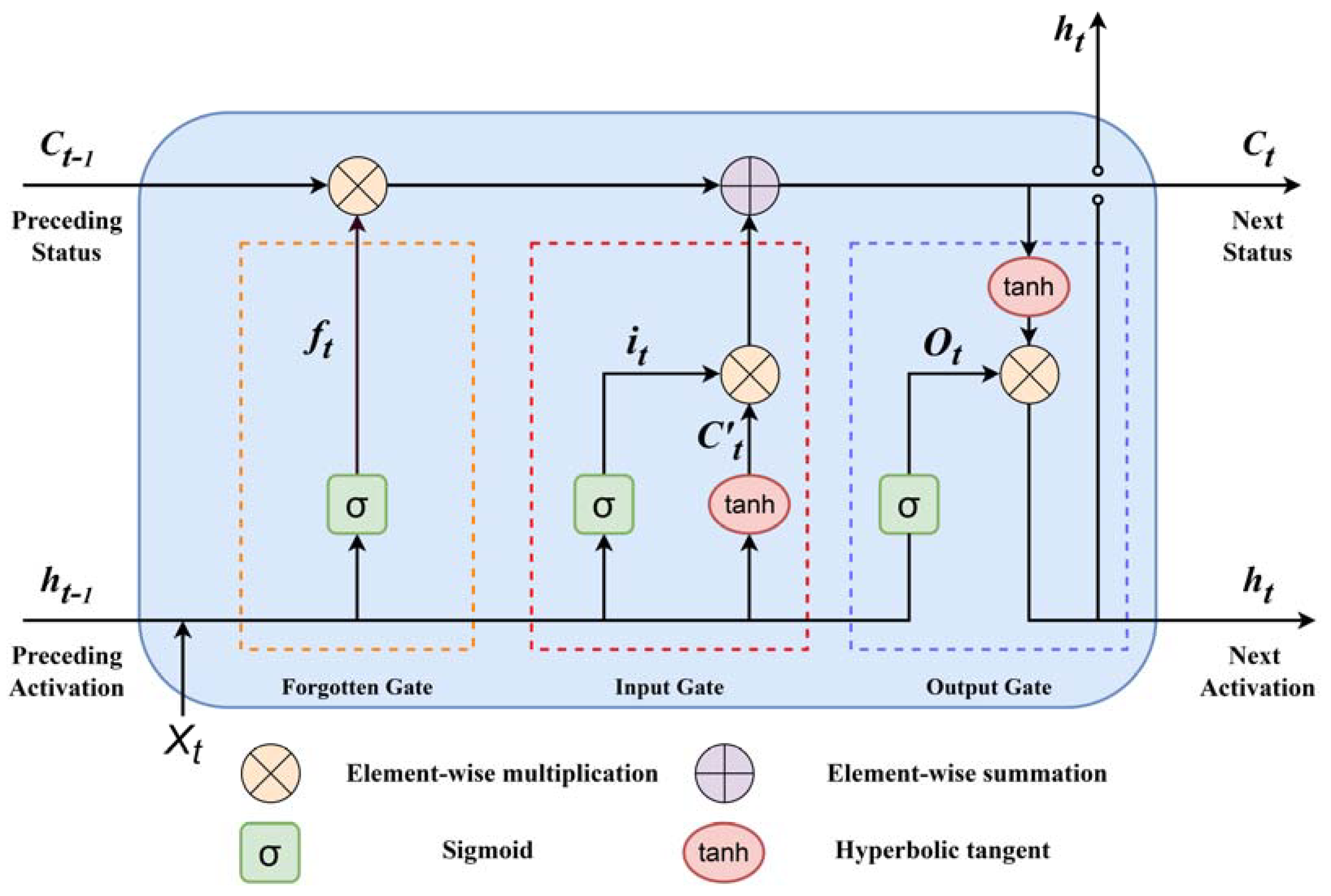
Figure 2.
The mixed VMD–EEMD–LSTM second-order decomposition model.
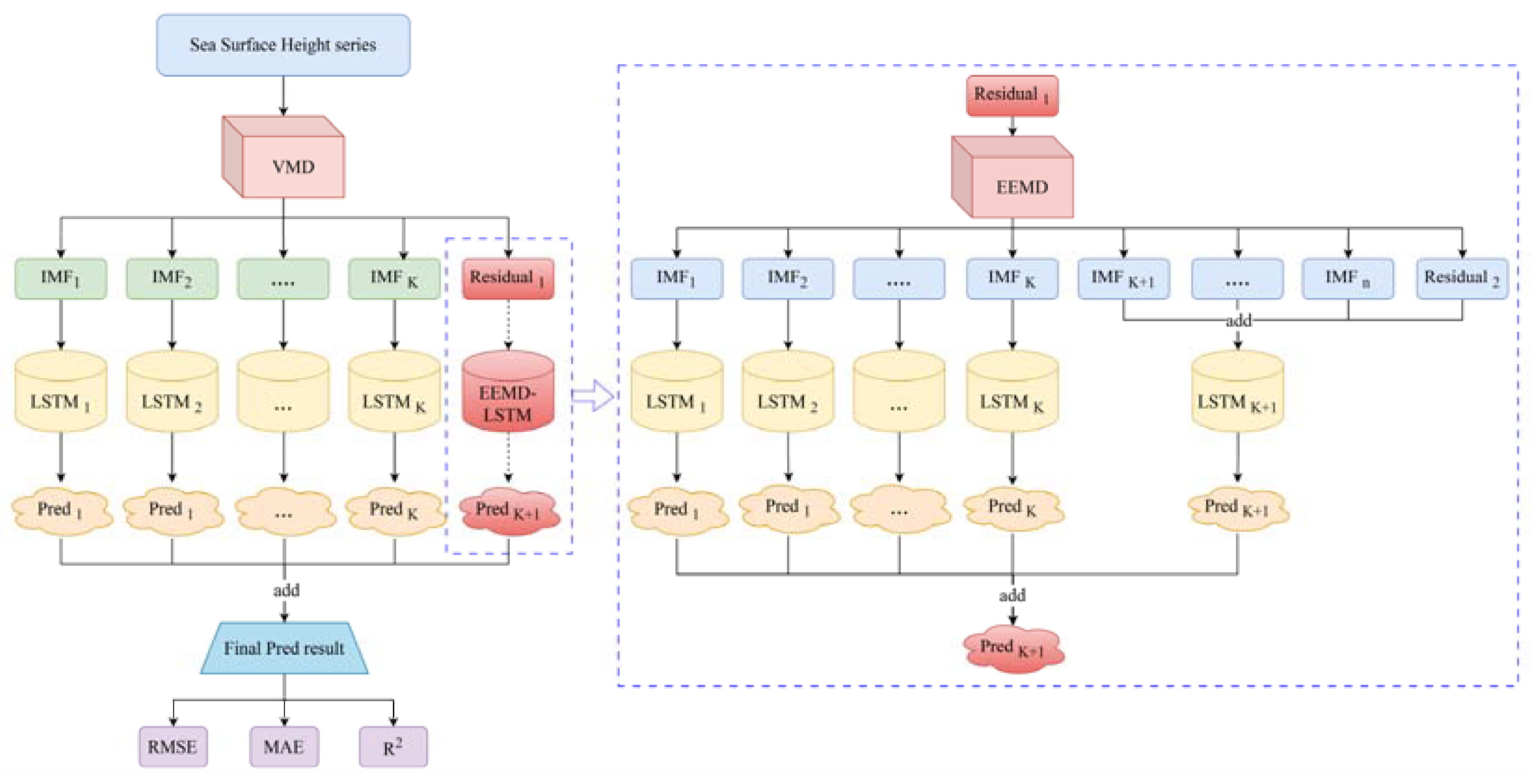
Figure 3.
Comparison of the evaluation indicators of each model at different sites
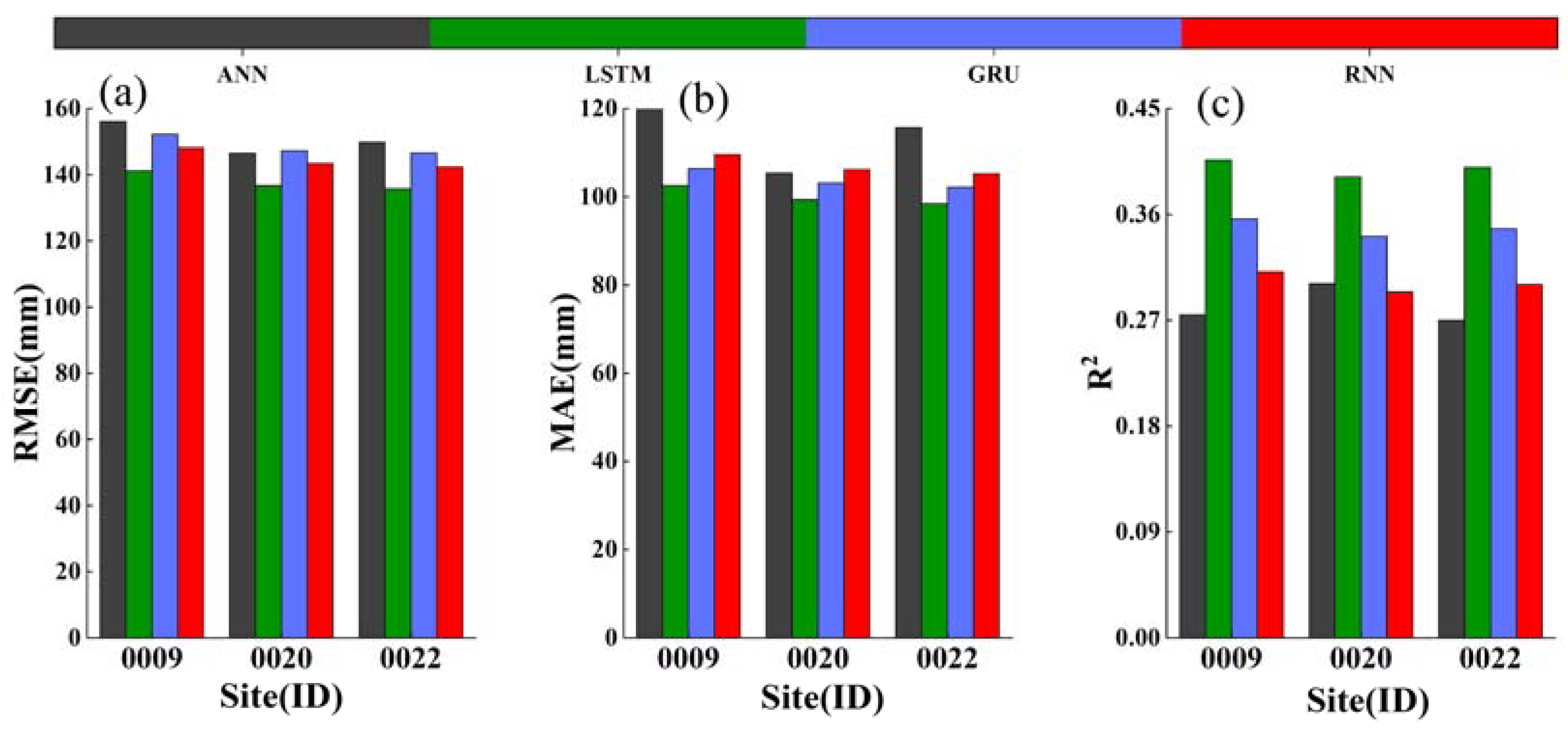
Figure 4.
Predictions of IMF and residual series under VMD (a) and EMD (b) decomposition.
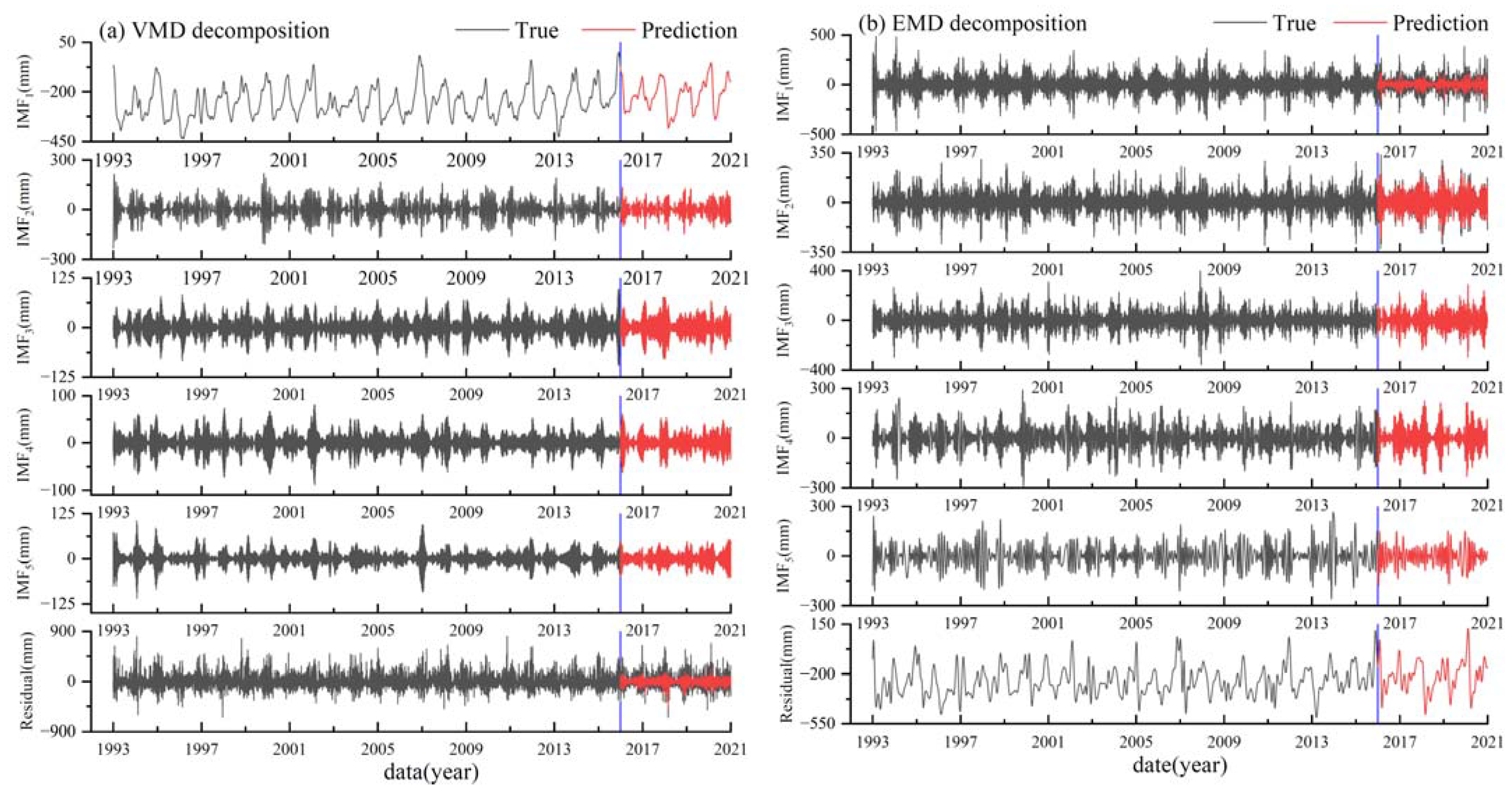
Figure 5.
Predictions of IMF and residual series under EEMD (c) and CEEMDAN (d) decomposition.
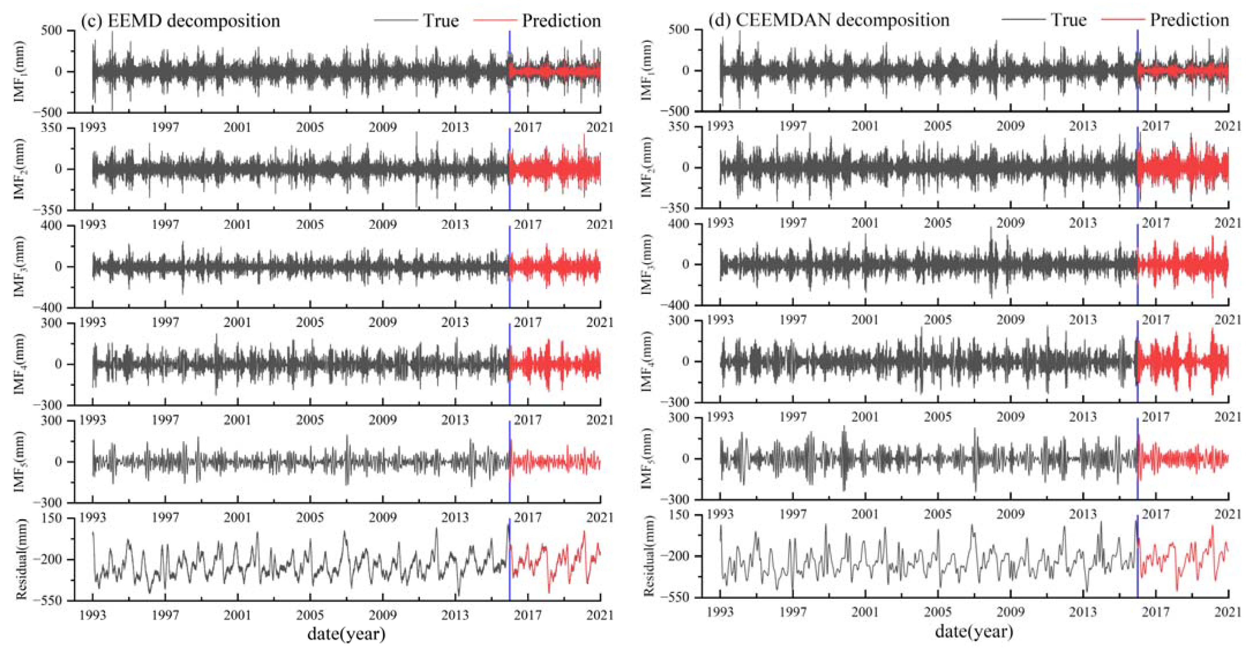
Figure 6.
Predictions and errors of each mixed model (TURE in the figure is the original time series of sea-level high. (a) represents the prediction results for the mixed models at the Maassluis station sea-level high; and (b) represents the prediction error R by the mixed models at the Maassluis station sea-level high.)
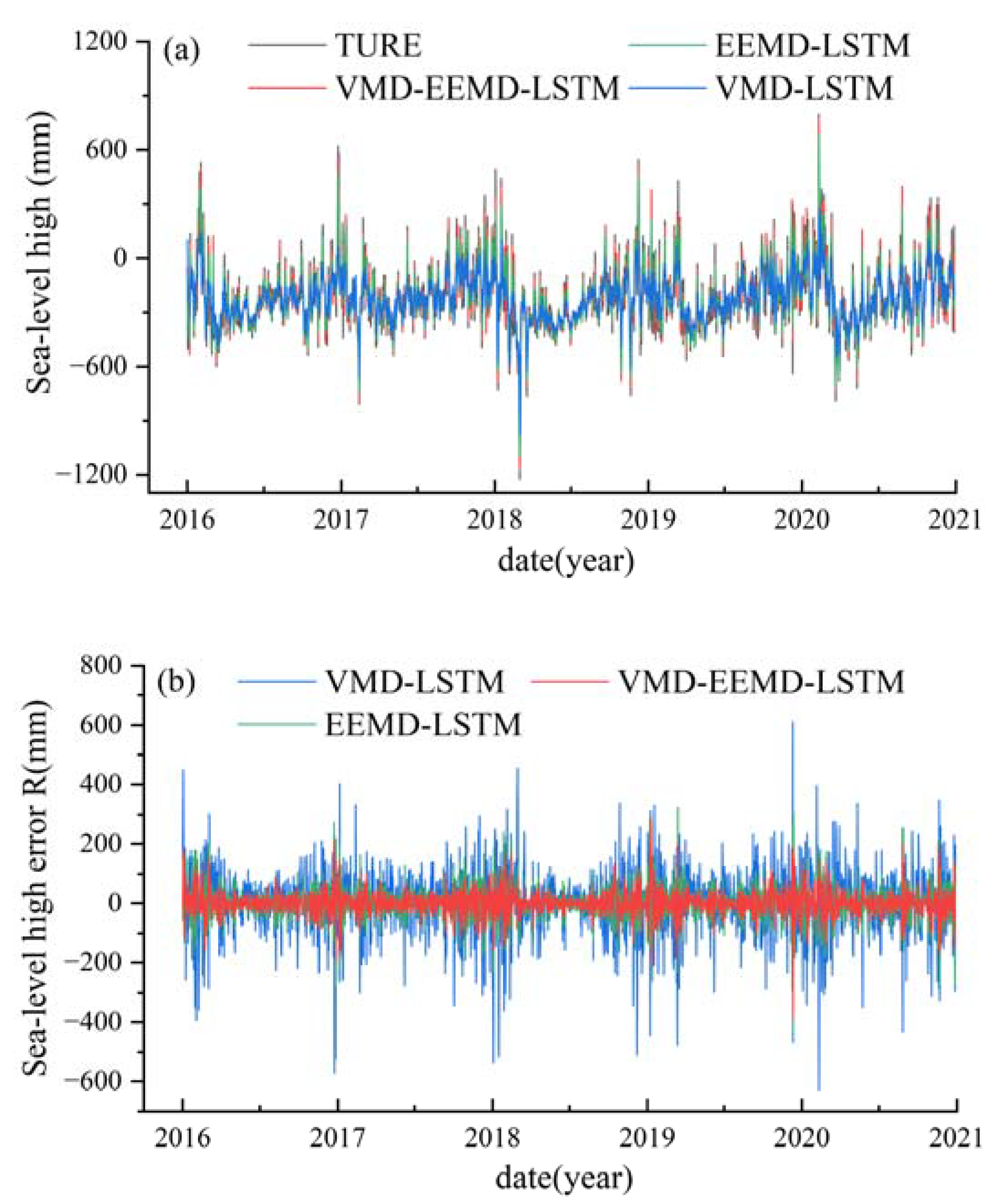
Figure 7.
Accuracy evaluation indexes of the predictions of each mixed model (The units for RMSE and MAE are both (mm).
Figure 7.
Accuracy evaluation indexes of the predictions of each mixed model (The units for RMSE and MAE are both (mm).
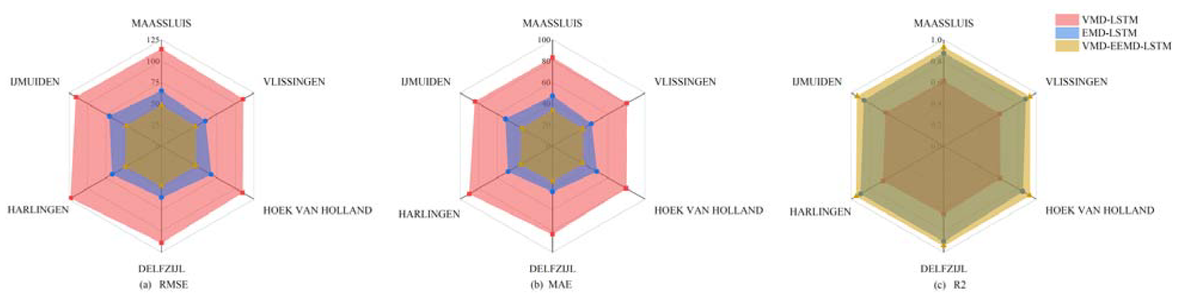

Table 1.
Details the of satellite altimetry data.
| Site | ID | Longitude (°) | Latitude (°) | Time span(years) |
|---|---|---|---|---|
| Maassluis | 0009 | 4.25 | 51.92 | 1993–2020 |
| Vlissingen | 0020 | 3.60 | 51.44 | 1993–2020 |
| Hoek Van Holland | 0022 | 4.12 | 51.98 | 1993–2020 |
| Delfzijl | 0023 | 4.75 | 52.96 | 1993–2020 |
| Harlingen | 0025 | 5.41 | 53.18 | 1993–2020 |
| Ijmuiden | 0032 | 4.56 | 52.46 | 1993–2020 |
Table 2.
Prediction accuracy of VMD-LSTM model under different K-value decomposition. (VMDK-LSTM (K=3,4,5,6,7,) is a prediction model obtained by VMD decomposition under this K value.)
Table 2.
Prediction accuracy of VMD-LSTM model under different K-value decomposition. (VMDK-LSTM (K=3,4,5,6,7,) is a prediction model obtained by VMD decomposition under this K value.)
| Model | Series | RMSE (mm) | MAE (mm) | R2 | Model | Series | RMSE (mm) | MAE (mm) | R2 |
|---|---|---|---|---|---|---|---|---|---|
| VMD3-LSTM | IMF1 | 0.48 | 0.37 | 1.00 | VMD6-LSTM | IMF1 | 0.44 | 0.34 | 1.00 |
| IMF2 | 0.87 | 0.64 | 1.00 | IMF2 | 0.56 | 0.42 | 1.00 | ||
| IMF3 | 1.26 | 0.95 | 1.00 | IMF3 | 0.77 | 0.56 | 1.00 | ||
| Residual | 125.61 | 91.01 | 0.29 | IMF4 | 1.74 | 1.31 | 1.00 | ||
| ALL | 125.42 | 90.84 | 0.53 | IMF5 | 1.15 | 0.87 | 1.00 | ||
| VMD4-LSTM | IMF1 | 0.48 | 0.36 | 1.00 | IMF6 | 0.67 | 0.51 | 1.00 | |
| IMF2 | 0.59 | 0.45 | 1.00 | Residual | 115.09 | 85.26 | 0.16 | ||
| IMF3 | 1.72 | 1.30 | 0.99 | ALL | 114.95 | 85.12 | 0.61 | ||
| IMF4 | 1.03 | 0.78 | 1.00 | VMD7-LSTM | IMF1 | 0.46 | 0.35 | 1.00 | |
| Residual | 118.53 | 86.06 | 0.22 | IMF2 | 0.57 | 0.43 | 1.00 | ||
| ALL | 118.30 | 85.81 | 0.58 | IMF3 | 0.57 | 0.43 | 1.00 | ||
| VMD5-LSTM | IMF1 | 0.46 | 0.35 | 1 | IMF4 | 0.74 | 0.55 | 1.00 | |
| IMF2 | 0.55 | 0.41 | 1 | IMF5 | 1.67 | 1.27 | 0.99 | ||
| IMF3 | 0.81 | 0.59 | 1 | IMF6 | 0.96 | 0.72 | 1.00 | ||
| IMF4 | 1.58 | 1.21 | 0.99 | IMF7 | 0.56 | 0.42 | 1.00 | ||
| IMF5 | 0.69 | 0.53 | 1 | Residual | 111.77 | 83.78 | 0.03 | ||
| Residual | 114.71 | 83.48 | 0.21 | ALL | 114.81 | 86.10 | 0.61 | ||
| ALL | 114.33 | 83.11 | 0.61 | ||||||
Table 3.
Hyperparameter settings for each model.
| Model | ANN | RNN | GRU | LSTM | Instructions |
|---|---|---|---|---|---|
| Training set | 7305 | 7305 | 7305 | 7305 | Training data for model training (1993–2012) |
| Validation set | 1095 | 1095 | 1095 | 1095 | Validation data for tuning the hyperparameters and preventing overfitting (2012–2015) |
| Test set | 1827 | 1827 | 1827 | 1827 | Testing data for evaluating the model’s performance (2015–2020) |
| Epochs | 50 | 50 | 50 | 50 | Number of iterations of the model |
| Learning rate | 0.001 | 0.001 | 0.001 | 0.001 | Hyperparameter controlling the step size of the updates of the model’s parameters |
| Input_size | 1 | 1 | 1 | 1 | Dimensionality of the input layer |
| Output_size | 1 | 1 | 1 | 1 | Dimensionality of the output layer |
| Hidden_size | 256 | 256 | 256 | 256 | Dimensionality of the hidden layer |
| Seq_len | 12 | 12 | 12 | 12 | Length of each sliding data window |
| Batch_size | 16 | 16 | 16 | 16 | Batch size for one-time input in the time series data |
Table 4.
Summary of each evaluation index of the accuracy of the time series predictions of different decomposition methods.
Table 4.
Summary of each evaluation index of the accuracy of the time series predictions of different decomposition methods.
| Model | Series | RMSE (mm) | MAE (mm) | R2 |
|---|---|---|---|---|
| VMD-LSTM | IMF1 | 0.46 | 0.35 | 1.00 |
| IMF2 | 0.55 | 0.41 | 1.00 | |
| IMF3 | 0.81 | 0.59 | 1.00 | |
| IMF4 | 1.58 | 1.21 | 0.99 | |
| IMF5 | 0.69 | 0.53 | 1.00 | |
| Residual | 114.71 | 83.48 | 0.21 | |
| ALL | 114.33 | 83.11 | 0.61 | |
| EMD-LSTM | IMF1 | 76.58 | 58.36 | 0.19 |
| IMF2 | 34.27 | 23.51 | 0.80 | |
| IMF3 | 7.31 | 4.82 | 0.99 | |
| IMF4 | 1.06 | 0.59 | 1.00 | |
| IMF5 | 0.44 | 0.30 | 1.00 | |
| Residual | 0.80 | 0.46 | 1.00 | |
| ALL | 82.43 | 61.38 | 0.80 | |
| EEMD-LSTM | IMF1 | 63.03 | 45.98 | 0.34 |
| IMF2 | 17.58 | 11.94 | 0.90 | |
| IMF3 | 2.67 | 1.85 | 1.00 | |
| IMF4 | 0.50 | 0.32 | 1.00 | |
| IMF5 | 0.29 | 0.22 | 1.00 | |
| Residual | 12.24 | 9.68 | 0.98 | |
| ALL | 65.00 | 47.21 | 0.87 | |
| CEEMDAM-LSTM | IMF1 | 76.94 | 58.05 | 0.19 |
| IMF2 | 33.51 | 23.11 | 0.80 | |
| IMF3 | 6.90 | 4.54 | 0.99 | |
| IMF4 | 1.11 | 0.69 | 1.00 | |
| IMF5 | 0.37 | 0.28 | 1.00 | |
| Residual | 0.44 | 0.34 | 1.00 | |
| ALL | 82.82 | 61.16 | 0.80 |
Table 5.
Improvement ratio of the accuracy of the predictions by the VMD–EEMD–LSTM model (the VMD–LSTM column in the table represents the degree of improvement achieved by the VMD–EEMD–LSTM model compared with the VMD–LSTM model according to the three evaluation indices, and likewise for the EEMD–LSTM column).
| Site | VMD–LSTM | EEMD–LSTM | ||||
| IRMSE (%) | IMAE (%) | (%) | IRMSE (%) | IMAE (%) | (%) | |
| Maassluis | 58.19 | 59.62 | -52.49 | 26.46 | 28.91 | -6.60 |
| Vlissingen | 58.29 | 59.28 | -54.04 | 22.52 | 22.18 | -5.17 |
| Hoek Van Holland | 57.69 | 59.05 | -52.45 | 30.97 | 32.00 | -8.98 |
| Delfzijl | 58.85 | 60.04 | -46.64 | 22.61 | 22.81 | -4.54 |
| Harlingen | 60.52 | 61.79 | -44.20 | 27.12 | 28.28 | -5.26 |
| Ijmuiden | 58.56 | 59.95 | -49.26 | 31.99 | 33.81 | -8.64 |
Disclaimer/Publisher’s Note: The statements, opinions and data contained in all publications are solely those of the individual author(s) and contributor(s) and not of MDPI and/or the editor(s). MDPI and/or the editor(s) disclaim responsibility for any injury to people or property resulting from any ideas, methods, instructions or products referred to in the content. |
© 2023 by the authors. Licensee MDPI, Basel, Switzerland. This article is an open access article distributed under the terms and conditions of the Creative Commons Attribution (CC BY) license (http://creativecommons.org/licenses/by/4.0/).
Copyright: This open access article is published under a Creative Commons CC BY 4.0 license, which permit the free download, distribution, and reuse, provided that the author and preprint are cited in any reuse.


