
Submitted:
20 October 2023
Posted:
23 October 2023
You are already at the latest version
Abstract
Accurate prediction of the degree of airport delays under the influence of convective weather is crucial for collaborative traffic management implementation and improving the efficiency of airport operations. However, existing studies usually only consider numerical-type quantitative features of weather-affected traffic in their models, and lack the introduction of spatial information to comprehensively portray the traffic operation scenarios under the influence of weather. In order to overcome this problem, this paper firstly designs a new image representation of weather-affected air traffic, and constructs a multi-channel traffic and weather scene image (MTWSI) by populating the airspace two-dimensional grid with traffic and meteorological information to represent the overall traffic operation situation in the terminal area under the influence of convective weather; then, a deep convolutional neural network-based airport delay prediction model ( ADLCNN), which takes MTWSI images as input and uses a specific CNN model to extract the deep features that affect traffic operation in it to input into the subsequent classification algorithm to predict the flight delay level; finally, a series of comparative experiments are carried out on the operational data of Guangzhou Baiyun Airport, and the experimental validation shows that, compared with the traditional machine learning methods, the proposed CNN-based airport delay prediction The experimental validation shows that the proposed CNN-based airport delay prediction model has satisfactory prediction performance compared with the traditional machine learning methods, which also proves that the proposed MTWSI method can more comprehensively respond to the real traffic conditions.
Keywords:
airport delay prediction
; convective weather
; image recognition
; deep convolutional neural network
; taxonomic imbalance
0. Introduction
Airport delay is an evaluation indicator of the overall operational performance of an airport, reflecting its operational efficiency and the rationality of flight scheduling. The interaction of weather factors, air traffic control, aircraft maintenance, flight scheduling, airport facilities and human factors is the main reason for exacerbating airport delays. Severe airport delays often cause flight congestion and chaos, increase the risk of flight conflicts and accidents, and adversely affect flight safety while causing great inconvenience to airlines, passengers and airports. To mitigate the negative impacts of delays, intelligent airport delay prediction systems have emerged and become the key to Intelligent Air Traffic Management (IATM). The goal of IATM is to improve the efficiency and quality of airport operations and achieve a higher level of airport management by providing real-time monitoring and early warning of delays of airport flights in the coming period of time through Artificial Intelligence (AI) technology.
The impact of weather factors on airport delays is very significant, especially terminal area convective weather, such as high winds that can affect aircraft landing and take-off, hailstorms that can affect aircraft casings and engines, and thunderstorms that can affect the normal operation of ground-based equipment, which can lead to flight delays. Therefore, for the impact of terminal area convective weather on airport delays, an intelligent airport delay prediction system needs to consider weather factors. Thus, the research objective of this paper is to characterise the impact of terminal area convective weather on flight operations by using a multi-channel pictorial approach - accurately portraying the relative positional distributions of terminal area convective weather and inbound and outbound flight flows - and thus improve the existing delay prediction models to enhance prediction accuracy and practicality.
Compared with existing studies, the contributions of this study are mainly: to propose a new data representation method, i.e. multi-channel traffic and meteorological scene images, to rasterise convective weather and inbound and outbound flight data in the terminal area, and merge them into a multi-channel image to represent the air traffic operation scenarios under the influence of convective weather; and to use deep convolutional neural networks to fully mine the hidden delay impact information in the multi-channel images and learn a high-precision airport delay prediction model.
The main organisational framework of this paper is as follows: chapter 2 summarises the relevant literature on flight delay prediction. Chapter 3 describes the classification method of airport delay class. Chapter 4 details a deep metric learning based model for airport delay class prediction. Chapter 5 details the dataset we use and validates the superiority of the proposed model through comparative experiments. Chapter 6 summarises the full paper and suggests future research directions.
1. Related Work
The study of airport delays in relation to severe weather has been one of the more cutting-edge and critical areas of research for many years, since the late 1990s, with organisations such as MITRE, MIT Lincoln Laboratory and NASA leading the way in this area. The field is dominated by research centred around the Weather Impacted Index (WITI) developed by MITRE, as well as MITRE’s Flow Contingency Management (FCM) research, the application of Ensemble Weather Forecasts for weather forecasting, and the development of a new weather forecasting system. Weather Forecasts (EWF) to quantify weather uncertainty, and the FAA-led Air Traffic Management-Weather Integration (ATM-Weather Integration) study.
In terms of WITI, a great deal of research has been done by scholars at home and abroad. Callaham et al [1] developed the WITI concept in 2001 with the aim of quantifying the impact of unfavourable weather on the operation of the National Airspace System (NAS), which is particularly applicable to the assessment of weather in large-scale and long-duration scenarios. The concept is mainly used to assess the impact of weather on air traffic. Sridhar and Chatterji et al [2,3,4,5] constructed various models to assess the daily delays in the national airspace through regression methods between 2005 and 2007, taking into account the effects of weather, flight traffic, airport size, etc., which provided a deeper study of the relationship between airport delays and factors such as weather powerful tools and methods. Klein et al [6,7] proposed the concepts of en route weather impact air traffic index E-WITI, terminal area weather impact traffic index T-WITI and queuing delays in 2007, and introduced the application of predictive weather impact traffic index WITI-FA, which provided a new way of thinking for the development of airport delay prediction systems. Klein et al [8,9] proposed a method for quantitative assessment of sector availability under the influence of weather based on a scanline algorithm that incorporates the WITI-FA index for operational assessment of a wide range of convective weather forecast products between 2008 and 2009.Cook et al [10] quantified the impact of weather factors on air traffic using the Weather Impact Traffic Index (WITI) in 2009. By calculating the adverse effects of seven weather factors, it was found that low visibility, convective weather and wind had the most significant impact on air traffic. Mukherjee et al [11] in 2013 used the WITI to classify the number of weather days and analysed the differences between weather conditions for rerouting and route planning as prescribed by the National Prediction Manual (NPM). Their study aimed to assess the effectiveness of the National Advance Planning Manual (NAPM) for air traffic planning under the influence of weather and provided recommendations. Guo Ye Chenfeng et al [12] proposed a simplified airport-oriented WITI and verified its feasibility for airport delay prediction.
Most of the above studies use numerical impacts to quantify the impact of convective weather on traffic operation, focusing on the quantification of the overall impact of the terminal area, and do not take into account the spatial distribution of convective weather in the terminal area and its relative position to the flight trajectory, which can not comprehensively and objectively reflect the actual impacts of convective weather on flight operation in the terminal area, resulting in the delay prediction model is not very accurate, and it is difficult to form an effective aid to decision-making for airport Therefore, this paper proposes a method for predicting airport delay level based on deep metric learning. The method takes the airport delay grade as the research object, and first uses the FCM algorithm to cluster the airport delay-related features, extract the airport delay grade classification rules, and obtain the delay grade labels. Then, the actual collected weather avoidance area (WAF) and radar track (ADS-B) data of the terminal area are rasterised to generate multi-channel image features containing spatial location information. After that, the airport delay level prediction model is constructed based on deep convolutional neural network. The aim of the proposed airport delay level prediction method is to construct a comprehensive and objective characterisation and monitoring of the overall operation posture of the terminal area by accurately predicting the overall delay condition of the airport during convective weather, in order to support the traffic management decision in the pre-tactical phase and to improve the operation efficiency of the terminal area.
2. Classification of airport departure delays
2.1. Airport delay indicator selection
Airport delay level is an overall description of all kinds of delays at an airport during a certain period of time, which is an important criterion for measuring the efficiency of airport operation. Selecting a single feature for description can only judge the delay level from one aspect of the delay result, and cannot fully reflect the flight delay situation and the delay evolution law. Therefore, in this paper, the average delay time of departure flights and the on-time rate of departure flights are selected to evaluate the airport departure delay level from the perspectives of the degree of delay and the reliability of flights.
2.2. Classification method
Airport delay classification can be regarded as an unsupervised learning problem, so in this paper, we will use the fuzzy C-mean (FCM) clustering method for the classification. The FCM algorithm is a fuzzy mathematics-based clustering method, which is better suited for certain fuzzy clustering problems because of its ability to assign multiple categories of belonging to each sample compared to traditional hard clustering methods.
The FCM algorithm works as follows: Let the given data set be , we need to find a number c that divides the dataset into c classes , then the affiliation matrix of the dataset is , is a matrix of c rows and n columns where the element denotes the probability that the element belongs to the class, .
We specify as the clustering centre of the class, and there are a total of c, and the FCM algorithm satisfies the following conditions:
The principle of the FCM algorithm is to minimise the criterion function through continuous iteration.
2.3. Extraction of grading rules
After FCM cluster analysis, the flight delay dataset can be divided into different clusters, each representing a level of delay. Therefore, each cluster can be regarded as a delay level, which can be used to classify the degree of delay at the airport. Figure 1 demonstrates the trend of the contour coefficient with the number of clusters, where the number of clusters of 2 corresponds to the highest contour coefficient, indicating that the samples in the clustering results are more cohesive and separated at this time. Figure 2 demonstrates the distribution of different delay characteristics within each cluster when the number of clusters is 2, in which the distribution of average departure delays between two clusters is relatively more separated, while there is a staggered distribution of flight punctuality, but the overall flight punctuality of the samples in Cluster 0 is lower, and the overall flight punctuality of the samples in Cluster 1 is higher. Thus, we divide the airport delay class into two categories: Cluster 0 represents the general delay class, whose average departure delay is less than 50 min and flight punctuality is higher; Cluster 1 represents the severe delay class, whose average departure delay is higher than 50 min and flight punctuality is lower. The later experiments on airport delay level prediction will be viewed as dichotomous predictions.
3. Convolutional neural network-based airport delay level prediction model
Predicting airport delay levels under the influence of convective weather becomes difficult because existing numerical type features cannot accurately and comprehensively characterise the impact of convective weather on flight operations in terminal areas. Therefore, combining the advantages of deep learning, in this paper, we convert air traffic scene information into images and use deep learning techniques to extract useful information. Considering the image-based approach, we propose an end-to-end learning method for airport delay level prediction using a deep convolutional neural network learning strategy, which is named ADLCNN. Figure 3 illustrates the framework structure of the proposed ADLCCN method. Specifically, the raw weather and traffic data are firstly rasterised to construct MTWSIs, and then CNNs are used to mine useful information from the images through nonlinear transformations to achieve the feature learning process, and the learned features are used to assess the delay level of the airport.
3.1. Data description
The data used in this study include Weather Advective Flow (WAF) data and air traffic data, where the air traffic data are further divided into static airspace data and dynamic flight data. WAF data are weather information data in convective clouds detected by meteorological radar, which are used to predict and monitor extreme weather events, such as torrential rains, thunderstorms, tornadoes, and so on. Each WAF data consists of 1250×1250 data points, and each data point represents the convective weather intensity within 200m×200m. Static airspace data refers to some fixed and unchanging aeronautical airspace information, consisting of latitude and longitude data, which is used to delineate the airspace structure. Dynamic flight data refers to the flight data that is updated in real time with time changes, such as aircraft position, altitude, speed, navigation, flight status and other information, which is obtained through satellite communication or ADS-B transmission equipment. The deep learning method based on MTWSI proposed in this paper mainly uses static data to rasterise the airspace and uses some method to populate the rasterised airspace with dynamic flight data in order to generate the traffic and meteorological scenarios, and then uses the generated images for feature extraction in order to perform the task of predicting the delay level of an airport.
3.2. Multi-channel image construction
Convective weather in the terminal area is an important factor in increasing delays at airports, especially when a large number of flights are planned. At the same time, the relative position between the convective weather and the flight path determines the severity of this effect. For this reason, this paper proposes a new data representation method called multi-channel air traffic and meteorological scene images to portray the impact of convective weather within the terminal area on flight operations and to serve as an input to airport delay prediction models.
The image is composed of a two-dimensional matrix, so we need to rasterise the target terminal area first as a basis for subsequent images. To ensure the regularity of the image and the ease of subsequent image manipulation, this study uses the outer square of the terminal area as the extent of the image and divides the target terminal area into grid maps of appropriate precision. The time span of our individual traffic and weather scene samples is 1 h. In order to ensure that real traffic and weather data exists in each grid and that the accuracy of the grid is sufficiently high, we divide the terminal area into 125x125 grid maps, and the width of each grid is set to be 2 km. Since each grid contains latitude and longitude information, we can map the position of the aircraft in the airspace to the corresponding grid, which allows us to populate the grid with traffic operation information, such as traffic volume, average flight altitude, average flight speed, etc. However, since a grid can only be populated with one value and cannot contain a large amount of information at the same time, multiple 2D matrices are needed to store the traffic and weather information. These different 2D matrices can be understood as multi-channel images, which can express the traffic and meteorological information in the same scene from different perspectives. When these channels are superimposed at the same time, the real air traffic scene can be well reproduced.
The traffic scenario is a period of time rather than an instant, and the airport delay level is not an instantaneous metric, so in order to reflect the real situation of flight operations affected by convective weather over a period of time, we chose to map all the traffic and convective weather data received during this period onto a grid map. Specifically, by mapping the flight track data to the corresponding grids of the 2D grid matrix, the image will show the number of flights passing through each grid during a certain period of time as well as the overall flight status of the flights. Here, we chose to utilise the flight trajectory, altitude and speed traffic information to generate three types of images, which are referred to as the flight volume channel, the average altitude channel and the average speed channel, as shown in Figure 4.
In addition, a convective weather channel was constructed to reflect convective weather conditions within the terminal area. The original convective weather WAF data is a two-dimensional matrix consisting of 1250x1250 data points, and the dimensionality does not match with several channels related to traffic, so it needs to be dimensionally downgraded. Thus, referring to the concept of rasterised WSI, this paper correspondingly matches the convective weather WAF data to a 125×125 terminal area raster and calculates the WSI inside each raster, which makes the data dimensionality matched, and at the same time preserves the weather severity as well as the spatial distribution information. As shown in Figure 5, (a), (b), and (c) demonstrate the distribution of weak, moderate, and strong convective weather within the terminal area, respectively.
3.3. CNN Models for Predicting Airport Delay Levels
3.3.1. CNN Models for Predicting Airport Delay Levels
CNNs have powerful grid data processing capabilities and are widely used in image analysis [15]. The main structure of CNNs includes an input layer, a convolutional layer, a pooling layer, and a fully connected layer. The information in the input layer is processed through element transformation and extraction in the convolution and pooling layers. This local information in the convolution and pooling layer is further integrated by the fully connected layer and mapped to the output signal through the output layer.
The convolutional layer is the most important and unique layer in a CNN as it allows for the extraction of features of the input variables through convolutional kernels. Unlike fully connected neural networks, the convolutional layer of a CNN connects only some of the neurons of the previous layer. The size of the convolution kernel is smaller than the size of the input matrix. The convolutional layer uses convolution operations rather than the usual matrix operations to output the feature map. The formula for each element in the feature map is:
Where is the output value of the feature matrix in i row and j column; is the value of the input matrix in row and column; is the selected activation function; is the weight of the convolution kernel in m row and n column; b is the deviation of the convolution kernel. The input matrix is usually convolved using multiple kernels. Each convolution kernel will extract a feature from the input matrix and generate a feature map. Afterwards, the pooling layer reduces the length and width of the previous feature map by downsampling, which improves the computational efficiency.
3.3.2. Network structure of the ADLCNN method
The network is used to learn and predict the degree of delay at a given airport given convective weather and traffic operation information. The input data is a multi-channel input image (MTWSI) converted from traffic and meteorological data, and the conversion process can be found in Section 3.2. The output labelled data is the airport delay level obtained from FCM clustering.
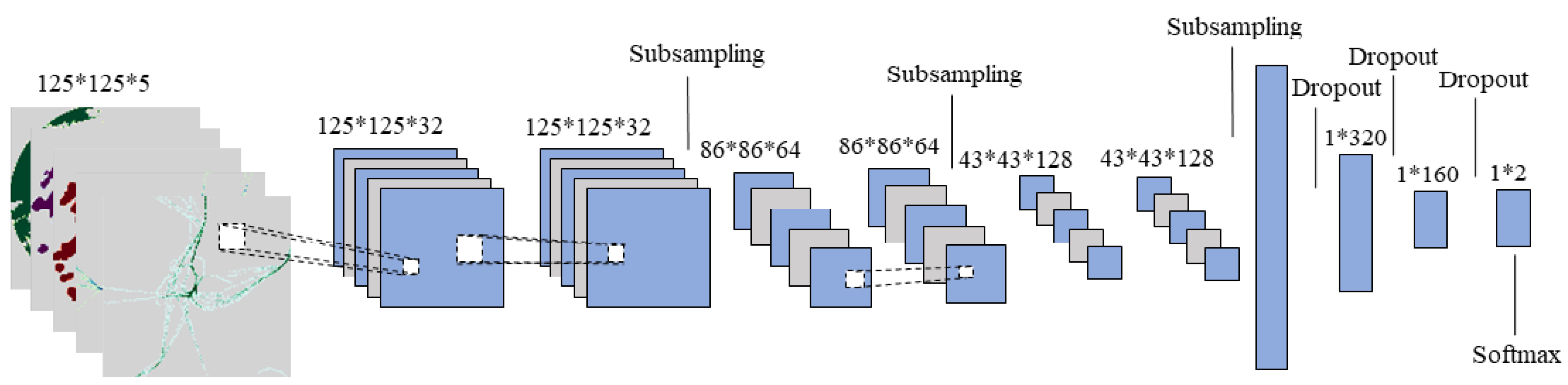
The model includes six convolutional layers, a pooling layer, and three fully connected layers. Borrowing the idea of VGG, this paper adopts a small convolutional kernel (3*3) and replaces the large convolutional kernel with multiple consecutive convolutional layers, because multiple nonlinear layers can increase the depth of the network to ensure learning of more complex patterns with lower computational cost. The number of convolution kernels in each convolutional layer is (32, 32, 64, 64, 128, 128) and the maximum pooling size is (2*2). The activation function of ReLU is used. The learning rate of the model is 0.001 and the batch size is 128.The goal of deep learning model training is to iteratively optimize the parameters of the network model and learn the distribution of the data from the training set samples. Usually, the optimization direction is determined by an objective function, which consists of an error term (J) and a regularity term (R):
In the equation, and X are Y are the inputs and outputs of the model. The loss function and regularization term are denoted by J and R respectively. denote the parameters of the deep neural network, and is the weight of the regularization term. In this paper, the cross-entropy is used as the loss function and is determined by where and are the real and actual labels of the first i training sample. The use of shedding layer effectively reduces the occurrence of overfitting, and the Adam optimizer is applied to improve the performance of the gradient descent algorithm.
Figure 6.
Network architecture of our convolutional neural network.
4. Experiments and Discussions
4.1. Experimental Configuration
In this section, experiments are conducted on real data in order to verify the effectiveness of our proposed deep metric learning-based airport delay level prediction method. The WAF and air traffic data of Guangzhou Baiyun Airport (ZGGG) in China for the whole year of 2019 are selected for the experiments, with a total of samples, and each sample corresponds to the MTWSIs generated from the one-hour WAF data and the air traffic data as well as the delay class labels provided based on the delay class classification rules in Section 2. In the following experiments, the whole dataset is divided into two parts, with 70% of the samples as the test set and the rest as the test set. In addition, two sets of comparison experiments are designed in this study, one is to compare the difference in prediction accuracy between the numerical feature processing method and the present method, and the other is to compare the effect of multi-channel images with different separate rates on prediction accuracy.
The experiments were performed on a computer with an AMD EPYC 7642 48-Core Processor, 24 GB of RAM and an NVIDIA RTX A5000 GPU. The Python programming language, version 3.7.9, was used. deep learning frameworks TensorFlow 2.4.1 and Keras 2.4.3 were used for model construction and training. Data was processed and analysed using the NumPy 1.19.5 and pandas 1.2.1 libraries. Machine learning tasks were implemented using the scikit-learn 0.24.1 library. The results were visualized using Matplotlib 3.3.4 and Seaborn 0.11.1 libraries. The experimental operating system is ubantu 20.2.
In evaluating the performance of the predictive model, this paper will use validation accuracy, precision, recall, F1 score, and Mathew’s correlation coefficient as measures.
4.2. Class Imbalance Processing
The number of samples in the original dataset for the general delay category is 4918, while the number of samples for the severe delay category is only 409, which is highly unbalanced and significantly affects the performance of the classifier. To overcome this problem, this study will use a sampling technique to improve the category distribution and avoid overlap.
Currently, sampling techniques include undersampling, oversampling and hybrid methods. Currently, the more popular and widely used are, Under-Sampling Technique (US): Random Under-Sampling (RUS), Edited Nearest Neighbours (ENN), and Tomek Links (Tomek), Oversampling Technique (OS): Random Over-Sampling (ROS), Synthetic Minority Over Sampling Technique (SMOTE), and Adaptive Synthetic (ADASYN), Combination of Under-Sampling and Oversampling (UOS): SMOTETomek & SMOTEENN. Figure 7 illustrates the original training dataset and the sampled training dataset generated by various sampling techniques to generate the sampled training dataset. The sampled data is used to train the estimation method and the original test set is used to validate the performance.
4.3. Performance comparison of delay prediction methods
The first experiment focuses on going to compare the prediction performance of the CNN-type we learnt from MTWSI with several machine learning methods based on numerical features. These machine learning methods used for comparison include Gaussian Plain Bayes (GNB), k-Nearest Neighbours (KNN), logistic Linear Regression (LLR), Support Vector Machines (SVMs), Multi-Layer Perception (MLP) and integrated learning algorithms such as Random Forests (RF) and Adaptive Boosting (AdaBoost). Table 1 summarises the prediction results for the three sampling techniques with the best prediction performance under under-sampling, over-sampling, and hybrid methods. An in-depth analysis of the table shows that the ADLCNN method proposed in this paper outperforms other traditional machine learning methods overall, regardless of the sampling technique used. In particular, the prediction performance of the ADLCNN is more balanced when using the ROS sampling technique, where the recall is 0.83 for average delays and 0.78 for severe delays, with an overall accuracy of up to 0.831.
4.4. Performance comparison of multi-channel images with different resolutions
The second experiment focuses on comparing the performance differences between ADLCNN models obtained by training with multi-channel images of different resolutions. Here, we mainly designed three different resolutions, namely 5x5, 25x25, and 125x125. In addition, this comparison experiment uses the ROS technique which makes the prediction performance of ADLCNN more balanced. Table 2 shows the prediction results of ADLCNN method under different resolutions of multi-channel images, from which it can be seen that when the resolution of multi-channel images is higher the prediction performance of ADLCNN method will be better.
5. Conclusion
Deep learning techniques are widely used in the field of image processing and have yielded fruitful results because of its powerful ability to represent complex features than other methods. However, there is limited research in airport delay prediction. Extracting more complex features by deep learning methods will improve the performance of delay prediction.
In this paper, we propose a multi-channel image-based airport delay level prediction method that can automatically extract complex weather-affected traffic operation features to learn airport delay patterns. The method mainly consists of three parts, the first part is first based on the FCM clustering algorithm to classify the airport departure delay level in a simple way; the second part is to rasterise the WAF with the incoming and outgoing flight data, and construct a multi-channel image for portraying the air traffic operation scenario under the influence of convective weather; the second part is to use the deep learning technology to learn, based on the constructed multi-channel image, the influencing airport delay information to achieve the prediction of airport delay level. Experimental results show that the proposed method is proved to have high prediction accuracy compared with traditional machine learning methods.
In the future, our method can be further improved in the following directions: (1) attempts can be made to design more complex and effective networks to further improve the model prediction performance; (2) for the airport delay classification problem, the use of clustering methods is limited in terms of explanatory power, and it needs to be further combined with domain knowledge and professional experience (3) airport delays have a strong temporal correlation, and in the future, better methods need to be used to capture the time-dependent feature information in air traffic scenarios.
Author Contributions
Conceptualization, L.Y.; methodology, L.Y., J.J. and H.C.; software, L.Z.; formal analysis, J.J. and L.Z.; investigation, L.Y. and J.J.; resources, L.Z. and J.J.; data curation, J.J.; writing—original draft preparation, L.Y. and J.J.; writing—review and editing, L.Y., J.J. and Y.Z.; supervision, H.C. and Y.Z.; project administration, H.C.; funding acquisition, L.Y. All authors have read and agreed to the published version of the manuscript.
Funding
This paper is supported by Postgraduate Research & Practice Innovation Program of NUAA(xcxjh20221618).
Acknowledgments
We would like to thank the State Key Laboratory of Air Traffic Management System of Nanjing University of Aeronautics and Astronautics for providing the data used in the model tests described in this paper.
Sample Availability
Samples of the compounds ... are available from the authors.
References
- Callaham, M.; DeArmon, J.; Cooper, A.; Goodfriend, J.; Moch-Mooney, D.; Solomos, G. Assessing NAS performance: Normalizing for the effects of weather. In 4th USA/Europe Air Traffic Management R&D Symposium, Santa Fe, New Mexico, USA, 04-07 December 2001.
- Sridhar, B.; Swei, S. Relationship between weather, traffic and delay based on empirical methods. In 6th AIAA aviation technology, integration and operations conference (ATIO), Wichita, Kansas, USA, 25-27 September 2006. [CrossRef]
- Sridhar, B.; Swei, S.; Pacific Grove; C.A. Computation of aggregate delay using center-based weather impacted traffic index. In Proceedings of the 7th AIAA Aviation Technology, Integration, and Operations Conference, Belfast, Northern Ireland, 18-20 September 2007.
- Sridhar, B.; Chen, N.Y. Short-term national airspace system delay prediction using weather impacted traffic index. Journal of guidance, control, and dynamics 2009, 32, 657-662. [CrossRef]
- Chatterji, G.; Sridhar, B. National airspace system delay estimation using weather weighted traffic counts. In AIAA Guidance, Navigation, and Control Conference and Exhibit, San Francisco, California, USA, 15-18 August 2005. [CrossRef]
- Klein, A.; Jehlen, R.; Liang, D. Weather index with queuing component for national airspace system performance assessment. In 7th FAA/Eurocontrol ATM Seminar, Barcelona, Spain, 02-05 July 2007.
- Klein, A.; Kavoussi, S.; Hickman, D.; Simenauer, D.; Phaneuf, M.; MacPhail, T. (2007, April). Using a Convective Weather Forecast Product to Predict Weather Impact on Air Traffic: Methodology and Comparison with Actual Data. In 2007 Integrated Communications, Navigation and Surveillance Conference, Herndon, Virginia, USA, 01-03 May 2007. [CrossRef]
- Klein, A.; Cook, L.; Wood, B. Airspace availability estimation for traffic flow management using the scanning method. In 2008 IEEE/AIAA 27th Digital Avionics Systems Conference, St. Paul, Minnesota, USA, 26-30 October 2008. [CrossRef]
- Klein, A.; MacPhail, T.; Kavoussi, S.; Hickman, D.; Phaneuf, M.; Lee, R. S.; Simenauer, D. NAS weather index: Quantifying impact of actual and forecast en-route and surface weather on air traffic. In 89th AMS Annual Meeting, Phoenix, Arizona, USA, 11-15 January 2009.
- Cook, L.; Wood, B.; Klein, A.; Lee, R.; Memarzadeh, B. Analyzing the share of individual weather factors affecting NAS performance using the weather impacted traffic index. In 9th AIAA Aviation Technology, Integration, and Operations Conference (ATIO) and Aircraft Noise and Emissions Reduction Symposium (ANERS), Hilton Head, South Carolina, USA, 21-23 September 2009. [CrossRef]
- Mukherjee, A.; Grabbe, S. R.; Sridhar, B. Classification of days using weather impacted traffic in the national airspace system. In 2013 Aviation Technology, Integration, and Operations Conference, Los Angeles, CA, USA, 12-14 August 2013. [CrossRef]
- Guo, Y.C.; Li, J.; Hu, M.H. An airport delay prediction method based on simplified WITI metrics. Transportation Systems Engineering and Information 2017, 17(05), 207–213.
- Zhang X. Research on similar scene identification method for air traffic control operation. Master’s Thesis (M.A.), Nanjing University of Aeronautics and Astronautics, Nanjing, China, 2021.
- Yan, R.; Liao, J.; Yang, J.; Sun, W.; Nong, M.; Li, F. Multi-hour and multi-site air quality index forecasting in Beijing using CNN, LSTM, CNN-LSTM, and spatiotemporal clustering. Expert Systems with Applications 2021, 169, 114513. [CrossRef]
- Khan, W.A.; Ma, H.L.; Chung, S.H.; Wen, X. Hierarchical integrated machine learning model for predicting flight departure delays and duration in series. Transportation Research Part C: Emerging Technologies 2021, 129, 103225. [CrossRef]
Figure 1.
Trends in number of clusters and contour coefficients.
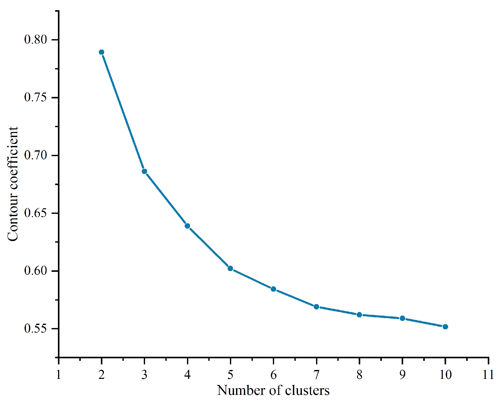
Figure 2.
Distribution of delay characteristics within different clusters.
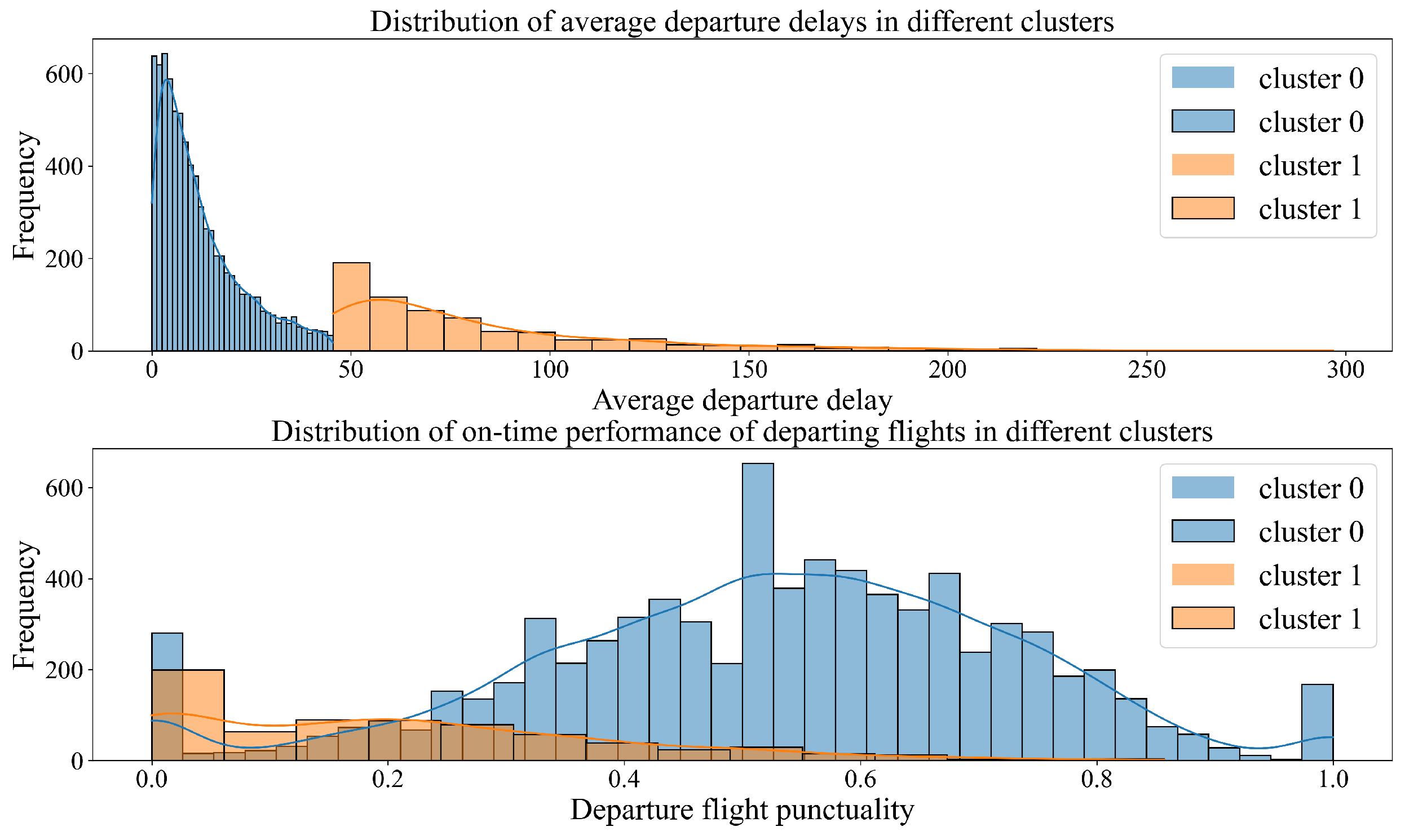
Figure 3.
Framework structure of the ADLCNN method.
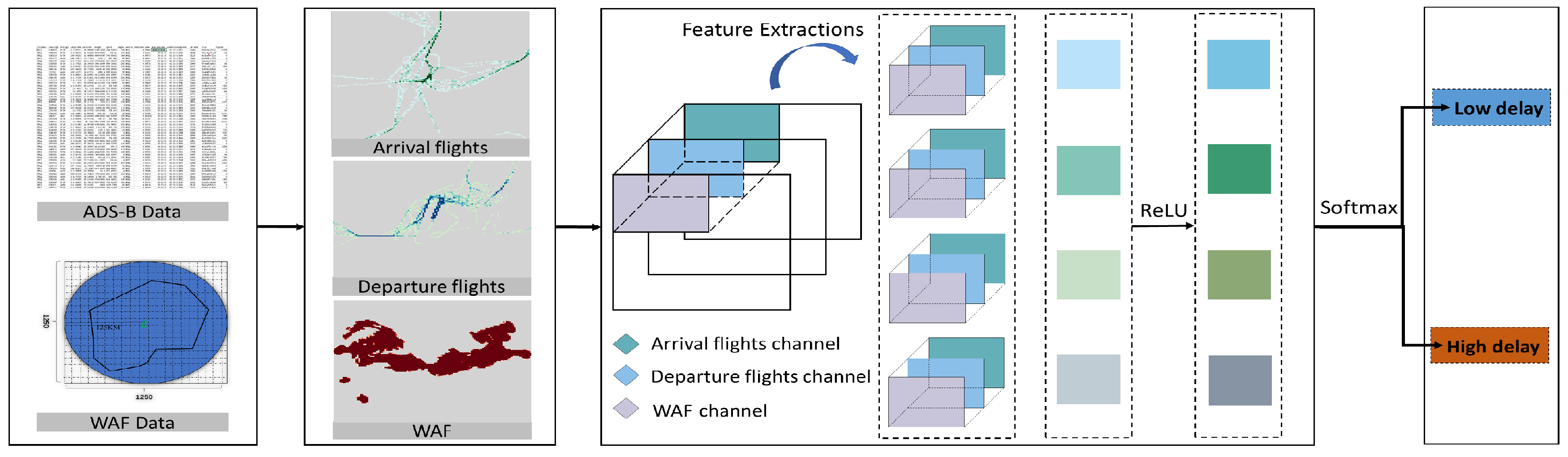
Figure 4.
(a) Flight volume channel. (b) Flight altitude channel. (c) Flight Speed channel.
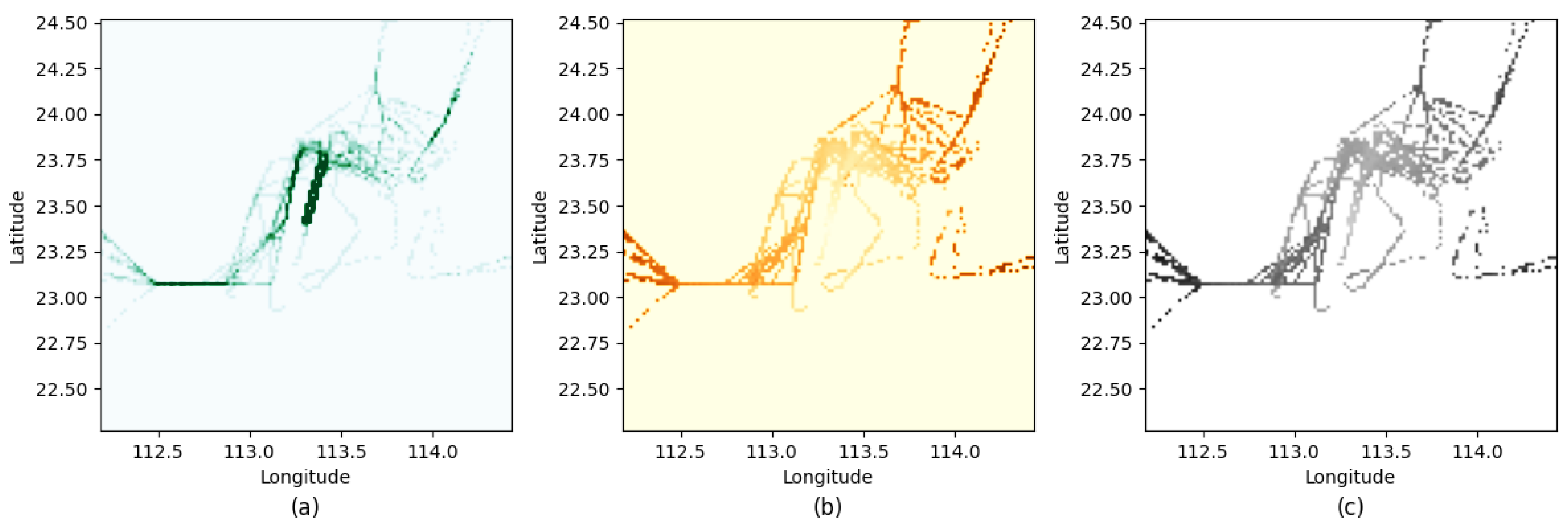
Figure 5.
(a) Weak convective weather channel. (b) Moderate convective weather channel. (c) Severe convective weather channel.
Figure 5.
(a) Weak convective weather channel. (b) Moderate convective weather channel. (c) Severe convective weather channel.
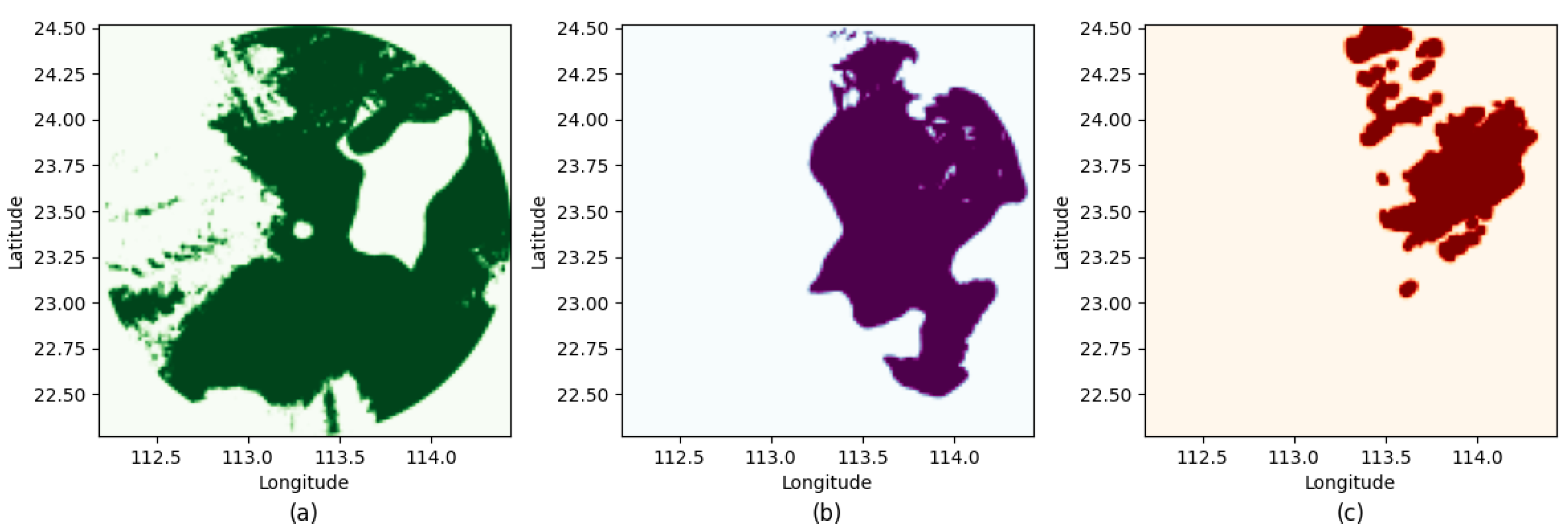
Figure 7.
Class distribution of the training set after applying various sampling techniques.
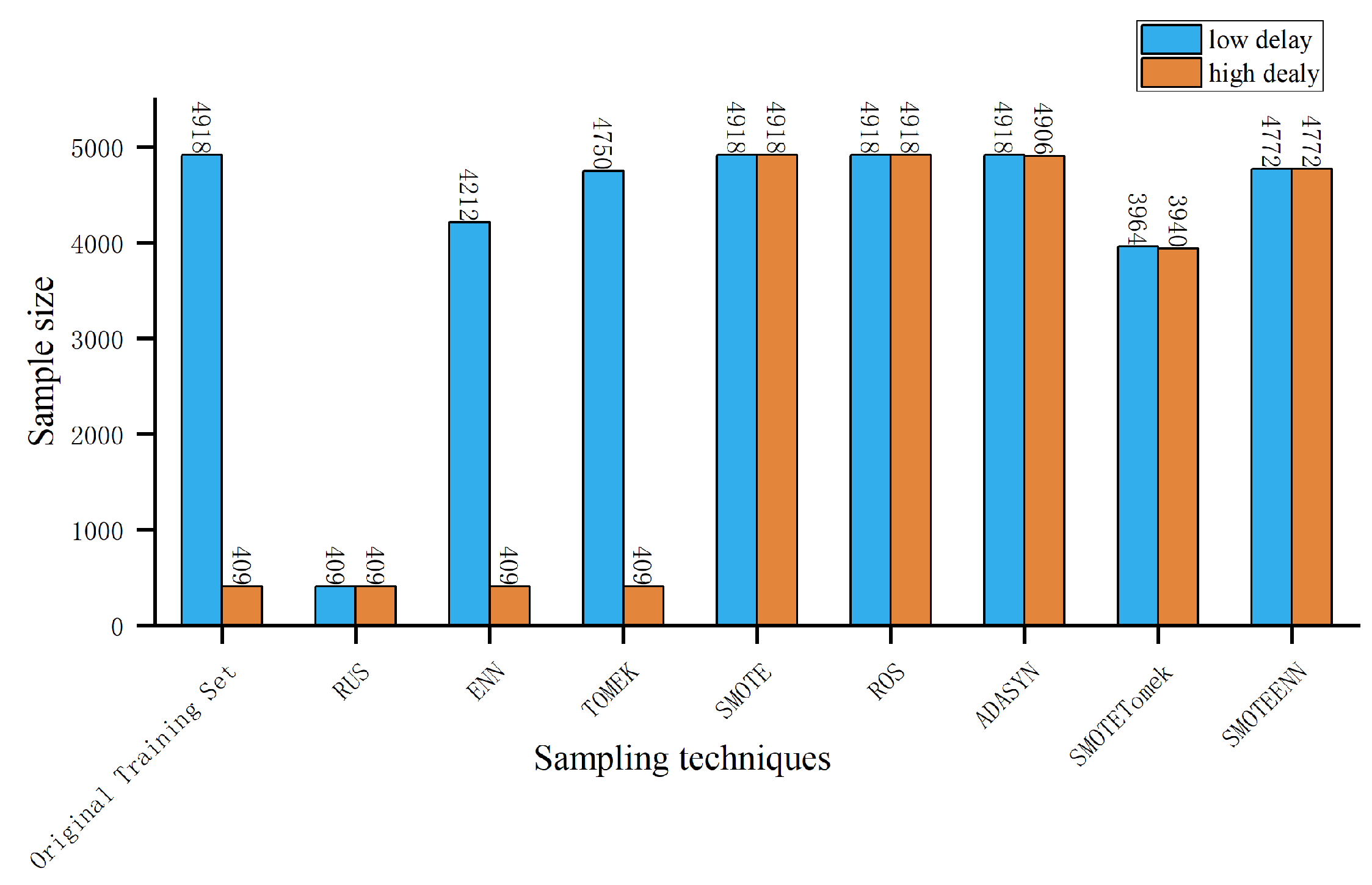

Table 1.
Prediction results of ADLCNN under multi-channel images with different resolutions.
| resolution | resolution | accuracy | label | Classification Report(%) | Confusion Matric | |||
|---|---|---|---|---|---|---|---|---|
| Precision | Recall | F1 | low delay | high delay | ||||
| RUS | GNB | 0.837 | low delay | 0.94 | 0.92 | 0.93 | 1942 | 167 |
| high delay | 0.24 | 0.30 | 0.26 | 123 | 52 | |||
| KNN | 0.673 | low delay | 0.96 | 0.68 | 0.79 | 1428 | 681 | |
| high delay | 0.14 | 0.63 | 0.23 | 65 | 110 | |||
| LLR | 0.720 | low delay | 0.97 | 0.72 | 0.83 | 1514 | 595 | |
| high delay | 0.18 | 0.75 | 0.29 | 44 | 131 | |||
| SVM | 0.680 | low delay | 0.97 | 0.67 | 0.80 | 1421 | 688 | |
| high delay | 0.16 | 0.75 | 0.26 | 44 | 131 | |||
| MLP | 0.699 | low delay | 0.97 | 0.70 | 0.81 | 1470 | 639 | |
| high delay | 0.16 | 0.72 | 0.27 | 49 | 126 | |||
| RF | 0.735 | low delay | 0.97 | 0.73 | 0.84 | 1548 | 561 | |
| high delay | 0.19 | 0.78 | 0.31 | 39 | 136 | |||
| AdaBoost | 0.733 | low delay | 0.98 | 0.73 | 0.83 | 1538 | 571 | |
| high delay | 0.19 | 0.78 | 0.31 | 39 | 136 | |||
| CNN | 0.780 | low delay | 0.98 | 0.78 | 0.87 | 1643 | 468 | |
| high delay | 0.23 | 0.81 | 0.36 | 33 | 142 | |||
| ROS | GNB | 0.871 | low delay | 0.94 | 0.92 | 0.93 | 1939 | 170 |
| high delay | 0.23 | 0.29 | 0.26 | 124 | 51 | |||
| KNN | 0.854 | low delay | 0.94 | 0.90 | 0.92 | 1891 | 218 | |
| high delay | 0.21 | 0.34 | 0.26 | 116 | 59 | |||
| LLR | 0.722 | low delay | 0.97 | 0.72 | 0.83 | 1522 | 587 | |
| high delay | 0.18 | 0.72 | 0.28 | 49 | 126 | |||
| SVM | 0.684 | low delay | 0.97 | 0.68 | 0.80 | 1429 | 680 | |
| high delay | 0.16 | 0.77 | 0.27 | 41 | 134 | |||
| MLP | 0.765 | low delay | 0.97 | 0.77 | 0.86 | 1618 | 491 | |
| high delay | 0.21 | 0.74 | 0.32 | 46 | 129 | |||
| RF | 0.898 | low delay | 0.94 | 0.95 | 0.94 | 2010 | 99 | |
| high delay | 0.29 | 0.23 | 0.25 | 135 | 40 | |||
| AdaBoost | 0.793 | low delay | 0.97 | 0.80 | 0.88 | 1685 | 424 | |
| high delay | 0.23 | 0.72 | 0.35 | 49 | 126 | |||
| CNN | 0.831 | low delay | 0.98 | 0.83 | 0.90 | 1762 | 349 | |
| high delay | 0.28 | 0.78 | 0.41 | 38 | 137 | |||
| SMOTEENN | GNB | 0.863 | low delay | 0.94 | 0.91 | 0.92 | 1914 | 195 |
| high delay | 0.23 | 0.33 | 0.27 | 117 | 58 | |||
| KNN | 0.786 | low delay | 0.95 | 0.81 | 0.87 | 1702 | 407 | |
| high delay | 0.19 | 0.53 | 0.28 | 82 | 93 | |||
| LLR | 0.717 | low delay | 0.97 | 0.72 | 0.82 | 1508 | 601 | |
| high delay | 0.18 | 0.74 | 0.29 | 45 | 130 | |||
| SVM | 0.696 | low delay | 0.97 | 0.69 | 0.81 | 1456 | 653 | |
| high delay | 0.17 | 0.76 | 0.28 | 42 | 133 | |||
| MLP | 0.806 | low delay | 0.97 | 0.82 | 0.89 | 1727 | 382 | |
| high delay | 0.23 | 0.66 | 0.34 | 60 | 115 | |||
| RF | 0.820 | low delay | 0.96 | 0.84 | 0.90 | 1769 | 340 | |
| high delay | 0.23 | 0.59 | 0.33 | 72 | 103 | |||
| AdaBoost | 0.791 | low delay | 0.97 | 0.80 | 0.88 | 1685 | 422 | |
| high delay | 0.22 | 0.69 | 0.33 | 55 | 120 | |||
| CNN | 0.773 | low delay | 0.98 | 0.77 | 0.86 | 1621 | 490 | |
| high delay | 0.23 | 0.84 | 0.36 | 28 | 147 | |||
Table 2.
Prediction results of ADLCNN under multi-channel images with different resolutions.
| resolution | accuracy | label | Classification Report(%) | Confusion Matric | |||
|---|---|---|---|---|---|---|---|
| Precision | Recall | F1 | low delay | high delay | |||
| 5x5 | 0.750 | low delay | 0.97 | 0.75 | 0.85 | 1586 | 525 |
| high delay | 0.20 | 0.74 | 0.31 | 46 | 129 | ||
| 25x25 | 0.766 | low delay | 0.97 | 0.77 | 0.86 | 1618 | 493 |
| high delay | 0.21 | 0.76 | 0.33 | 42 | 133 | ||
| 125x125 | 0.831 | low delay | 0.98 | 0.83 | 0.90 | 1762 | 349 |
| high delay | 0.28 | 0.78 | 0.41 | 38 | 137 | ||
Disclaimer/Publisher’s Note: The statements, opinions and data contained in all publications are solely those of the individual author(s) and contributor(s) and not of MDPI and/or the editor(s). MDPI and/or the editor(s) disclaim responsibility for any injury to people or property resulting from any ideas, methods, instructions or products referred to in the content. |
© 2023 by the authors. Licensee MDPI, Basel, Switzerland. This article is an open access article distributed under the terms and conditions of the Creative Commons Attribution (CC BY) license (http://creativecommons.org/licenses/by/4.0/).
Copyright: This open access article is published under a Creative Commons CC BY 4.0 license, which permit the free download, distribution, and reuse, provided that the author and preprint are cited in any reuse.


