1. Introduction
The mechanical properties of polymer composites are broadly scattered and require statistical treatments based on large data sets under static or cyclic loading conditions. The scatter is attributed to the accumulation of diffuse damage mechanisms that synergistically develop at different lengths and time scales and are eventually triggered by existing defects, including voids, fiber misalignments, and residual stress from the production process. Matrix cracking, fiber-matrix detachment, fibers and ply rupture, fibers buckling, and delamination progressively degrade the composites’ mechanical properties.
For these reasons, designing a composite structure requires more extensive mechanical tests than metal structures quantified in Ref. [
1]. Thus, the mechanical characterization of composites still represents one of the more expensive activities in structural applications, a requirement for which some industrial compartments do not have the resources or the time. Depending on the unicity of each composite structure, the different origins and locations of the damage mechanisms, rather than the propagation of a single crack, prevent any possibility of establishing sound inspection and maintenance criteria, as in metals. To this end, reliable simulation techniques may significantly reduce testing procedures. Two substantial approaches have been followed over the years. Mechanistic/hierarchical models are based on specific failure criteria depending on the length scales and the sequence/interaction of the damage mechanisms [
2,
3,
4,
5,
6]. However, the intricacy of damage accumulation mechanisms forces researchers to develop phenomenological models [
7,
8,
9,
10,
11,
12,
13,
14] without providing any information about the damage mechanisms, the events being predicted based on empirical criteria involving macro-stress components. The mechanistic and phenomenological approaches are not in contrast, the latter being addressed to supply analytical tools to perform reliability and scatter analysis on large databases of specific categories of composites subjected to particular loading conditions of fully developed structures. The Reifsnider’s "Critical Element Model" [
2], based on micromechanical representations of strength at increasing length scales, and the "Generalized Material Property Degradation Model" implemented by Shokrieh and Lessard [
4] belong to the same model’s category, representing an intermediate level of modeling the fatigue process between phenomenological and mechanistic approaches. In both cases, the phenomenological models from the macro level are combined with failure criteria and property degradation rules. However, neither Reifsnider’s nor Shokrieh and Lessard’s models account for the highly stochastic behavior observed in the fatigue life of composites, a prerogative of some phenomenological modeling approaches. The argument was discussed comprehensively by Vassilopoulos and Keller [
7] and y Philippidis and Passipoularidis [
8], where several models tested on the same set of fatigue life and residual strength data revealed that the statistical predictions at various stress levels and life fractions were largely unreliable. As a guide, this paper considers the fatigue’s stochastic nature in composites using a two-parameter formulation, inherently obeying the Strength-Life Equal-Rank Assumption (SLERA), and explicitly accounting for the stress ratio, R, [
9,
10,
11].
The SLERA states that if a sample of components could be tested for static strength and fatigue life expectancy, each member would occupy the same rank in the strength and life data sets. However, despite its potential powerfulness, the SLERA cannot be proved from one side, and its application to notched specimens is debated.
Based on the literature data, the reliability of the modeling procedure in predicting the fatigue life and the residual strength kinetics of open-hole (OH) laminates will be verified. Then, its robustness is further explored for variable amplitude loadings.
3. Model description
Our approach is based on a formulation that fulfills the following commonly accepted assumption:
- i)
A two-parameter Weibull distribution function represents the composites’ static strength.
- ii)
The fatigue limits seem unlikely in composite materials or irrelevant in the cycles encountered in practical applications. Thus, every load cycle potentially damages a composite structure and should be considered in life prediction calculations.
- iii)
The residual strength, that is, the strength measured on a sample subjected to cyclic loading under a given loading condition, slowly degrades in the first cycle’s decades and suddenly drops towards the maximum applied stress within a narrow cycle interval.
Moreover, the model obeys the Strength-Life Equal-Rank assumption (SLERA) formulated by Hahn and Kim [
16] and then by Chou and Croman [
17] :
"A specimen of a certain rank in the fatigue life distribution is assumed to be equivalent in strength to the specimens of the same rank in the static strength distribution".
In addition, the fatigue formulation described below simultaneously analyzes fatigue and static strength data, provided the loading rates used to measure the static strength are comparable with those in fatigue. This aspect will be discussed in what follows.
Our fatigue life formulation first developed was:
where N is the number of cycles to failure,
the maximum applied cyclic stress,
,
the static strength, and α and β the model’s parameters obtained by best fitting the fatigue data through Equation (1a) rearranged as follows:
We recall that the monotonic material strength, σ
0, is well represented by a two-parameter Weibull distribution. Therefore, the probability of finding a σ
0 value≤x is given by:
where γ is the scale parameter or the characteristic strength, and δ is the shape parameter.
Indeed, from Equation (1a) and (2), the original strength of the virgin samples, σ0N, fatigued until failure at cycle N*, can be recovered, and it should coincide with the statistical distribution of static strength, σ0.
Furthermore, coupling Equations (1a) and (2) one obtains:
From equation (3), given σ
max and R, the scatter in fatigue life exhibited by different samples conforms to the variability in monotonic strength. Thus, in principle, Equation (3) obeys the Strength-Life Equal Rank Assumption (SLERA) [16, 17] and accounts for the stochastic nature of strength and fatigue life. Solving Equation (3) for
N*, one obtains
from which the classical S-N curve for a fixed probability of failure
can be calculated, given the stress ratio, R.
Concerning the residual strength, once the parameters α, β, γ and δ are known, according to the developments already shown in [
18], the following distribution function can represent the strength evolution with cycles:
In Equation (4) is the strength of a sample fatigued n≤N cycles under given ad R; is the virgin strength of the sample with a given rank in the nominal static strength distribution function. Thus, Equation (5) describes the residual strength of a generic sample, as it degrades progressively from its virgin value, , to the maximum cyclic stress, , where failure occurs. Equation (5) can also be used to describe the statistics of the residual strength experimentally obtained at a given number of cycles, n, given and R.
Incidentally, rearranging Equation (5), when
, namely in the vicinity of failure, when
n ≅ N, Equation (1) is recovered as follows:
Equation (6) confirms that the fatigue life predictions, namely Equations (1a,b), can be regarded as an extreme case of the residual strength model, n according to Chou and Croman [
6].
4. Results and Discussion
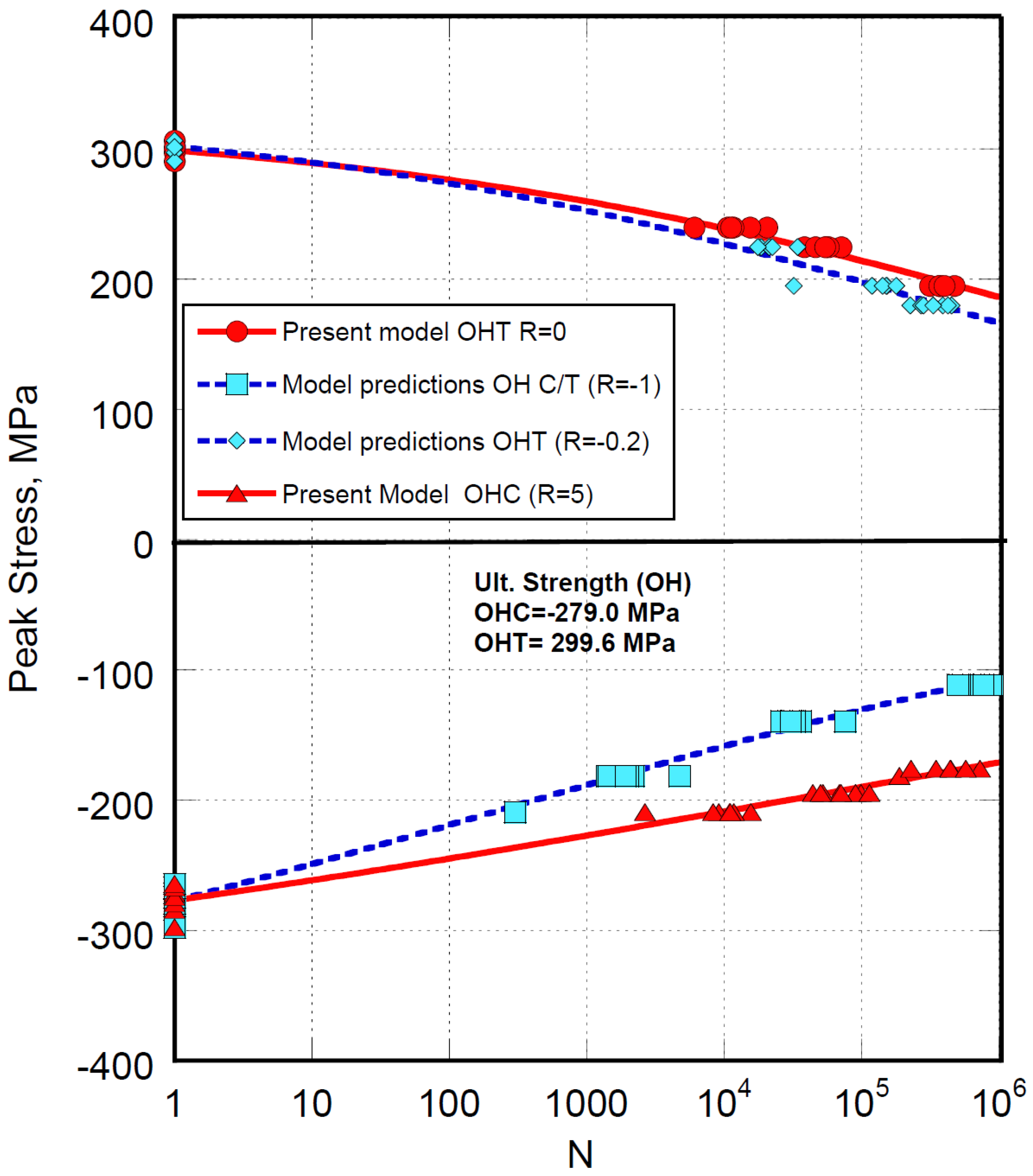
The fatigue life data of open-hole tension (OHT) and compression (OHC) samples at different stress ratios, R, are reported in
Figure 1. The data at R=0 and R=5 have been analyzed using Equation (1), allowing, by least square methods, the calculation of the two model’s parameters under pure tension and compression, namely α
t=0.074 and β
t=0.160 and . α
c=0.127 and β
c=0.174, respectively.
Figure 1.
Model predictions of fatigue life at different loading ratios, R, as indicated in the inset. The experimental data are taken from Ref.[
1].
Figure 1.
Model predictions of fatigue life at different loading ratios, R, as indicated in the inset. The experimental data are taken from Ref.[
1].
The deterministic nature of Equation (1) was converted to its statistical counterpart by applying the Strength-Life Equal Rank assumption (SLERA), namely, a longer fatigue life belongs to specimens exhibiting a higher static strength. To substantiate this statement Equation (1) was solved for
in Ref. [
11]:
According to the proposed procedure, the fatigue data under prevailing tension, namely R=-0.2 are predicted with the model’s parameter αt and βt. Moreover, despite the arithmetic symmetry of the stress ratio, the compression damage mechanisms developing at R=-1 prevail, with higher loading severity in compression, given that the distance from the static strength in compression is lesser than the counterpart in tension. Consequently, the data at R=-1 will be predicted with the parameters already obtained under pure compression, namely αc and βc.
From
Figure 1, the model predictions at R=-0.2 and R=-1 show that the fatigue data fall reasonably on the predicted curves.
As shown above, Weibull’s and model parameters are easy to obtain and remain fixed in predicting fatigue beyond the experiments. Thus, no adjustments will be allowed in what follows. We only mention that the stress ratio, ROHC, is normalized in modeling compression-dominated fatigue data. For instance, at ROHC=5, in Equation (1)
Equation (7) states that the static material strength, labeled by the symbol
to identify the calculated virgin strength, can be evaluated from the fatigue data, and the calculated statistical distribution coincides with the Weibull distribution of the measured strength, namely
. Thus, from Equation (7), the nominal static strength distribution, σ
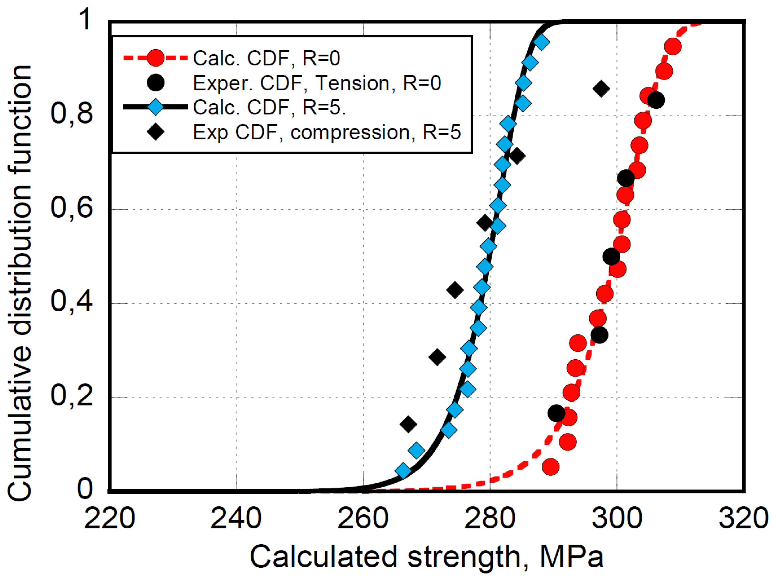
0N, of samples subjected to fatigue until failure can be recovered and reported in
Figure 2 for OHT at R=0 and OHC at R=5. The corresponding experimental static strength data set, also reported in
Figure 2, appears well described in both cases. According to a two-parameter Weibull statistical distribution, the nominal strength’s scale and shape factors are γ
t= 302 MPa and δ
t=53, and γ
c=281 MPa and δ
c=61, respectively.
Figure 2.
Experimental and calculates static strength distributions.
Figure 2.
Experimental and calculates static strength distributions.
It is worth mentioning that the application of Equation (7), namely the superposition of the experimental and calculated static strength, as shown in
Figure 2, is subjected to well-defined conditions. The literature frequently reports that static strength is measured at loading rates much lower than fatigue, or no information is given on the loading rates adopted to measure it. In those cases, the fatigue life model’s parameters, Equation (1), are obtained by excluding the static data. This argument has been largely debated so far [NIJISSEN]. The discussion is of primary importance in polymer-based composites where the matrix’ viscoelastic nature plays a dominant role at low content of fibers. The loading rate also influences the kinetics of damage accumulation since higher loading rates give rise to higher strength and longer life expectancy. Therefore, scaling procedures are needed when high frequencies are used to minimize the experimental characterization time to predict the responses of composite structures eventually subjected to lower in-service loading frequencies. This aspect is strictly connected with the random loading that composite structures may suffer during their service life. From above, it comes out that the complexity of fatigue response under CA loadings, including the SLERA assumption, can only be managed with coherent data sets and that models predicting the VA response are far to come. For instance, the loading rate, LR, in fatigue can be approximated by the following Equation:
where
f is the loading frequency. To roughly illustrate, with
,
R=0 and
f=10Hz, it results LR=5,000 MPa/s.Therefore, the static tests under load control for samples with a cross-section of 12 mm
2 require the application of 60,000 N/s. If the elastic modulus along the direction of the applied load is 25,000 MPa, then, under displacement control, the strain rate is
=0.2 s
-1, and the static strength of samples of length L=100 mm should be measured at a cross-head speed of 120 mm/s. However, when dealing with high-performance carbon fiber composites, the stacking sequence consists of layers oriented along the load direction. In those cases, the strength sensitivity to the loading rate is very low []. For instance, unidirectional carbon fiber composites’ strength shows negligible loading rate dependence. In all the other cases, measuring the strength as a function of the strain rate is mandatory.
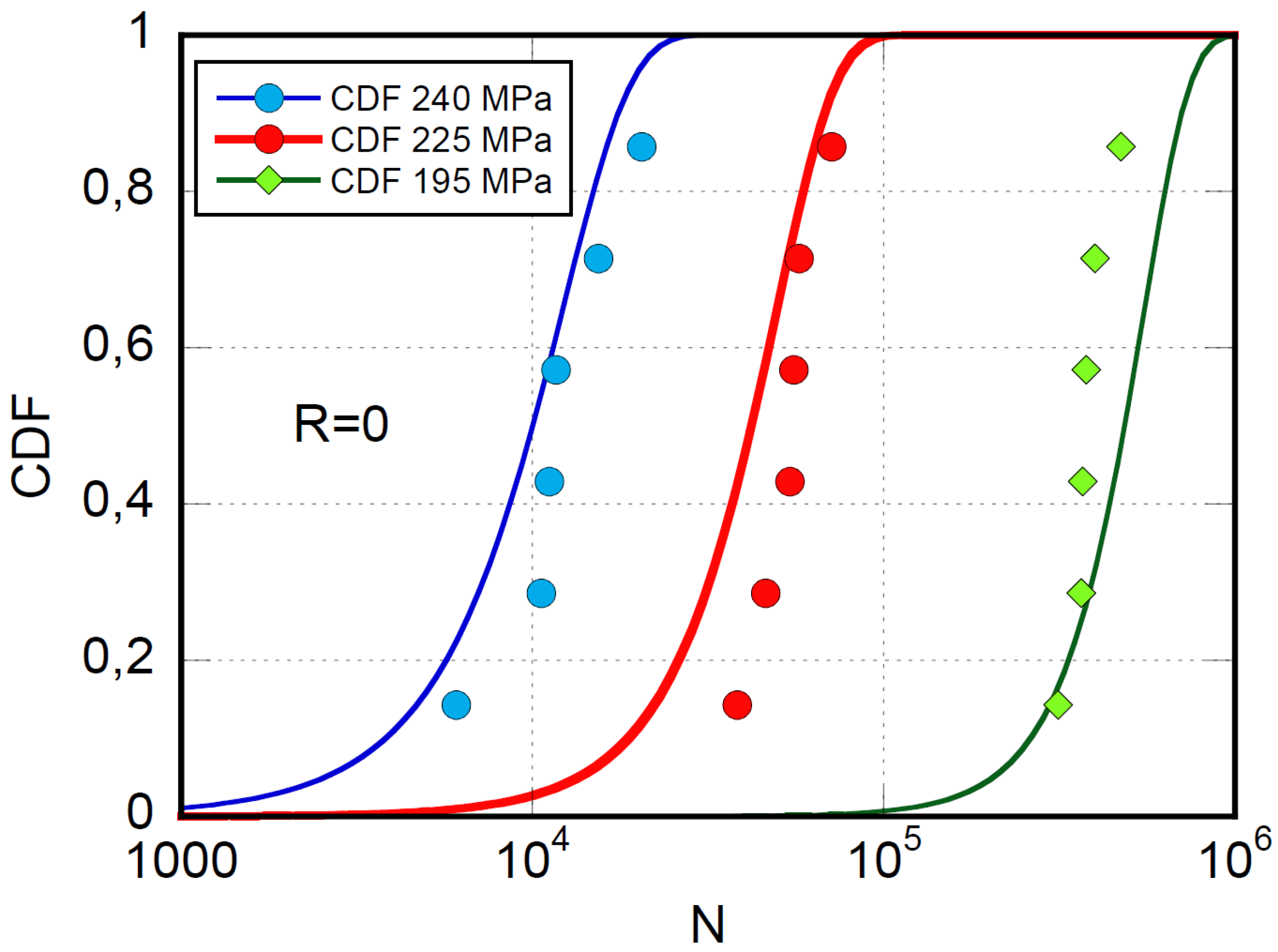
A further implication of the modeling procedure is described by Equation (3), describing the statistics of failure cycles, given
and R. With the model’s parameters already found, the experimental data at R=0 and
and the model’s predictions are reported in
Figure 3.
Figure 3.
The fatigue life distribution function at different maximum stresses and R=0.
Figure 3.
The fatigue life distribution function at different maximum stresses and R=0.
With the relatively narrow data set available, we consider satisfying the predictions. Not reported here, the model’s capability to replicate the experimental distribution of fatigue data was verified at different stress ratios, R, with the same quality. Thus, Equation (3) establishes a robust analytical correlation between the static strength and the fatigue distribution functions.
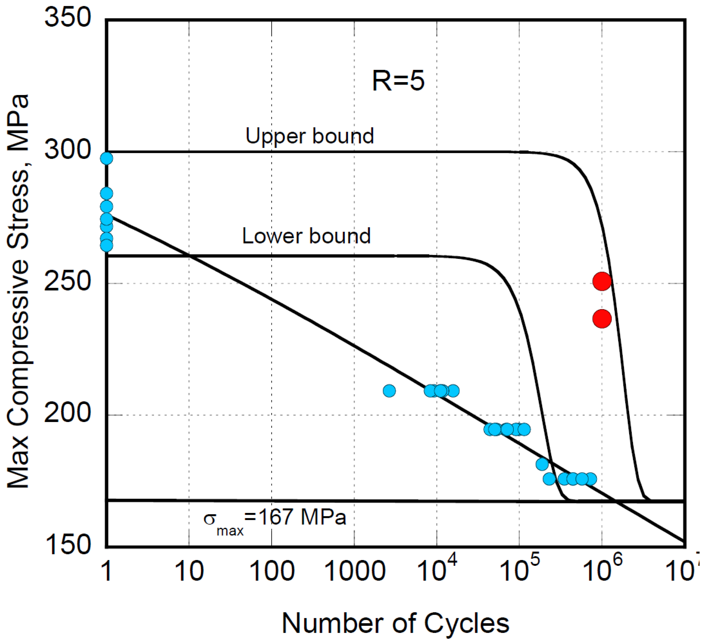
Moreover, based on Equation (5), the statistical distribution of residual strength can be predicted under different loading conditions. To illustrate, let us first recall that, given the loading conditions, namely,
and R, stronger samples will fail at a higher number of cycles, according to the strength-life-equal rank assumption (SLERA). Accordingly, the residual strength data should remain confined between the strongest and weakest samples’ strength degradation curves routinely taken from the extreme tails of the static strength’s cumulative distribution function, namely when F=0.95 and 0.05, respectively. To this end,
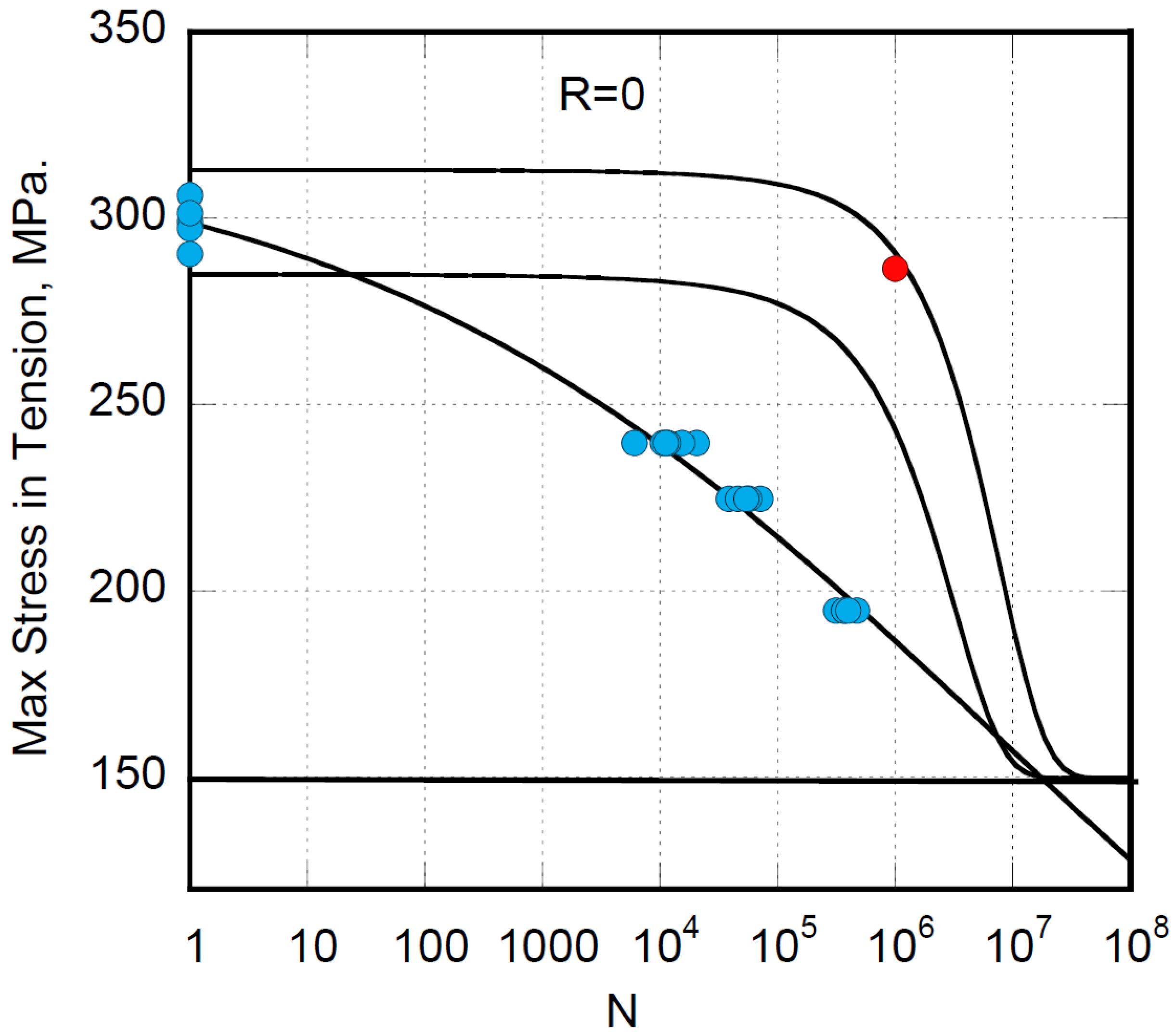
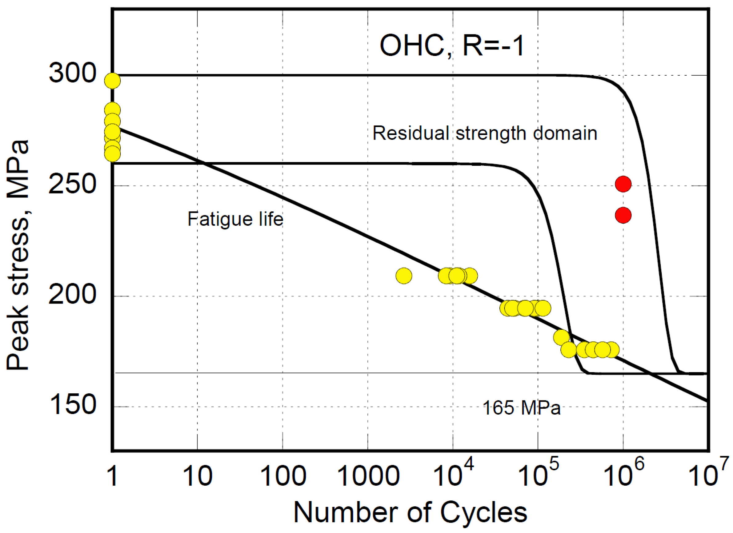
Figure 4,
Figure 5 and
Figure 6 report the model predictions for (OHT) at R=5, R=0, and R=-1 respectively. As expected, the residual strength data taken after a million cycles are well within the domain confined between the boundaries referred to as upper and lower bounds, describing the strength degradation kinetics of the weaker and stronger samples. Furthermore, at R=-1, the substantial degradation mechanisms are debited to macro stresses acting in compression and tension. However, it should be mentioned that even if the nominal cyclic loading severity in tension and compression is the same (
) the damage accumulation and strength degradation kinetics result in compression failure. In the framework of our approach modeling it is evident that, given σ
max and R, the strength degradation kinetics depend on the "distance" from the virgin strength, which is lower in compression than in tension for the laminate under study. Thus, the predictions at R=-1 use scale and shape factors, γ and δ, of the cumulative distribution function coming from the calculations based on Equation (1) applied to the pure compression data, namely , R=5. Such deliberate approximation is strong proof of the approach’s robustness, even if deeper insight can be obtained by recovering the shape and scale factors from the data at R=-1 using Equation (7). Herein, we are just proposing a general procedure that, at first glance, appears promising. Furthermore, it is worth mentioning that in Equation (5), describing the continuous upper and lower bound curves of
Figure 4,
Figure 5 and
Figure 6 delimiting the pertinent residual strength domain, the parameters α
c, β
c, γ
c, and δ
c are already fixed and come from a different data set while
n is the running variable. Thus, the procedure so far illustrated is entirely predictive.
In summary, the fatigue life, the statistical distribution of cycles to failure, and the residual strength can be managed simultaneously through a single set of parameters, namely, α, β, γ and δ, provided the sign of the prevailing macro stress is recognized. For instance, in composites, the dominant fracture occurs in compression when R=5 and R=-1, where both tension and compression stresses are in play.
Figure 4.
Residual strength (red circles) prediction at R=5.
Figure 4.
Residual strength (red circles) prediction at R=5.
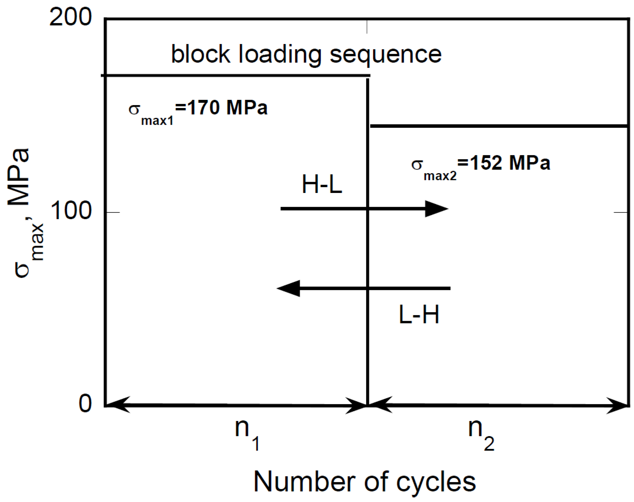
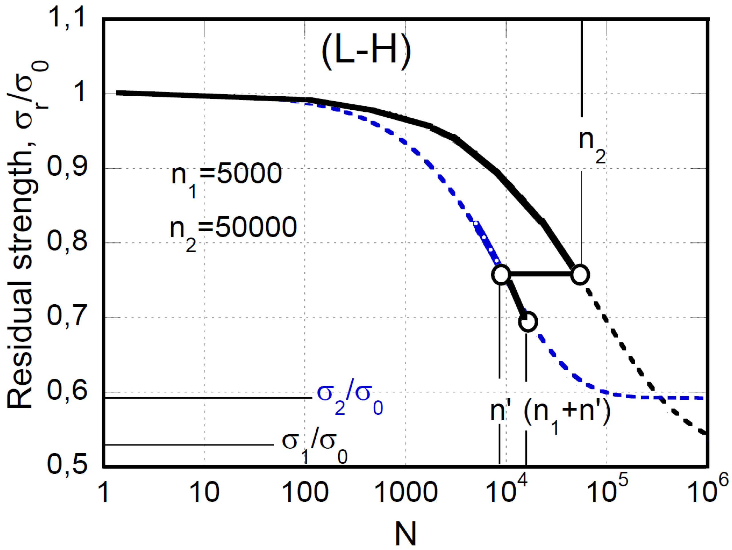
It should be underlined that only two of the four parameters come from the fitting procedure, namely α and β, while γ and δ come from the experimental statistical distribution of strength data. In the framework of our approach, the four parameters represent the material’s fingerprint, even limiting our discussion to the experimental data obtained under constant amplitude loading. A different story and complexity emerge when random loadings are in play. To this end, in what follows a preliminary approach to circumvent the complexity of fatigue response under variable amplitude loadings. The discussion is confined to the simplest case of two-block loading. The blocks have different durations, namely 50,000 and 5,000 cycles, and loading is performed at constant amplitude at a given stress ratio, R, and different maximum applied stress,
, respectively, as depicted in
Figure 7, where the schematic of high-to-low (H-L) and low-to-high (L-H) loading sequences is reported.
Figure 5.
Residual strength (red circles) prediction at R=0.
Figure 5.
Residual strength (red circles) prediction at R=0.
Figure 6.
Residual strength (red circles) prediction at R=-1.
Figure 6.
Residual strength (red circles) prediction at R=-1.
The sequence is arbitrary, yet it allows discussing Miner’s rule for damage accumulation in detail when variable amplitude loadings are in play. Symbolically, the Miner’s rule can be expressed as:
where
ni is the number of cycles elapsed under given CA loading condition, and
Ni is the number of cycles to failure under the same loading condition. For the case under study, the number of cycles to failure were
N()≈ 1x10
5 and
N() ≈ 110
6, respectively, and the damage calculated through the Miner’s rule is D≈0.1, regardless of the loading sequence, as expected. In
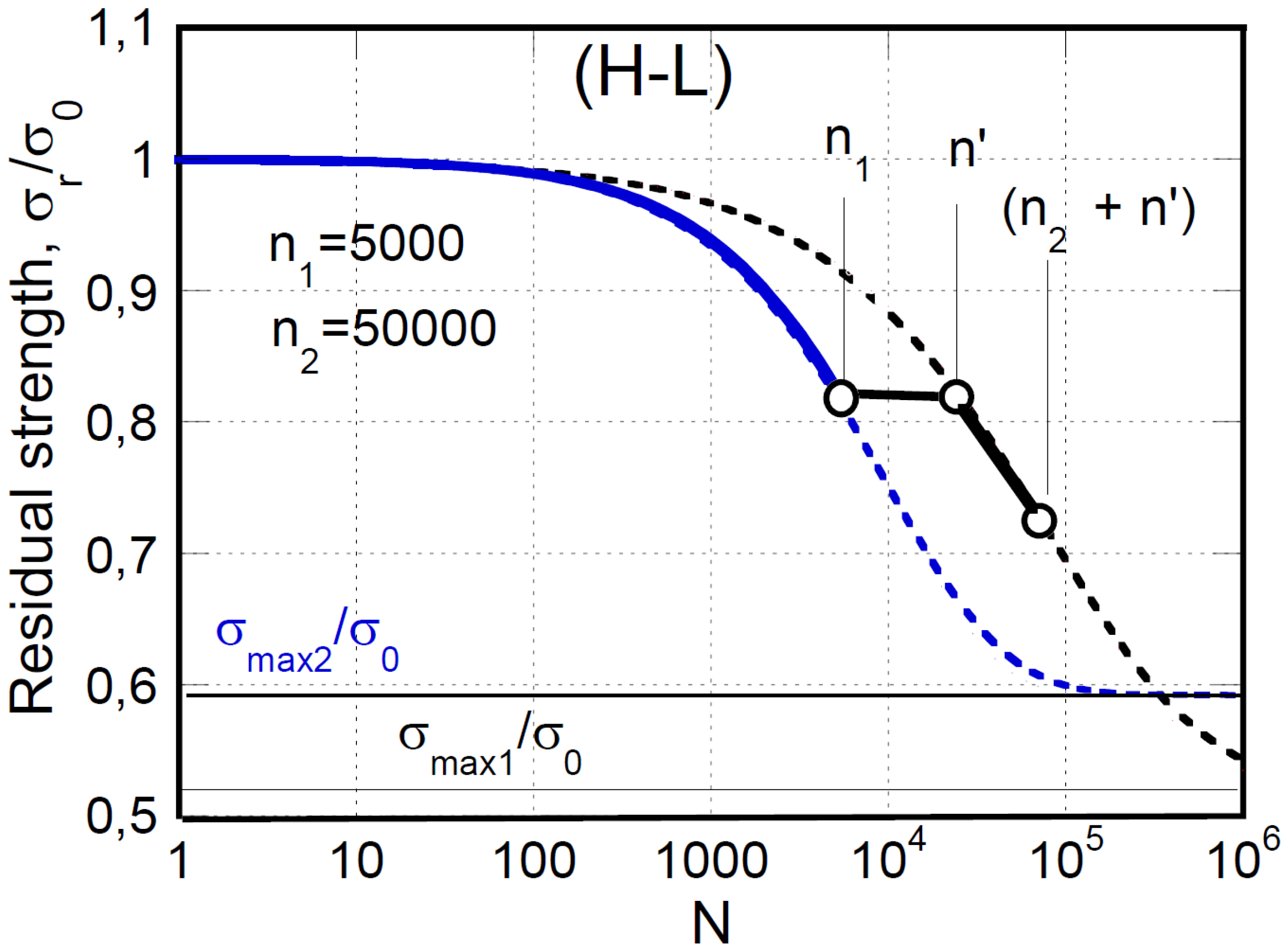
Figure 8, the strength degradation path for H-L sequence is schematically described. Starting from the normalized mean static strength, i.e., σ
r/σ
0=1, the strength degrades following the baseline degradation curve at higher applied maximum stress,
, until the end of the first loading block when n=5000. The second bloc starts with the strength reached at the end of the first block and from the adjourned number of cycles, n’. The strength degradation proceeds for n
2 cycles following the degradation curve at a lower stress,
. Similarly, the response to the ascending L-H sequence is illustrated in
Figure 9.
Figure 7.
Schematic of the H-L and L-H block cycle sequence.
Figure 7.
Schematic of the H-L and L-H block cycle sequence.
The effect of the loading sequence can be quantified employing the damage, D, accumulated within the materials [
18,
19] , defined here as follows:
Where
is the residual strength variation under the
ith loading block characterized by
and
Ri, and
is the total degradation extent under the same loading condition. The damage so far defined is compared with the one calculated through Miner’s rule, and the data are reported in
Table 2.
Figure 8.
Schematic of two-block H-L strength degradation path.
Figure 8.
Schematic of two-block H-L strength degradation path.
Figure 9.
Schematic of two-block L-H strength degradation path.
Figure 9.
Schematic of two-block L-H strength degradation path.
Table 2.
The damage accumulation predictions based on Miner’s rule and Equation (10).
Table 2.
The damage accumulation predictions based on Miner’s rule and Equation (10).
| |
Miner’s rule |
Equation (10) |
| H-L sequence |
0.1 |
0.63 |
| L-H sequence |
0.1 |
0.65 |
Our results evidence the fault of the Miner’s rule. First, it cannot discriminate the loading sequence; secondly, the accumulated damage appears highly unconservative. Nonetheless, the Miner’s rule is still used in a series of commercial software and as a reference in predicting the damage accumulation with different formulations [
20]. Our approach discriminates the loading sequence, and the predicted damage is at least more conservative regarding Miner’s rule.
Finally, the utterly arbitrary loading sequence adopted herein allows the use of our approach cycle-by-cycle for random loadings.
