
Submitted:
16 October 2023
Posted:
17 October 2023
You are already at the latest version
Abstract
We report on the study of the temperature dependence of the response of a BSO crystal based polarimetric current sensor with spectral interrogation. Two possible interrogation schemes are discussed. The spectral dependence of the optical rotation along the crystal caused by temperature and current changes has been investigated and approximate dependences for the sensitivities to current SI and temperature ST have been derived. A mixed term in the response with spectral interrogation has been revealed, the elimination of which is done by tracking wavelength shifts of two distinct extrema in the polarimetric response. A temperature independent second degree equation for the current changes as a function of the spectral shifts has been derived and tested.
Keywords:
magnetic field sensor
; current sensor
; temperature independent measuremenents
; polarimetry
; fibre optic sensors
; spectral interrogation
1. Introduction
Faraday effect based electric current and/or magnetic field fiber optic sensors have been known, developed and commercialized [1] for quite some time for the purposes of the power industry [2] and special applications [3]. These sensors are based either on the Faraday effect in the fiber itself, or in bulk materials [4] which use optical fiber transducers such as fiber Bragg gratings (FBG), interferometers or refractometers [5,6,7,8,9,10,11] in combination with the magnetic field sensitive materials. These sensors are characterized by specific advantages / disadvantages and varying simplicity and complexity.
Among the simplest and most straightforward solutions are the polarimetric sensors using magneto-optical materials such as BSO (Bi12SiO20) and BGO (Bi4Ge3O12) crystals because of their high Verdet constant and whose wavelength dependence has been accurately measured and well known [12,13]. The first polarimetric fiber optic sensor using BSO/BGO crystals [14,15], however operate at a single wavelength and detect amplitude changes of the polarimetric response. These crystals are also temperature dependent [16,17] which presents a limitation on the performance of the sensor. To account for temperature dependence, detection at two wavelengths has been proposed [18] or the temperature dependence of the BGO crystal has been taken into account [19]. The problem with the temperature dependence for the other types of the current sensors has been addressed in different ways depending on the interrogation scheme and the magneto-sensitive material by either temperature compensation [18,19,20,21,22,23] or simultaneous magnetic field and temperature measurement in the case of magnetic field sensors with spectral interrogation [24,25,26,27,28].
We have recently shown [30,31] that the well-known fluorescence in BSO crystals [32] can be used to generate under ultraviolet or white LED excitation a broad spectrum which serves as broadband source for a polarimetric scheme with spectral interrogation. We have also reported [33] that the BSO crystal based polarimetric sensor exhibits a wavelength dependent temperature dependence.
In the present work we measure the optical activity of a BSO crystal at different temperatures, currents and wavelength and establish the spectral and temperature dependence of the intrinsic and magnetic field induced polarization rotation. We show that the spectrally interrogated polarimetric fiber optic current sensor using a white LED can be used eliminate the temperature dependence in the measurement of the electric current.
Section 2 presents the general experimental set-up, the principal of operation and the two possible interrogation techniques. Section 3 is devoted to the measurement of the spectral dependence of temperature-influenced optical activity from which we derive the spectral, temperature and current dependences of the sensitivities to current and temperature. To eliminate the temperature dependence we use the spectral shifts of two extrema of the polarimetric spectral response and derive an expression for the current changes. The performance of the current sensor is simulated numerically.
2. Principle of operation and experimental arrangement
2.1. Experimental set-up
The experimental set-up in Figure 1 was used to generate a broad spectrum from 520 nm to 800 nm in the BSO crystal and to observe the spectral distribution of the polarimetric responses which is given by the expression [31]:
In (1) θ and α are the polarizer and analyzer orientations and
is the accumulated phase along the circularly birefringent BSO crystal whose length is L and Δβ = βL-βR is the propagation constant difference between the left and the right circularly polarized waves along the crystal. This difference is both wavelength and temperature dependent and is expressed as [31]:
In (3) ρ (deg/mm) is the optical rotatory power of the crystal and the additional rotatory power ρF = VBB caused by the Faraday effect, B being the magnetic field and VB the Verdet constant. The wavelength dependences of ρ(λ) and VB(λ) is well known [12,13], both decrease with wavelength and VB is proportional to ρ [17]. Temperature dependences, however, have been insufficiently studied and further in the paper we present more detailed results. Inserting (3) and (2) into (1) we have for the wavelength and temperature dependent intensity I(λ,T) [30,31].
Φ(B,T,λ) being the total phase in the polarimetric response. The typical spectral responses of a polarimetric sensor to changes of the polarizer/analyzer orientations and to current (magnetic field) are shown in Figure 2.
The plots show that the particular position of the modulated pattern can be fine-tuned by changing the orientation of the analyzer / polarizer via the θ−α term. The changes of the measurand (current / magnetic) field and for that matter of temperature lead to shifts of the polarimetric response as shown in Figure 2b)
2.2. Principle of operation and sensitivities
Unlike the single wavelength polarimetric arrangement [14] in which the intensity (4) is measured, in our arrangement we observe by a spectrometer the whole spectrum which exhibits an oscillatory response. Since both ρ(λ) and VB(λ) decrease with wavelength the period of the wavelength dependent response Λ (which is the free spectral range – FSR) increases with wavelength. As the angle between polarizer and analyzer can be varied, we can tune the phase 2(θ−α) and thus fix the position of the polarimetric response.
2.3. Interrogation detection techniques
There are two detection techniques that can be used to detect the changes in the polarimetric spectral response. In the first we track the wavelength position of a minimum λm or a maximum λM, as the magnetic field/elecric current changes. Thus, the wavelegth shifts δλM = δλM - δλM,0 of a maximum and δλm = δλm - δλm,0 of a with respect to some wavelength positions at I = 0 A and T = T0 are tracked. In the second, we observe the intensities that are +π/2 and –π/2 phase-shifted with respect to an extremum IM+ and I M- for a maximum or Im+ and I m- for a minimum and calculate the differences and the sums of intensities that are π-shifts with respect to one another: ΔM = IM+ - I M-, ΣM = IM+ + I M- and Δm = Im+ - I m-, Σm = Im+ + I m- and then calculate the normalized differences NM = ΔM / ΣM and Nm = Δm / Σm which change with current/magnetic field and temperature.
2.3.1. Extrema wavelength shifts
In this case for a given magnetic field B (or current I) and temperature T, the wavelengths λM,k and λm,k of the k-th maximum and minimum of the polarimetric response are those for which the phase Φ from (4) is:
min
and the phase change ΔΦ is then
When we track the shifts Δλk of an extremum (at λM,k or λm,k) with respect to the position for I = 0 (B = 0) caused by changes of the magnetic field (or current) ΔB (or ΔI) and of the temperature ΔT, resultant phase change ΔΦ of the ΦM or Φm is zero because the condition (5a) for the tracked extremum remain the constant i.e. ΦM = 2kπ = const and ΦM = 2kπ = const. The expression (5b) becomes null and solving with respect to Δλ we obtain:
where SB and ST are the sensitivities to magnetic field and temperature changes
In (5) and (6) λk is either λM,k or λm,k as instantly tracked and Δλ k is the wavelength shift of the extremum from the initial value λk,0 for which I = 0 and T = T0 This type of interrogation is illustrated in Figure 3a). Both the magnitude and the sign of the current / magnetic field can thus be measured. Figure 4a) shows the wavelength shifts of the extrema from the response in Figure 3a) which prove to be linear with wavelength, while Figure 4b) shows the correspondingly measure sensitivies which increase with wavelength [30,31].
2.3.2. π-shifted normalized differential response
In this case the intensities and of the polarimetric response around the k-th extremum (and ) that are π-shifted to each other can be defined as:
The normalized differential responses around the k-th maximum or the minimum are defined as:
In the initial state =, but when the polarimetric response shifts to the right the difference becomes positive and vice versa as shown illustrated in Figure 3b) by the red and blue vertical arrows. Therefore, both the amplitude and the sign of the current/magnetic field can be detected. The sensitivities to magnetic field/current and to temperature are defined in this case as:
Figure 5 presents the responses of the normalized differential signals according to the π-shifted interrogation technique. As is seen the responses are with different sensitivites though not quite linear as those from Figure 4. The sensitivity in this case shows similar wavelength dependence as with the first interrogation method (Figure 4b).
3. Experiment and results
3.1. Experimental set-up
To study the possibility for temperatur corrected current measurements we need to know the dependences of the optical activity and the Verdet constant on the wavelength ρ(λ), V(λ) and on temperature ρ(Т), V(Т). The experimental set up used to perform the needed measurements is shown in Figure 6.
The light source is a white halogen lamp (Ocean Optics) and the spectrometer was an Avantes VASPEC-ULS2048CL-EVO, (0.5 nm resolution and a 400 nm to 900 nm range). The light from the source is coupled to 600 μm large core quartz-polymer lead-in fiber, collimated at its output, polarized by a polarizer through an angle θ, traverses the BSO crystal, passed through an analyzer oriented to an angle α, and focused to and same type of a lead-out fiber. Alternatively, for current and temperature measurements the white light halogen lamp was replaced by a white LED. The BSO crystal (4 x 4 x 25) is placed in an aluminum holder and is heated/cooled using a thermoelectroc cooler (TEC). Polarizer was fixed with transmission axis along the horizontal axis of the crystal. Only the analyzer was rotated during measurements of the optical activity and its temperature dependence. The temperature could be varied from -32°C to 62°C. The power supply could provide a current in the range from -30A to +30A (±0.1 A) which fed the solenoid coil to create a homogeneous magnetic filed along the BSO crystal as shown in Figure 6.
3.2. Results on optical activity measurements
Using the set-up shown in Figure 4 we performed a sequence of measurements in which we change the temperature T, current I across the solenoid and measure the output angle of rotation of the polarization at a particular wavelength λ. The measurements were done by compensation of the polarization rotation via turning the analyzer angle j so that a given minimum at a specified wavelength in the polarimetric response (Figure 2) remains at the same position which means that for a given minimum (k = constant) as
The sequence of measurements is as follows:
- i)
- wavelength among the following 540 nm, 570 nm, 600 nm, 630 nm, 660 nm and 690 nm is chosen starting from the highest value. In the absence of magnetic field (I = 0A) and at room temperature (≈22°C) the analyzer is rotated until a minimum of the response coincides with the chosen wavelength of measurement (690 nm for example).
- ii)
- For a chosen value of the wavelength λk, a value of the current is fixed between I = -30A and I = 30 A. For a fixed value of the current the temperature is varied between T = -30°C to 60°C and for each temperature the analyzer is rotated to compensate for the temperature and current induced phase changes (26) due to the ρ(λk,T), VI(λk,T) and I and the particular value for φ is found.
- iii)
- After the temperature is scanned, a new value for the current for the same wavelength is set and then the temperature scanning is repeated.
- iv)
- After all currents are scanned, the next wavelength is chosen and the procedure from i) to iii) is repeated.
The results obtained provide the possibility for the following analysis to be performed. First, the only spectral and temperature dependence is in the optical activity and the Verdet constant and second, neither of them depends on the current, so the compensation angle is represented as.
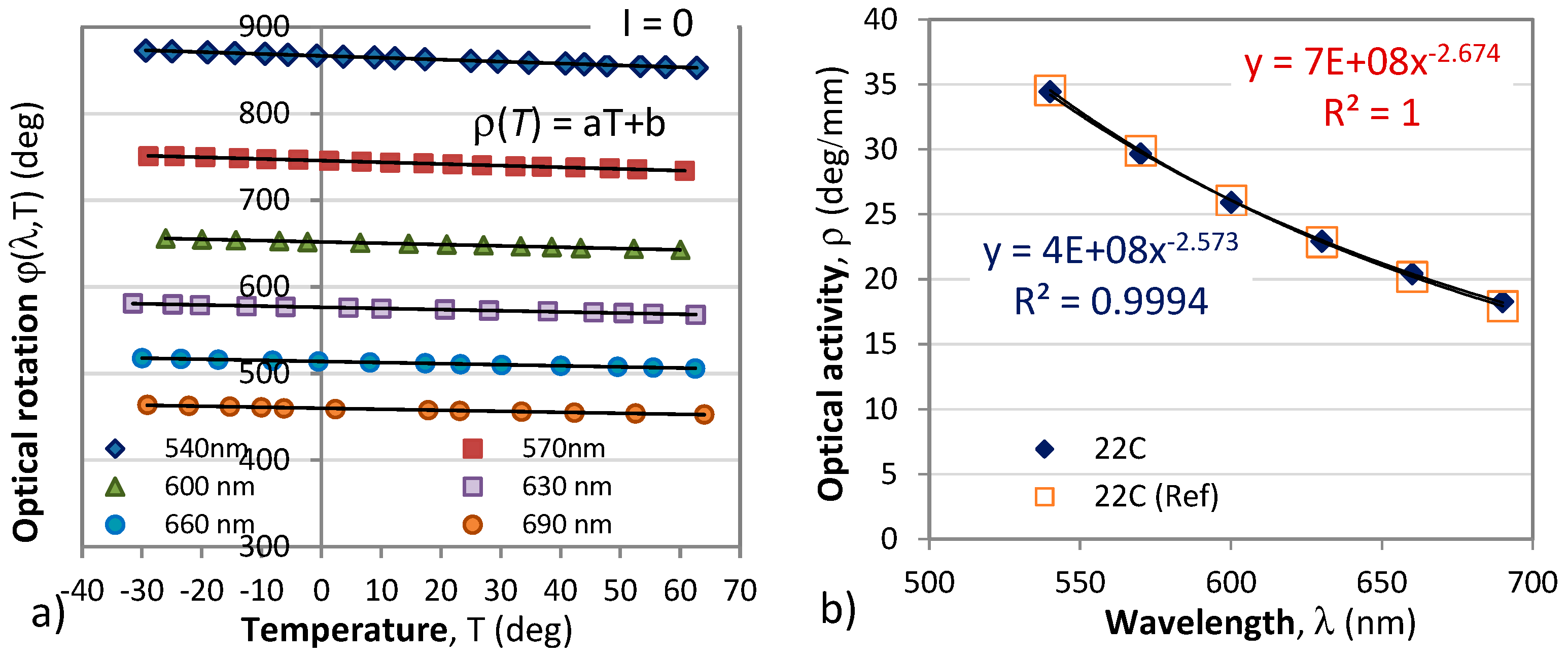
Second, we analyze the results for I = 0, which reveal the dependences ρ(λk,T), so we have
Figure 5a) shows a plot of the rotation angle caused by optical activity vs. temperature for the above six wavelengths in the absence of a magnetic field (I = 0). As is seen from this figure, the optical rotation linearly reduces with temperature and can be represented in the form:
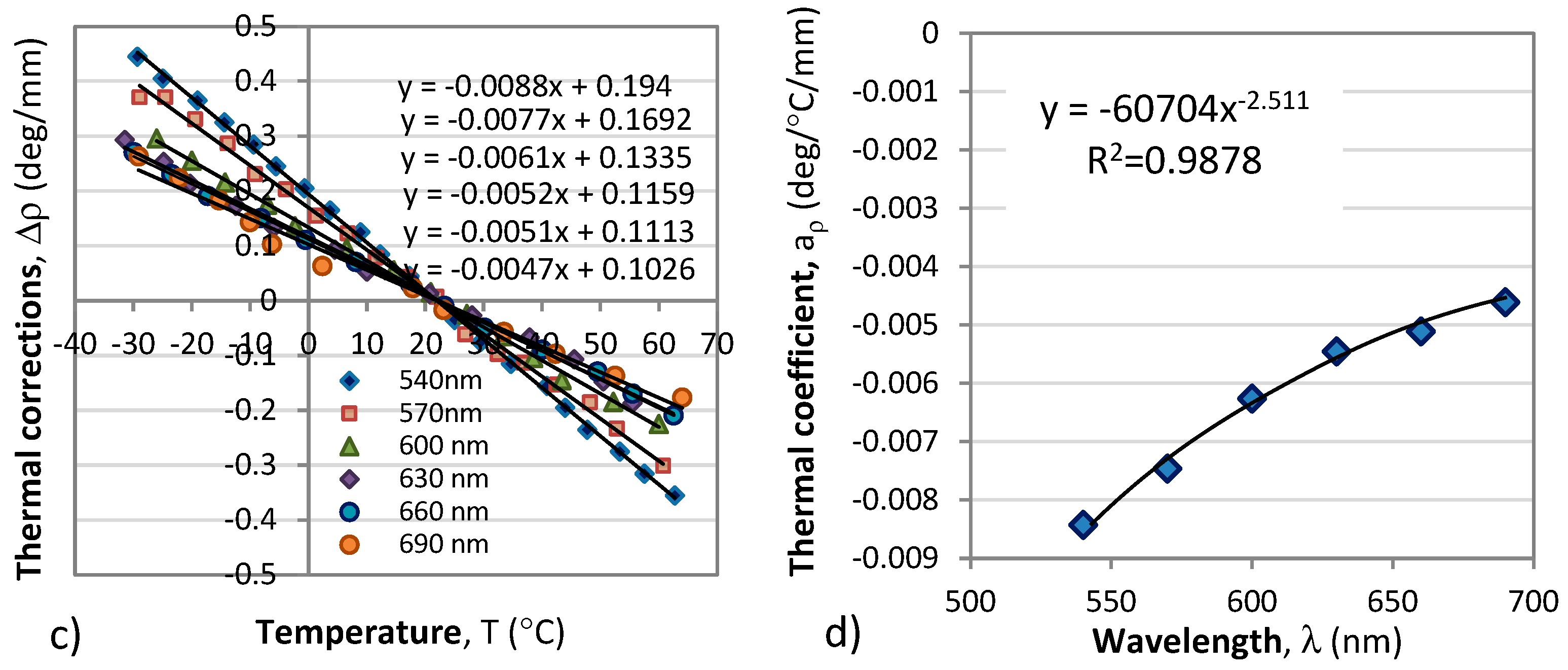
where the thermal coefficient aρ(λ) that determines the slope of the lines in Figure 5a) as well as the optical activity ρ0 are wavelength dependent.
Figure 7.
Spectral and temperature dependence of the optical rotation without magnetic field (I = 0): a) rotation angle vs. temperature at different wavelengths; b) wavelength dependence of the optical activity ρ(λ) at room temperature (22°C); c) temperature corrections Δρ to the optical activity with respect to the response from (b) at room temperature; d) thermal coefficient aρ.
Third, from the measurements at different temperatures in the -30°C to 60°C range for different currents from -25A to +25A we can retrieve the optical rotation VI.L (deg/A) due to the magneto-optic effect and its wavelength dependence presented in Figure Figure 8. In that figure we plot VI(λ).L for three temperatures -30°C, 0°C and 60°C and it is seen that the temperature deviations vary randomly in either directions. The relative error due to temperature-dependent deviations of the magneto-optic activity varied with wavelength and on the average was found to be ≈ 0.7%. The relative error due to temperature-dependent deviations of the magneto-optic activity varied with wavelength and on the average was found to be ≈ 0.7 %. We thus conclude that
where ε(T) is a negligible thermally dependent correction
3.3. Approximations
The experimental plots obtained for ρ0(λ), aρ(λ) and V(λ) are found to be sufficiently well approximated by power law functions namely as:
Based on the above we can write (14) as
and for λ from 540 nm to 700 nm and T from -30°C to +60°C the power law approximations (31) can be used for all wavelength dependences:
4. Simultaneous current and temperature measurement technique
4.1. Sensitivities to current and temperature
To realize temperature corrected current measurement the non-linear power-law approximations for aρ(λ), ρ0(λ) and V(λ) are simplified according to the following procedure:
- i)
- Use the power law approximations (31) to study the responses to current and temperature changes and determine the sensitivities SI and ST.
- ii)
- Study the wavelength, temperature and current (magnetic field) dependences of SI and ST.
- iii)
- Develop a method for simultaneous two parameter measurement.
We first model the white light LED spectral distribution used in the sensor by a shifted Gamma function defined as [31]:
Taking into account (31) and (32), the intensity distribution at the analyzer can be represented as
The parameters for the Gamma function are as follows: λ0 = 515 nm, α = 3.75 and β = 27. The theoretical fit using (17) a real polarimetric responses at analyzer angle 0° is presented in Figure 7 and is compared to the response at 60°.
The full differential of the phase per unit length dΦ/2L is found from (3b)
In case of spectral interrogation by extremum tracking dΦ =0 and we find for δλ as
As the power law expressions are nonlinear we proceed to the second step outlined above and perform a study of the wavelength, temperature and current (magnetic field) dependences of SI(λ,I,T) and ST(λ,I,T). To do that we change the current I at a constant temperature T, and then change temperature for constant current and measure the resulting wavelength shifts of the minima and maxima in the distribution from Figure 9. The we plot the dependence of Δλ vs I for different temperatures for each extremum, as well as Δλ vs T for different currents, from which we determine the needed sensitivities.
Figure 10 shows the wavelength changes of four minima
The wavelength dependence for the current sensitivity SI(λ) is experimentally confirmed in ref [31] and as we see at each wavelength the Δλ(I) dependence is linear. So is the SI(λ) over the range of wavelengths above 550 nm, though weakly dependent on temperature.
As is seen from Figure 10b) the sensitivity to current is linearly dependent on the wavelength and can be represented as follows
The linear fits of each of the coefficients presented in Figure 10c,d) below can be represented as follows:
The wavelength shifts of the four minima with temperature and the temperature sensitivity on the wavelength ST(λ) at different current levels is presented in Figure 11.
From Figure 9 b) it is seen that the temperature sensitivity ST(λ,I) is linearly dependent on the wavelength and can be written as:
where the B0(I) and B1(I) are also linear functions of the current Figure 9c) and 9d) and are written as:
As follows from (21)
4.2. Two points method for simultaneous two-parameter measurement
In this form the unknown quantities are the current I and temperature T and after insertion of (22b) into (22a) and of (23b) into (23a) we obtain after some rework for the k-th extremum tracked we can write
Where
Equation (24) contains a mixed term proportional to ΔIΔT. To eliminate the temperature dependence we chose two extrema wavelengths choose λ1 and λ2 (k = 1, 2) to track to our choice. By varying the orientation of the analyzer we can fine tune the position of the pattern. Eq. (24) then is written for each of the wavelengths as:
Solving (26a,b) with respect to the mixed ΔT term and eliminating the temperature dependence leads to a quadratic equation with respect to the current:
Where
Solving (37) with respect to ΔI yields
The electric current measurement procedure runs thus as follows:
- i)
- The coefficients from Table 1 are substituted in (25).
- ii)
- By fixing the position of the analyzer with respect to the polarizer, a desirable position of the spectral response is fixed for I0=0 and T = T0 which quantities are also to be inserted in (35). The two extrema whose shifts are to be monitored are fixed and under these conditions their values λ10 and λ20 are measured and substituted in (25) as well.
- iii)
- The instant values of the extrema λ1 and λ2 are measured over regular intervals Δt are inserted into (25) and into (28) for the coefficients a, b and c from (27)
- (iv)
- The current change is calculated (29).
To test the method we perform the above procedure by setting in (29) the current I from -100A to +100 A for temperatures T= -30C, 0C, 30C, 60C and 90C which causes the spectral response to shift. For each combination of current and temperature we determine the values of the wavelengths λ1, λ2 and λ3 of the three observable minima which values are inserted into (25). The reference wavelength values λ1,0 = 525.7nm, λ2,0 = 572.8 nm and λ3,0 = 639.7 nm from (34) are at T0 = 0 and I0 = 0. The pairs of wavelengths to determine the current are (λ1, λ3) and (λ2, λ3). Figure 9 shows the correspondence between the preset value of the current I and the calculated Ic for each of the pairs from equation (29). The results obtained for the temperatures from -30C to +90C reveal that the correspondence is linear and close to an identity function, yet from the linear fits the proportionality coefficient is 0.9438 for the first pair and 0.9316 for the second (Figure 10a,b). We first note that on the average the responses are the same for all temperatures. Second, a certain non-linearity is observed and third, the two correspondences are differently offset from the origin of the coordinate system. Figure 13a) show the correspondences averaged over all temperatures with a third degree polynomial. Figure 13b) shows the average of the two responses form Figure 13a).

Table 2.
Coefficients of the linear and third order polynomial fits for the correspondence plots of the calculated Ic versus preset value of the current I.
Table 2.
Coefficients of the linear and third order polynomial fits for the correspondence plots of the calculated Ic versus preset value of the current I.
| Pairs | Linear | Third degree polynomial |
|---|---|---|
| (λ1, λ3) | Ic = 0.9438 I + 2.1467 (R2=0.9947) | Ic = 1.10-5 I3 – 0.0009 I2 + 0.8612 + 5.9436 (R2=0.999) |
| (λ2, λ3) | Ic = 0.9318 I + 12.041 (R2=0.9981) | Ic = 9.10-6 I3 – 0.0009 I2 + 0.8594 +15.139 (R2=0.9947) |
| Overall | Ic = 0.9346 I + 6.8511 (R2=0.9958) | Ic = 1.10-5 I3 – 0.0009 I2 + 0.8603 +6.8511 (R2=0.9997) |
Figure 12 and Figure 13 reveal that the slight nonlinearity is observed at the extremities for negative currents. These we assume are due to the neglect of the weak temperature dependence of the Verdet constant from Figure 8b and to extending by a factor of more than three the current range in the simulations compared to the range of measurements to determine the sensitivities. The high values of the coefficient of determination R2 for the third order polynomial mean that a convenient look-up table can be compiled to list the correct value of the preset current.
4. Conclusions
The performed measurements, subsequent analysis and simulations of a polarimetric current sensor with spectral interrogation allow us to formulate the following conclusions:
- Two types of spectral interrogation techniques could be used: wavelength shifts of the minima and/or maxima and normalized differential intensity response at pairs of wavelengths which are π-shifted over the spectral range. In both cases the sensitivities to current are wavelength dependent.
- We have performed detailed measurements on the temperature, current and spectral dependences of the intrinsic and magnetic field induced optical activity of BSO crystals in the range from 540 nm to 690 nm, current range from -30 to +30 A and temperature range from -30C to 60 C.
- The temperature dependence of the intrinsic optical activity ρ(λ,T) was found to be linear in the form ρ(λ,T) = ρ0(λ)+a(λ)T within the above range while the wavelength dependence of the coefficients ρ0(λ) and aρ(λ) could be fitted with a coefficients of determination of R2=0.9878 or better.
- The temperature dependence of the Verdet constant was found to be very weak and over a ΔT = 90°C temperature range is less than 1.08x10⁻³ deg/A/mm, typically <7.2x10⁻⁴ deg/A/mm above 570 nm. The wavelength dependence of the Verdet constant could be fitted by a power law with R2=0.989.
- On the basis of the above established approximations it has been found that the wavelength shift of an extremum is a linear combination of the current and temperature changes but contains a mixed term. By making use of spectral shifts at two extrema λ1 and λ2, the temperature dependence is lifted and a second order polynomial equation for current changes ΔI has been derived.
- A straightforward current measurement procedure has been proposed and tested numerically.
Author Contributions
T. E. – conceptualization, investigation, formal analysis, writing of the manuscript, funding, G. D. – conceptualization, methodology, investigation, supervision, funding, P.K. – data curation, investigation, resources, V.V. – investigation, resources.
Funding
This research was funded by the Bulgarian National Science Fund, grant number KP-06-N48/2 entitled “Spectral polarimetry of polarized fluorescence in magneto-optical materials and its application to precision magnetic field sensors”.
Conflicts of Interest
The authors declare no conflict of interest.
References
- J. Zhang, C. Wang, Y. Chen, Y. Xiang, T. Huang, P. P. Shum, Z. Wu, “Fiber structures and material science in optical fiber magnetic field sensors” Frontiers of Optoelectronics (2022) 15:34.
- K. Bohnert, P. Gabus, J. Kostovic, H. Brändle, “Optical fiber sensors for the electric power industry,” Optics and Lasers in Engineering, 43 ( 3–5), 511-526 (2005). [CrossRef]
- W. Leysen, A. Gusarov, M. Wuilpart, P. Beaumont, A. Boboc, D. Croft, N. Bekris, P. Batistoni, “Plasma current measurement at JET using polarimetry-based fibre optic current sensor,” Fusion Engineering and Design, 160, 111754 (2020). [CrossRef]
- P.Mihailovic and S. Petricevic, “Fiber Optic Sensors Based on the Faraday Effect,” Review, Sensors, 21, 6564, (2021). [CrossRef]
- C. Liu, T. Shen, H.-B. Wu, Y. Feng , J.-J. Chen, “Applications of magneto-strictive, magneto-optical, magnetic fluid materials in optical fiber current sensors and optical fiber magnetic field sensors: A review,” Optical Fiber Technology, 65, 102634, (2021). [CrossRef]
- J. Peng, S.Zhang, S.Jia, X. Kang, H. Yu, S. Yang, S. Wang, Y. Yang, “A highly sensitive magnetic field sensor based on FBG and magnetostrictive composite with oriented magnetic domains,” Measurement 189, 110667, (2022). [CrossRef]
- H. Zhang, Z. Xie, H. Yan, P. Li, P.Wang, D. Han, “High sensitivity and large measurement range magnetic field micro-nano fiber sensor based on Mach-Zehnder interference,” Optics & Laser Techn. 156, 108455, (2022). [CrossRef]
- C. Shuhao, M. Sergeev, A. Petrov, S. Varzhel, C. Sheng, L. Li, “Highly sensitive vector magnetic field sensors based on fiber Mach–Zehnder interferometers, Optics Communications 524, 128725, (2022). [CrossRef]
- X.Wang, Y. Zhao, R.Lv, H.Zheng, “Optic-fiber vector magnetic field sensor utilizing magneto-shape effect of magnetic fluid,” Measurement 202, 111829, (2022).
- N. Alberto, M. F. Domingues, C. Marques, P. André and P. Antunes, Optical Fiber Magnetic Field Sensors Based on Magnetic Fluid: A Review, 2018, Sensors 18(12): 4325.
- X. Li, Q. Yu, X. Zhou, Y. Zhang, R. Lv, Y. Zhao, “Magnetic sensing technology of fiber optic interferometer based on magnetic fluid: A review”, Measurement, Vol. 216, 2023, 112929. [CrossRef]
- V. Tassev, M. Gospodinov, M. Veleva, “Optical activity of BSO crystals doped with Cr, Mn and Cu,” Optical Materials 13, 249-253 (1999).
- V. Tassev, G. Diankov and M. Gospodinov, “Measurement of optical activity and Faraday effect in pure and doped sillenite crystals,” SPIE 2529, 223-230 (1995).
- G. L. Diankov, V. L. Tassev, M. Gospodinov, “Fiber optic magnetic field sensor head based on BSO crystal,” Proc. SPIE 3052, Ninth Int. School on Quantum Electronics: Lasers--Physics and Applications, (27 Dec. 1996).
- L. Wang, Y. Huang, C. Deng, C. Hu, and T. Wang, A Compact Polarimetric Fiber-optic Sensor Based on Bi4Ge3O12 Crystal for Ultra-high Surge Current Sensing, Optical Fiber Sensors 2018, Lausanne Switzerland, 24–28 September 2018, ISBN: 978-1-943580-50-.
- M. Isik, S. Delice, N. M. Gasanly, N. H. Darvishov, and V. E. Bagiev, “Temperature-dependent band gap characteristics of Bi12SiO20 single crystals,” J. Appl. Phys. 126, 245703 (2019). [CrossRef]
- P. Mihailovic, S. Petricevic, S. Stankovic, J. Radunovic, “Temperature dependence of the Bi12GeO20 optical activity,” Optical Materials 30, 1079–1082 (2008). [CrossRef]
- F. Lessmann and F. Jenau, “Temperature Compensation Method for an Optical Direct Current Sensor Using Two Wavelengths and Technical Current Ripple,” 2018 IEEE Int. Conf. on Environment and Electrical Engineering and 2018 IEEE Industrial and Commercial Power Systems Europe (EEEIC / I&CPS Europe), 1-4 (2018).
- P. M. Mihailovic, S. J. Petricevic and J. B. Radunovic, “Compensation for Temperature-Dependence of the Faraday Effect by Optical Activity Temperature Shift,” in IEEE Sensors Journal 13 (2) 832-837, (2013). [CrossRef]
- H. Zhao, F. Sun, Y. Yang, G. Cao, K. Sun, “A novel temperature-compensated method for FBG-GMM current sensor,” Optics Communications, 308, 64-69 (2013). [CrossRef]
- Q. Yu, X.-G. Li, X. Zhou, N. Chen, S. Wang , F. Li, R.-Q. Lv, L. V. Nguyen, S. C. Warren-Smith and Y. Zhao, “Temperature Compensated Magnetic Field Sensor Using Magnetic Fluid Filled Exposed Core Microstructure Fiber,” in IEEE Transactions on Instrumentation and Measurement, 71, 1-8, (2022), Art no. 7004408. [CrossRef]
- X.Wang, R. Lv, Y. Zhao, J. Zhao, Z.Lin, “Temperature-compensated optical fiber magnetic field sensor with cascaded femtosecond laser micromachining hollow core fiber and fiber loop,” Optics & Laser Technology, 157, 108748, (2023). [CrossRef]
- Y. Zhou, X. Liu, L. Fan, W. Liu, E. Xing, J. Tang, J. Liu, “Temperature and vibration insensitive fiber optic vector magnetic field sensor,” Optics Communications, 129178, (2022). [CrossRef]
- D. Reilly, A. J. Willshire, G. Fusiek, P. Niewczas and J. R. McDonald, “A Fiber-Bragg-Grating-Based Sensor for Simultaneous AC Current and Temperature Measurement,” IEEE Sensors Journal, 6 (6) 1539-1542, (2006). [CrossRef]
- C. Li, T. Ning, X. Wen, J. Li, C. Zhang, C. Zhang, “Magnetic field and temperature sensor based on a no-core fiber combined with a fiber Bragg grating,” Optics & Laser Technology, 72, 104-107 (2015). [CrossRef]
- G. -H. Su, J. Shi, D.-G. Xu, H.-W. Zhang, W. Xu, Y.-Y. Wang, J.-C. Feng and J.-Q. Yao, “Simultaneous Magnetic Field and Temperature Measurement Based on No-Core Fiber Coated With Magnetic Fluid,” IEEE Sensors Journal, 16 (23). 8489-8493 (2016).
- C. Sun, M. Wang, Y. Dong, S. Ye, S. Jian, “Simultaneous measurement of magnetic field and temperature based on NCF cascaded with ECSF in fiber loop mirror,” Optical Fiber Technology, 48, 45-49, (2019). [CrossRef]
- R.Xu, Y.Xue, M.Xue, C.Ke, J.Ye, M.Chen, H.Liu, L.Yuan, “Simultaneous Measurement of Magnetic Field and Temperature Utilizing Magnetofluid-Coated SMF-UHCF-SMF Fiber Structur,” Materials 15, 7966 (2022).
- Y. Huang, H. Qiu, C. Deng, Z. Lian, Y. Yang, Y. Yu, C. Hu, Y. Dong, Y. Shang, X. Zhang, and T.Wang, “Simultaneous measurement of magnetic field and temperature based on two anti-resonant modes in hollow core Bragg fiber,” Opt. Express 29, 32208-32219 (2021). [CrossRef]
- T. Eftimov, G. Dyankov, P. Kolev, V.Vladev, L. Kolaklieva, “A polarimetric fiber optic current sensor based on Bi12SiO20 crystal fluorescence,” Optical Materials, 133, 112837 (2022). [CrossRef]
- T.Eftimov, G.Dyankov, P. Kolev, V.Vladev, “A simple fiber optic magnetic field and current sensor with spectral interrogation,” Optics Communications,” 527, 128930 (2023).
- R. B. Lauer, “Photoluminescence in Bi12SiO20 and Bi12GeO20,” Appl. Phys. Lett. 17, 178 (1970). [CrossRef]
- T. Eftimov, G.Dyankov, A. Arapova, P. Kolev And V. Vladev, “Temperature stability of a polarimetric current sensor based on BSO crystal fluorescence,” W4.73, OFS-27, Optical Fiber Sensor Conference – 2022, 29 Aug- 2 Sept., The Westin Alexandria, Alexandria, Virginia, USA.
Figure 1.
Polarimetric experimental arrangement.
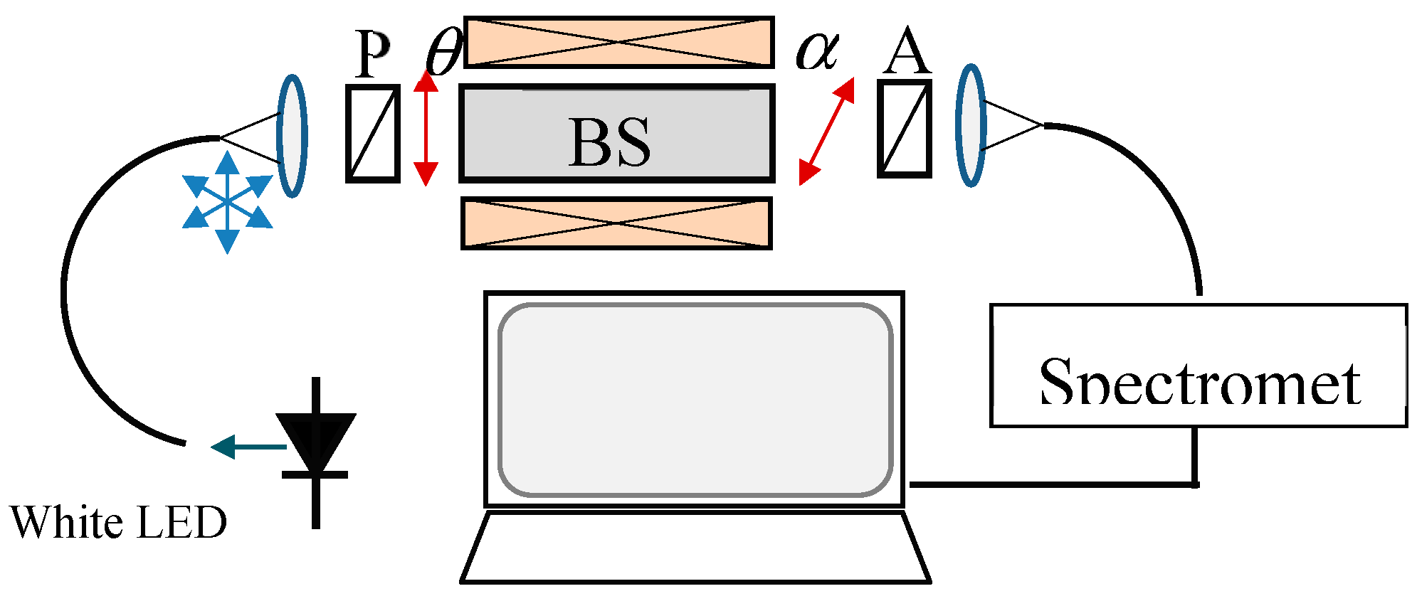
Figure 2.
Spectral response of the polarimetric sensor response: a) as analyzer angle increases from 0°C to 90°C; b) as current in the coil increases form -28A to +28A.
Figure 2.
Spectral response of the polarimetric sensor response: a) as analyzer angle increases from 0°C to 90°C; b) as current in the coil increases form -28A to +28A.
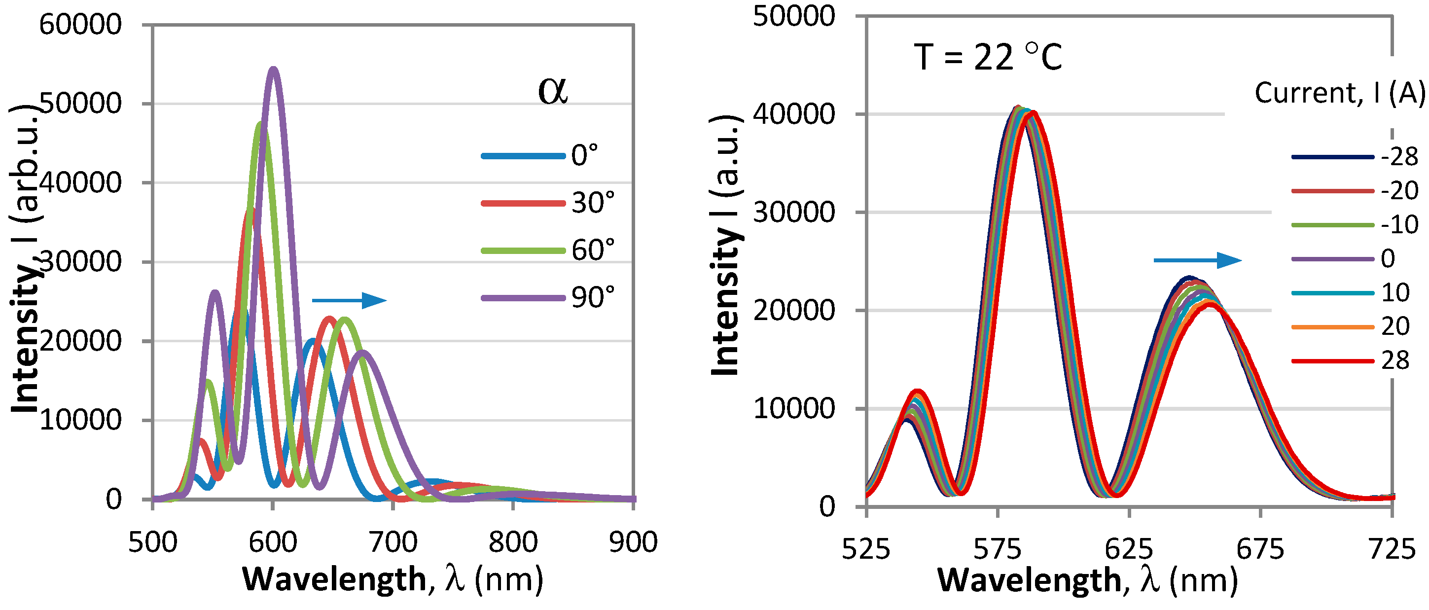
Figure 3.
Interrogation techniques: a) extrema wavelength shift; b) π-shifted differential shift.
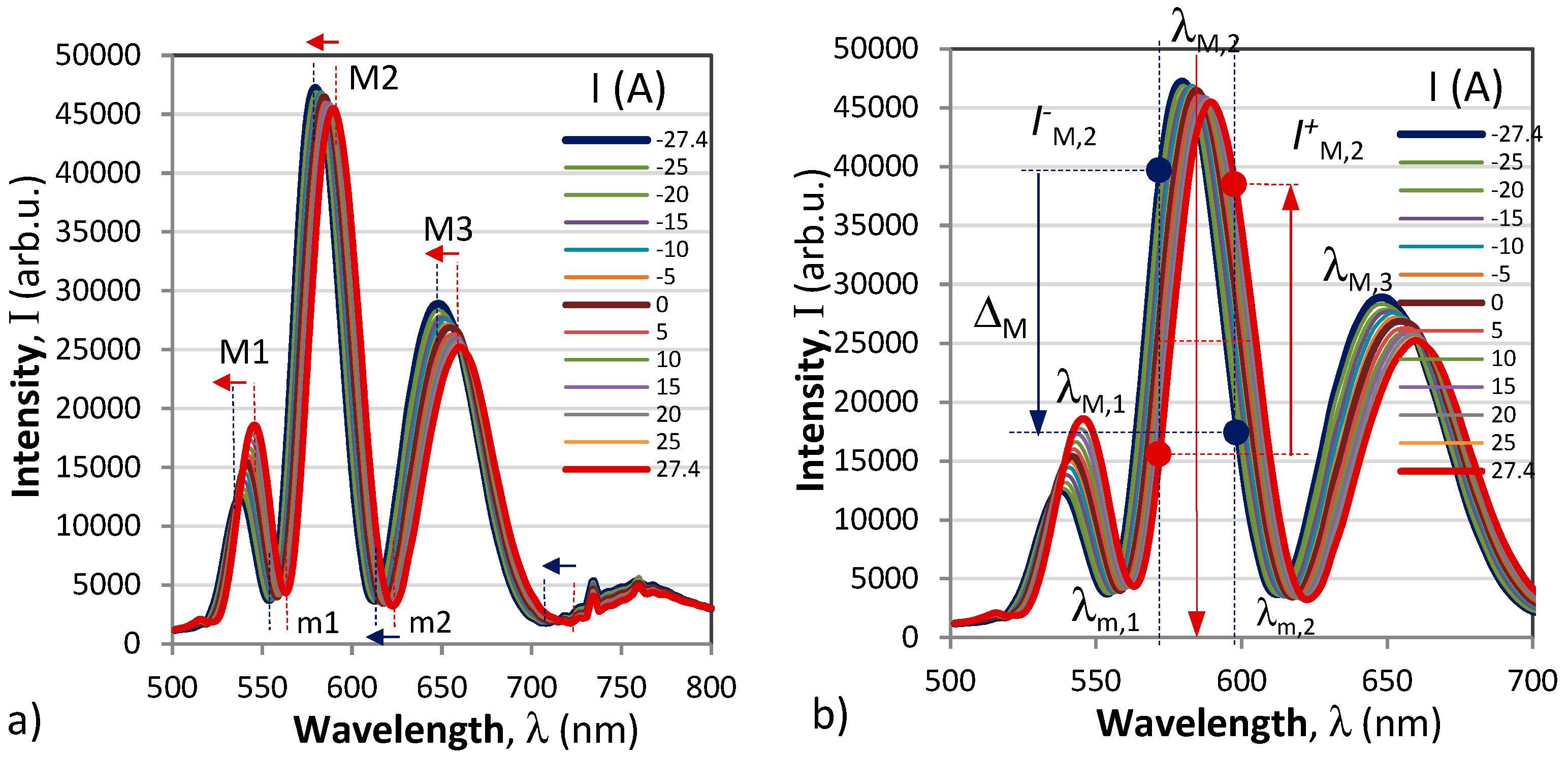
Figure 4.
Spectral responses of the extrema shift interrogation technique: a) wavelength shifts of the the maxima M1, M2, M3 and the minima m1 and m2, b) wavelength dependence of the sensitivities SI(λ).
Figure 4.
Spectral responses of the extrema shift interrogation technique: a) wavelength shifts of the the maxima M1, M2, M3 and the minima m1 and m2, b) wavelength dependence of the sensitivities SI(λ).
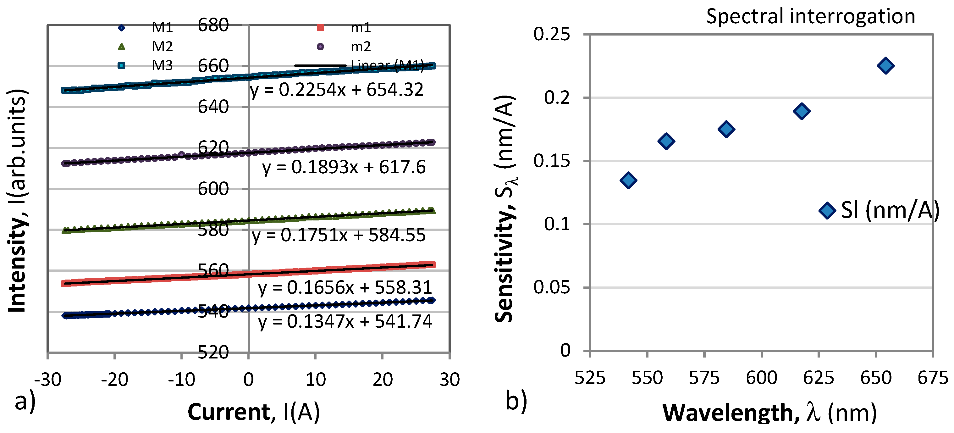
Figure 5.
Normalized differential responses of the π-shifted interrogation technique: a) wavelength shifts of the the maxima M1, M2, M3 and the minima m1 and m2, b) wavelength dependence of the sensitivities ΠI(λ) around maxima M2, M3 and minima m1 and m2.
Figure 5.
Normalized differential responses of the π-shifted interrogation technique: a) wavelength shifts of the the maxima M1, M2, M3 and the minima m1 and m2, b) wavelength dependence of the sensitivities ΠI(λ) around maxima M2, M3 and minima m1 and m2.
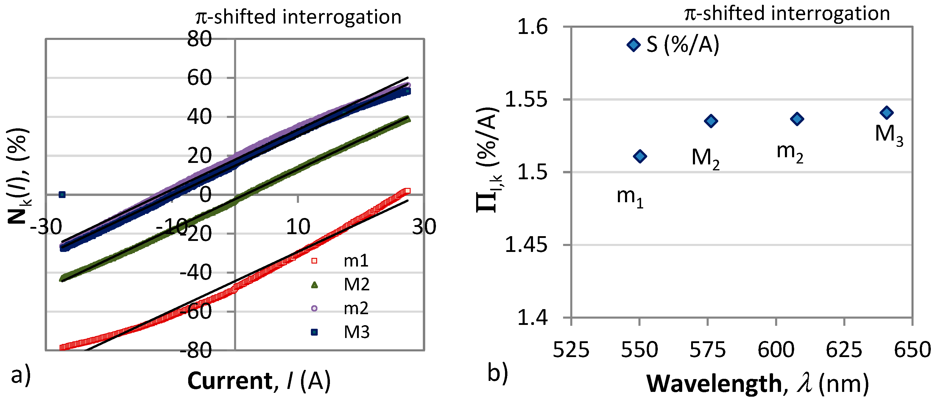
Figure 6.
Experimental set-up.
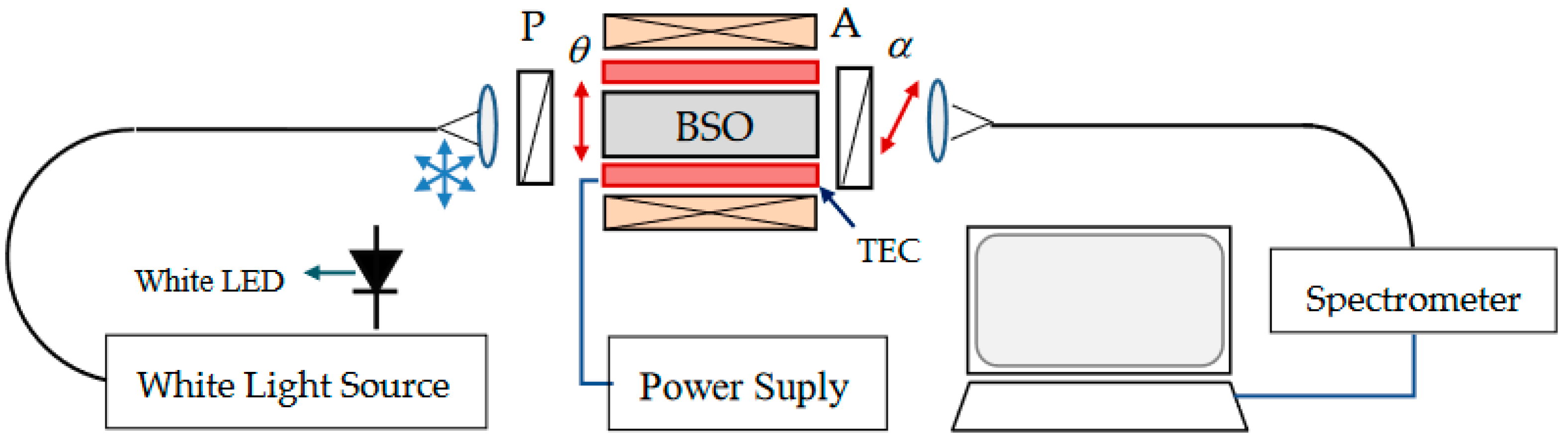
Figure 8.
Spectral and temperature dependence of the magneto-optical rotation without: a) V(λ)L; b) the maximum thermally induced variations over a 90°C temperature range.
Figure 8.
Spectral and temperature dependence of the magneto-optical rotation without: a) V(λ)L; b) the maximum thermally induced variations over a 90°C temperature range.
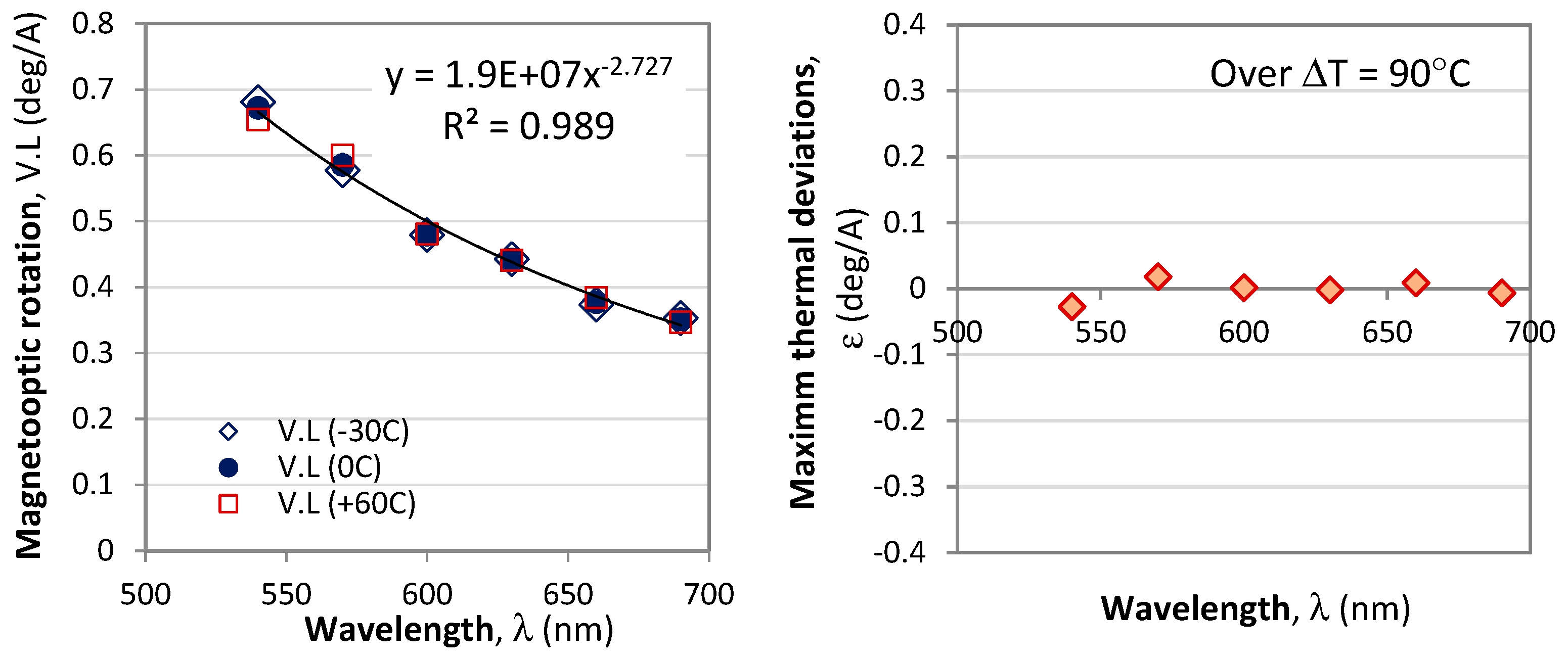
Figure 9.
Two responses of the polarimetric sensor for the analyzer turned at 0° and 90° given by the thin line. The thick line is a theoretical fitting to the response at 0° from (18).
Figure 9.
Two responses of the polarimetric sensor for the analyzer turned at 0° and 90° given by the thin line. The thick line is a theoretical fitting to the response at 0° from (18).
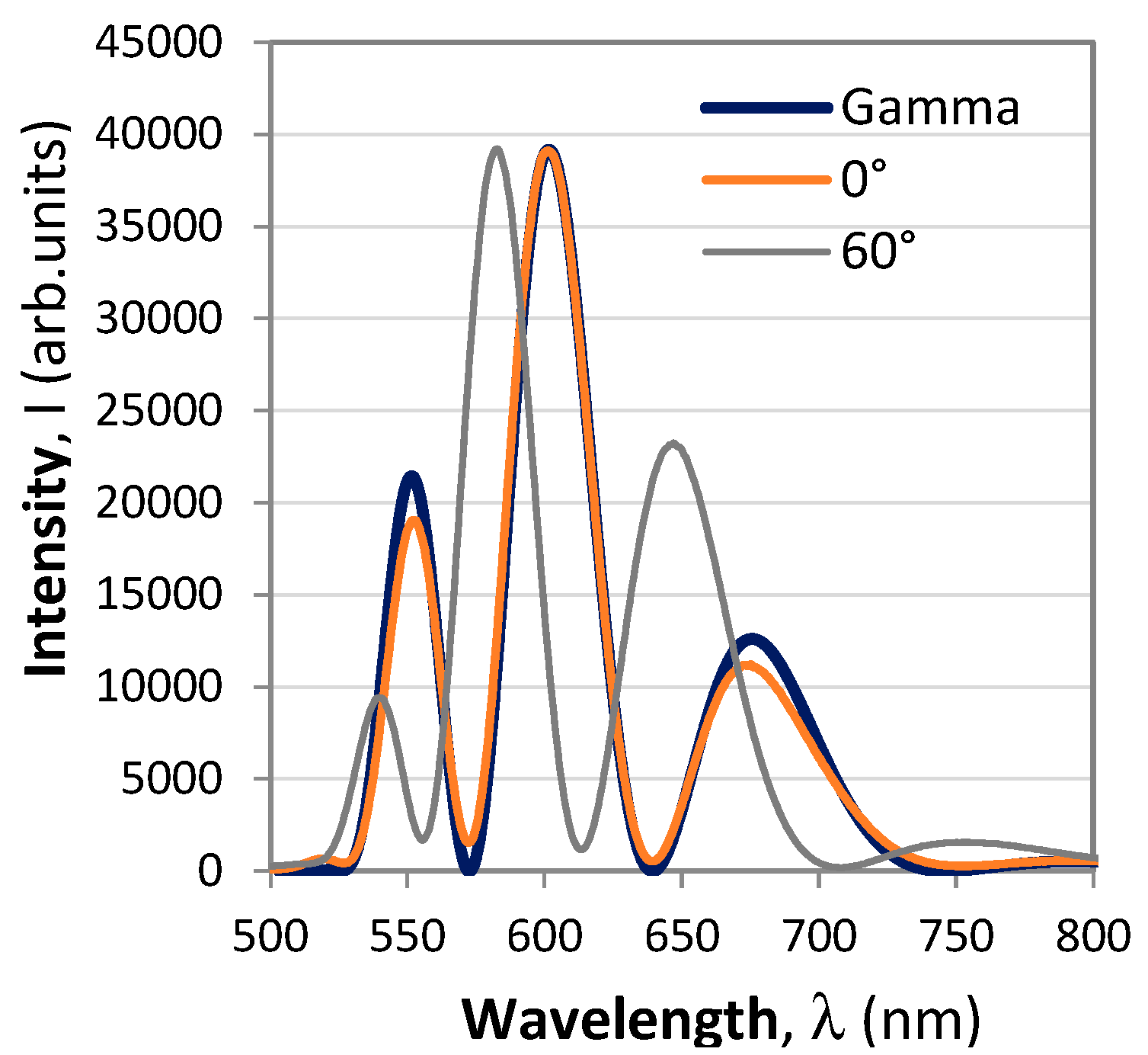
Figure 10.
Responses to current changes: s) shifts of the extremun wavelength vs. current changes from -100 A to 100 A; b) wavelength dependence of the sensitivity to current SI(λ); c) the temperature dependence of the coefficient A0(T) from (22a); d) the temperature coefficient A1(T).
Figure 10.
Responses to current changes: s) shifts of the extremun wavelength vs. current changes from -100 A to 100 A; b) wavelength dependence of the sensitivity to current SI(λ); c) the temperature dependence of the coefficient A0(T) from (22a); d) the temperature coefficient A1(T).
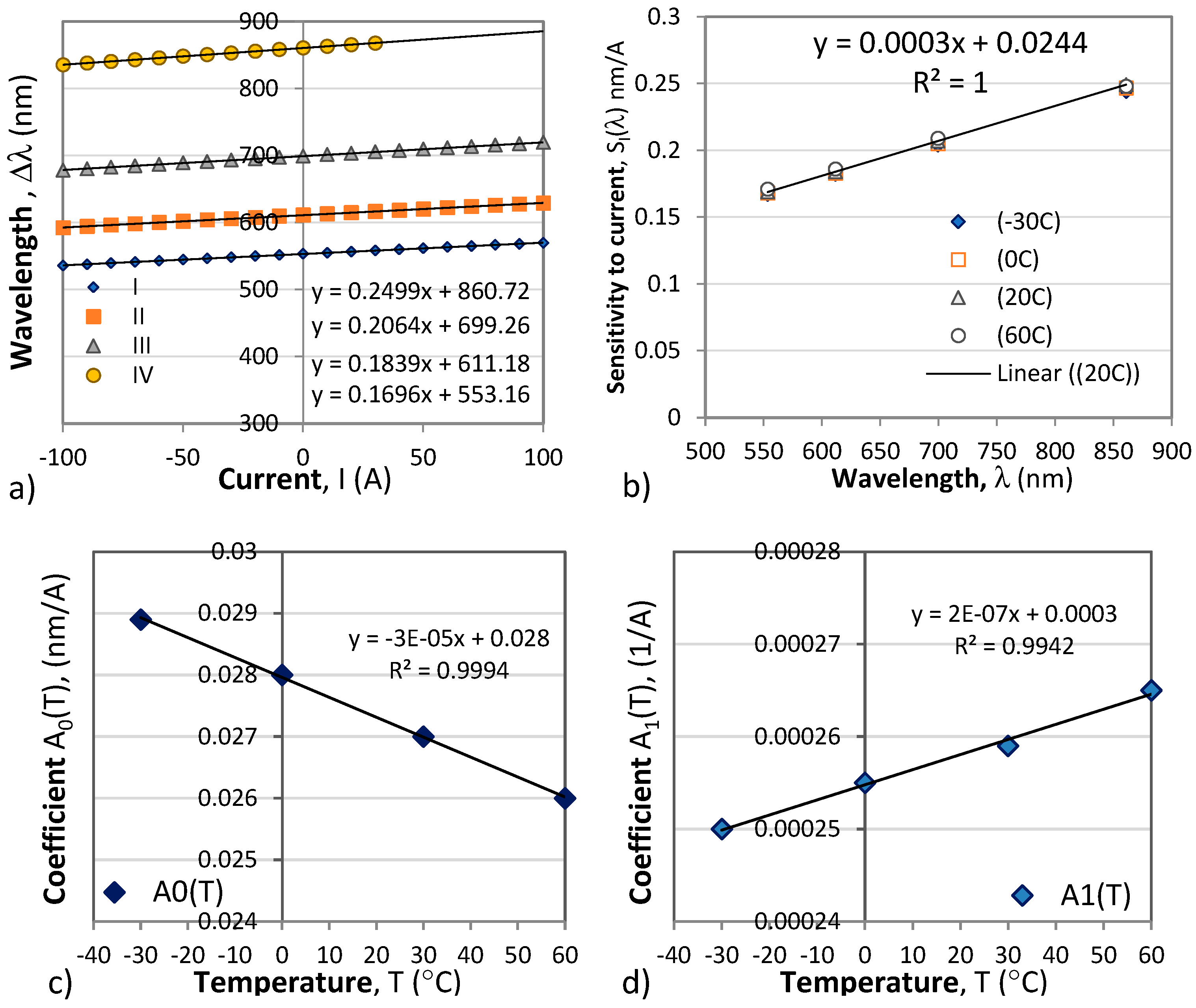
Figure 11.
Temperature dependence: a) Temperature induced wavelength shifts of four minima at I = 0A; b) Wavelength dependence of sensitivities to temperature ST(λ) for different currents; c) temperature dependence of the B0 coefficient from (23a); the thermal coefficient B1from (23).
Figure 11.
Temperature dependence: a) Temperature induced wavelength shifts of four minima at I = 0A; b) Wavelength dependence of sensitivities to temperature ST(λ) for different currents; c) temperature dependence of the B0 coefficient from (23a); the thermal coefficient B1from (23).
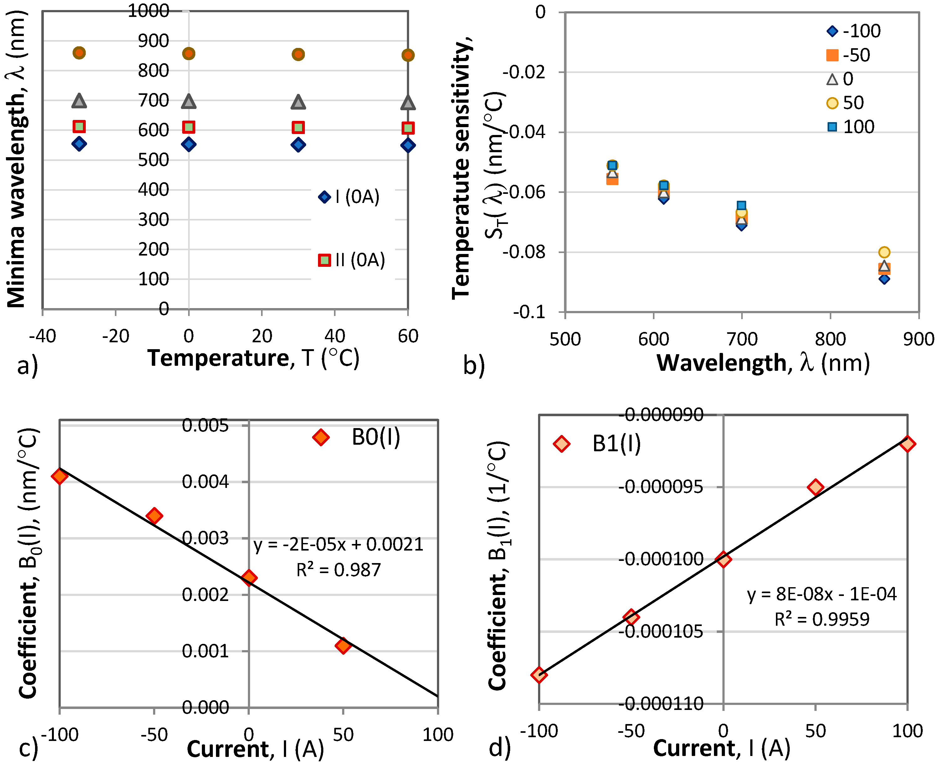
Figure 12.
Correspondence between calculated current and preset current: a) for the (λ1, λ3) pair; b) for the (λ2, λ3) pair.
Figure 12.
Correspondence between calculated current and preset current: a) for the (λ1, λ3) pair; b) for the (λ2, λ3) pair.
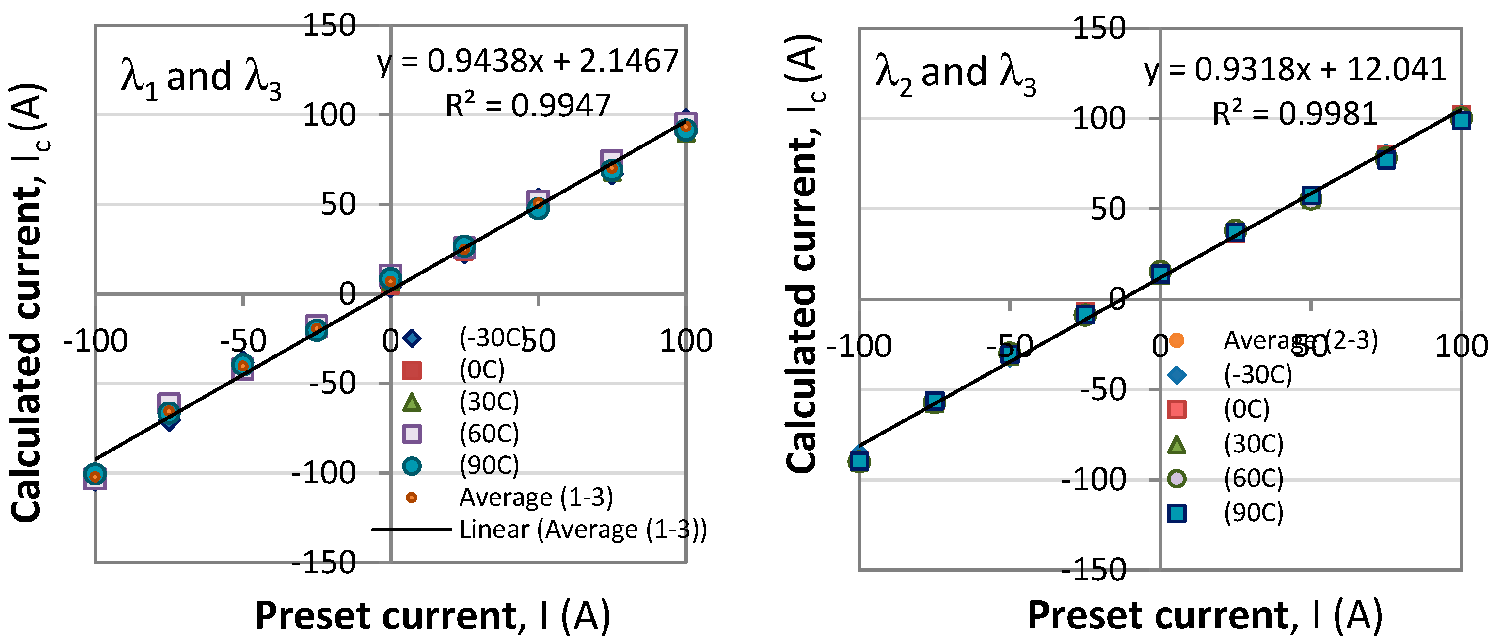
Figure 13.
Correspondence between calculated current and preset current: a) for the (λ1, λ3) pair; b) for the (λ2, λ3) pair.
Figure 13.
Correspondence between calculated current and preset current: a) for the (λ1, λ3) pair; b) for the (λ2, λ3) pair.
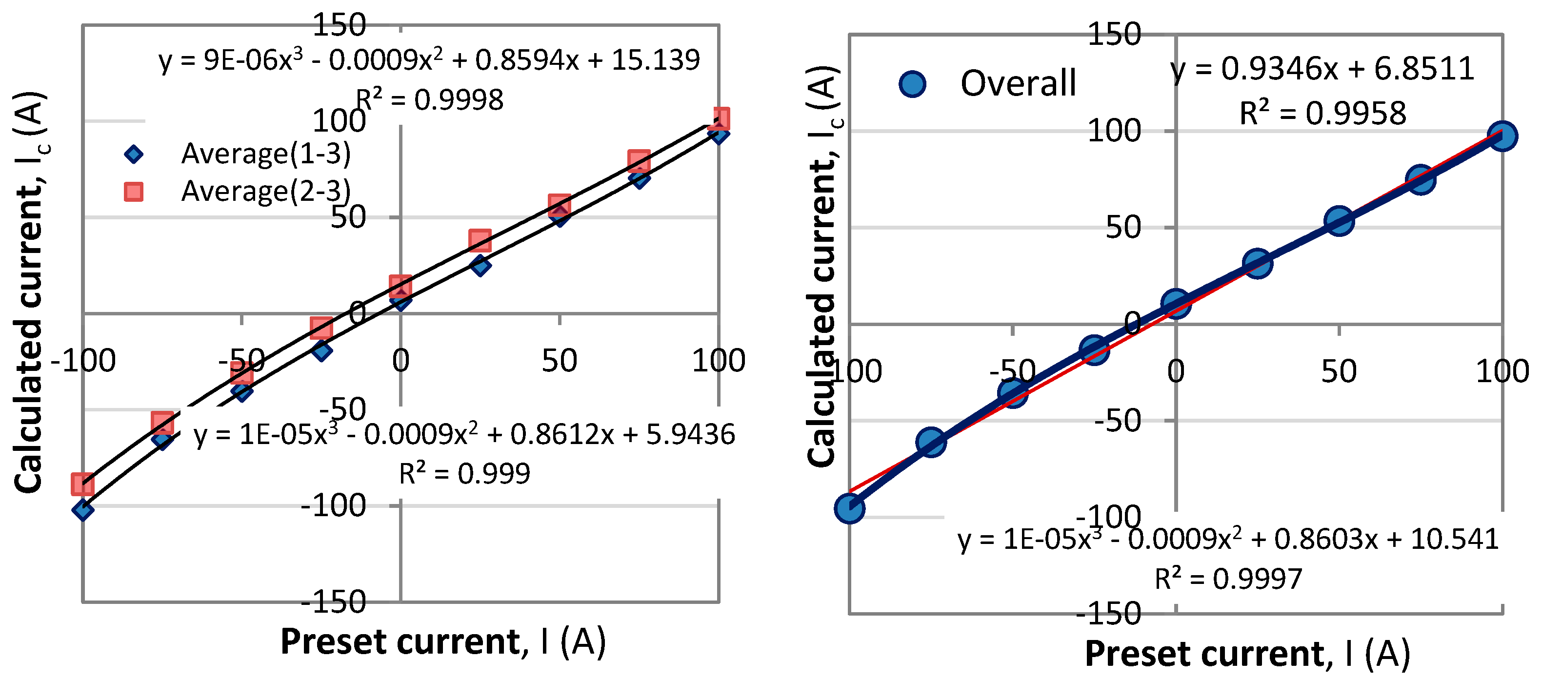
Table 1.
Coefficients for the expressions for the sensitivities SI and ST.
| A00 (nm/A) |
A01 (nm/°C/A) |
A10 (1/A) |
A11 (1/°C/A) |
B00 (nm/°C) |
B01 (nm/°C/A) |
B10 (1/°C) |
B11 (1/°C/A) |
| 2.8x10-02 | -3x10⁻⁵ | 2,548 x10-4 | 2x10⁻⁷ | 2.1 x10⁻³ | -2.05 x10⁻⁵ | -9.97 x10⁻⁵ | 8.2 x10⁻⁸ |
Disclaimer/Publisher’s Note: The statements, opinions and data contained in all publications are solely those of the individual author(s) and contributor(s) and not of MDPI and/or the editor(s). MDPI and/or the editor(s) disclaim responsibility for any injury to people or property resulting from any ideas, methods, instructions or products referred to in the content. |
© 2023 by the authors. Licensee MDPI, Basel, Switzerland. This article is an open access article distributed under the terms and conditions of the Creative Commons Attribution (CC BY) license (http://creativecommons.org/licenses/by/4.0/).
Copyright: This open access article is published under a Creative Commons CC BY 4.0 license, which permit the free download, distribution, and reuse, provided that the author and preprint are cited in any reuse.


