Submitted:
16 October 2023
Posted:
17 October 2023
You are already at the latest version
Abstract
Tropical cyclones (TC) are dangerous weather events and accurate monitoring and forecasting can provide significant early warning to reduce loss of life and property. However, the study of tropical cyclone intensity remains challenging, both in terms of theory and forecasting. ERA5 reanalysis is benchmark data set for tropical cyclone studies, yet the maximum wind speed error is very large (68 kts) and still 19 kts after simple linear correction even in the better sampled North Atlantic. Here, we develop an adaptive learning approach to correct the intensity in the ERA5 reanalysis, by optimising the inputs to overcome the problems because of the poor data quality and updating the features to improve the generalisability of the deep learning-based model. Specifically, we use TC knowledge to increase the representativeness of the inputs so that the general features can be learned with deep neural networks in the sample space, and then use domain adaptation to update the general features from the known domain with historical storms to the specific features for the unknown domain of new storms. This approach can reduce the error to only 6 kts which is within the uncertainty of the best track data in IBTrACS in the North Atlantic. The method may have wide applicability, such as extending it to the correction of intensity estimation from satellite imagery and intensity prediction from dynamical models.
Keywords:
tropical cyclones
; ERA5 reanalysis
; deep learning
; generalisability
; domain adaptation
1. Introduction
Tropical cyclones (TC) cause enormous damage around the world every year, especially in coastal areas [1,2,3]. Many scientists are contributing to find the regularity of tropical cyclone genesis, development and disappearance from the past to the present [4,5]. This regularity is also the cornerstone of forecasting techniques, for providing more accurate early warnings to protect people and property. Over the last century, observational technology, dynamical theory and forecasting have made great progress, but there are still many key problems to be solved. One example is the problem of tropical cyclone intensity. Especially the theory of intensity change is incomplete, intensity data are scarce, and intensity prediction is difficult [6,7].
Definitions of tropical cyclone intensity vary from agency to agency. Generally, it is defined as the maximum wind speed near the centre of the storm or the minimum pressure at the centre [8]. Agencies collect as many historical records as possible and then reanalyze them to provide a standard reference for researchers to use in the future. However, in-situ observations of tropical cyclones are very difficult to collect, so most of the data comes from satellite observations, with very little from aircraft reconnaissance [9,10,11]. The reanalysis of tropical cyclones is integrated into a well-known dataset known as the best track dataset. IBTrACS (The international best track archive for climate stewardship) is the typical one that collects global best track dataset and give the uncertainty estimation for intensity in maximum wind speed [12]. From 2004 to now, the uncertainty of intensity in the North Atlantic is 7 kts (knots), while in other basins it is 10 kts [13].
The best track data sets also provide a reference for the development of tropical cyclone monitoring and forecasting techniques. The Dvorak technique provides quantitative estimates of intensity in satellite imagery [14], so it is still widely used by operational agencies and the techniques have been updated several times [15,16]. For intensity prediction, the representative methods are the statistical model [12,17,18,19] and the dynamic forecasting model [20]. The former provides a fast and accurate forecast, while the latter is suitable for providing a more stable and long lead-time forecast. In most cases, they need to be combined to produce a more accurate forecast, such as statistical-dynamic model. With the advent of the artificial intelligence era in recent years, there are many new studies trying to explore different intelligent techniques to optimise or replace existing monitoring or forecasting techniques [21]. For example, they are using the convolutional neural network in image recognition to update the Dvorak technique [22,23,24,25,26], or non-linear deep neural networks to replace the traditional statistical model for intensity forecasting [27,28,29,30].
There may are two reasons why artificial intelligence methods can be widely used in tropical cyclone research. The first is that these kinds of data-driven methods are out of the existing physical theory, so they are expected to provide a new insight to find unknown knowledge. The second one is the strong representative ability of deep neural networks are shown as a powerful tool to fit a specific pattern hidden in the data, which is better than traditional methods such as linear regression to a large extent. However, these types of methods are highly dependent on the quality of the data. This means that it may be impossible to learn the correct knowledge or representation if the intelligent model is trained on poor-quality data. But in reality, it is also very difficult to evaluate the quality of data, especially tropical cyclones are a kind of suddenly changing weather phenomenon without complete and real observations.
Another problem is the model generalisability, deep neural network is verified with the strong representative ability, but the understanding ability is still questionable. It is because of the basic assumption of machine learning, the training dataset used to train the model and the testing dataset used to verify the model generalisability should be collected from the same data distribution, although they are individual [31,32]. This means that the sample size of the training dataset should be large enough, and the hidden information in the samples should be fully representative of the entire data space. So, the testing dataset can be a measure to test if the model is capable of understanding or strong generalisation. So far, the model trained on ImageNet dataset [33,34] may be close to the above assumptions. But in practical applications, such as tropical cyclones, the basic assumptions is far from achieving, because the learning task is largely limited by the sample size and value data without much noise. The emergence of transfer learning [35] provides a great opportunity to help solve the above problems [36]. There are studies in tropical cyclone research using transfer learning to improve intensity prediction [37].
In addition, the ERA5 reanalysis (ECMWF Reanalysis v5) provides an optimised estimate of the current atmospheric state, which provides a detailed description for tropical cyclones [38]. It may not be the most accurate representation of tropical cyclone intensity compared to satellite imagery or in-situ observations, but it contains additional environmental information that may be an effective supplement for tropical cyclone monitoring and forecasting [39,40,41]. And the data format is similar to the output of dynamical models, so it can be the replaced dataset to develop new methods for the latter applications. There are some studies to explore the capability of tropical cyclone representations in ERA5 reanalysis [42,43,44].
Therefore, we aim to correct the intensity in the ERA5 reanalysis using the value in IBTrACS as a reference. There are some related works to correct the intensity in operational forecasting [45,46,47]. Differently, we develop an adaptive learning approach based on deep neural networks and transfer learning methods to solve the problems of data quality and weak model generalisation. The experiments in the North Atlantic verify the effectiveness of our approach. It can be easily extended to other learning tasks using new data. Furthermore, it is not restricted to the same computation platform, deep learning framework or python version, which can be easily extensible by other users.
The paper is organised as follows: the introduction gives a brief description of the background, related works and our work. The Methodology presents the learning tasks, the concept of our approach, and the basic knowledge and experimental setup for implementing this approach. The Results section shows the preliminary data evaluation and analysis of the experimental dataset, and how to optimise the results from the baseline using our approach. We also express the our attempts, unsolved problems and future plan in the section of Discussion. Finally, we summarize the whole work, progress and potential in the Conclusion section.
2. Methodology
2.1. Our approach
Our learning tasks can be defined as follows:
which means that our goal is to find the optimal F with strong generalisability. X is the inputs, Y is the outputs, and is the mapping from inputs to outputs. Considering that the correspondence between X and Y in data space may not be clear, the difficulty of learning F increases.
Therefore, we develop an adaptive approach to learn it well, which can be divided into three steps, gradually or individually. The first is to learn the mapping F from X to Y directly. If this works, the goal is achieved. The second is to update the inputs in and then learn the mapping F from to Y. Here we define . And is the feature extractor from inputs to feature , and is the mapping from feature to outputs Y. If it doesn’t work, we go to the next step to update the to or update the general feature to as the specific features until the goal is achieved. So now or . In this step, is the feature mapping from to and is the new mapping from the updated feature to Y. Actually, each path from X or to Y shown in the Figure 1 below is available and can be chosen in different learning tasks if it works. However, here we only present three ways that were used in our experiments, and they can be formulated as follows:
2.2. Brief introduction
2.2.1. Data
In this paper, Y is the intensity label from the best track dataset - IBTrACS. It provides the storm centre, time and other attributes we need and is widely used as a reference to research various tropical cyclone techniques. The data from the US agencies is usually of the highest quality. The Table 1 shown in below present the basic information of the tropical cyclone records collected from IBTrACS technical report.
X is the inputs, and it is the ERA5 reanalysis. ERA5 provides the global atmospheric state with a latency of about 5 days and is avaliable from 1940 to present. The spatial resolution is 0.25 and the temporal resolution is one hour. In addition, they are homogeneous and consistent gridded dataset with a large number of atmospheric, ocean-wave and land-surface quantities. The Table 2 shown in below present the basic information of the ERA5 data from the official website.
2.2.2. Deep neural networks
Considering the strong representativeness, we use deep neural networks to learn F. It starts from MLP (Multilayer Perceptron) with nonlinear activation function, which can be effectively used to fit the nonlinear mapping or function. It is assumed that given enough data, the network can be used to estimate any function. After that, CNN (Convolutional Neural Network) seems to be used in image classification by extracting the spatial features of the image, and it achieves great success now. It can also reduce the parameters of networks by sharing parameters in the receptive field. However, the deeper the network, the more obvious the problems of gradient disappear. ResNet [48] is designed to use short-cut way to solve the problem of gradient disappear, while it can maintain the strong representative ability. It has been widely used in computer vision and it is also the basic stone in many industrial applications. The core module of ResNet is the residual block. Here, We only use the simplest version that is ResNet-18. Given the inputs, after the feature extraction of resiudal blocks with convolutional layers, there is an average pooling layer to reduce the dimensionality of features to 512, and then the features are converted to output layer to finish our task.
2.2.3. Transfer learning
Because of the problems mentioned in the introduction, transfer learning is a good way to improve the generalisability of the model. The simplest method is fine-tune, which can be used to help the trained model adapt to new samples. Although it is able to retrain the model to improve the accuracy in a fast way, it still does not solve the problems of different data distribution between the training and testing dataset. Therefore, domain adaptation (DA) is also used in this paper. It is designed to help a model trained in the soured domain adapt to an unknown target domain, which is similar to our problems. The core idea of domain adaptation is to find the similarity of two domains and try to reduce the distance between two datasets defined by the general distance function. And MMD (Maximum Mean Discrepancy) is one of the most popular metrics in transfer learning, especially in domain adaptation. Furthermore, one of the key problems is to define a new loss function that adds the distance between the source and target domains.
2.3. Experimental setting
2.3.1. Dataset
In order to carry out experiments, we first need to prepare the dataset. The samples we select from follow the rule as follows:
- Data are post reanalyzed by agencies, and it means that ’TRACK_TYPE’ is flagged as ’main’;
- Only tropical cyclones (’NATURE’ is marked as ’TS’) analyzed and Saffir-Simpson Hurricane Scale (SSHS, US agencies) is larger than 0;
- Records from 2004 to 2022 and only in North Atlantic, and they are provided by US agencies.
Therefore, the description of the samples can be found in the Table 3. After that, we download the corresponding ERA5 data with each sample using the Python API to adjust the variables, levels, region size, etc. In particular, we follow our previous work in 2019 [49] to select the following variables. They are described as follows:
- Variables: u (u-component of wind), v (v-component of wind), t (temperature), r (relative humidity), h (geopotential) at pressure levels and sst (sea surface temperature) at surface;
-
Pressure levels: 1000 hPa/925 hPa/900 hPa/800 hPa/700 hPa/600 hPa/500 hPa/400 hPa/300 hPa/200 hPa/100 hPa.
The experimental dataset consists wind that is calculated by u and v. Then we need to split the dataset to train the model, select the model and evaluate the model. And they are training dataset, validation dataset and testing dataset separately. There are several splitting methods in machine learning, such as hold-out with stratified sampling, cross-validation and bootstrapping [32]. These splitting methods are based on a basic assumption, which is to ensure that the training and testing dataset are drawn from the same distribution. However, the testing dataset can only be used to test whether the model is learning the knowledge from the sample space. For our research problem of intensity correction, we need to apply the trained model in the real scene. Therefore, we split the dataset according to the consecutive years. We try to use the new storms to test the generalisability of the model trained on the historical storms. Therefore, we adopt three splitting methods. The first one is to use the leave-out in machine learning, we use 80% for training, 10% for validation and 10% for testing. The second one is to use the 2021-2022 samples as testing dataset, and the rest is split into training and validation dataset. The third one is to divide the data strictly according to the years. So we use the samples from 2004-2018 to train, 2019-2020 to validate and 2021-2022 to test the model.
2.3.2. Objective function
The objective function of the whole training process we use here is the mean square error, and the formula is defined as follows:
N is the size of the samples, is the label of the i th label, and is the i th output value of the networks.
2.3.3. Evaluation metrics
The metrics we choose here are bias and root mean square error (RMSE). The former is used to evaluate the accuracy of the model, and the latter is used to evaluate the variability of the model. They are formulated as:
Also N is the size of the samples, is the label of the i th label, and is the i th output value of the networks.
We perform all comparative experiments using the same computational environment. The module we use in this paper is Python 3.8, Keras 2.8.0, Tensorflow 2.8.0, Scikit-learn 1.3.0, Numpy 1.24.4, Pandas 2.0.3, MetPy 1.5.1 and so on. We also use the TESLA-V100 GPU to improve the computational efficiency. We set all random seeds in the experiments to 42 to reduce the noise of randomness.
3. Results
3.1. Data analysis
3.1.1. Overall information
To evaluate the hidden correlation in the original dataset, we analyse them using statistical methods. Unlike experimental dataset such as ImageNet in image classification, the relationship between inputs and outputs is certain and obvious. Our dataset contain the samples recorded in IBTrACS, only some samples are filtered according to our specific task in tropical cyclones, not for machine learning. Therefore, the correspondence between inputs and outputs still needs to be explored.
One of the definitions of intensity is the maximum 10m wind speed over the surface near the storm centre, so we can calculate it using ERA5 reanalysis. We call the intensity in the reanalysis ERA5_Vmax, and the intensity in the best track dataset IBTrACS_Vmax. The total bias of the whole dataset of 4145 samples is -43.08 kts and the RMSE is 47.41 kts. The scatter plot in the Figure 2 describes the correlation between ERA5_Vmax and IBTrACS_Vmax. We can see that there is no obvious linear correlation between these two variables as the value of the linear fit with 95% confidence is 0.16. It is noticeable that there are obvious one-to-many and many-to-one relationships between ERA_Vmax and IBTrACS_Vmax. For example, the Vmax in IBTrACS is 100 kts, but the possible values in ERA range from about 22 kts to 70 kts.
We also plot the cumulative curve of the RMSE as shown in Figure 3 and we find that the minimum error is close to 20 kts and the maximum error is approximately to 90 kts. The error distribution is comparatively balanced in different range, and the RMSE of nearly 80% samples is less than 55 kts.
3.1.2. Error analysis
To analyse the factors related to the error distribution, we divide the RMSE of all samples into different groups. Here we only consider the different years and categories. From Figure 4 (a) we can see the variation from 2004 to 2022, but there is no obvious trend with the years, whatever for the bias or the RMSE. During these years, the average RMSE is the minimum in 2006 with about 30 kts, while it increases to the maximum in 2007 with about 70 kts. The RMSE of the remaining years fluctuates with an average value of about 40 kts. From Figure 4 (b) we can observe an obvious increasing trend in the errors as the category grows. The average RMSE of the Category 1 samples is about 30 kts, but 90 kts for the Category 5 samples. This means that the average Vmax of different categories in the ERA reanalysis makes a small difference.
3.1.3. Storms correspondence
Apart from the overall errors in the whole dataset, we all try to check the correspondence between the storms contained in ERA5 and IBTrACS. We use the LMI (Life Maximum Intensity) to represent the storm characteristics. We plot the scatter plot in Figure to describe the relationship between the LMI of storms in IBTrACS (IBTrACS_LMI) and storms in ERA5 (ERA5_LMI). It shows an increasing trend as the number of categories increases. Here, the category indicates the type of storm, not the samples. For example, the Category 3 storms show that the LMI of this type of storm is in the range of Category 3 with an SSHS (Saffir-Simpson Hurricane Scale) of (96 ≤ W < 113). And there are 20 Category 3 storms in this dataset.
We also rank the storms by LMI in ERA and IBTrACS and calculate the overlap rate in different categories. We can see that the rate of the top 10% is 0.5 only in Category 3 storms, and the rest is 0. As for other categories, such as Category 1 and Category 5, they all show a weak correlation. The overlap rate of the top 50% is only 0.57 for Category 5 storms.
3.2. Our adaptive approach
3.2.1. Baseline
After a preliminary evaluation of the hidden correlation between the intensity value in ERA5 and IBTrACS. We start to use our approach to correct the intensity in ERA5 to be close to the intensity in IBTrACS. To verify the effectiveness of the methods used, we need to split the testing dataset to evaluate them. We present three methods in the methodology and compare the distributions of the outputs (labels) in Figure 6. If we apply the first method, we can see that the distribution of training, validation and test is very similar. And in the second method, the distribution of training and validation is similar but different from the test data set. As for the third method, the validation and test are all different from the training dataset.
In fact, there are only two testing datasets. One is randomly split and the other is split by consecutive years. The bias and RMSE from point to point in the Table 5 show the errors in the ERA5 reanalysis. If we calculate the Vmax using the 10m wind speed in the surface layer, we can see that the RMSE is 69.82 kts in the testing dataset (10%) and 67.98 kts in the testing dataset (2021-2022) before correction. After linear correction, the RMSE is reduced to 20.86 kts and 19.01 kts respectively. The bias of these two datasets are all close to 1 kts, confirming the accuracy of the linear model. And there are few differences between the results of the two testing datasets. We also use the wind speed at the 850 hPa pressure level as the inputs and get similar results. The linear method corrects the bias and RMSE significantly. The wind speed at 850 hPa is collected from the ERA5 pressure level and not from the surface layer, so it may contain less noise. We also compare the wind structure in these two levels shown in the figure, we can see that the pattern of 850 hPa is more obvious than the surface. We therefore choose the 850 hPa as the base level for constructing the inputs.
The above methods show the potential of linear correction. But it remains a large RMSE when used for applications. So we consider using non-linear methods to further correct it. Deep neural networks are our first choice, which we introduce in the previous parts, and ResNet-18 is used as our basic network architecture. We split the dataset into the three ways mentioned above and then use the wind speed at these two levels to train, validate and test the network. We use bilinear interpolation to change the inputs shape to (None, 224, 224, 1) to match the original inputs shape of ResNet-18. We also change the unit of the output layer to 1 for our regression task. We set the loss function to mean square error (MSE) and select the Adam (Adaptive moment estimation) algorithm as the optimal algorithm. For the Hype parameters, we set the batch size to 32, the epochs to 50, and the learning rate to 0.0001.
The results are very similar between the surface and 850 hPa, which also validates our operation of using 850 hPa as a replacement for the base level. We focus here on the bias and RMSE of 850 hPa as an input. They show significantly different results when splitting the testing dataset in Table 6. The test RMSE is 9.8 kts when taken from the same data distribution with the training dataset using the randomly split methods. But it shows that the RMSE is all above 16 kts even using different validation split methods when the testing dataset is from the following years. The scatter plot in Figure 8 (a) shows an almost linear correlation between IBTrACS_Vmax and ResNet_Vmax in the testing dataset, so it is possible to use linear correction to remove the residuals. However, there is no obvious correlation in the testing dataset (2021-2022). We can find an improvement using the non-linear model that is ResNet-18 than the linear model in intensity correction, but it is still far from the allowed error of intensity in operational application.
In conclusion, we set the 850 hPa as the baseline level as the inputs, and ResNet-18 is the baseline model in our experiments. And the bias of -2.28 kts and RMSE of 16.41 kts testing dataset (2021-2022) is the baseline of network model in this paper. Therefore, we still use our approach to optimise the results.
3.2.2. TC knowledge for optimising the inputs
As machine learning approaches rely strongly on data quality, we find that there is no obvious correspondence of a single surface layer using statistical methods. To further validate this conclusion, we update the inputs in three ways as shown in the Figure 9. The first is to use the original data without bilinear interpolation to preserve the true information hidden in the data. The second is to crop the region into and then use bilinear interpolation to resize it. The reason for using the crop operation is to make the structure of the wind near the storm centre clearer. And the third operation is to rotate the inputs according to the direction of the storm speed to unify and standardise the wind pattern, and then crop and resize it. From Table 7, we can check the effectiveness of resizing the inputs compared to the result of the original inputs. Another finding is that crop makes a little improvement, but rotate operation is not useful. Therefore, in the next experiments we will only use the crop operation.
The above experiments may provide new evidence that the single-level correspondence is ambiguous, and that the one-to-many and many-to-one problems remain to be solved. So we add additional information to the inputs, trying to ensure that the inputs contain enough information that can be learned by the neural networks. We do this in two ways, to increase the spatial information of the wind and then to increase the variable information. Here we use the base level of 850 hPa and add the middle level which is 500 hPa and the top level which is 200 hPa. We add the equivalent potential temperature that contributes to the TC evolution calculated by MetPy using pressure (p), temperature (t) and relative humidity (r). We find the effectiveness of this operation in Table 8, and the RMSE is reduced to 14.90 kts when we use the variable of wind and in three levels.
3.2.3. Adaptive feature learning for improving generalisability
Although the results are now better than the baseline after updating the inputs, the generalisation of the model does not seem to improve much. So in this section we start to change the way we find solutions. We split the model from inputs to outputs into two parts and update them separately. In particular, we focus on considering whether the inputs-feature and feature-output mapping is effective or not. We first mention three ways of splitting the dataset. And then we find that the results of the testing dataset from the randomly split are satisfactory, but the results of the testing dataset from the subsequent newly coming years in the Table 6 are not satisfactory. We can conclude from the former finding that the ResNet network is able to represent the inputs with effective general feature in the whole data space. However, in the sub-data space of the testing dataset from the subsequent newly coming years, the general feature extractor of ResNet-18 in the training dataset from the previous years is not sufficiently effective for the changing data distribution. As for the reasons, one of them may be that the mapping from feature to outputs is not accurate enough, and another reason may be that the general feature from the training dataset needed to be adapted as the specific feature in the new sub-data space in the testing dataset.
We perform the following experiments to validate the above assumptions. The first operation is to enlarge the training dataset using data augmentation to reduce the overfitting and then improve the generalisation of the feature. It also helps to reduce the impact of sample size and validate the small size can also be used to train a network model. Specifically, we use the random rotation to increase it, since we have a finding in Table 7 verify that there is no obvious impact on the results when rotate the inputs. We use the same experimental setup as in the previous experiments, including the computational environment, network architecture and hype parameters, and so on. We just increase the epochs to 100 and save the best model in the training process. And we found that there is not much difference between different sample sizes. To balance the computation and generalisation, we use the model trained on the third experiment shown in the Table 9 for the next experiments.
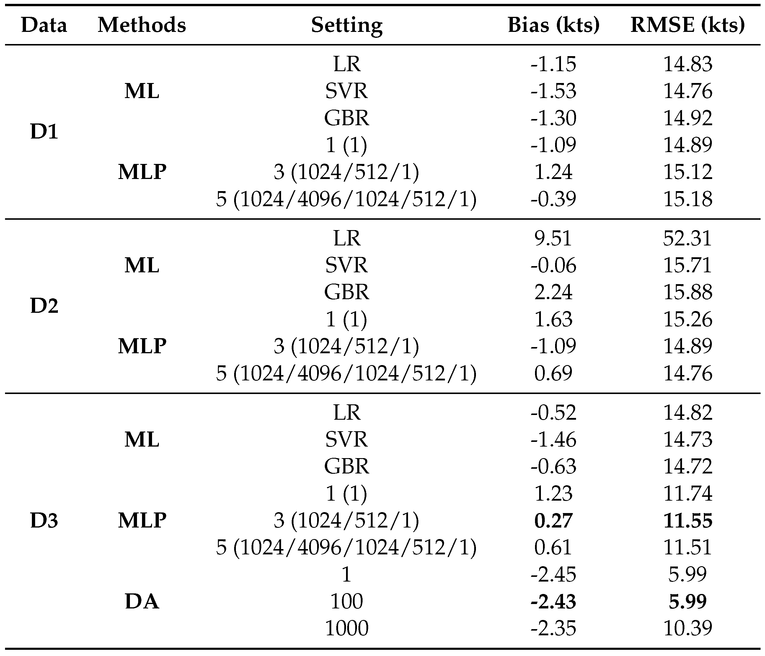
We fix the general feature extractor from the model trained in the last experiments. Now we need to reorganise the dataset. We can get the feature from the training dataset (2004-2018) named , the validation dataset (2019-2020) named , and the testing dataset (2021-2022) named . In the first set of experiments, the feature or feature-output mapping is updated using the original data information in the previous training dataset. The dataset used to retrain a model is D1 shown in the Table 10, and the method we use here are classical ML (Machine Learning) algorithms and MLP (Multi-Layer Perception). The top-3 algorithms in our validation is LR (Logistic regression), SVR (Support Vector Machine) and GBR (Gradient boosting regression). The choices of MLP are a single layer with one unit, or three layers with units of 1024, 512, 1, or five layers with units of 1024, 4096, 1024, 512, 1. The second group of experiments is used to update the feature or mapping using the data information in the previous validation dataset, to check the effectiveness of local information that may be similar to the testing dataset. The dataset is D2 and the methods are the same as the first group. The third group of experiments is to update the features and mapping using all available data information, including the previous training and validation dataset. The dataset used in this experiment is D3, and we add the domain adaptation (DA) except for the above methods. We set the loss weight of MMD (Maximum Mean Discrepancy) to 1, 100 and 1000 separate. In all experiments, the inputs in are , and the outputs are . It is the same with the inputs and outputs in (, ) and (, ).
As we mentioned in the methodology, there may be some differences in the data distribution between the training and testing dataset. Therefore, we refer to the idea of domain adaptation, and we can consider as the source domain and as the target domain. And the architecture design is the source of DaNN (Domain Adaptive Neural Network) [50] and DDC (Deep Domain Confusion) [51]. Our loss here is calculated from two parts. One is the MSE between the prediction and label in the testing dataset, and the other is the MMD distance between the feature of the training and test data. The process is shown in Figure 10 and the total loss can be expressed as
In this formula, demostrates MSE and demostrates the square of MMD. In details, the square of MMD can be expressed as follows:
is the mapping to transfer the original data into the RKHS space (Reproducing Kernel Hilbert Space), and , are the sample sizes of the training and testing dataset separately. So that the features can be compared in high dimension. And here we use the multiple-kernel MMD (MK-MMD). In addition, one of the key issues is to find the appropriate weight to balance the two parts of the loss. We try to make the feature of the test close the feature of the train and update the mapping from feature to outputs. And the aim is to make the general features from the training dataset fit in the testing dataset, so that they can be used to improve generalisability.
The results show that there is not much improvement in the RMSE using D1 and D2, whether the feature and feature-output mapping are updated or just the feature-output mapping. But there is an obvious progress when using D3. Actually, when using MLP with one unit, it only updates the feature-output mapping. But when we use three layers including 1024, 512 and 1 units, the feature has been updated to the new one, but the shape is still (None, 512), and the same with new feature-outputs mapping. The results show that three layers is between than one layer and five layers, and it reduce the RMSE to 11.55 kts. So we can try to add the information of test data to optimise the new feature to consider if there is further improvement. We use the network shown in Figure, and adjust the loss weight of MMD in different quantities. And we find that the results are not much different in the range of [1, 100], and it reduces the RMSE to 5.99 kts. But the RMSE increases when we increase the weight to 1000. Therefore, we analyse the prediction of the second experiment with domain fitting methods. The error distribution in the Figure 11 shows that the error was centred in the range [-20, 20] and others are outside this range. As for the distribution of the predictions, it still shows a Gaussian distribution, which does not fit the distribution of the outputs. The reason for this is that we use MSE as the main loss function, it does not change even if we add the mmd loss.
4. Discussion
As we show in the previous introduction and experiments, the intensity errors in the reanalysis dataset are large and need to be corrected. Traditional linear correction can reduce the errors to some extent, but some problems remain in practical operation. This may be because there is no obvious linear correlation between the intensity value calculated from reanalysis and the true value in the best track dataset. So here we use non-linear methods to try to improve it. Since ResNet is a widely used network with strong representativeness and solves the problem of gradient disappearance in deep neural networks with residual block, we use it to train the base model and then set the baseline. However, when we split the dataset in different ways, we find that there are many differences, especially in the selection of the testing dataset. If we use the method in machine learning to randomly split the testing dataset with a ratio like 10%, we can get a satisfactory result. But if we based on the requirement of practical tropical cyclone correction to split the testing dataset with consecutive new coming years, the result is not satisfactory. We consider that the former may follow the basic assumption that the training and testing dataset are from the same data distribution, but the latter obey it. It also means that the correspondence between inputs and outputs may change over time.
To solve this problem, our first option is to optimise the inputs. Since the outputs (labels) are fixed, the inputs contain more value information, making it easier to learn the correspondence for networks. Undoubtedly, the methods to update the inputs are based on existing tropical cyclone knowledge and then combined with general data processing methods in machine learning. For example, we crop the inputs to half their original size to make the central pattern clearer. We also rotate the inputs with the direction of the storm to unify the wind patterns going forward in the same direction and reduce external noise. But it seems that the crop operation is a bit useful here and the rotate operation is not. So for the next experiments we can crop the inputs to optimise the results. We also randomly rotate the inputs to increase the training dataset to reduce overfitting and improve the generalisability of the features. In addition, we increase the spatial levels of the wind to include bottom, middle and top information of tropical cyclones, and add the physical variable related to tropical cyclone development to the inputs. The results also show positive feedback, so we use the inputs with more variables and levels as the optimised inputs for the next parts. However, although the overall performance has been greatly improved compared to linear correction and the basic version of ResNet with the simplest inputs of 850 hPa. It seems that the problem of different data distribution in the training and testing dataset is still not solved, so the trained model may have weak generalisability.
Fortunately, transfer learning is designed to solve the problem of different data distribution, so it provides a new insight to help solve our problem. So we start to update the feature extracted from the trained model and the mapping of feature outputs using the idea of fine-tune and domain adaptation. We try to update these two parts using the original training dataset, but it does not work for the testing dataset. So then we update these two parts using the local information in the original validation dataset that is different from the training dataset, but it still does not work. Also, we update these two parts using all available information in original training and validation dataset, we find an improvement with the test result. Finally, we use the features of the original testing dataset to participate in the new training process for updating the features and feature-output mapping. The results show a significant decrease with the test errors, and now the RMSE of intensity is within the uncertainty of the North Atlantic. This means that it can hopefully be used in practical applications and provide a relatively accurate correction for intensity.
However, there are still many problems to be solved and assumptions to be validated for our work. Firstly, we only use in the tropical cyclone data in the North Atlantic from 2004 to 2022, the reason why we choose is it is of the highest quality to train the network model. However, if our approach is applied to other basins or historical years, with the best track data is inhomogeneous and noisy, there may appear new problems. Therefore, the approach still needs to be validated for other datasets to make it general and practical. Secondly, we only use ResNet-18 as the feature extractor in this paper, maybe there are better choices like ResNet-34, 101, other general network architectures like Xception or custom networks and so on. And the basic loss function, we only use MSE, maybe there are more appropriate objective functions for the specific tasks. All the parts of deep learning in this paper is the basic setting, and it can be optimised in many ways. Here we aim to provide the baseline version. Thirdly, the setting of the final domain adaptation methods still needs to be validated and explored. Although the method helps us to achieve the goal, it still lacks some explanations to a large extent. For example, does it really bring the features of the test and training dataset closer together? Does the choice of MMD or MK-MMD have a major impact on the model? Are there more appropriate distance metrics and loss weights to improve generalisability? And so on. This may be a new topic that can be explored in depth in the future.
5. Conclusions
In this paper, we develop an adaptive learning approach because of the complexity of correcting tropical cyclone intensity in reanalysis. Unlike earning tasks in computer vision or other applications, the data correspondence and distribution is not constant. This means that it may be difficult to learn the mapping from inputs to outputs using deep neural networks alone. Therefore, we consider adding additional information to the inputs to improve the correspondence in the data space. In addition, the data distribution of inputs and outputs may change over time, so we also try to use the basic idea of fine-tuning and domain adaptation in transfer learning to optimise the training to improve the generalisability of the model. The experiments confirm the effectiveness of our approach. In particular, we reduce the RMSE to 5.99 kts within the intensity uncertainty of IBTrACS in the North Atlantic, while the error in the original dataset is 67.98 kts. We also compare our approach with the linear correction and ResNet-18, which show an RMSE of 19.01 kts and 16.41 kts, respectively. More importantly, our approach is highly extensible to be used in other similar learning tasks, such as correcting the intensity in other basins, historical years, or dynamic model outputs, and so on. It is also not restricted to the same computational environment and version, so it is friendly and convenient for users who will use it for practical applications in the future.
Author Contributions
R.C contributes to the conceptualization, investigation, methodology, data collection, coding, analysis of results and writing. R.T supervises this study, and contributes to the the conceptualization, investigation, methodology, analysis of results, and writing. X.J.S contributes to the methodology, coding, analysis of results and writing. X.W contributes to computational resources and investigation. Y.D contributes to the conceptualization and methodology. W.M.Z supervises this study, and contributes to the analysis of results and writing. All authors have read and agreed to the published version of the manuscript.
Funding
This research is funded by National Key R
Acknowledgments
We are grateful to the ERA5 and IBTrACS data providers for providing the data used in our experiments. We acknowledge Yijun Gu at Imperial College London and Miao Feng at the University of Montreal for their suggestions on this study. We thank the help of colleagues in the tropical cyclone group at the Department of Physics, Imperial College London. And R.C. also acknowledge the China Scholarship Council (CSC) for the fellowship support (No. 202006110012).
Conflicts of Interest
The authors declare no conflict of interest.
References
- Emanuel, K. Increasing destructiveness of tropical cyclones over the past 30 years. Nature 2005, 436, 686–688. [Google Scholar] [CrossRef] [PubMed]
- Peduzzi, P.; Chatenoux, B.; Dao, H.; De Bono, A.; Herold, C.; Kossin, J.; Mouton, F.; Nordbeck, O. Global trends in tropical cyclone risk. Nature climate change 2012, 2, 289–294. [Google Scholar] [CrossRef]
- Wang, S.; Toumi, R. Recent migration of tropical cyclones toward coasts. Science 2021, 371, 514–517. [Google Scholar] [CrossRef]
- Emanuel, K.; DesAutels, C.; Holloway, C.; Korty, R. Environmental control of tropical cyclone intensity. Journal of the atmospheric sciences 2004, 61, 843–858. [Google Scholar] [CrossRef]
- Wang, Y.q.; Wu, C.C. Current understanding of tropical cyclone structure and intensity changes–a review. Meteorology and Atmospheric Physics 2004, 87, 257–278. [Google Scholar] [CrossRef]
- DeMaria, M.; Sampson, C.R.; Knaff, J.A.; Musgrave, K.D. Is tropical cyclone intensity guidance improving? Bulletin of the American Meteorological Society 2014, 95, 387–398. [Google Scholar] [CrossRef]
- Emanuel, K. 100 years of progress in tropical cyclone research. Meteorological Monographs 2018, 59, 15–1. [Google Scholar] [CrossRef]
- Knapp, K.R.; Kruk, M.C. Quantifying interagency differences in tropical cyclone best-track wind speed estimates. Monthly Weather Review 2010, 138, 1459–1473. [Google Scholar] [CrossRef]
- Levinson, D.H.; Diamond, H.J.; Knapp, K.R.; Kruk, M.C.; Gibney, E.J. Toward a homogenous global tropical cyclone best-track dataset. Bulletin of the American Meteorological Society 2010, 91, 377–380. [Google Scholar]
- Kossin, J.P.; Olander, T.L.; Knapp, K.R. Trend analysis with a new global record of tropical cyclone intensity. Journal of Climate 2013, 26, 9960–9976. [Google Scholar] [CrossRef]
- Emanuel, K.; Caroff, P.; Delgado, S.; Guishard, M.; Hennon, C.; Knaff, J.; Knapp, K.R.; Kossin, J.; Schreck, C.; Velden, C.; others. On the desirability and feasibility of a global reanalysis of tropical cyclones. Bulletin of the American Meteorological Society 2018, 99, 427–429. [Google Scholar] [CrossRef]
- Knaff, J.A.; DeMaria, M.; Sampson, C.R.; Gross, J.M. Statistical, 5-day tropical cyclone intensity forecasts derived from climatology and persistence. Weather and Forecasting 2003, 18, 80–92. [Google Scholar] [CrossRef]
- Knapp, K.R.; Diamond, H.J.; Kossin, J.P.; Kruk, M.C.; Schreck, C.J.; others. International best track archive for climate stewardship (IBTrACS) project, version 4. NOAA National Centers for Environmental Information 2018, 10. [Google Scholar]
- Dvorak, V.F. Tropical cyclone intensity analysis and forecasting from satellite imagery. Monthly Weather Review 1975, 103, 420–430. [Google Scholar] [CrossRef]
- Velden, C.; Harper, B.; Wells, F.; Beven, J.L.; Zehr, R.; Olander, T.; Mayfield, M.; Guard, C.C.; Lander, M.; Edson, R.; others. The Dvorak tropical cyclone intensity estimation technique: A satellite-based method that has endured for over 30 years. Bulletin of the American Meteorological Society 2006, 87, 1195–1210. [Google Scholar] [CrossRef]
- Knaff, J.A.; Brown, D.P.; Courtney, J.; Gallina, G.M.; Beven, J.L. An evaluation of Dvorak technique–based tropical cyclone intensity estimates. Weather and Forecasting 2010, 25, 1362–1379. [Google Scholar] [CrossRef]
- DeMaria, M.; Kaplan, J. An updated statistical hurricane intensity prediction scheme (SHIPS) for the Atlantic and eastern North Pacific basins. Weather and Forecasting 1999, 14, 326–337. [Google Scholar] [CrossRef]
- DeMaria, M.; Mainelli, M.; Shay, L.K.; Knaff, J.A.; Kaplan, J. Further improvements to the statistical hurricane intensity prediction scheme (SHIPS). Weather and Forecasting 2005, 20, 531–543. [Google Scholar] [CrossRef]
- Lee, C.Y.; Tippett, M.K.; Camargo, S.J.; Sobel, A.H. Probabilistic multiple linear regression modeling for tropical cyclone intensity. Monthly Weather Review 2015, 143, 933–954. [Google Scholar] [CrossRef]
- Cangialosi, J.P.; Blake, E.; DeMaria, M.; Penny, A.; Latto, A.; Rappaport, E.; Tallapragada, V. Recent progress in tropical cyclone intensity forecasting at the National Hurricane Center. Weather and Forecasting 2020, 35, 1913–1922. [Google Scholar] [CrossRef]
- Chen, R.; Zhang, W.; Wang, X. Machine learning in tropical cyclone forecast modeling: A review. Atmosphere 2020, 11, 676. [Google Scholar] [CrossRef]
- Pradhan, R.; Aygun, R.S.; Maskey, M.; Ramachandran, R.; Cecil, D.J. Tropical cyclone intensity estimation using a deep convolutional neural network. IEEE Transactions on Image Processing 2017, 27, 692–702. [Google Scholar] [CrossRef]
- Combinido, J.S.; Mendoza, J.R.; Aborot, J. A convolutional neural network approach for estimating tropical cyclone intensity using satellite-based infrared images. 2018 24th International conference on pattern recognition (ICPR); IEEE, 2018; pp. 1474–1480. [Google Scholar]
- Chen, B.F.; Chen, B.; Lin, H.T.; Elsberry, R.L. Estimating tropical cyclone intensity by satellite imagery utilizing convolutional neural networks. Weather and Forecasting 2019, 34, 447–465. [Google Scholar] [CrossRef]
- Zhuo, J.Y.; Tan, Z.M. Physics-augmented deep learning to improve tropical cyclone intensity and size estimation from satellite imagery. Monthly Weather Review 2021, 149, 2097–2113. [Google Scholar] [CrossRef]
- Lee, Y.J.; Hall, D.; Liu, Q.; Liao, W.W.; Huang, M.C. Interpretable tropical cyclone intensity estimation using Dvorak-inspired machine learning techniques. Engineering applications of artificial intelligence 2021, 101, 104233. [Google Scholar] [CrossRef]
- Xu, W.; Balaguru, K.; August, A.; Lalo, N.; Hodas, N.; DeMaria, M.; Judi, D. Deep learning experiments for tropical cyclone intensity forecasts. Weather and Forecasting 2021, 36, 1453–1470. [Google Scholar]
- Wu, Y.; Geng, X.; Liu, Z.; Shi, Z. Tropical cyclone forecast using multitask deep learning framework. IEEE Geoscience and Remote Sensing Letters 2021, 19, 1–5. [Google Scholar] [CrossRef]
- Zhang, Z.; Yang, X.; Shi, L.; Wang, B.; Du, Z.; Zhang, F.; Liu, R. A neural network framework for fine-grained tropical cyclone intensity prediction. Knowledge-Based Systems 2022, 241, 108195. [Google Scholar] [CrossRef]
- Boussioux, L.; Zeng, C.; Guénais, T.; Bertsimas, D. Hurricane forecasting: A novel multimodal machine learning framework. Weather and Forecasting 2022, 37, 817–831. [Google Scholar] [CrossRef]
- Jordan, M.I.; Mitchell, T.M. Machine learning: Trends, perspectives, and prospects. Science 2015, 349, 255–260. [Google Scholar] [CrossRef]
- Zhou, Z.H. Machine learning; Springer Nature, 2021.
- Deng, J.; Dong, W.; Socher, R.; Li, L.J.; Li, K.; Fei-Fei, L. Imagenet: A large-scale hierarchical image database. 2009 IEEE conference on computer vision and pattern recognition. Ieee, 2009, pp. 248–255.
- Huh, M.; Agrawal, P.; Efros, A.A. What makes ImageNet good for transfer learning? arXiv 2016, arXiv:1608.08614. [Google Scholar]
- Bengio, Y. Deep learning of representations for unsupervised and transfer learning. Proceedings of ICML workshop on unsupervised and transfer learning. JMLR Workshop and Conference Proceedings, 2012, pp. 17–36.
- Pang, S.; Xie, P.; Xu, D.; Meng, F.; Tao, X.; Li, B.; Li, Y.; Song, T. NDFTC: a new detection framework of tropical cyclones from meteorological satellite images with deep transfer learning. Remote Sensing 2021, 13, 1860. [Google Scholar] [CrossRef]
- Deo, R.V.; Chandra, R.; Sharma, A. Stacked transfer learning for tropical cyclone intensity prediction. arXiv 2017, arXiv:1708.06539. [Google Scholar]
- Hersbach, H.; Bell, B.; Berrisford, P.; Hirahara, S.; Horányi, A.; Muñoz-Sabater, J.; Nicolas, J.; Peubey, C.; Radu, R.; Schepers, D.; others. The ERA5 global reanalysis. Quarterly Journal of the Royal Meteorological Society 2020, 146, 1999–2049. [Google Scholar] [CrossRef]
- Bian, G.F.; Nie, G.Z.; Qiu, X. How well is outer tropical cyclone size represented in the ERA5 reanalysis dataset? Atmospheric Research 2021, 249, 105339. [Google Scholar] [CrossRef]
- Slocum, C.J.; Razin, M.N.; Knaff, J.A.; Stow, J.P. Does ERA5 mark a new era for resolving the tropical cyclone environment? Journal of Climate 2022, 35, 7147–7164. [Google Scholar] [CrossRef]
- Han, Z.; Yue, C.; Liu, C.; Gu, W.; Tang, Y.; Li, Y. Evaluation on the applicability of ERA5 reanalysis dataset to tropical cyclones affecting Shanghai. Frontiers of Earth Science 2022, 16, 1025–1039. [Google Scholar] [CrossRef]
- Gardoll, S.; Boucher, O. Classification of tropical cyclone containing images using a convolutional neural network: performance and sensitivity to the learning dataset. Geoscientific Model Development 2022, 15, 7051–7073. [Google Scholar] [CrossRef]
- Bourdin, S.; Fromang, S.; Dulac, W.; Cattiaux, J.; Chauvin, F. Intercomparison of four algorithms for detecting tropical cyclones using ERA5. Geoscientific Model Development 2022, 15, 6759–6786. [Google Scholar] [CrossRef]
- Accarino, G.; Donno, D.; Immorlano, F.; Elia, D.; Aloisio, G. An Ensemble Machine Learning Approach for Tropical Cyclone Detection Using ERA5 Reanalysis Data. arXiv1 2023, arXiv:2306.07291. [Google Scholar]
- Ito, K. Errors in tropical cyclone intensity forecast by RSMC Tokyo and statistical correction using environmental parameters. SOLA 2016, 12, 247–252. [Google Scholar] [CrossRef]
- Chan, M.H.K.; Wong, W.K.; Au-Yeung, K.C. Machine learning in calibrating tropical cyclone intensity forecast of ECMWF EPS. Meteorological applications 2021, 28, e2041. [Google Scholar] [CrossRef]
- Faranda, D.; Messori, G.; Bourdin, S.; Vrac, M.; Thao, S.; Riboldi, J.; Fromang, S.; Yiou, P. Correcting biases in tropical cyclone intensities in low-resolution datasets using dynamical systems metrics. Climate Dynamics 2023, 1–17. [Google Scholar] [CrossRef]
- He, K.; Zhang, X.; Ren, S.; Sun, J. Deep residual learning for image recognition. Proceedings of the IEEE conference on computer vision and pattern recognition, 2016, pp. 770–778.
- Chen, R.; Wang, X.; Zhang, W.; Zhu, X.; Li, A.; Yang, C. A hybrid CNN-LSTM model for typhoon formation forecasting. GeoInformatica 2019, 23, 375–396. [Google Scholar] [CrossRef]
- Ghifary, M.; Kleijn, W.B.; Zhang, M. Domain adaptive neural networks for object recognition. PRICAI 2014: Trends in Artificial Intelligence: 13th Pacific Rim International Conference on Artificial Intelligence, Gold Coast, QLD, Australia, December 1-5, 2014. Proceedings 13. Springer, 2014, pp. 898–904. 1 December.
- Tzeng, E.; Hoffman, J.; Zhang, N.; Saenko, K.; Darrell, T. Deep domain confusion: Maximizing for domain invariance. arXiv 2014, arXiv:1412.3474. [Google Scholar]
Figure 1.
This is the flowchart of our adaptive approach.
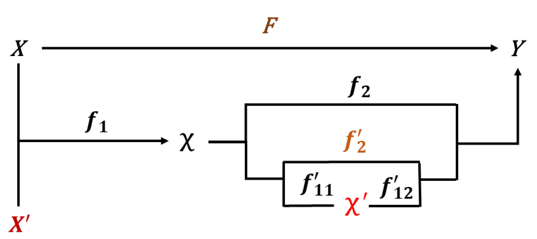
Figure 2.
This is a scatter plot between ERA5_Vmax and IBTrACS_Vmax in the entire dataset.
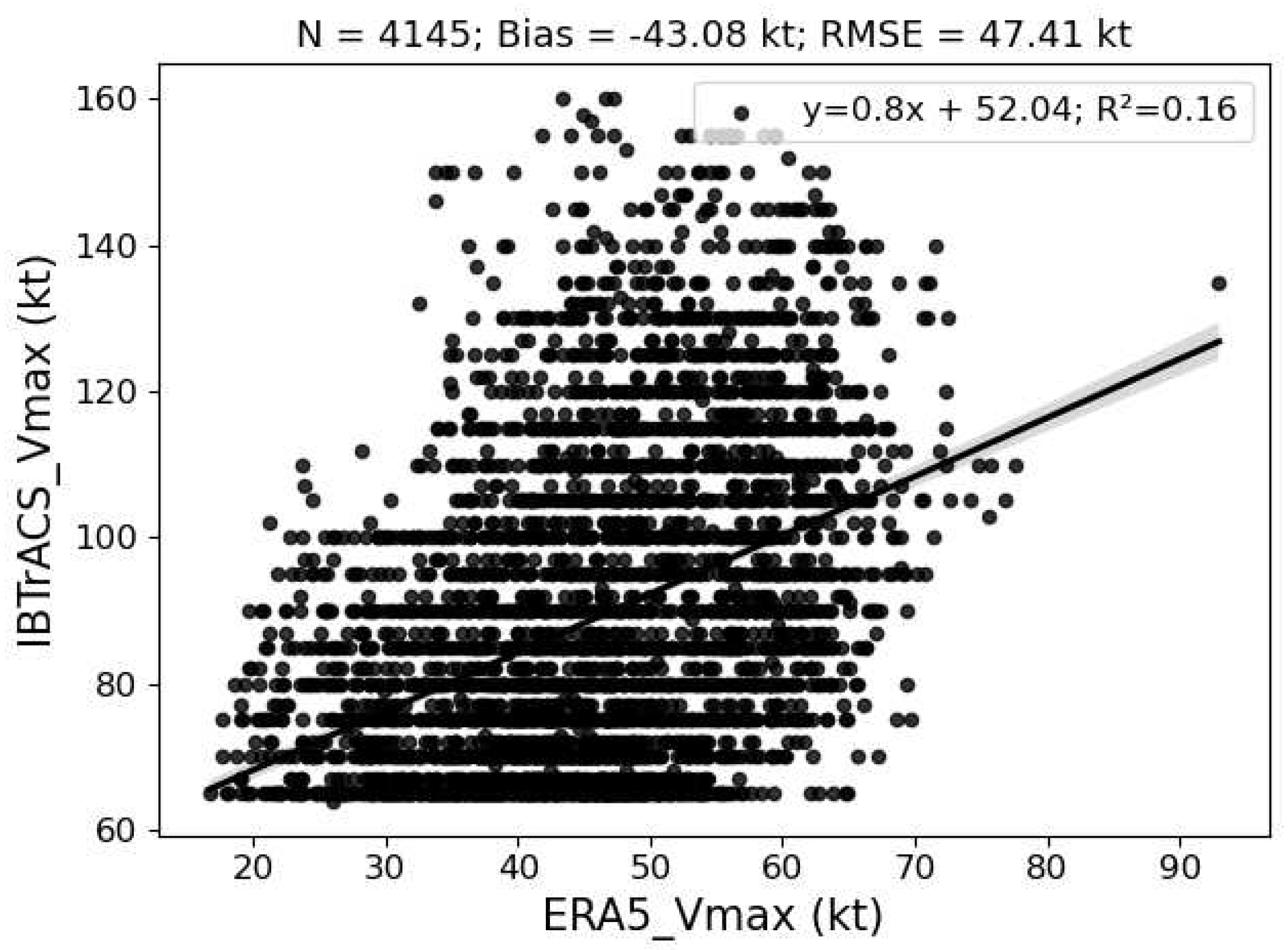
Figure 3.
This is the cumulative curve of RMSE in the entire dataset.
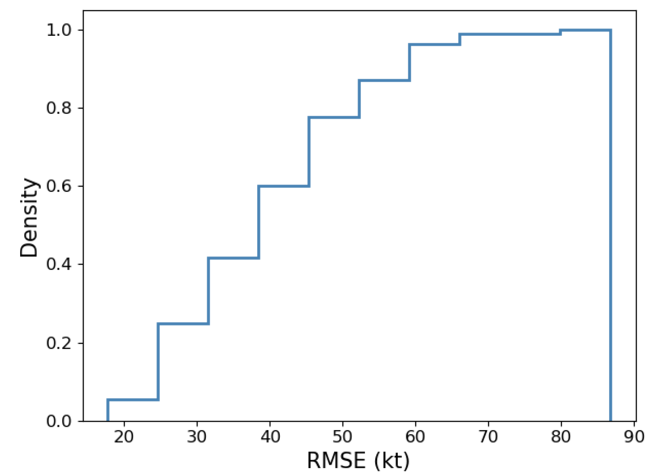
Figure 4.
This is a figure to show the error distribution with different factors. (a) The Bias and RMSE in different years. (b) The Bias and RMSE in different categories.
Figure 4.
This is a figure to show the error distribution with different factors. (a) The Bias and RMSE in different years. (b) The Bias and RMSE in different categories.
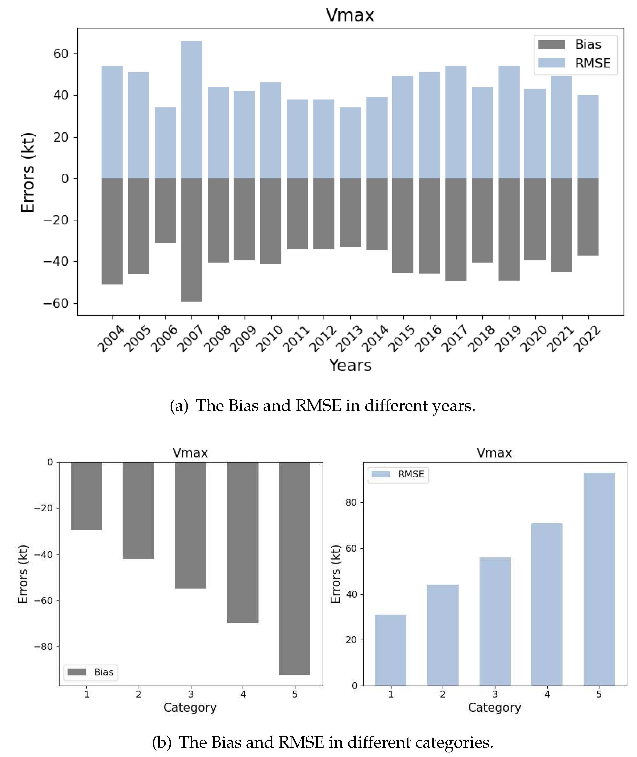
Figure 5.
This is a figure to show the correspondence of Life Maximum Intensity (LMI) of different category storms.
Figure 5.
This is a figure to show the correspondence of Life Maximum Intensity (LMI) of different category storms.
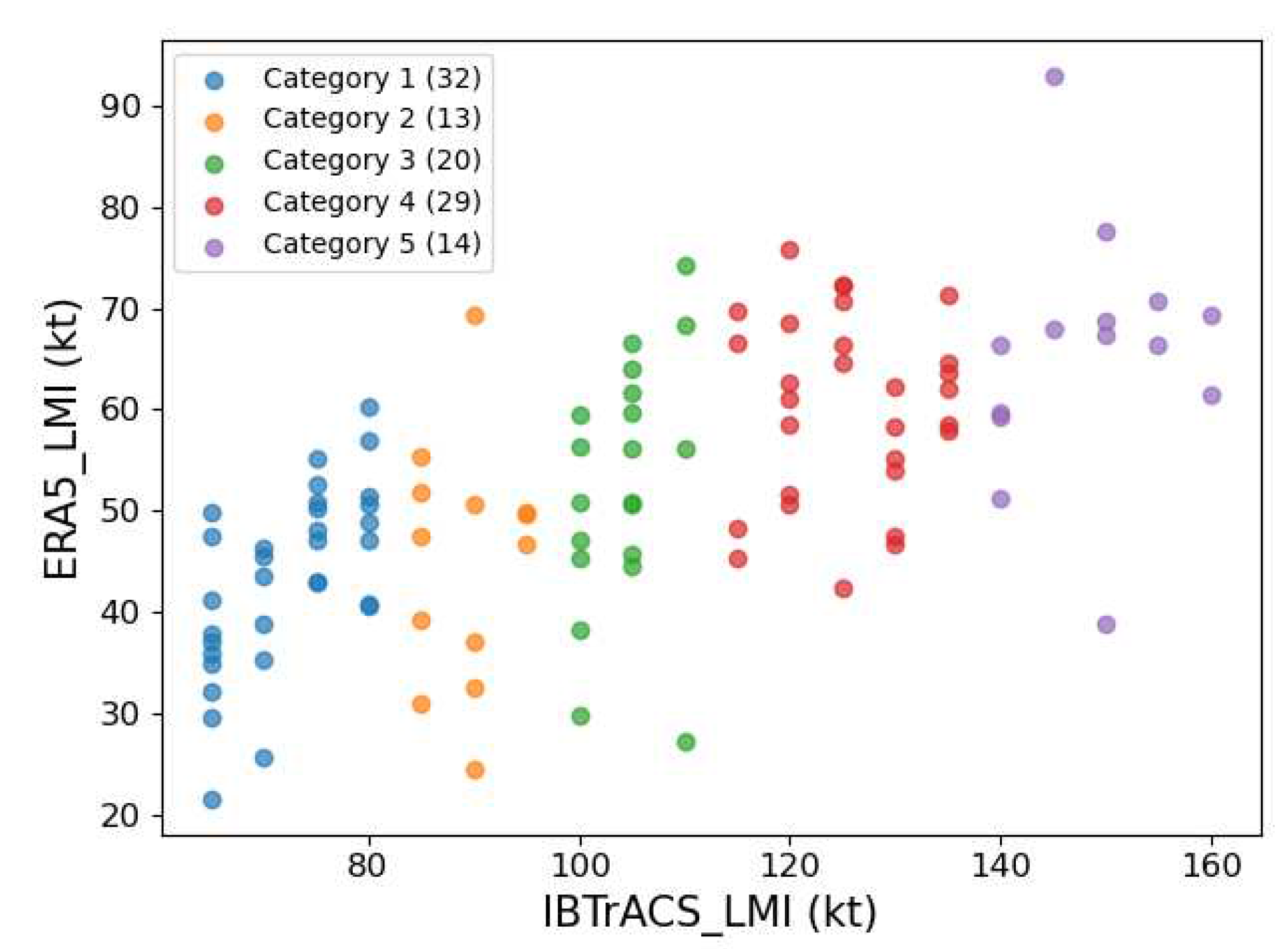
Figure 6.
This is a figure showing the data distribution of the labels in the training dataset (marked as train), validation dataset (val) and testing dataset (test) from three splitting methods. (a) shows the first method, which uses 80% for training, 10% for validation and 10% for testing. And the average value of train and val are around 88 kts with the variance of 21 kts, but a difference value with test about 2 kts. (b) demonstrates the second methods, that is using the 2021-2022 samples for testing, and the rest is split into training and validation dataset. The mean and variance are similar to the first. (c) demonstrates the third method, using the 2004-2018 samples for training, 2019-2020 for validation and 2021-2022 for testing the model. Here, the average value of val and test are close, slightly different with the training dataset.
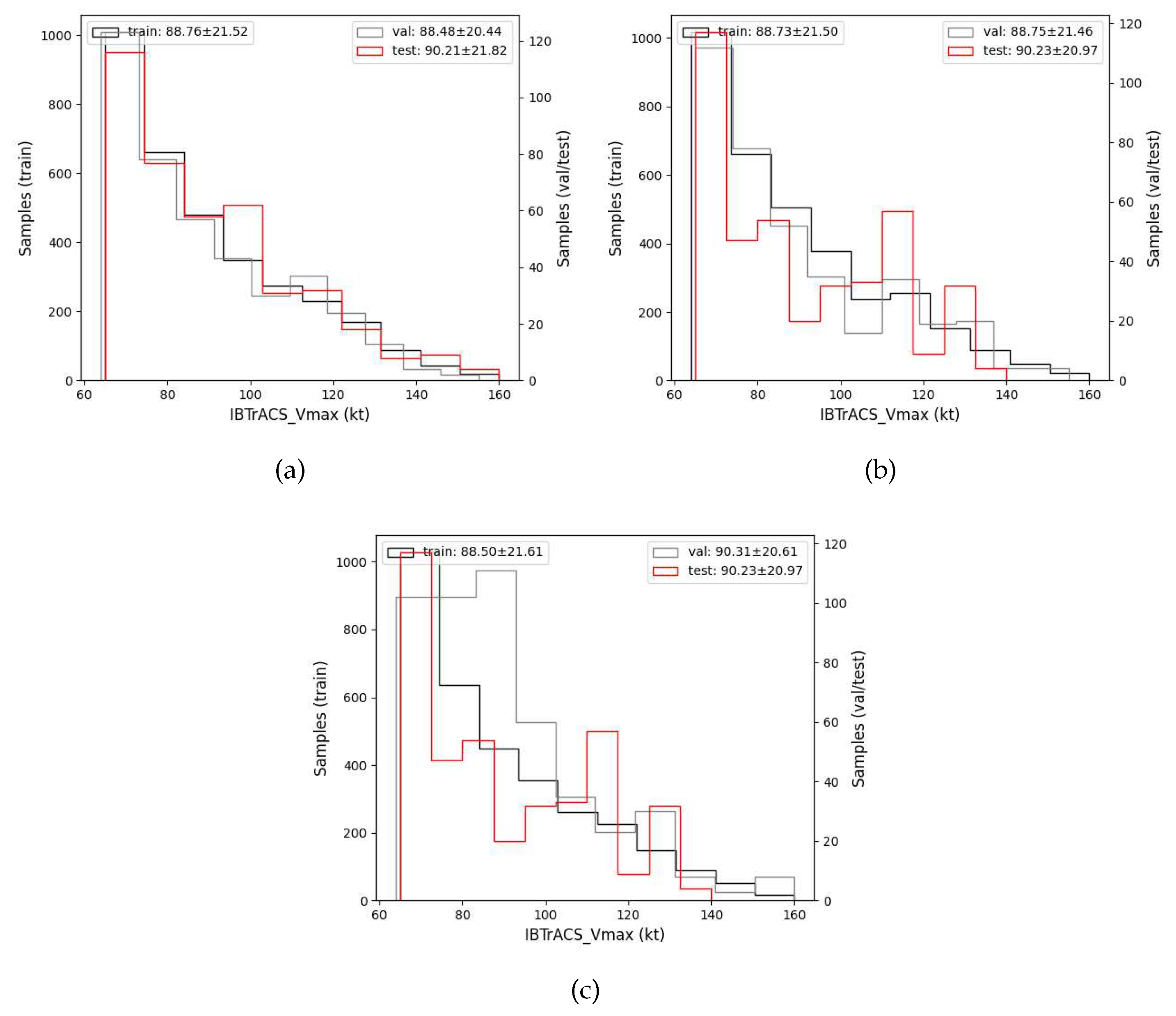
Figure 7.
This is a figure showing the difference between the surface wind pattern and 850 hPa. The colour bars are set to the same range and the unit is kts.
Figure 7.
This is a figure showing the difference between the surface wind pattern and 850 hPa. The colour bars are set to the same range and the unit is kts.
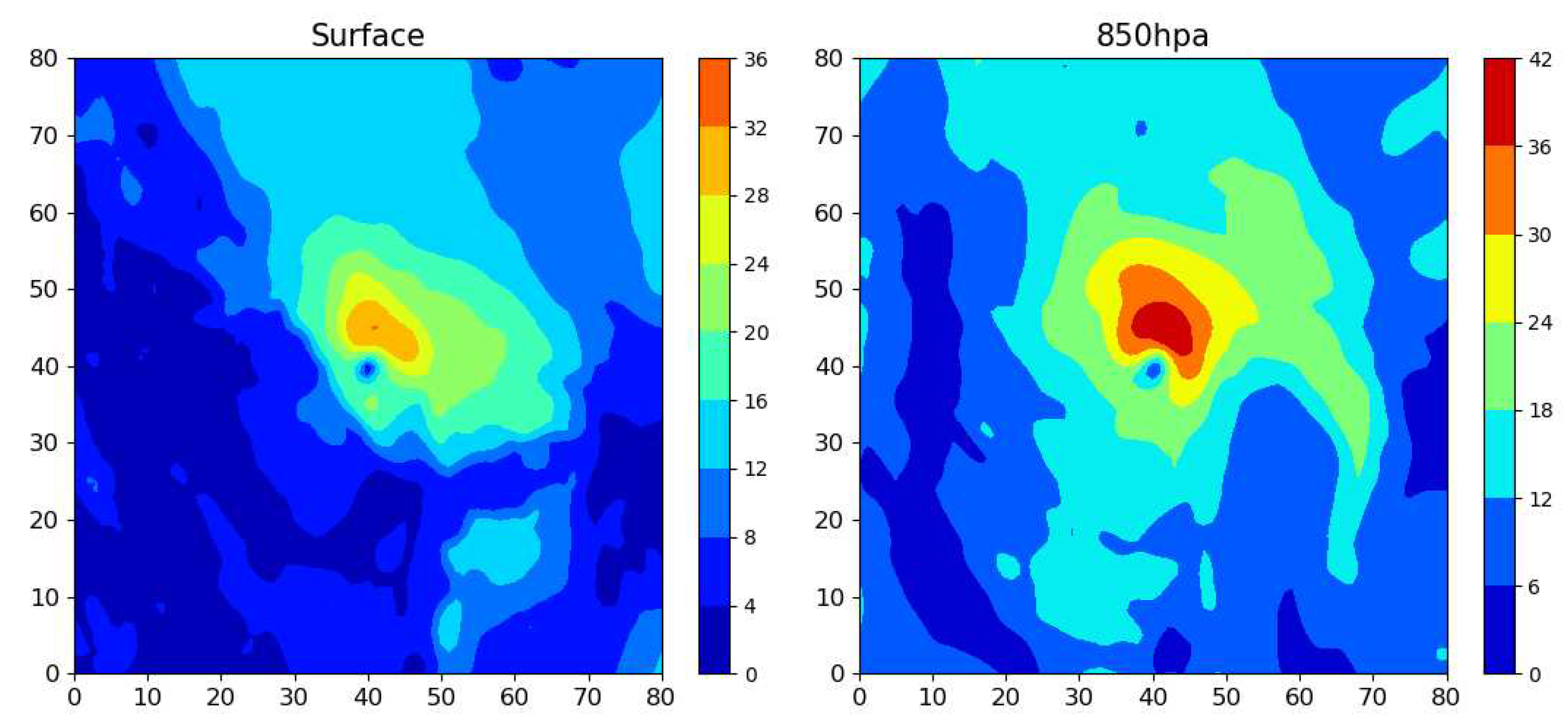
Figure 8.
This is a figure to show the correlation between the prediction of ResNet-18 and the labels of IBTrACS in testing dataset using three data splitting methods.
Figure 8.
This is a figure to show the correlation between the prediction of ResNet-18 and the labels of IBTrACS in testing dataset using three data splitting methods.
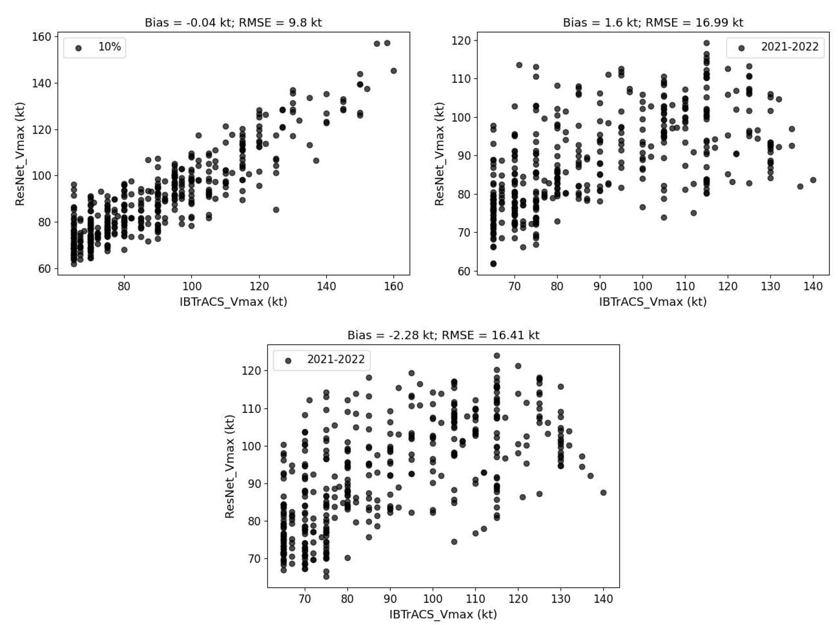
Figure 9.
This is a figure to show three types of data processing methods.And the red arrow in the figure is the storm direction.
Figure 9.
This is a figure to show three types of data processing methods.And the red arrow in the figure is the storm direction.
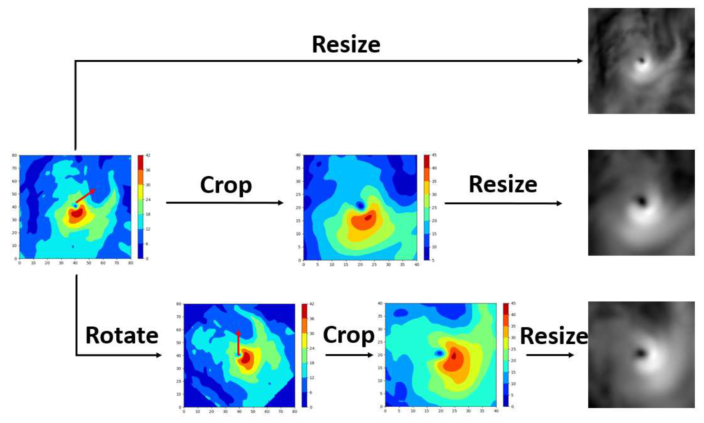
Figure 10.
This is a figure to show the process of retrain the model using the domain adaptation. In the box, fc1 and fc2 are the full connected layers of neural networks.
Figure 10.
This is a figure to show the process of retrain the model using the domain adaptation. In the box, fc1 and fc2 are the full connected layers of neural networks.
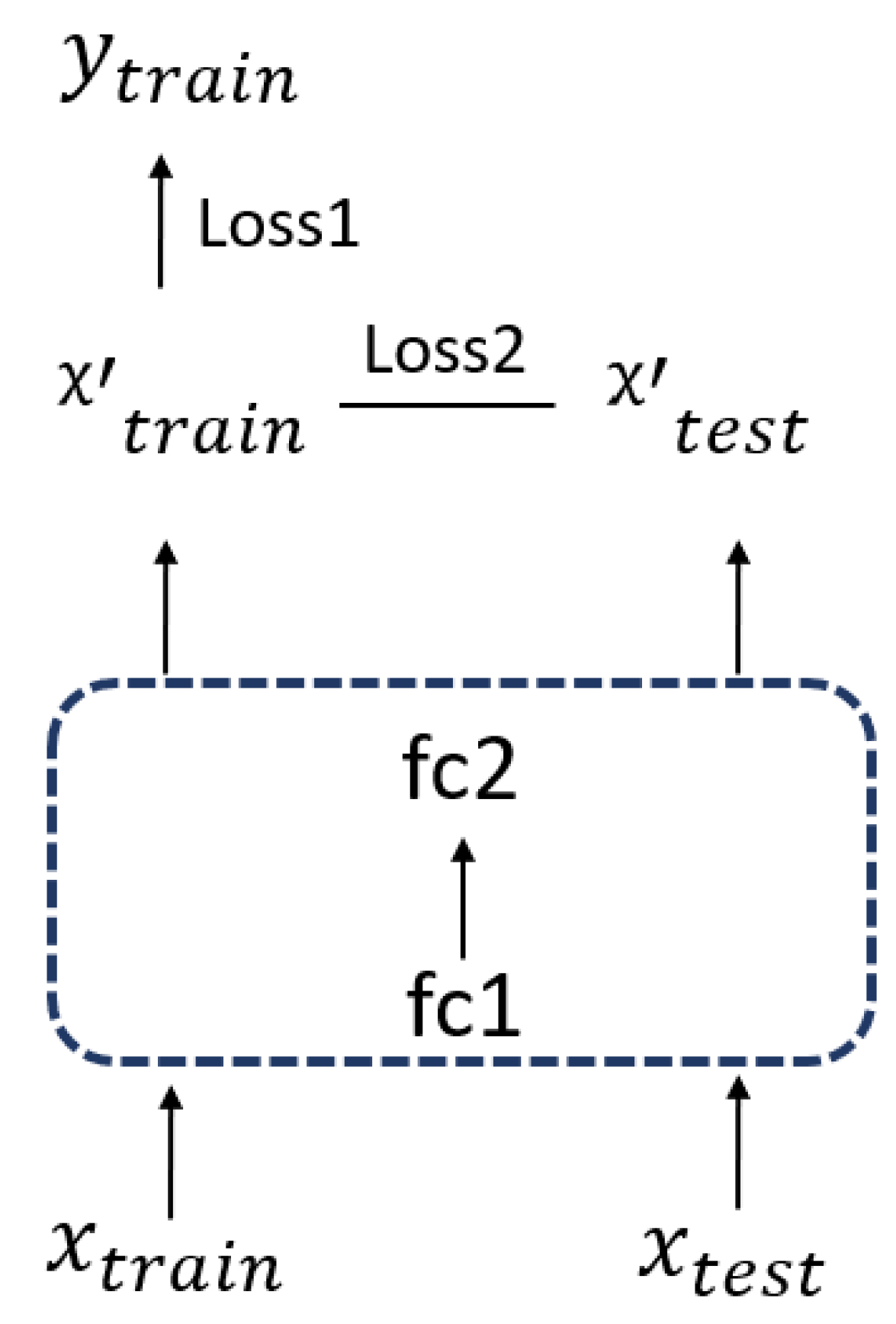
Figure 11.
This is a figure to show the error and prediction distribution of domain adaptation methods with the mmd weight as 100.
Figure 11.
This is a figure to show the error and prediction distribution of domain adaptation methods with the mmd weight as 100.
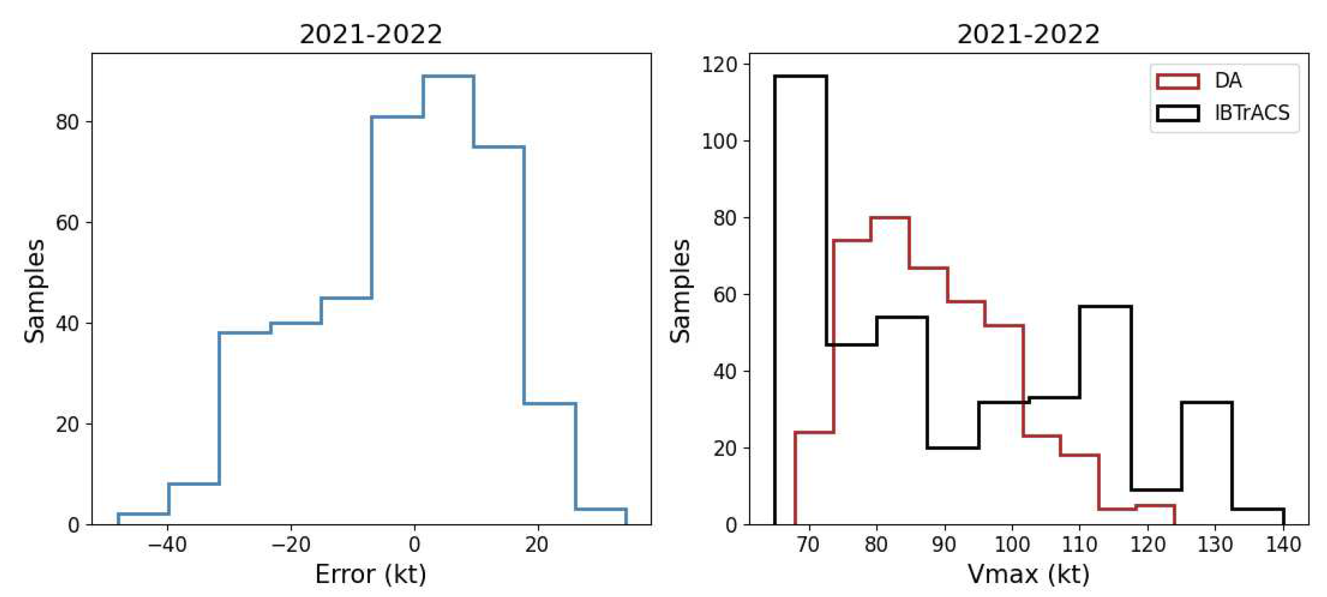

Table 1.
This is the data description of IBTrACS.
| Variable name (units) | Maximum Sustained Wind Speed (kts) Storm Center (degrees lat/lon) Other variables |
| Temporal resolution | Interpolated to 3 hourly (most data reported at 6 hourly) |
| Coverage | 70 N to 70 S and 180 W to 180 E 1841 - present (Not all storms captured) |
Table 2.
This is the data description of ERA5 reanalysis.
| Data type | Gridded |
|---|---|
| Horizontal coverage | Global |
| Horizontal resolution | 0.25 × 0.25 |
| Vertical coverage | 1000 hPa to 1 hPa |
| Vertical resolution | 37 pressure levels |
| Temporal coverage | 1940 to present |
| Temporal resolution | Hourly |
Table 3.
This is the samples collected from North Altantic in IBTrACS.
| TC Numbers | Samples | |
|---|---|---|
| Category 1 (64 ≤ W < 83) | 32 | 2061 |
| Category 2 (83 ≤ W < 96) | 13 | 774 |
| Category 3 (96 ≤ W < 113) | 20 | 626 |
| Category 4 (113 ≤ W < 137) | 29 | 562 |
| Category 5 (W ≥ 137) | 14 | 122 |
| Total | 108 | 4145 |
Table 4.
This is a the overlap rate of different category storms in ERA5 and IBTrACS.
| 10% | 20% | 30% | 40% | 50% | |
|---|---|---|---|---|---|
| Category 1 | 0.00 | 0.33 | 0.60 | 0.77 | 0.75 |
| Category 2 | 0.00 | 0.00 | 0.25 | 0.40 | 0.50 |
| Category 3 | 0.50 | 0.50 | 0.33 | 0.50 | 0.70 |
| Category 4 | 0.00 | 0.17 | 0.11 | 0.25 | 0.43 |
| Category 5 | 0.00 | 0.33 | 0.50 | 0.33 | 0.57 |
Table 5.
This is a table to show the errors (Bias and RMSE) of testing dataset in original dataset and the results after linear correction.
Table 5.
This is a table to show the errors (Bias and RMSE) of testing dataset in original dataset and the results after linear correction.
| Data | Method | Testing dataset (10%) | Testing dataset (2021-2022) | ||
|---|---|---|---|---|---|
| Bias (kts) | RMSE (kts) | Bias (kts) | RMSE (kts) | ||
| Surface | Point to Point | -66.65 | 69.82 | -65.16 | 67.98 |
| Linear model | -1.48 | 20.86 | 1.08 | 19.01 | |
| 850 hPa | Point to Point | -52.48 | 56.7 | -49.72 | 53.6 |
| Linear model | -1.51 | 21.04 | 0.53 | 19.74 | |
Table 6.
This is a table to show the errors (Bias and RMSE) of ResNet-18 in testing dataset using three data splitting methods.
Table 6.
This is a table to show the errors (Bias and RMSE) of ResNet-18 in testing dataset using three data splitting methods.
| Data | Testing dataset (10%) | Testing dataset (2021-2022) | ||||
|---|---|---|---|---|---|---|
| validation (10%) | validation (10%) | validation (2019-2020) | ||||
| Bias (kts) | RMSE (kts) | Bias (kts) | RMSE (kts) | Bias (kts) | RMSE (kts) | |
| Surface | 0.70 | 11.03 | -0.64 | 16.06 | -1.99 | 16.67 |
| 850 hPa | -0.04 | 9.8 | 1.60 | 16.99 | -2.28 | 16.41 |
Table 7.
This is a table to show the results of comparative experiments using different data processing methods.
Table 7.
This is a table to show the results of comparative experiments using different data processing methods.
| Data augmentation | Inputs shape | Bias (kts) | RMSE (kts) |
|---|---|---|---|
| Original | (81, 81, 1) | 0.88 | 17.46 |
| Crop + Resize | (224, 224, 1) | -1.54 | 15.21 |
| Rotate + Crop + Resize | (224, 224, 1) | -1.56 | 16.08 |
Table 8.
This is a table to show the results of comparative experiments using different data processing methods.
Table 8.
This is a table to show the results of comparative experiments using different data processing methods.
| Variables | Layers | Inputs shape | ResNet-18 | |
|---|---|---|---|---|
| Bias (kts) | RMSE (kts) | |||
| Wind | 850 hPa, 200 hPa | (224, 224, 2) | -0.66 | 16.19 |
| 850 hPa, 500 hPa | (224, 224, 2) | -1.11 | 16.60 | |
| 850 hPa, 500 hPa, 200 hPa | (224, 224, 3) | -1.36 | 15.47 | |
| Wind, | 850 hPa | (224, 224, 2) | 0.54 | 18.00 |
| 850 hPa, 200 hPa | (224, 224, 4) | -0.52 | 16.45 | |
| 850 hPa, 500 hPa | (224, 224, 4) | 2.32 | 17.03 | |
| 850 hPa, 500 hPa, 200 hPa | (224, 224, 6) | 0.82 | 14.90 | |
Table 9.
This is a table to show the results of comparative experiments using different fold to enlarge the training dataset.
Table 9.
This is a table to show the results of comparative experiments using different fold to enlarge the training dataset.
| Fold | Sample size (Training dataset) | Bias (kts) | RMSE (kts) |
|---|---|---|---|
| 0 | 3258 | 0.82 | 14.90 |
| 1 | 6516 | -2.43 | 15.47 |
| 2 | 9774 | -1.07 | 14.76 |
| 3 | 13032 | -0.77 | 15.16 |
| 4 | 16290 | -0.26 | 15.14 |
Table 10.
This is a table to describe three splitting methods to update the datset using the features from trained model in previous dataset.
Table 10.
This is a table to describe three splitting methods to update the datset using the features from trained model in previous dataset.
| Training dataset () | Validation dataset () | Testing dataset () | |
|---|---|---|---|
| D1 | (, ) | (, ) | (, ) |
| D2 | 90% of (, ) | 10% of (, ) | (, ) |
| D3 | 90% of (, ) + (, ) | 10% of (, ) + (, ) | (, ) |
Table 11.
This is a table to show the results of comparative experiments using different methods and different dataset for updating feature and feature-output mapping.
Table 11.
This is a table to show the results of comparative experiments using different methods and different dataset for updating feature and feature-output mapping.
 |
Disclaimer/Publisher’s Note: The statements, opinions and data contained in all publications are solely those of the individual author(s) and contributor(s) and not of MDPI and/or the editor(s). MDPI and/or the editor(s) disclaim responsibility for any injury to people or property resulting from any ideas, methods, instructions or products referred to in the content. |
© 2023 by the authors. Licensee MDPI, Basel, Switzerland. This article is an open access article distributed under the terms and conditions of the Creative Commons Attribution (CC BY) license (http://creativecommons.org/licenses/by/4.0/).
Copyright: This open access article is published under a Creative Commons CC BY 4.0 license, which permit the free download, distribution, and reuse, provided that the author and preprint are cited in any reuse.


