
Submitted:
12 October 2023
Posted:
16 October 2023
Read the latest preprint version here
Abstract
Detecting abrupt transitions in ecosystems, known as regime shifts, holds immense implications for conservation and management endeavors. This research aims to investigate the feasibility of developing an early warning system capable of identifying an upcoming critical transition within Mangrove Forest ecosystems. Employing a fusion of remote sensing analysis, time series analysis, and the critical slowing down theory, Mangrove Forests' state change was explored across two distinct study sites. One site has been adversely affected by disturbances stemming from land use and land cover changes, while the other serves as an unaffected reference ecosystem. The study uses data from the Moderate Resolution Imaging Spectroradiometer (MODIS) satellite, quantifying three remotely sensed indices: the Normalized Difference Vegetation Index (NDVI), the Modified Normalized Difference Water Index (MNDWI), and the Modified Vegetation Water Ratio (MVWR). Furthermore, temporal alterations in land-use and land cover are scrutinized using Landsat data from 1996, 2002, 2008, and 2014. To identify early warning signals of critical transitions, indicators such as autocorrelation, skewness, and standard deviation are applied. The results show the robust capabilities of remote sensing in generating early warning signals of critical transition in Mangrove Forests. NDVI outperformed MVWR and MNDWI as ecosystem state indicators. This study not only highlights the potential of remote in identifying the approaching regime shifts in Mangrove Forest ecosystems but also adds knowledge on ecosystem dynamics. This is the first report of the successful application of remote sensing in generating early warning signals for imminent critical transitions within Mangrove forests in the Middle East.
Keywords:
land-use and land cover-change
; monitoring ecosystem dynamics
; remote sensing
; Mangrove forests
1. Introduction
Mangrove forests play a crucial role in providing valuable ecosystem services, contributing to a staggering annual value of at least US $1.6 billion (Polidoro, Carpenter et al. 2010). These services encompass a wide range of benefits that support coastal livelihoods on a global scale (Dahdouh-Guebas, Jayatissa et al. 2005, Duke, Meynecke et al. 2007, Ellison 2008, Abrantes, Johnston et al. 2015). However, Mangrove forests are disappearing worldwide by 1 to 2% per year (Duke, Meynecke et al. 2007). Clearing for coastal development, expansion of aquaculture, logging for timber, and fuel production are among the primary drivers behind this concerning trend (Daru, Yessoufou et al. 2013, Kirui, Kairo et al. 2013, Yessoufou and Stoffberg 2016). It has been shown that over 40% of the assessed vertebrate species endemic to Mangrove Forests are currently facing global threats to their survival (Luther and Greenberg 2009). As a result, urgent attention is needed to monitor the state of Mangrove forests and get a better understanding of Mangrove Forest dynamics in response to disturbances.
The response of an ecosystem, such as the Mangrove ecosystem, to disturbance is not always a gradual process; it can lead to sudden and irreversible changes (Scheffer 1990, Scheffer 2001, Scheffer, Carpenter et al. 2001). In fact, even gradual changes in the environment may not result in a corresponding gradual response from the ecosystem. Instead, they can trigger sudden, unpredictable, and irreversible shifts known as regime shifts (Capon, Lynch et al. 2015). Apart from the growing evidence of critical changes occurrences in different ecosystems (Barbier, Koch et al. 2008, Guttal and Jayaprakash 2008, Lenton 2011, Verbesselt, Umlauf et al. 2016, Alibakhshi, Groen et al. 2017), the need to enhance the understanding of generating early warning signals of critical transition in ecosystems is highlighted.
Abrupt changes in the state of an ecosystem can occur when ecosystems are unable to cope with the effects of disturbances, leading to slower resilience and a reduced ability to recover (Carpenter and Brock 2006, Carpenter, Brock et al. 2008, Scheffer, Bascompte et al. 2009, Carpenter and Brock 2011, Carpenter, Cole et al. 2011). Disturbances can push the state of an ecosystem to a state that is near a critical threshold. Once a critical threshold is reached, even a small disturbance can trigger a significant transition to a new state, where it is challenging and sometimes impossible to return to the previous state (Scheffer, Carpenter et al. 2001, Carpenter and Brock 2006, Carpenter, Brock et al. 2008, Scheffer, Bascompte et al. 2009, Carpenter and Brock 2011, Carpenter, Cole et al. 2011). This knowledge is crucial for assessing the current state of an ecosystem and determining whether it is approaching a critical transition. Understanding the current state of an ecosystem is particularly crucial in Mangrove Forests, as it can inform conservation efforts and has abundant resources and socio-economic impacts for locals (Martínez, Intralawan et al. 2007). Detecting the state of an ecosystem can prevent irreversible changes and facilitate early interventions (Lenton, Held et al. 2008, Hirota, Holmgren et al. 2011, Alibakhshi 2023).
Various methods have been developed to quantify the state of an ecosystem (Carpenter and Brock 2006, Dakos, Carpenter et al. 2012, Kéfi, Guttal et al. 2014). For example, an increasing trend in autocorrelation and standard deviation of the state variables over time (Dakos, Van Nes et al. 2012) can serve as reliable early warning signals, indicating an approaching critical transition in the ecosystem (Dakos, Carpenter et al. 2012, Dakos, Van Nes et al. 2012, Lenton, Livina et al. 2012, Dakos, Carpenter et al. 2015). Furthermore, disruptions or disturbances within the ecosystem can lead to alterations in the asymmetrical distribution of the state variable time series, resulting in an increased skewness, which can be served as early warning signals of critical transition (Guttal and Jayaprakash 2008, Dakos, Carpenter et al. 2012).
Despite the availability of various methods for assessing early warning signals (Eslami-Andergoli, Dale et al. 2015), the anticipation of critical transitions in ecosystems poses significant challenges. Hence, the application of the methods to assess the state of ecosystems and identify early warning signals of critical transition in the state of ecosystems is still limited. The complexity and diversity of ecological systems, coupled with the need for high-frequency observations and comprehensive time series data on relevant environmental variables, present significant obstacles (Dakos, Carpenter et al. 2015). To address this problem, this study is using the high spatio-temporal resolution of satellite images. Satellite images offer high-resolution, comprehensive coverage, and multispectral capabilities, making them a powerful tool for the aim of this study.
To effectively detect the approach of an ecosystem towards a critical threshold, it is crucial to select the right state variables, which is variable that can accurately present the state of an ecosystem and measure the proximity of the ecosystem to critical conditions (Alibakhshi, Groen et al. 2017). For example, a research study has demonstrated that the utilization of remotely sensed indicators capable of simultaneously capturing variations in both water and vegetation can provide a more comprehensive understanding of the state of an ecosystem compared to relying solely on vegetation-based or water-based indices (Alibakhshi, Groen et al. 2017).
This study aims to investigate the potential of time series analysis of remote sensing data in detecting regime shifts in Mangrove Forest ecosystems and establishing an early warning system. As two main components of Mangrove Forests are vegetation and water, a vegetation-based indicator, namely the Normalized Difference Vegetation Index (NDVI), a water-based indicator, namely the Modified Normalized Difference Water Index (MNDW), and a vegetation-water-based indicator, namely Modified Vegetation Water Ratio (MVWR) has been employed as remotely sensed state variables. Additionally, changes in land-use and land cover-change are quantified using Landsat data from 1996, 2002, 2008, and 2014 to assess the reasons behind the reduced resilience and possible early warning signals of upcoming critical transition in study sites. Mangrove Forest ecosystems in Qeshm Island and Gabrik are chosen as case studies, where Qeshm Island is selected as a representative of an unhealthy ecosystem, while Gabrik serves as the reference site for comparison. The application of critical slowing down in monitoring Mangrove Forests has been rarely tested (Wang, Zhang et al. 2023). This is the first study that explores the potential of remote sensing to explore early warning signals of impending critical transition in Mangrove forests in Iran.
2. Material and Methods
2.1. Study Area
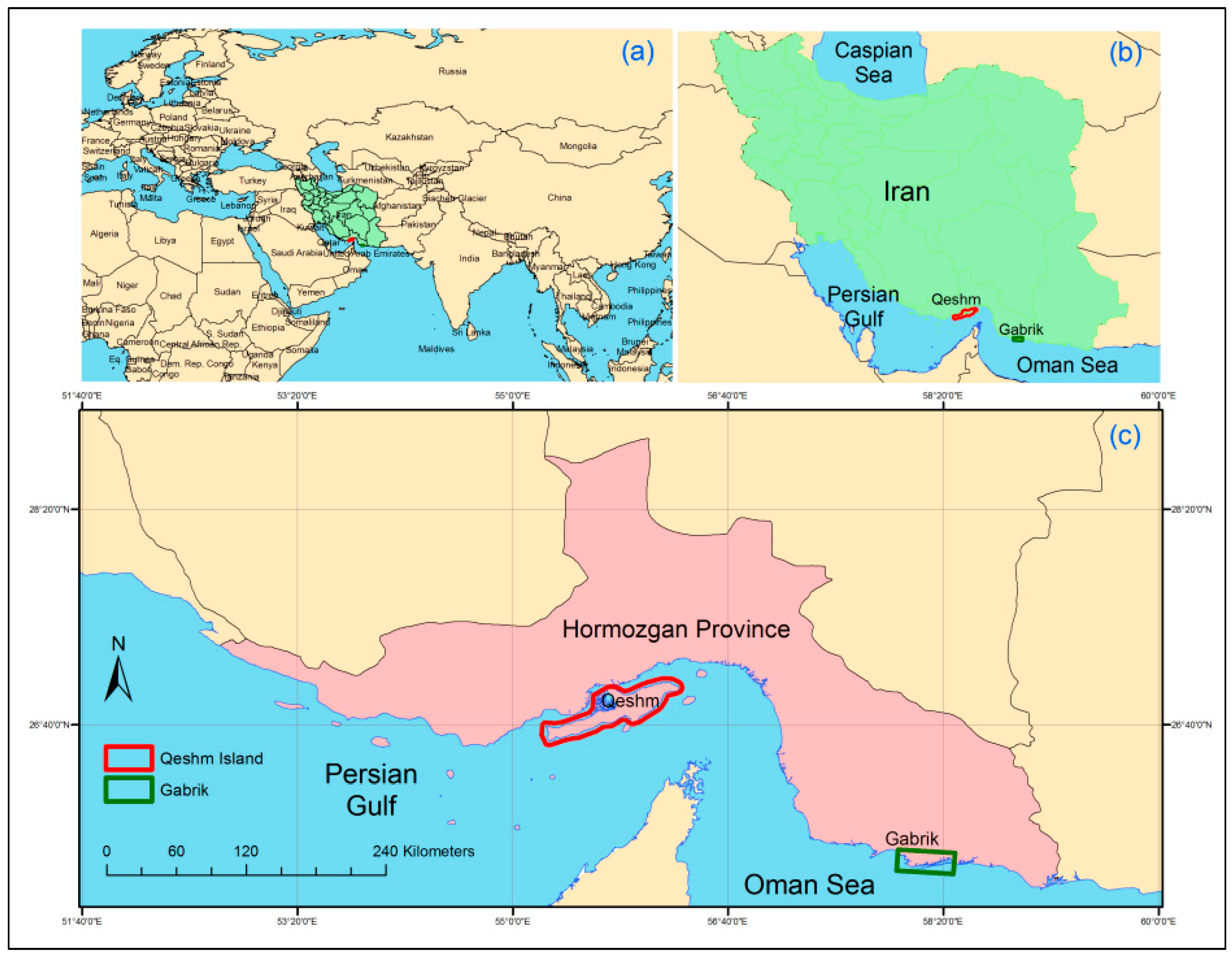
This study focuses on Qeshm Island (Mazraeh and Pazhouhanfar 2018, Kourosh Niya, Huang et al. 2019), located in the southern region of Iran, between the Persian Gulf and the Oman Sea. Qeshm Island, with a total area of 1667 km2, has undergone substantial and, at times, drastic changes in its land-use and land cover-change time (Kourosh Niya, Huang et al. 2019). Gabrik, with a total area of 2496 km2, has been selected as a reference case study, representing a healthy ecosystem. Gabrik shares identical climatic conditions with Qeshm Island and is also characterized by the presence of Mangrove Forest ecosystems (Zahed, Rouhani et al. 2010, Naderloo, Türkay et al. 2013).
The geographical coordinates of Qeshm Island range from 55° 15’ 38” to 56° 16’ 52” E and 26° 32’ 20” to 27° 00’ 00” N, and Gabrik is located southeast of Qeshm Island with geographical coordinates ranging from 55° 15’ 38” to 56° 16’ 52” E and 26° 32’ 20” to 27° 00’ 00” N (Figure 1). Based on ERA5 data (Muñoz Sabater 2019), the mean temperature in Qeshm Island is 301 Kelvin (28 degrees Celsius), and the mean precipitation is 36 mm from February 18, 2000 to July 31, 2021. In Gabrik, the mean temperature is 301 Kelvin (28 degrees Celsius), with an average precipitation of 28 mm from February 18, 2000 to July 31, 2021. These show the similarity of climatic conditions and local weather patterns of Qeshm Island and Gabrik study sites (Figure 1). According to the population dataset provided by WorldPop (Sorichetta, Hornby et al. 2015), the estimated population residing in the region of Gabrik is reported to be remarkably low, with a mere 74 individuals. On the other hand, a significantly higher population count of 957 individuals are living in Qeshm Island.
Figure 1.
Monthly temperature in Kelvin (°K) and precipitation millimetres (mm) for Qeshm Island and Gabrik from February 18, 2000, to July 31, 2021.
Figure 1.
Monthly temperature in Kelvin (°K) and precipitation millimetres (mm) for Qeshm Island and Gabrik from February 18, 2000, to July 31, 2021.
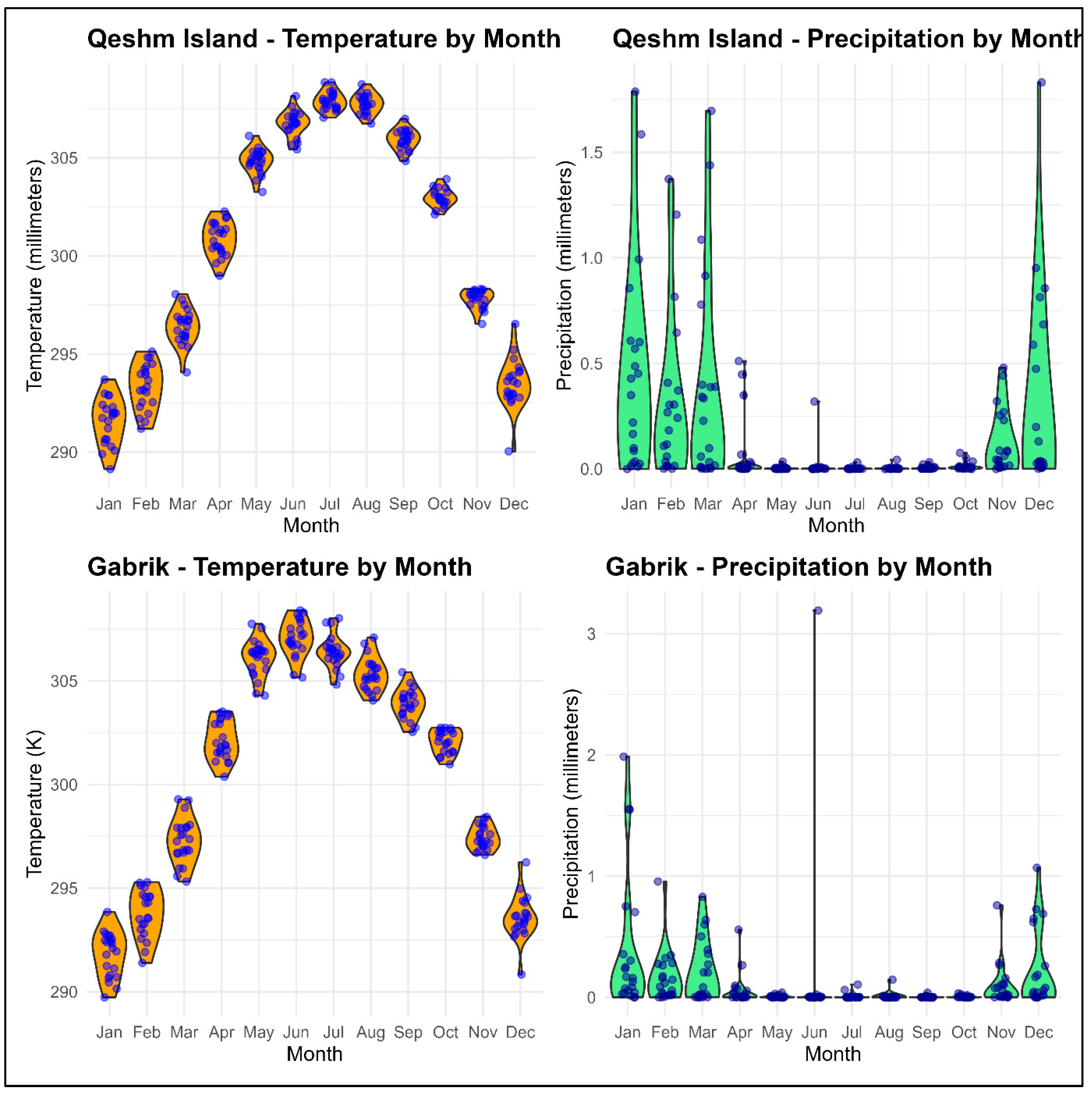
Figure 2.
Location of the study sites Qeshm Island and Gabrik (a:c).
2.2. Materials and data collection
2.2.1. State variables
The Normalized Difference Vegetation Index has been obtained from the latest version of the Moderate Resolution Imaging Spectroradiometer (MODIS) product, specifically MOD09A1 (version 006). The 006 version of MOD09A1 has undergone algorithm enhancements aimed at improving its accuracy (Didan, 2015). The data utilized in this study was acquired from the Google Earth Engine platform (Gorelick et al., 2017), which offers a comprehensive repository of geospatial data. The dataset utilized herein possesses a spatial resolution of 500 meters with a temporal resolution of 16 days, enabling comprehensive analysis from February 18, 2000, to July 31, 2021. The MOD09A1 product is derived from atmospherically corrected bi-directional surface reflectance. The Red and Near-Infrared (NIR) bands, specifically within the wavelengths of 0.620 μm to 0.670 μm and 0.841 μm to 0.876 μm, respectively has been used to calculate NDVI (Eq. 1). The NDVI values range from -1 to +1, where a value of -1 indicates bare land, while a value of +1 indicates dense forest.
Furthermore, the Modified Normalized Difference Water Index (MNDWI) is a useful indicator for identifying and quantifying water bodies within an ecosystem (Xu 2006). MNDWI is calculated using MOD09A1 (version 006), which is described earlier. Among the numerous remotely sensed water indices available (Mozumder, Tripathi et al. 2014, Rokni, Ahmad et al. 2014, Li, Chen et al. 2015), MNDWI has been recognized as the most accurate indicator for extracting water area variations (Ji, Zhang et al. 2009, Chen, Huang et al. 2013). MNDWI, similar to NDVI, is a dimensionless index that ranges from -1 to 1. When MNDWI values are below 0, it indicates low water content, which includes soil and vegetation. On the other hand, MNDWI values above 0 indicate high water content and varying water levels. The Green and shortwave infrared (SWIR) bands, specifically within the wavelengths of 1.23 μm to 1.25 μm and 0.55 μm to 0.57 μm, respectively has been used to calculate MNDWI) (Eq. 2).
Additionally, the Modified Vegetation Water Ratio (MVWR) was used to measure early warning signs in aquatic ecosystems (Alibakhshi, Groen et al. 2017) (Eq. 3). The MVWR is sensitive to changes in vegetation water content, which are the main component of Mangrove Forests. It effectively captures variations in water availability and reflects hydrological dynamics, such as seasonal fluctuations and long-term shifts. Moreover, the MVWR proves valuable in assessing vegetation health and stress levels (Tehrani and Janalipour 2021).
2.2.2. Map of mangrove Forest ecosystems and land-use and land cover-change
The land-use and land cover-changes map was calculated with a spatial resolution of 30 meters (Kourosh Niya, Huang et al. 2019), by using Landsat satellite imagery for the years 1996, 2002, 2008, and 2014. The maps provide a classification map of study sites, including six distinct land use classes: agriculture, bare-land, built-up, dense-vegetation, mangrove (Mangrove Forest ecosystem), and waterbody.
In addition, the Global Mangrove Forest Distribution dataset was employed for the year 2000 which provides a map of the world’s Mangrove Forest ecosystems as of the year 2000 with a spatial resolution of approximately 30 meters (Giri, Ochieng et al. 2011, Giri, Ochieng et al. 2013). The data compilation involved analyzing over 1,000 Landsat Thematic Mapper (TM) scenes using a hybrid approach of classification techniques.
2.3. Methods for exploring early warning signals of critical transition
In this study, we only used a large variety of freely available remotely sensed data. All statistical analyses and visualizations were performed in R statistical software (Pinheiro, Bates et al. 2000) QGIS (Qgis 2016), and Google Earth Engine (Gorelick, Hancher et al. 2017).
First Mangrove Forest ecosystems in each study site were delineated using the Global Mangrove Forest Distribution maps (Section 2.2.2). Second, 100 points in each study site were randomly selected. From each point, the time series of the state variables (Section 2.2.1) was extracted using a mean function for the period from February 18, 2000, to July 31, 2021. Finally, autocorrelation, skewness, and standard deviation were applied to detect early warning signals of critical transition (Dakos, Carpenter et al. 2012). More specifically, autocorrelation refers to the degree of correlation between the values of the same variables in different observations in the data. The concept of autocorrelation is usually used in time series data to calculate the correlation of value to itself in different observations over a consecutive time. For autocorrelation calculation, the first step is to define a lag operator, which is represented by (t) and is a time display. The autocorrelation function (ACF) can be calculated using equation (4):
Standard deviation (SD) measures the degree of variability or distribution for a set of data relative to the mean of the same data. SD is obtained from the variance as shown in equation (5):
Skewness is the third statistical index used in this study, which is calculated using equation (6):
Prior to applying metric-based models, the data needs to undergo detrending and smoothing procedures to mitigate the impact of nonstationary conditions on the leading indicators (Dakos, Carpenter et al. 2012). Several detrending approaches are commonly employed, such as Gaussian, Linear, Loess filters, and first-differencing (Lenton, Livina et al. 2012). These methods detrend the data within a rolling window. In this study, a sensitivity analysis was conducted using Kendall’s τ, a nonparametric statistic measuring the association between indicators and time, to identify the optimal size of the rolling window and bandwidth for the Gaussian filter (Bevan and Kendall 1971). Kendall’s τ ranges from -1 to +1, where higher values indicate stronger trends, aiming to identify the detrending settings that best capture trends in the leading indicators. To achieve this, the leading indicators for various rolling window sizes (ranging from 25% to 75% of the time series length) and bandwidths (ranging from 25% to 75% of the time series length for the Gaussian filter) with increments of 10%, using Gaussian, Loess, Linear filters, and first-differencing approaches was calculated.
To ensure that the observed trends in the leading indicators were not due to random chance, 1000 surrogate datasets were generated. These datasets were created by fitting the best linear autoregressive moving average model (ARMA) based on AIC to the residuals obtained after detrending the data. Each surrogate dataset had the same length as the residual time series. Following previous research, the trend estimations from the original data with those from the surrogate data, had similar correlation structures and probability distributions. Kendall’s τ was employed to estimate trends in autocorrelation, skewness, and standard deviation was compared. The probability of finding a trend by chance was measured by comparing Kendall’s τ of the original data with the number of cases in which the statistic was equal to or smaller than the estimates of the simulated records, denoted as P(τ∗≤τ) (Dakos, Carpenter et al. 2012). Additionally, when a clear breakpoint was present in the time series, Kendall’s τ for the period before the breakpoint was reported to ensure robust trend estimations.
3. Results
The Results include an analysis of land-use and land cover-change in Qeshm Island and Gabrik, highlighting changes in agriculture, bare land, built-up areas, mangroves, vegetation, and water bodies (Section 3.1). Time series of state variables, including NDVI, MNDWI, and MVWR are represented, which show temporal dynamics and seasonal variations of Mangrove Forests in study sites (Section 3.2). Finally, the early warning signals observed time series of NDVI, MNDWI, and MVWR have been presented (Section 3.3).
3.1. land-use and land cover-change
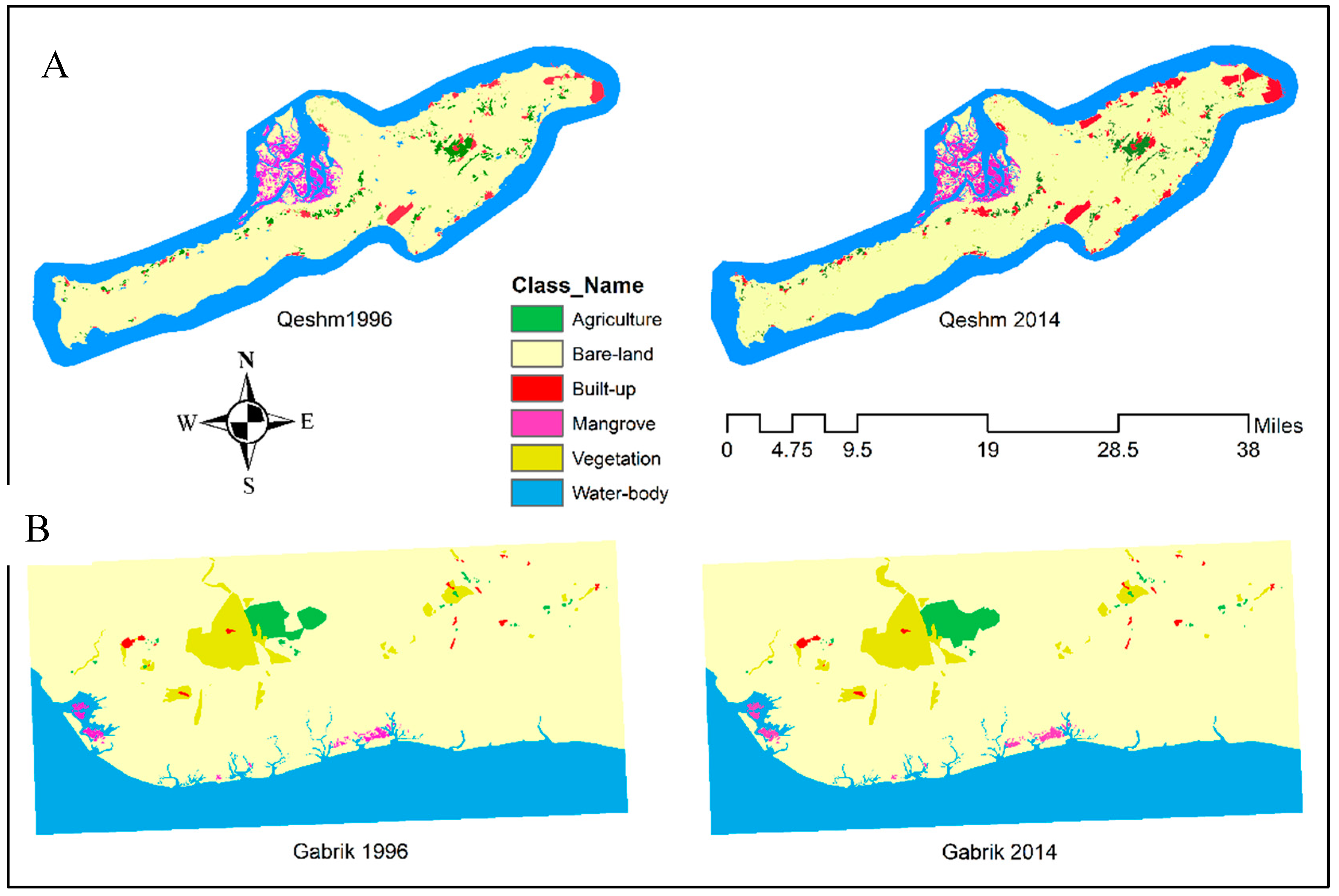
Qeshm Island experienced various changes in land-use and land cover-change during the study period (Table 1). The area dedicated to agriculture witnessed a marginal increase of 338 units (0.65% change). However, there was a significant decrease in bare land, with a change of -57,360 units (-3.65% change). On the other hand, built-up areas expanded dramatically, showing an increase of 35,759 units (64.40% change). Mangroves and vegetation also exhibited positive growth, with changes of 6,049 units (9.07% change) and 6,880 units (70.30% change), respectively. Water bodies slightly expanded, with a change of 8,336 units (0.82% change).
In Gabrik agriculture experienced substantial growth (Table 1), with a change of 4,708 units (15.22% change). Bare land decreased, albeit to a lesser extent, with a change of -8,629 units (-0.52% change). The built-up areas expanded modestly, with a change of 215 units (4.04% change). Mangroves and vegetation also showed positive growth, with changes of 790 units (9.47% change) and 2,628 units (3.22% change), respectively. Water bodies remained relatively stable, with a minimal change of 288 units (0.04% change).
Figure 3.
Land-use maps of Qeshm Island (A) and Gabrik (B) were extracted from Landsat images from 1996 to 2014.
Figure 3.
Land-use maps of Qeshm Island (A) and Gabrik (B) were extracted from Landsat images from 1996 to 2014.
3.2. Time series of state variables
The extracted data for the NDVI, MNDVI, and MVWR indices represent temporal dynamics and seasonal variations in study sites (Figure 5). The data presented in the table consists of four variables: time, NDVI, MNDWI, and MVWR. The time column represents the date of the measurements. The NDVI values range from 0.01 to 0.36, indicating the density of green vegetation cover in the study area. The MNDWI values range from -0.01 to 0.36, representing the presence of water bodies. The MVWR values range from -0.242 to 0.263, indicating the vegetation’s water content. In Gabrik, the NDVI values range from -0.078 to 0.35, indicating the density of green vegetation cover in the study area. The MNDWI values range from -0.10 to 0.27, representing the presence of water bodies. The MVWR values range from -0.25 to 0.27, indicating the vegetation’s water content.
Qeshm Island has a slightly higher average NDVI value of 0.20, indicating a relatively denser green vegetation cover compared to Gabrik, which has an average NDVI of 0.17. This suggests that Qeshm Island may have a higher overall vegetation density. In terms of water presence, Gabrik exhibits a lower average MNDWI value of 0.04, suggesting a relatively lower presence of water bodies compared to Qeshm Island, which has an average MNDWI of 0.10. This indicates that Qeshm Island may have more abundant water bodies within its study area. Regarding vegetation water content, Gabrik and Qeshm Island have similar average MVWR values of 0.10 and 0.09, respectively.
3.3. Early warning signals of a critical transition
Comparing the values obtained for autocorrelation, Qeshm exhibited significantly higher values (0.411, 0.817, and 0.181) compared to Gabrik (0.037, -0.046, and 0.004), indicating a stronger temporal dependency within the ecosystem. Conversely, Gabrik displayed relatively lower autocorrelation values. Furthermore, the analysis of standard deviation demonstrated notably higher values for Qeshm (0.535, 0.827, and -0.207) compared to Gabrik (-0.689, 0.652, and -0.483). Regarding skewness, Qeshm exhibited positive values (0.631, 0.401), while Gabrik displayed negative values (-0.199, -0.191) for NDVI and MNDWI indices. These contrasting skewness values indicate asymmetry in the distribution of the variables.
4. Discussion
This study illuminates the provision of early warning signals for abrupt changes in the Mangrove Forest ecosystem, offering valuable information about the impact of land-use and land cover-change on ecosystem dynamics. Mangrove Forest ecosystems are crucial for biodiversity conservation, harboring a diverse range of plant and animal species and providing vital habitats and breeding grounds for numerous marine and avian organisms, contributing to the overall ecological resilience of coastal ecosystems (Nagelkerken, Van der Velde et al. 2000, Lugendo, Nagelkerken et al. 2007, Kathiresan 2012). The results showed although the study sites, Qeshm Island and Gabrik share similar climate, geography, and annual rainfall (Figure 1, Figure 2), the analysis of remote sensing indices, including NDVI, MNDWI, and MVWR, revealed notable differences between the two study areas (Figure 4). Comparing Qeshm Island and Gabrik, it is evident that the expansion of built-up areas was more prominent in Qeshm Island than in Gabrik (Table 1) which can explain the differences in the remotely sensed indices that are representing the variations in vegetation and water (Figure 4) and observed early warning signals (Figure 5) in Mangrove Forest ecosystems.
The results revealed that in Qeshm Island, autocorrelation has increased in all three indices compared to Gabrik (Figure 5), indicating early warning signals of upcoming critical transition and also loss of resilience in coping with the stress of disturbances. In addition, Qeshm Island exhibited higher standard deviation and skewness values, than Gabrik, indicating greater variability and asymmetry in the distribution of index values. These findings suggest that Qeshm Island experiences more pronounced fluctuations which presents a high potential for ecosystem state change occurrences compared to Gabrik (Figure 5). The observed early warnings could be attributed to various factors such as land-use and land cover-change in the area (Table 1). The expansion of built-up areas in Qeshm Island, as evidenced by the significant increase in urban development, raises concerns about its potential impacts on the island’s ecological balance (Figure 3 and Table 2). Previous studies also have shown that Qeshm Island has undergone a lot of changes, from land-use and land cover-change (Toosi, Soffianian et al. 2019, Tajbakhsh, Karimi et al. 2020), to petroleum pollution (Ebrahimi-Sirizi and Riyahi-Bakhtiyari 2013). In contrast, Gabrik, being the reference site, showed relatively lower values for autocorrelation, standard deviation, and skewness. This indicates a more stable and consistent pattern of index values, implying a healthier and less perturbed ecosystem compared to Qeshm Island (Figs 4 and 5). The lower variability and symmetry in the distribution of data imply a more balanced and stable state in terms of land cover and ecological conditions (Guttal and Jayaprakash 2008).
The results showed that NDVI outperformed MVWR and MNDWI as a robust indicator of ecosystem dynamics for several reasons (Figure 5). The NDVI, which provides information about vegetation cover (Alatorre, Sánchez-Carrillo et al. 2016, Li, Jia et al. 2019, Alibakhshi 2020, Cabello, Germentil et al. 2021), proved to be highly sensitive in capturing changes in Mangrove Forest ecosystems. The NDVI has been widely used and validated in numerous studies for assessing vegetation dynamics (Verbesselt, Hyndman et al. 2010, Verbesselt, Hyndman et al. 2010, Ruan, Yan et al. 2022, Tran, Reef et al. 2022). It is based on the principle that healthy vegetation, such as Mangrove Forest, reflects more near-infrared (NIR) radiation and absorbs more red light (Eq. 1), resulting in higher NDVI values (Shimu, Aktar et al. 2019). The time series of NDVI has explained 62 % of the global mangrove loss due to land-use and land cover-change (Goldberg, Lagomasino et al. 2020). In addition, in this study, NDVI demonstrated consistent increases in standard deviation, autocorrelation, and skewness in the unhealthy study site of Qeshm, indicating significant variations in vegetation density and dynamics (Table 2). This behaviour aligns with the expected response of an ecosystem undergoing land cover changes, providing valuable information about the temporal patterns and health status of the vegetation. NDVI provided more robust signals compared with MVWR and MNDWI that exhibited limitations and potential false alarms in assessing ecosystem dynamics. The negative skewness and negative standard deviation observed in the MVWR index in Qeshm suggest unreliable signals and interpretations regarding vegetation water content. Similarly, the high autocorrelation and skewness values observed in the MNDWI index raise concerns about its reliability in detecting water presence. This discrepancy may be attributed to the complex interaction of various factors in Mangrove Forests such as vegetation health, type, and forest structure, which have less effects on MNDWI values and lead to inaccurate generation of warning signals. These findings indicate potential inconsistencies and limitations in using MNDWI and MDNDWI as standalone indicators for assessing ecosystem health. In contrast, NDVI’s ability to capture changes in vegetation density and its consistent patterns between the study areas make it a superior indicator. In sum, the varying performance of state variables in this study can be attributed to the specific characteristics and dynamics of the Mangrove Forest ecosystem.
Despite its valuable findings, this study has certain limitations that should be acknowledged. Firstly, the analysis solely relies on remote sensing data, which may have limitations in accurately capturing certain ecological processes and dynamics at a finer spatial scale. Additionally, the study focused on a specific region (Qeshm Island and Gabrik), limiting the generalizability of the results to other Mangrove Forest ecosystems. However, it should be noted that, due to the current political situation in some countries such as Iran, accessing field data is difficult, and thus the common understanding of ecosystem dynamics is strongly based on satellite data.
5. Conclusion
This study provides new information on the early warning signals of critical transitions in Mangrove Forests. By using remote sensing analysis and time series analysis, the capacity to detect regime shifts in Mangrove Forests globally can be improved. The utilization of remote sensing indices, particularly NDVI, emerges as a robust indicator of ecosystem dynamics. NDVI outperforms MVWR and MNDWI in generating early warning signals of critical transition. This study also highlights notable differences between Mangrove Forest in Qeshm Island and Gabrik study sites, with Qeshm Island showing more pronounced fluctuations and variability in ecosystem dynamics. The expansion of urban areas on Qeshm Island raises concerns about potential ecosystem degradation. The practical implications involve informing policy frameworks and international initiatives for the conservation and sustainable management of Mangrove Forest ecosystems. The findings contribute to the understanding of ecosystem dynamics and strengthen the capacity to detect and anticipate critical transitions. To promote the conservation of Mangrove Forest ecosystems, several policy recommendations can be made. Strict regulations and land use planning should control urban expansion, particularly in sensitive coastal regions like Qeshm Island. Buffer zones and protected areas must be established. Sustainable agricultural practices and reduced use of harmful chemicals are essential. Raising public awareness through education programs is crucial, along with fostering collaboration between governmental organizations, research institutions, and local communities to develop integrated management plans. The findings underscore the need for region-specific conservation approaches and highlight the value and vulnerability of these ecosystems. We suggest upscaling the results of this study and developing a generic approach that provides early warning signals of critical transition in Mangrove Forests on a global scale to monitor the state of the ecosystem.
References
- Abrantes, K. G., R. Johnston, R. M. Connolly and M. Sheaves (2015). “Importance of mangrove carbon for aquatic food webs in wet–dry tropical estuaries.” Estuaries and Coasts 38: 383-399. [CrossRef]
- Alatorre, L. C., S. Sánchez-Carrillo, S. Miramontes-Beltrán, R. J. Medina, M. E. Torres-Olave, L. C. Bravo, L. C. Wiebe, A. Granados, D. K. Adams and E. Sánchez (2016). “Temporal changes of NDVI for qualitative environmental assessment of mangroves: shrimp farming impact on the health decline of the arid mangroves in the Gulf of California (1990–2010).” Journal of Arid Environments 125: 98-109. [CrossRef]
- Alibakhshi, S. (2020). Remotely sensed monitoring of land surface albedo and ecosystem dynamics. Department of Built Environment, Aalto University.
- Alibakhshi, S. (2023). A robust approach and analytical tool for identifying early warning signals of forest mortality, Ecological Indicators. 155. [CrossRef]
- Alibakhshi, S., T. A. Groen, M. Rautiainen and B. Naimi (2017). “Remotely-sensed early warning signals of a critical transition in a wetland ecosystem.” Remote Sensing 9(4): 352-352. [CrossRef]
- Barbier, E. B., E. W. Koch, B. R. Silliman, S. D. Hacker, E. Wolanski, J. Primavera, E. F. Granek, S. Polasky, S. Aswani and L. A. Cramer (2008). “Coastal ecosystem-based management with nonlinear ecological functions and values.” science 319(5861): 321-323. [CrossRef]
- Bevan, J. M. and M. G. Kendall (1971). “Rank Correlation Methods.” The Statistician 20(3): 74-74.
- Cabello, K., M. Germentil, A. Blanco, E. Macatulad and S. Salmo III (2021). “Post-Disaster Assessment of Mangrove Forest Recovery in Lawaan-Balangiga, Eastern Samar Using Ndvi Time Series Analysis.” ISPRS Annals of the Photogrammetry, Remote Sensing and Spatial Information Sciences 3: 243-250.
- Capon, S. J., A. J. J. Lynch, N. Bond, B. C. Chessman, J. Davis, N. Davidson, M. Finlayson, P. A. Gell, D. Hohnberg and C. Humphrey (2015). “Regime shifts, thresholds and multiple stable states in freshwater ecosystems; a critical appraisal of the evidence.” Science of the Total Environment 534: 122-130. [CrossRef]
- Carpenter, S. R. and W. A. Brock (2006). “Rising variance: A leading indicator of ecological transition.” Ecology Letters 9(3): 311-318. [CrossRef]
- Carpenter, S. R. and W. A. Brock (2011). “Early warnings of unknown nonlinear shifts: A nonparametric approach.” Ecology 92(12): 2196-2201. [CrossRef]
- Carpenter, S. R., W. A. Brock, J. J. Cole, J. F. Kitchell and M. L. Pace (2008). “Leading indicators of trophic cascades.” Ecology Letters 11(2): 128-138. [CrossRef]
- Carpenter, S. R., J. J. Cole, M. L. Pace, R. Batt, W. A. Brock, T. Cline, J. Coloso, J. R. Hodgson, J. F. Kitchell, D. A. Seekell, L. Smith and B. Weidel (2011). “Early warnings of regime shifts: A whole-ecosystem experiment.” Science 332(6033): 1079-1082. [CrossRef]
- Chen, Y., C. Huang, C. Ticehurst, L. Merrin and P. Thew (2013). “An evaluation of MODIS daily and 8-day composite products for floodplain and wetland inundation mapping.” Wetlands 33(5): 823-835. [CrossRef]
- Dahdouh-Guebas, F., L. P. Jayatissa, D. Di Nitto, J. O. Bosire, D. L. Seen and N. Koedam (2005). “How effective were mangroves as a defence against the recent tsunami?” Current biology 15(12): R443-R447.
- Dakos, V., S. R. Carpenter, W. A. Brock, A. M. Ellison, V. Guttal, A. R. Ives, S. Kéfi, V. Livina, D. A. Seekell, E. H. van Nes and M. Scheffer (2012). “Methods for detecting early warnings of critical transitions in time series illustrated using simulated ecological data.” PLoS ONE 7(7): e41010-e41010. [CrossRef]
- Dakos, V., S. R. Carpenter, E. H. van Nes and M. Scheffer (2015). “Resilience indicators: Prospects and limitations for early warnings of regime shifts.” Philosophical Transactions of the Royal Society B: Biological Sciences 370(1659): 1-10.
- Dakos, V., E. H. Van Nes, P. D’Odorico and M. Scheffer (2012). “Robustness of variance and autocorrelation as indicators of critical slowing down.” Ecology 93(2): 264-271. [CrossRef]
- Daru, B. H., K. Yessoufou, L. T. Mankga and T. J. Davies (2013). “A global trend towards the loss of evolutionarily unique species in mangrove ecosystems.” PloS one 8(6): e66686. [CrossRef]
- Duke, N. C., J.-O. Meynecke, S. Dittmann, A. M. Ellison, K. Anger, U. Berger, S. Cannicci, K. Diele, K. C. Ewel and C. D. Field (2007). “A world without mangroves?” Science 317(5834): 41-42.
- Ebrahimi-Sirizi, Z. and A. Riyahi-Bakhtiyari (2013). “Petroleum pollution in mangrove forests sediments from Qeshm Island and Khamir Port—Persian Gulf, Iran.” Environmental monitoring and assessment 185: 4019-4032. [CrossRef]
- Ellison, A. M. (2008). “Managing mangroves with benthic biodiversity in mind: moving beyond roving banditry.” Journal of Sea Research 59(1-2): 2-15. [CrossRef]
- Eslami-Andergoli, L., P. E. R. Dale, J. M. Knight and H. McCallum (2015). Approaching tipping points: a focussed review of indicators and relevance to managing intertidal ecosystems. Wetlands Ecology and Management, Kluwer Academic Publishers. 23: 791-802. [CrossRef]
- Giri, C., E. Ochieng, L. Tieszen, Z. Zhu, A. Singh, T. Loveland, J. Masek and N. Duke (2013). “Global mangrove forests distribution, 2000.” NASA Socioeconomic Data and Applications Center (SEDAC), Palisades. https://doi.org/10: H4J67DW68.
- Giri, C., E. Ochieng, L. L. Tieszen, Z. Zhu, A. Singh, T. Loveland, J. Masek and N. Duke (2011). “Status and distribution of mangrove forests of the world using earth observation satellite data.” Global Ecology and Biogeography 20(1): 154-159. [CrossRef]
- Goldberg, L., D. Lagomasino, N. Thomas and T. Fatoyinbo (2020). “Global declines in human-driven mangrove loss.” Global change biology 26(10): 5844-5855.
- Gorelick, N., M. Hancher, M. Dixon, S. Ilyushchenko, D. Thau and R. Moore (2017). “Google Earth Engine: Planetary-scale geospatial analysis for everyone.” Remote Sensing of Environment 202: 18-27. [CrossRef]
- Guttal, V. and C. Jayaprakash (2008). “Changing skewness: An early warning signal of regime shifts in ecosystems.” Ecology Letters 11(5): 450-460. [CrossRef]
- Hirota, M., M. Holmgren, E. H. Van Nes and M. Scheffer (2011). “Global resilience of tropical forest and savanna to critical transitions.” Science 334(6053): 232-235. [CrossRef]
- Ji, L., L. Zhang and B. Wylie (2009). “Analysis of dynamic thresholds for the normalized difference water index.” Photogrammetric Engineering and Remote Sensing 75(11): 1307-1317. [CrossRef]
- Kathiresan, K. (2012). “Importance of mangrove ecosystem.” International Journal of Marine Science 2(10).
- Kéfi, S., V. Guttal, W. A. Brock, S. R. Carpenter, A. M. Ellison, V. N. Livina, D. A. Seekell, M. Scheffer, E. H. Van Nes and V. Dakos (2014). “Earl y warning signals of ecological transitions: Methods for spatial patterns.” PLoS ONE 9(3): e92097-e92097. [CrossRef]
- Kirui, K., J. G. Kairo, J. Bosire, K. M. Viergever, S. Rudra, M. Huxham and R. A. Briers (2013). “Mapping of mangrove forest land cover change along the Kenya coastline using Landsat imagery.” Ocean & Coastal Management 83: 19-24. [CrossRef]
- Kourosh Niya, A., J. Huang, H. Karimi, H. Keshtkar and B. Naimi (2019). “Use of intensity analysis to characterize land use/cover change in the biggest Island of Persian Gulf, Qeshm Island, Iran.” Sustainability 11(16): 4396.
- Lenton, T. M. (2011). “Early warning of climate tipping points.” Nature Climate Change 1(4): 201-209. [CrossRef]
- Lenton, T. M., H. Held, E. Kriegler, J. W. Hall, W. Lucht, S. Rahmstorf and H. J. Schellnhuber (2008). “Tipping elements in the Earth’s climate system.” Proceedings of the National Academy of Sciences of the United States of America 105(6): 1786-1793.
- Lenton, T. M., V. N. Livina, V. Dakos, E. H. Van Nes and M. Scheffer (2012). “Early warning of climate tipping points from critical slowing down: Comparing methods to improve robustness.” Philosophical Transactions of the Royal Society A: Mathematical, Physical and Engineering Sciences 370(1962): 1185-1204. [CrossRef]
- Li, H., M. Jia, R. Zhang, Y. Ren and X. Wen (2019). “Incorporating the plant phenological trajectory into mangrove species mapping with dense time series Sentinel-2 imagery and the Google Earth Engine platform.” Remote Sensing 11(21): 2479. [CrossRef]
- Li, W., Q. Chen, D. Cai and R. Li (2015). “Determination of an appropriate ecological hydrograph for a rare fish species using an improved fish habitat suitability model introducing landscape ecology index.” Ecological Modelling 311: 31-38. [CrossRef]
- Lugendo, B. R., I. Nagelkerken, G. Kruitwagen, G. Van Der Velde and Y. D. Mgaya (2007). “Relative importance of mangroves as feeding habitats for fishes: a comparison between mangrove habitats with different settings.” Bulletin of Marine Science 80(3): 497-512.
- Luther, D. A. and R. Greenberg (2009). “Mangroves: a global perspective on the evolution and conservation of their terrestrial vertebrates.” BioScience 59(7): 602-612. [CrossRef]
- Martínez, M. L., A. Intralawan, G. Vázquez, O. Pérez-Maqueo, P. Sutton and R. Landgrave (2007). “The coasts of our world: Ecological, economic and social importance.” Ecological economics 63(2-3): 254-272.
- Mazraeh, H. M. and M. Pazhouhanfar (2018). “Effects of vernacular architecture structure on urban sustainability case study: Qeshm Island, Iran.” Frontiers of architectural research 7(1): 11-24. [CrossRef]
- Mozumder, C., N. K. Tripathi and T. Tipdecho (2014). “Ecosystem evaluation (1989–2012) of Ramsar wetland Deepor Beel using satellite-derived indices.” Environmental Monitoring and Assessment 186(11): 7909-7927. [CrossRef]
- Muñoz Sabater, J. (2019). “ERA5-land monthly averaged data from 1981 to present, Copernicus Climate Change Service (C3S) Climate Data Store (CDS).” Earth Syst. Sci. Data 55: 5679-5695.
- Naderloo, R., M. Türkay and A. Sari (2013). “Intertidal habitats and decapod (Crustacea) diversity of Qeshm Island, a biodiversity hotspot within the Persian Gulf.” Marine biodiversity 43: 445-462.
- Nagelkerken, I., G. Van der Velde, M. Gorissen, G. Meijer, T. Van’t Hof and C. Den Hartog (2000). “Importance of mangroves, seagrass beds and the shallow coral reef as a nursery for important coral reef fishes, using a visual census technique.” Estuarine, coastal and shelf science 51(1): 31-44.
- Pinheiro, J., D. Bates, S. DebRoy and D. Sarkar (2000). “the R Development Core Team, 2013.” NLME: linear and nonlinear mixed effects models: 1-3.
- Polidoro, B. A., K. E. Carpenter, L. Collins, N. C. Duke, A. M. Ellison, J. C. Ellison, E. J. Farnsworth, E. S. Fernando, K. Kathiresan and N. E. Koedam (2010). “The loss of species: mangrove extinction risk and geographic areas of global concern.” PloS one 5(4): e10095. [CrossRef]
- Qgis, S. (2016). QGIS Geographic Information System v.2.16.3. Open Source Geospatial Foundation. URL: http://qgis.osgeo.org.
- Rokni, K., A. Ahmad, A. Selamat and S. Hazini (2014). “Water feature extraction and change detection using multitemporal landsat imagery.” Remote Sensing 6(5): 4173-4189. [CrossRef]
- Ruan, L., M. Yan, L. Zhang, X. Fan and H. Yang (2022). “Spatial-temporal NDVI pattern of global mangroves: A growing trend during 2000–2018.” Science of The Total Environment 844: 157075. [CrossRef]
- Scheffer, M. (1990). Multiplicity of stable states in freshwater systems. Hydrobiologia, Springer. 200-201: 475-486. [CrossRef]
- Scheffer, M. (2001). “Alternative attractors of shallow lakes.” TheScientificWorldJournal 1: 254-263. [CrossRef]
- Scheffer, M., J. Bascompte, W. A. Brock, V. Brovkin, S. R. Carpenter, V. Dakos, H. Held, E. H. Van Nes, M. Rietkerk and G. Sugihara (2009). “Early-warning signals for critical transitions.” Nature 461(7260): 53-59. [CrossRef]
- Scheffer, M., S. Carpenter, J. A. Foley, C. Folke and B. Walker (2001). “Catastrophic shifts in ecosystems.” Nature 413(6856): 591-596. [CrossRef]
- Shimu, S. A., M. Aktar, M. I. Afjal, A. M. Nitu, M. P. Uddin and M. Al Mamun (2019). NDVI based change detection in Sundarban Mangrove Forest using remote sensing data. 2019 4th International Conference on Electrical Information and Communication Technology (EICT), IEEE.
- Sorichetta, A., G. M. Hornby, F. R. Stevens, A. E. Gaughan, C. Linard and A. J. Tatem (2015). “High-resolution gridded population datasets for Latin America and the Caribbean in 2010, 2015, and 2020.” Scientific data 2(1): 1-12. [CrossRef]
- Tajbakhsh, A., A. Karimi and A. Zhang (2020). “Modeling land cover change dynamic using a hybrid model approach in Qeshm Island, Southern Iran.” Environmental monitoring and assessment 192: 1-17.
- Tehrani, N. A. and M. Janalipour (2021). “Predicting ecosystem shift in a Salt Lake by using remote sensing indicators and spatial statistics methods (case study: Lake Urmia basin).” Environmental Engineering Research 26(4). [CrossRef]
- Toosi, N. B., A. R. Soffianian, S. Fakheran, S. Pourmanafi, C. Ginzler and L. T. Waser (2019). “Comparing different classification algorithms for monitoring mangrove cover changes in southern Iran.” Global Ecology and Conservation 19: e00662. [CrossRef]
- Tran, T. V., R. Reef and X. Zhu (2022). “A Review of Spectral Indices for Mangrove Remote Sensing.” Remote Sensing 14(19): 4868. [CrossRef]
- Verbesselt, J., R. Hyndman, G. Newnham and D. Culvenor (2010). “Detecting trend and seasonal changes in satellite image time series.” Remote Sensing of Environment 114(1): 106-115. [CrossRef]
- Verbesselt, J., R. Hyndman, A. Zeileis and D. Culvenor (2010). “Phenological change detection while accounting for abrupt and gradual trends in satellite image time series.” Remote Sensing of Environment 114(12): 2970-2980. [CrossRef]
- Verbesselt, J., N. Umlauf, M. Hirota, M. Holmgren, E. H. Van Nes, M. Herold, A. Zeileis and M. Scheffer (2016). “Remotely sensed resilience of tropical forests.” Nature Climate Change 6(11): 1028-1031. [CrossRef]
- Wang, F., J. Zhang, Y. Cao, R. Wang, G. Kattel, D. He and W. You (2023). “Pattern changes and early risk warning of Spartina alterniflora invasion: a study of mangrove-dominated wetlands in northeastern Fujian, China.” Journal of Forestry Research: 1-16. [CrossRef]
- Xu, H. (2006). “Modification of normalised difference water index (NDWI) to enhance open water features in remotely sensed imagery.” International Journal of Remote Sensing 27(14): 3025-3033. [CrossRef]
- Yessoufou, K. and G. Stoffberg (2016). “Biogeography, threats and phylogenetic structure of mangrove forest globally and in South Africa: A review.” South African Journal of Botany 107: 114-120. [CrossRef]
- Zahed, M. A., F. Rouhani, S. Mohajeri, F. Bateni and L. Mohajeri (2010). “An overview of Iranian mangrove ecosystems, northern part of the Persian Gulf and Oman Sea.” Acta Ecologica Sinica 30(4): 240-244. [CrossRef]
Figure 4.
The time series of three remotely sensed indices. The first column represents time series of Normalized Difference Vegetation Index (NDVI), the second column represents Modified Normalized Water Index (MNDWI), and the third column represents Modified Vegetation Water Ratio (MVWR) from February 18, 2000, to July 31, 2021, at 500-m spatial resolution in Qeshm Island (A) and Gabrik (B). The red line illustrates the trend obtained using a moving average with a window size of 20-time steps.
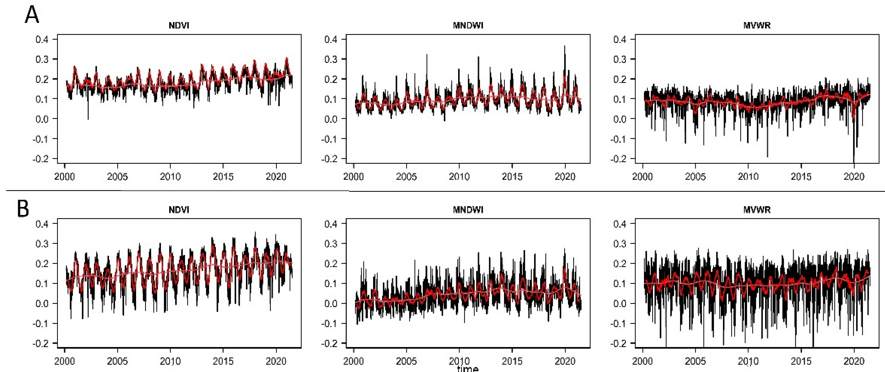
Figure 5.
Early warning signals analysis using time series of remotely sensed indices. The first column represents Normalized Difference Vegetation Index (NDVI), the second column represents Modified Normalized Water Index (MNDWI), and third column represents Modified Vegetation Water Ratio (MVWR) from February 18, 2000, to July 31, 2021, at 500-m spatial resolution in Qeshm Island (A), and Gabrik (B). The red line illustrates the rolling window size of 50 percent which was used in the analysis. The acf(1) refers to autocorrelation at lag one, SD refers to standard deviation.
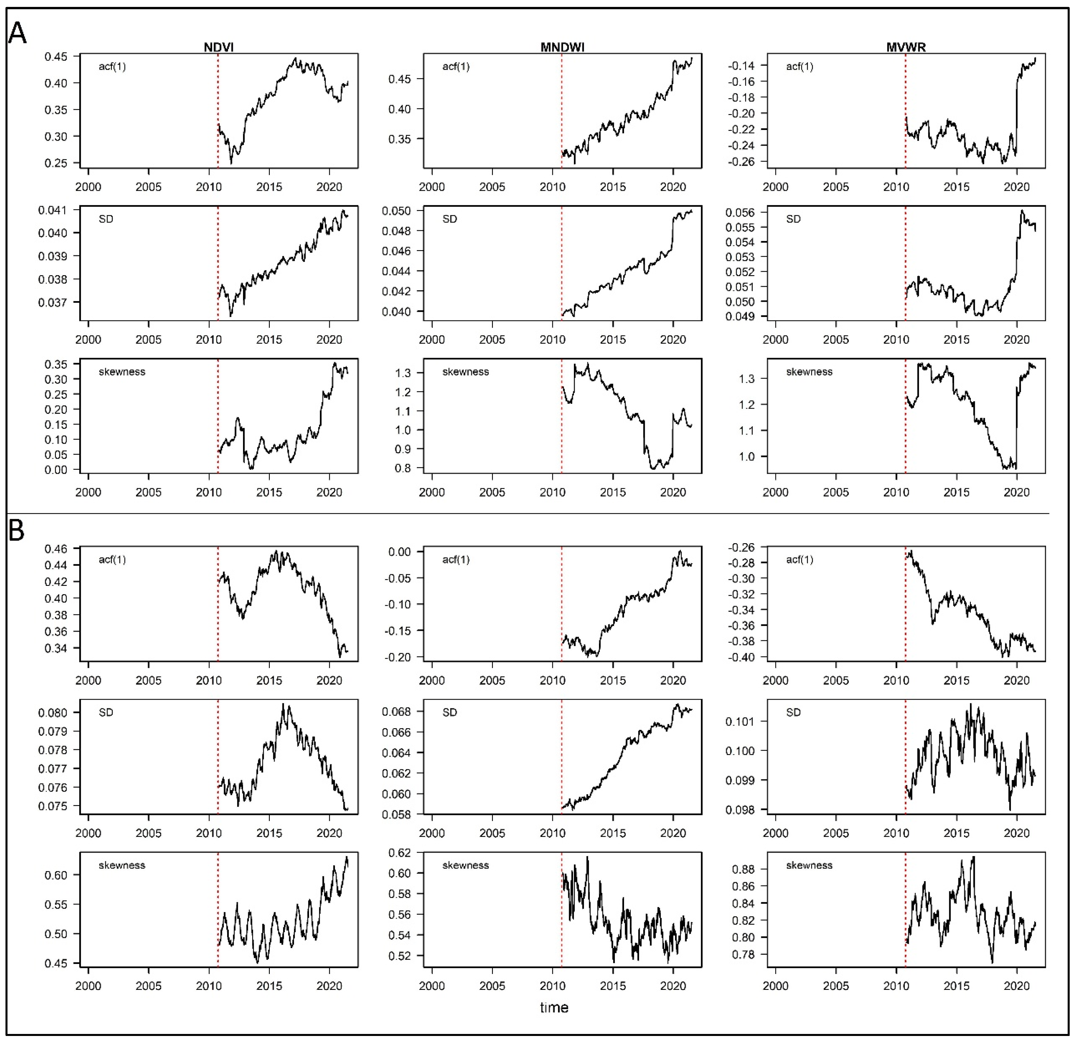

Table 1.
land-use and land cover-changein Qeshm Island and Gabrik between 1996 and 2014, obtained from Landsat data at 30-m spatial resolution.
Table 1.
land-use and land cover-changein Qeshm Island and Gabrik between 1996 and 2014, obtained from Landsat data at 30-m spatial resolution.
| Case study | Class | 1996 (number of pixels) | 2014 (number of pixels) | Change (number of pixels) | Percentage (%) |
|---|---|---|---|---|---|
| Qeshm | Agriculture | 51615 | 51953 | 338 | 0.65% |
| Bare-land | 1571765 | 1514405 | -57360 | -3.65% | |
| Built-up | 55525 | 91284 | 35759 | 64.40% | |
| Mangrove | 66672 | 73552 | 6049 | 9.07% | |
| Vegetation | 9787 | 15836 | 6880 | 70.30% | |
| Water-body | 1012778 | 1021114 | 8336 | 0.82% | |
| Gabrik | Agriculture | 30929 | 35637 | 4708 | 15.22% |
| Bare-land | 1674507 | 1665878 | -8629 | -0.52% | |
| Built-up | 5317 | 5532 | 215 | 4.04% | |
| Mangrove | 8342 | 9132 | 790 | 9.47% | |
| Vegetation | 81579 | 84207 | 2628 | 3.22% | |
| Water-body | 657401 | 657689 | 288 | 0.04% |
Table 2.
Kendall’s τ trend of autocorrelation, standard deviation, and skewness in Qeshm Island and Gabrik (significant at P < 0.1) of Normalized Difference Vegetation Index (NDVI), Modified Normalized Water Index (MNDWI), and Modified Vegetation Water Ratio (MVWR) from February 18, 2000, to July 31, 2021.
| Statistical Measures | Qeshm | Gabrik | ||||
|---|---|---|---|---|---|---|
| NDVI | MNDWI | MVWR | NDVI | MNDWI | MVWR | |
| Autocorrelation | 0.411 | 0.817 | 0.181 | 0.037 | -0.046 | 0.004 |
| Standard Deviation | 0.535 | 0.827 | -0.207 | -0.689 | 0.652 | -0.483 |
| Skewness | 0.631 | 0.401 | -0.271 | -0.199 | -0.191 | 0.07 |
Disclaimer/Publisher’s Note: The statements, opinions and data contained in all publications are solely those of the individual author(s) and contributor(s) and not of MDPI and/or the editor(s). MDPI and/or the editor(s) disclaim responsibility for any injury to people or property resulting from any ideas, methods, instructions or products referred to in the content. |
© 2023 by the authors. Licensee MDPI, Basel, Switzerland. This article is an open access article distributed under the terms and conditions of the Creative Commons Attribution (CC BY) license (http://creativecommons.org/licenses/by/4.0/).
Copyright: This open access article is published under a Creative Commons CC BY 4.0 license, which permit the free download, distribution, and reuse, provided that the author and preprint are cited in any reuse.


