
Submitted:
11 October 2023
Posted:
13 October 2023
You are already at the latest version
Abstract
Mechanical engineering plays an important role in the design and manufacture of medical devices, implants, prostheses, and other medical equipment, where the machining of bio-compatible materials have a special place. There are a lot of different conventional and non-conventional types of machining of biocompatible materials. One of the most frequently used methods is milling. The first part of this paper considers the optimization of machining parameters for minimizing surface roughness in milling biocompatible alloy Ti-6Al-4V. With four factors (cutting speed, feed rate, depth of cut, and cooling/lubricating method), each having three levels, the full factorial design implies 81 experiments have to be carried out. Using the Taguchi method, the experiment number was reduced from 81 to 27 runs through an orthogonal design. According to the analysis of variance (ANOVA), the most significant parameter for surface roughness is feed rate. In the second part possibilities of different ML techniques to create a predictive model for average surface roughness using previously created small dataset are explored. Several ML technologies and techniques that can deal successfully with small dataset were explored. The best results show commonly used machine learning algorithm Random Forest that is widely used in regression problems.
Keywords:
surface roughness
; biocompatible materials
; alloy
; Ti-6Al-4V
; Taguchi method
; ANOVA
; neural networks
; Random Forest
1. Introduction
Mechanical engineering plays an important role in the design and manufacture of medical devices, implants, prostheses, and other medical equipment, where the machining of bio-compatible materials have a special place [1,2]. Biocompatible materials are materials that are acceptable for use in contact with biological tissue, such as human skin, muscles, bones, or organs. After being integrated into the body, they do not cause rejection or damage to the surrounding tissue or other harmful effects on the body. Biocompatible materials are used in medicine to make implants, prostheses, surgical sutures, and other medical devices. There are many types of biocompatible materials, and some of them are [3,4]:
- Polymers (polyurethanes, polycarbonates, and polyesters);
- Ceramic materials;
- Metals (titanium, cobalt, chromium and their alloys, as well as stainless steels);
- Biological materials (collagen, hyaluronic acid, and fibrin);
- Composites;
- Nanomaterials.
There are a lot of different conventional and non-conventional types of machining of biocompatible materials. The most commonly used conventional machining types are milling, turning, and drilling, while the most commonly used non-conventional machining types are abrasive jet machining, ultrasonic machining, dry ice machining, laser beam machining, electrical discharge machining (EDM), and electron beam machining [5]. This paper analyses the machining of the biocompatible material titanium alloy Ti-6Al-4V (titanium alloy). Alloy Ti-6Al-4V belongs to the group of alloys, i.e. difficult-to-machine (DTM) materials. Namely, high strength and low thermal conductivity make it difficult to machine this alloy. Implants made of Ti-6Al-4V are used for making endoprostheses, dental implants in dentistry, and surgical tools. Apart from biomedicine, this alloy is often used in the aviation industry due to its high strength, corrosion resistance, and low specific gravity [6].
2. Literature review
Milling is very common conventional machining type of this material. This paper analysis effects of machining parameters (cutting speed, feed rate, depth of cut) and cooling/lubricating on surface roughness on Ti-6Al-4V alloy milling.
Optimizing cutting parameters is crucial to achieve efficient material removal rate, prolong tool life, and have better surface quality, i.e. lower average surface roughness (Ra). Optimal cutting parameters can vary based on different factors, like the machine tool, tool holder, jigs and fixtures and other factors.
Cutting speed. Titanium alloys have low thermal conductivity, so it’s important to manage heat generation. Generally, moderate cutting speeds are preferred to avoid excessive tool wear. In general, tool manufacturers recommend that alloys be produced at lower cutting speeds, so recommendations are often in the range of 30 to 90 meters per minute (m/min). By reviewing the relevant literature, it can be seen that researchers use different cutting speeds for milling titanium alloys, mostly in the range of 30 m/min to 200 m/min [7,8,9,10,11,12,13,14,15,16].
Feed rate. The feed rate is very important to strike a balance between material removal rate and tool life. The relationship between maximum surface roughness and feed rate is also well known and for the straight turning using a single point cutting tool. Maximum surface roughness is directly proportional to the square of the feed rate and inversely proportional to the nose radius. Feed rate is the factor that in most cases has the greatest influence on average surface roughness (Ra) on milling titanium alloy. Lower feed rates are usually recommended for titanium alloys to reduce the risk of tool wear and tool breakage. On milling titanium alloys feed rates typically range from 0.05 to 0.15 mm/tooth [7,11,12,13].
Depth of cut. A smaller depth of cut values is often preferred on machining titanium alloys due to their low thermal conductivity. Many researchers mainly use end mill tool on milling titanium alloy, either solid end mill or end mill with inserts [7,8,9,10,11,12,13,15,16] . The surface roughness measurement is generally performed on the bottom surface. Thereby, radial depth of cut (width of cut) is around ½ end mill diameter [9,11], while axial depth of cut varies.
By reviewing the literature, it can be seen that there are a lot of researches on milling titanium alloy Ti6Al4V. Table 1 provides an overview of cutting parameters of relevant researches. By analysing this, it can be seen that there is a difference in the ranking of cutting parameters.
Cooling / lubricating technique. Since titanium alloy belongs to group of the difficult-to-cut material, cooling/lubricating method is very important and have a significant influence on tool life and surface quality. Cutting fluids provides good cooling and lubricating properties. But considering that there is significant evidence that cutting fluids has the negative impact on human health and the environment, efforts are being made to replace them with other cooling/lubricating methods [17]. Over the past few decades, novel solutions have emerged to address the primary limitations associated with cutting fluids. Principal alternatives encompass dry cutting, minimal quantity lubrication (MQL), cryogenic cooling, solid lubrication, environmentally friendly cutting fluids, and nanofluids.
Dry machining offers several potential advantages, including reduced environmental impact due to the elimination of coolant waste and reduced operational costs associated with purchasing, maintaining, and disposing of cutting fluids. Danish et al. [10] investigate machinability performance of coated carbide insert tool under dry machining on turning. They concluded that average surface roughness (Ra) has lower values at higher cutting speed and lower feed rate, but flank wear was more intensive at lower feed rate (0,1 rev/min) comparing to higher value (0.2 rev/min). Ginting et al. [11] use uncoated cemented carbide tools in ball-end milling of titanium alloy Ti6242S under dry conditions. Sun et al. [13] conduct an experiment on turning titanium alloy in dry conditions using PCD and PCBN inserts, concluded that PCBN tool life was much shorter than that of PCD tool under the same cutting conditions. Narasimhulu et al. [18] have studies machining parameters and rake angle on average surface roughness (Ra) and cutting force on turning titanium alloy. They concluded that feed and depth of cut are the most significant factors affecting cutting force, and feed and cutting velocity affecting surface roughness. The absence of cooling and lubrication can lead to higher temperatures at the cutting zone, potentially causing thermal damage to the workpiece and tool. Machining Ti6Al4V under dry conditions is possible, but it requires careful planning, selection of appropriate tools and parameters, and considerations for heat management and chip control to achieve successful results.
Minimum quantity of liquid (MQL) involves the application of a very small amount of lubricant or coolant directly to the cutting zone during machining operations. This method aims to provide the necessary lubrication and cooling to improve tool life and machining performance while minimizing the amount of lubricant used compared to traditional flood coolant systems. Iqbal et al. [8] investigate influence of the MQL and several types of cryogenic coolant and lubricant on tool wear, cutting forces, and surface roughness. They found that MQL is more effective than the LN2 and Co2 in reducing tool wear and provide better surface quality.
Cryogenic cooling as a method that involves the use of extremely low temperatures to cool the cutting tool and workpiece during machining is particularly interesting when machining challenging materials like titanium alloys such as Ti6Al4V. These coolants have extremely low temperatures and rapidly evaporate upon contact with the heat generated during machining. Cryogenic cooling rapidly removes heat from the cutting zone, reducing the risk of thermal damage to both the tool and the workpiece, significantly extend the life of cutting tools by reducing tool wear, improve surface finish due to reduced friction and heat-induced distortion, decrease cutting force. Cryogenic coolants are environmentally friendly because they evaporate quickly without leaving behind residues or generating harmful waste. Negative aspects on using this technology are related to costs, since it can be expensive to set up and maintain due to the need for specialized equipment and cryogenic fluids, needs for careful adjustment of coolant flow rates and finally extremely low temperatures can make some materials, including certain tool materials, more brittle. Many researchers investigate the effects of cryogenic cooling on milling titanium alloys. Jerold et al. [19] investigate influence of cryogenic coolants LN2 end CO2 in machining of Ti-6Al—4V and how it effects on surface roughness, cutting temperature, tool wear and cutting forces. Cryogenic cooling decrease significantly cutting force and cutting temperature comparing to flood machining and dry machining. At the same time, lower cutting temperatures and lower forces are achieved using LN2 than using Co2. Shokrani et al. [7] investigate effects of cryogenic cooling on surface roughness on milling Ti–6Al–4V titanium alloy. They reported that with cryogenic cooling surface roughness is 39% lower comparing to dry cutting and 31% comparing to flood cooling. Xiufang et al. [16] evaluate the lubrication performances of different nanofluids in milling titanium alloy Ti-6Al-4V, using following nanofluids: graphite, Al2O3, MoS2, SiC, SiO2, CNTs. They discussed effects of using nanofluids on surface roughness and milling force.
Vortex tube offers an alternative to traditional liquid coolants by providing a clean stream of air to cool cutters and workpieces during machining. The vortex tube (Ranque-Hilsch vortex tube) is a mechanical device that separates a compressed gas into two distinct streams of air, hot and cold one. The vortex tube can reduce ambient temperature by -40C, depending on air pressure supplied to the tube. This device has no moving element of external heat source to achieve temperature separation. Šterpin Valić et al. [20] investigate the influence of cooling using MQL in combination with the vortex tube on surface roughness and tool life while turning of stainless steel. Yüksel et al. [21] used a vortex tube to investigate the effects of cooling on the turning parameters. They found that lower temperature decrease surface roughness significantly, while influence on cutting force is negligible. Singh et al. [22] use vortex tube implemented into the MQL in turning titanium alloy grade 2. The research is focused on the average surface roughness, power consumption, cutting force and tool flank wear. The authors reported that this technology (VMQL) reduced surface roughness 15% -18% comparing to MQL, and also reduction in cutting force achieved.
In metal cutting, spatially difficult-to-cut materials such as Ti6Al4V, working with big datasets isn’t always practical. Using AI can help predict outcomes even with smaller datasets. Choosing the right AI technique is very important, as there are many options to consider. Recently, applying AI techniques in metal cutting for various output factors like average surface roughness and cutting forces has become an appealing and active area of interest. Particularly interesting is the utilization of small datasets, which is common in metal cutting due to the challenges of numerous and costly experiments. Several suthors [27,28,29,30,31,32,33] employed neural networks, featuring either one or two hidden layers, in order to predict surface roughness using a relatively small dataset of 27 samples. They experiment by adjusting the number of hidden layers, varying the number of neurons within those layers, and employing different training algorithms to identify the neural network configuration that yielded the best performance.
Some researchers, like Kosarac et al., [31] leverage neural networks and relatively small datasets to predict various phenomena beyond surface roughness. They employed an Artificial Neural Network (ANN) model to analyze how working conditions influence the thermal behavior of a motorized grinder spindle. Their investigation focused on four key factors: the number of revolutions, motor coolant flow, bearing coolant flow, and the type of coolant. The dataset comprised 40 sets of data. Their findings revealed that the 4-8-8-3 network topology exhibited the lowest Root Mean Square Error (RMSE) value, signifying that this particular model demonstrated the most outstanding performance.
Dubey et al. [32] conducted an experiment focusing on surface roughness in the machining of AISI 304 Steel. The experiment consisted of 27 samples, each involving various combinations of input parameters: depth of cut, feed rate, cutting speed, and nanofluid concentration. On the base of the experimental data, Dubey developed three machine learning models to predict surface roughness based on the input parameters: Linear Regression (LR), Random Forest (RF), and Support Vector Machine (SVM). It was revealed that the Random Forest (RF) model outperformed the other two models in predicting surface roughness accurately.
Agrawal et al. [33] conducted an experiment involving AISI 4340 steel, where they varied the depth of cut, feed rate, cutting speed, and measured surface roughness. They collected a dataset consisting of 39 samples and developed three regression models: Multiple regression, Random forest, and Quantile regression. The results of the study led to the conclusion that the Random Forest regression model outperformed the other models in predicting surface roughness.
This suggests that Random Forest regression may be the superior choice for predicting surface roughness in such kind of problems
3. Exprerimental setup
This study explores the impact of four variables on surface roughness: cutting speeds (v), feed rate (f), axial depth of cut (a), and the various types of coolants/lubricants, each with three distinct levels. All experimental trials were conducted under uniform machining conditions and on the same machine tool. Experiments were conducted using the milling center Emco Concept Mill 250. Spindle milling cutter HF 16E2R030A16-SBN10-C PRAMET which utilizes two of BNGX 10T308SR-MM: M8345 inserts for superalloy cutting was used for the experiment. The arithmetic mean roughness Ra was measured by a Mitutoyo SJ-210 measuring device, Figure 1 . For this experiment, measuring parameters are set according to the expected value of the Ra to f = 2.5 m, c = 0.8 mm , ln = 4 mm. After machining three measurements of the workpiece are performed (one measurement at three different positions). The workpeace from superalloy Ti-6Al-4V with dimensions of 35 × 25 × 20, were clamped using a versatile milling vise in the machining process. This machining operation involved both sides of the sample parts and employed the climb milling method. This approach was chosen to enhance the quality of the machined surface.
The chemical composition of Ti-6Al-4V super alloy is given in Table 2.
The selection of cutting parameter levels was established by considering the recommendations from the tool manufacturer, which were aligned with the characteristics of both the workpiece and the tool material. Also, machining parameters used in research systematized in Table 1, played an role in demanding range of factors. The factors and their levels are shown in Table 3.
The rpm values used in the experiment (n1 = 1000 rpm, n2 = 2000 rpm, and n3 = 3000 rpm) were calculated based on adopted upper and lower cutting speeds (Table 3).
where D is the cutter diameter, and v cutting speed.
The feed rate per minute is calculated using the determined rpm, feed per tooth value (Table 3), and number of inserts of the cutting tool. The minimum feed rate corresponds to the smallest number of revolutions ( = 1000 rpm) and the lowest value of feed per tooth ( = 0.05 mm/tooth). The maximum feed rate ( = 1200 mm/min) corresponds to a maximum rpm ( = 3000 rpm) and maximum feed per tooth ( = 0.2 mm/tooth).
where is calculated spindle speed, feed per tooth, and z number of inserts in the cutting tool. The axial depth of the cut had value of a = 0.5, 0.8, and 1.2 mm, while the radial depth of the cut is constant for all experimental runs and equal to one-a-half of tool diameter, i.e. 8 mm. The following cooling/lubricating methods were used: emulsion, dry cutting, and vortex tube, Figure 2. For wet machining semi-synthetic fluid BIOL MIN-E, a level of quality ISO 6743/7 has been used. The vortex tube, also known as the Ranque-Hilsch vortex tube, is a mechanical device that can separate compressed gas into hot and cold streams without the need for any moving parts, Figure 2. Easy to mount with a magnetic base and flexible hose, the vortex tube creates instant cold air by reducing ambient air temperatures down by .
4. Optimizing cutting parameters using the Taguchi method
The impact of various factors on surface quality was assessed through experimentation. While a full factorial plan necessitates conducting the maximum number of experimental runs, contingent upon the factors and their levels, this can lead to increased time and experimental costs. In contrast, the Taguchi method, a widely adopted approach in experimental design, allows for a reduced number of experimental runs compared to the full factorial plan. The primary objective of the Taguchi method is to determine the minimum number of experimental runs required to identify the optimal combination of factors and their respective levels. Subsequent data analysis is conducted using statistical methods. The Taguchi optimization method is applied to attain low surface roughness in various cutting operations, as evidenced by references [9,14,23,24,26]. Furthermore, the signal-to-noise ratio, serving as a metric for assessing quality characteristics, is closely monitored. This ratio quantifies the deviation from the desired value. In the context of addressing static problems, three common signal-to-noise ratios are utilized: "smaller is better," "bigger is better," and "nominal is the best." In this particular experiment, the objective was to determine the arithmetic mean roughness (Ra), with a focus on the "Smaller is better" criterion for the selected S/N ratio of interest.
In the provided equation, S/N represents the signal-to-noise ratio, ’n’ signifies the number of responses, and ’yi’ denotes the response associated with a specific factor/level combination. In this scenario, a complete factorial experiment involved a total of experimental runs. By implementing the Taguchi method, the number of experiments was streamlined from 81 runs down to 27 runs through the use of an orthogonal design. The orthogonal matrix, as depicted in Table 4, consists of 27 rows, corresponding to the number of conducted experimental runs.
The last column in Table 4 contains S/N values derived from measuring Ra values, using the "Smaller is better" criterion outlined in Equation (Section 4). These S/N values are instrumental in identifying the most influential parameters in relation to the arithmetic mean roughness, Ra. An aggregated S/N ratio for the arithmetic mean roughness (Ra) across all factors was computed and is presented in Table 4 . A higher S/N value indicates better performance. The optimal setting for the arithmetic mean roughness Ra corresponds to the highest S/N value, which was achieved when using a cutting speed of 50 m/min (level 1), a feed rate of 0.05 mm/tooth (level 1), an axial depth of cut of 0.5 mm (level 1), and machining with emulsion (level 1) as depicted in Figure 3 and Table 5. It’s worth noting that the feed rate had a more pronounced impact on the arithmetic mean roughness, Ra, compared to cutting speed, depth of cut, and the choice of cooling/lubrication techniques, which exhibited relatively less influence. Optimization based on the "Smaller is better" criterion led to the identification of the optimal combination, coded as 1-1-1-1. This signifies the following input parameters: cutting speed of 50 m/min, feed rate of 0.05 mm/tooth, depth of cut of 0.5 mm, and machining with emulsion (Table 6 ) .
Since the 1-1-1-1 combination does exist in the orthogonal array, a confirmation experiment do not need to be conducted. Combination 1-1-1-1 has minimal values Ra = 0.194 m.
5. Analysis of variance (ANOVA)
Analysis of variance (ANOVA), as a statistical technique, was used to test the significance of the main factors compared to a mean square. A goal of the ANOVA is to estimate the experimental flaw at a certain level of confidence. In this paper, the arithmetic mean roughness (Ra), which was obtained experimentally, has been analyzed by ANOVA. ANOVA illustrates the degree of importance for each of the four factors that influenced the arithmetic mean roughness (Ra). Table 7 shows the results of the ANOVA for the arithmetic mean roughness (Ra).
The magnitude of the F-test (depth of cut) is found to be less than 1, suggesting that this particular value holds limited significance. Consequently, the consideration of factor C is reassessed, and upon its exclusion, the F-test value is recalculated, table 7.
Columns 5 and 6 in Table 8 present the significance levels of the process parameters concerning the arithmetic mean roughness Ra, indicating whether the factors had a discernible impact on Ra. According to the F distribution tables, the thresholds for significance at 95% and 99% confidence levels are as follows: F0.05, 2.20 = 3.49, and F0.01,2.20 = 5.848. That means that only one factor, feed rate, presents physical and statistical significance corresponding to 95% and 99% confidence levels since F > F = 5% and F > F = 1% for that factor. Factor A, cutting speed, presents physical and statistical significance corresponding to 95%, but not to 99% confidence. Colling lubricating technique shows physical and statistical insignificance for a confidence level of 95%, and therefore for a confidence level of 99%. Extensive research has consistently demonstrated that the feed rate stands out as the most impactful factor, showing the strongest influence on determining the arithmetic mean roughness (Ra) [7,11,14,15].
6. Machine learning (ML) approach to predict surface roughness in milling
In the field of ML, working with small datasets can be challenging. Many ML models require large amounts of data for effective training. However, there are several ML algorithms that can deal successfully with small datasets. The required size of a dataset for training an ML model can vary widely depending on several factors, the complexity of the problem, and the specific requirements of the model. There is no fixed threshold for the "ideal" dataset size, but here are some general guidelines for different ML algorithms. This study conducts a comparative analysis employing various machine learning algorithms to predict surface roughness in milling using regression techniques. Each of these algorithms has its strengths and weaknesses, making them suitable for different types of data and problem scenarios. Considering the specific characteristics of the dataset, which consists of a modest 27 samples and involves a regression task with 4 input features and 1 output, the following machine learning approaches can be taken into consideration.
Neural Networks often requires substantial amounts of data, but can still be effective with small datasets. Regularization techniques can help prevent overfitting.
Decision trees can work well with small datasets because they partition the data into subsets based on simple rules. They are less likely to over fit, making them suitable for limited data.
Random forests build multiple decision trees and aggregate their predictions, improving accuracy and reducing overfitting. This ensemble approach is effective with small datasets.
Linear regression can be effective when there are clear linear relationships between input and output. It’s relatively simple and less prone to overfitting with small datasets.
K-Nearest Neighbors (KNN) makes predictions based on nearby data points. With small datasets, it identify meaningful neighbors, leading to accurate predictions.
Ridge, Lasso, and Elastic Net Regression regularization techniques can prevent overfitting by introducing penalty terms into the regression process, which is particularly beneficial when data is scarce.
Support Vector Machine (SVM) Regression aims to find the best-fitting hyperplane. With a small dataset, SVM can still find a well-defined boundary between classes, avoiding overfitting.
Gradient boosting builds models sequentially, focusing on data points that were previously mispredicted. This targeted learning from limited data can lead to strong predictive performance.
Above mentioned techniques are less prone to over-fitting and that can effectively handle the limited data. The appropriateness of each algorithm hinges on the distinct attributes of the dataset and the inherent relationships among variables. This paper will assess each of the aforementioned algorithms, and through an analysis of their performances, the most suitable choice for a small dataset will be ascertained. Evaluating of the model performances quality involve various metrics that assess its performance and capabilities. To evaluate and access the quality of neural networks for regression tasks the most often used are:
- Mean Squared Error (MSE) and Mean Absolute Error (MAE), as a measure the magnitude of prediction errors;
- R-squared (Coefficient of Determination, that indicates the proportion of variance in the dependent variable that’s predictable from the independent variables;
Both R-squared (R2) and Mean Squared Error (MSE) are important metrics for evaluating the performance of regression models, but they provide different insights. R-squared measures the proportion of the variance in the dependent variable (target) that is predictable from the independent variables (features). It gives an indication of how well the model’s predictions match the actual values. A higher R-squared value indicates a better fit of the model to the data. MSE measures the average squared difference between the predicted values and the actual values. It quantifies the average magnitude of errors, with smaller values indicating better performance. MSE provides a direct measure of the quality of predictions in terms of their proximity to the actual values. In terms of evaluation, it’s generally a good practice to consider both R-squared and MSE together to get a comprehensive understanding of the model’s performance: Ideally, a good model should have both a low MSE and a high R-squared value. In practice, it’s common to consider both metrics and potentially other relevant metrics depending on the context of the problem.
The dataset utilized to train and evaluate the neural network model consists of 27 samples, which were generated through an experiment conducted using a Taguchi-designed experimental plan, Table 4. Notably, the training phase engaged 80% of these samples, equating to 21 instances for training, while the remaining 6 samples were reserved for testing and validation.
Diverse random states result in different sets of samples being used for training and testing, which in turn can lead to a range of performances of the neural network. This is why an iterative approach is employed, testing multiple seeds through a loop to observe the best network performance, including metrics like MSE and R-squared.
Consequently, the neural network that demonstrates the most optimal performance, as indicated by the highest R-squared value and the lowest MSE, is chosen for further testing and analysis.
To enhance the assessment of the neural network’s performance, an additional experiment was carried out involving a dataset comprising 12 distinct sets, Table 9 .
This particular dataset was deliberately excluded from the network’s training, testing, and validation stages. Its purpose lies in its utilization for simulating the models. As a result, the subsequent evaluation of these simulations will be visually showcased through graphical charts that display the Mean Squared Error (MSE) and R-squared (R2) values.
Cooling lubricating techniques encompass various methods such as emulsion, dry, and vortex tube. To make these descriptions usable for machine learning, the get_dummies function is employed, Table 10. This function transforms the textual representations of these techniques into numerical codes, allowing categorical variables to be represented as binary values. This enables these techniques to be utilized as input features for machine learning algorithms, enhancing the overall predictive capability of the models.
7. Deep Neural Network Evaluation - model Performance Visualization and Validation Loss
Deep neural networks can be both powerful and challenging to use with small datasets. While deep neural networks have the potential to extract valuable insights from small datasets, they also require careful consideration of overfitting and the appropriate use of regularization and hyper parameter tuning.
Constructing a robust machine learning model entails, a two-step process. Initially, it demands the provisioning of an initial dataset for training, which serves as the foundation upon which the model acquires its knowledge. Subsequently, the model’s capabilities are assessed by exposing it to previously unseen data, thereby evaluating its performance.
This paper shows examination and comparison of the effects of two specific cross-validation techniques on model performance:
- 1.
- Holdout Cross-Validation Technique: This approach involves partitioning the dataset into two distinct subsets: one for training and the other for validation. The model is trained on the training set, and its performance is subsequently assessed on the validation set. This technique is known for its simplicity and speed, making it a common choice for initial model assessment.
- 2.
- KFold Cross-Validation Technique: In contrast, KFold cross-validation method involves dividing the dataset into ’K’ equally sized subsets or "folds." The model is trained ’K’ times, each time using a different fold for validation and the remaining folds for training. This process is repeated ’K’ times, ensuring that each fold serves as the validation set once. The results are averaged to provide a robust assessment of the model’s performance. KFold cross-validation is especially useful for assessing a model’s consistency and reducing the risk of overfitting.
The choice between these cross-validation techniques can significantly impact the performance and reliability of a machine learning model, and this paper aims to compare effects of Holdout and KFold techniques on model outcomes. Table 11 and Table 12 show tested neural networks topologies. All neural network architecture comprises one or two hidden layers, trained using the Adam optimization algorithm. The learning rate, set at 0.001, guides the network’s parameter updates. Each hidden layer is composed of 8, 10 or 12 neurons, and the ReLU activation function facilitates the network’s nonlinear transformations and feature extraction. As evident from Table 11 and Table 12 , holdout cross-validation provided a clearer indication of the network’s performance on the test dataset. The 4-12-1 neural network topology with holdout cross-validation appears to be the best-performing model for existing dataset in terms of R-squared and MSE on the test dataset. KFold cross-validation results varied depending on the number of folds, making it important to choose an appropriate number of folds based on specific needs. Additionally, the performance on the simulation dataset may indicate overfitting, so further analysis and regularization techniques may be necessary to improve generalization. However, it’s essential to consider the application and significance of these metrics in the specific problem domain. In summary, while holdout cross-validation provided more consistent and interpretable results, KFold cross-validation can be useful for assessing model stability and generalization across different subsets of the data. The choice between the two techniques should depend on specific goals and the trade-offs between model performance and computational resources.
The neural network configuration is visually illustrated in Figure 4. This depiction provides insights into the specific architectural topology employed.
Figure 5 displays an actual vs. predicted values diagram generated by a neural network (NN) for testing dataset. This type of diagram typically consists of scatter points that represent the true (actual) values on one axis and the predicted values on the other axis. Each point corresponds to a data instance, where its position on the graph indicates how close the predicted value is to the actual value. The ideal scenario would be a diagonal line (y = x), indicating perfect predictions where all points lie on that line. In this case, the coefficient of determination (R-squared) for the data in Figure 5 is 0.9710 indicating that approximately 97.1% of the variability in the actual values can be explained by the predicted values from the deep neural network. Figure 6 displays the trend of validation loss over the course of training the deep neural network. The Mean Squared Error (MSE) for this model is calculated to be 0.0071, indicating how much the predicted values deviate, on average, from the actual values in the validation dataset. The validation loss curve in Figure 6 starts at the beginning of training and is observed up to the point of 661 epochs. Despite setting a total of 2000 epochs for training, an early stop function was employed, which halted the training process when the validation loss no longer significantly improved. This technique helps prevent overfitting and ensures that the model’s generalization ability is not compromised.
In this case, with early stopping, the training was stopped at the 661th epoch, suggesting that the model achieved a good balance between capturing patterns and avoiding overfitting. An MSE of 0.0071 indicates that, on average, the squared difference between the predicted and actual values is quite low, suggesting that the model’s predictions are relatively close to the true values in the validation dataset. This, combined with the use of early stopping, demonstrates a well-regulated training process that helps produce a model with strong generalization capabilities.
Figure 7 showcases the performance of the deep neural network model on a previously unseen dataset through a diagram depicting actual vs. predicted values. The model’s Mean Squared Error (MSE) is calculated to be 0.073, indicating a relatively moderate level of prediction accuracy. The R-squared value of 0.6767 suggests that approximately 67.67% of the variability in the actual values is explained by the model’s predictions. While the model’s performance is not as strong as during training and validation phases, it still demonstrates a reasonable ability to capture patterns in new, unseen data.
8. Comparative evaluation of performances: Regression algorithms analysis
Having in mind that the best model was found through a loop, aiming for a minimum MSE and maximum R-squared, and dealing with variability in model performance between runs, as well as experimenting with various training processes, layer configurations, and optimization methods, it’s indeed a complex and iterative process. Exploring alternative algorithms or methodologies is a natural step when confronted with challenges like these. While deep neural networks have shown great promise in various domains, they’re not always the best fit for every problem.
Figure 8 provides a comparative view of actual vs. predicted values for a range of commonly used regression algorithms, each designed to address overfitting concerns. Through an iterative process, including training loops, the best-performing models were selected. Among these models, the Best Random Forest algorithm stands out with a low Mean Squared Error (MSE) of 0.0007, indicative of precise predictions, and a high R-squared value of 0.9958, showcasing a robust explanation of the variance in the data. This highlights the effectiveness of the Random Forest method in capturing complex relationships within the dataset while resisting overfitting. Other algorithms also display varying levels of performance, underlining the importance of method selection based on specific problem characteristics.
Figure 9 shows evaluation of the performance of various regression algorithms that were optimized through iterative loops. The chart bar diagram provides an visual depiction of the Mean Squared Error (MSE) and R-squared scores for each algorithm. These optimized models have been fine-tuned to strike a balance between precision and generalization, and their representation in this figure illustrates their effectiveness in addressing overfitting concerns and capturing the underlying patterns in the data.
Figure 10 shows a model’s performance by presenting a bar chart comparison of Mean Squared Error (MSE) and R-squared scores for the simulated best models. The chart provides a clear visual representation of how these models stack up against each other, shedding light on the nuances of their predictive capabilities and their capacity to explain the variability within the data.
9. Conclusions
This paper consists of two distinct parts. In the initial phase, the research focused on investigating the impact of cutting parameters and a range of factor levels on average surface roughness (Ra) during the milling process of the biocompatible titanium alloy Ti6Al4V. The considered machining parameters included cutting speed, feed rate, depth of cut, and the chosen cooling/lubricating method. The experimental design was planned using the Taguchi methodology, resulting in the execution of an experiment comprising 27 individual runs, yielding a dataset of 27 sets. The outcomes highlighted a notable influence of the feed rate, as evident from the ANOVA analysis, which indicated the relative insignificance of other factors. The dataset comprising the 27 sets from the first experiment was subsequently employed for training various neural networks in the subsequent phase.
In the second part of the research, an extensive comparative analysis was conducted to assess the performance of several neural network algorithms in addressing regression problems. This analysis unveiled the most effective models, achieved through a combination of iterative loops and model simulation on previously unseen data.
Among the array of algorithms explored, the Best Random Forest algorithm demonstrated superior performance in terms of metrics. It achieved a notably low Mean Squared Error (MSE) of 0.0007, coupled with a relatively high R-squared value of 0.9958 when tested on the dataset. Additionally, on the simulation dataset, it exhibited commendable performance with an MSE of 0.0112 and an R-squared of 0.9502. These results underscore the robustness of Random Forests in effectively addressing the challenges posed by small datasets.
On the other hand, the Neural Network showcased slightly lower performance, achieving an MSE of 0.0071 and an R-squared value of 0.9710. However, its performance on the simulation dataset was comparatively less promising, with an MSE of 0.0730 and an R-squared of 0.6767. In light of these findings, the Random Forest algorithm emerges as a preferable choice, given its more consistent and reliable performance across both datasets. This success highlights its potential as a tool for similar tasks.
The Best Gradient Boosting algorithm delivered impressive results with a low Mean Squared Error (MSE) of 0.0059, accompanied by a commendable R-squared value of 0.9631, achieved with a seed of 18. This performance on the test dataset showcases its efficacy. On the simulation dataset, it maintained its strength with an R-squared value of 0.9376 and Mean Squared Error (MSE) of 00141. Notably, this performance is right behind of the Random Forest algorithm.
While the Decision Tree and Linear Regression algorithms show respectable performance, they slightly trail behind the top-performing algorithms. In contrast, the outlook for the other algorithms appears less promising, as they have not demonstrated competitive results.
Nevertheless, it’s imperative to acknowledge that the selection of the optimal algorithm heavily depends on the specific problem context. This reminds of the importance of meticulous model selection and fine-tuning based on the inherent characteristics of the problem.
In essence, this investigation underscores the versatility of a diverse range of regression techniques, thereby serving as a guide for decision-making in the model selection and evaluation.
Author Contributions
Conceptualization, A.K. and M.Z.; methodology, A.K. and S.T; software, A.K. and S.T; validation, M.Z. and S.T. and C.M.; investigation, A.K. and C.M.; resources, C.M.; writing—original draft preparation, A.K.; writing—review and editing, M.Z. and S.T; visualization, G.O.; supervision, M.Z.; project administration, G.O.; All authors have read and agreed to the published version of the manuscript.
Conflicts of Interest
The authors declare no conflict of interest.
References
- Mihov, D. , Katerska, B.: Some biocompatible materials used in medical practice, Trakia Journal of Sciences, Vol. 8, Suppl. 2, pp 119-125, 2010.
- Kiradzhiyska,D.,D., Mantcheva,R.,D.: Overview of Biocompatible Materials and Their Use in Medicine, 34 Folia Medica I 2019, I Vol. 61 I No. 1. [CrossRef]
- Parida, P, Behera, Ajit, Mishra, S, C: Classification of Biomaterials used in Medicine, International Journal of Advances in Applied Sciences (IJAAS), Vol.1, No.3, Month 2012, pp. 31 35, 2012.
- Binyamin, G., Shafi, B.M., Mery, C.M: Biomaterials: a primer for surgeons, Seminars in Pediatric Surgery, Volume 15, Issue 4, November 2006.
- Saptaji, K., Gebremariam, M.,A., Azhari, M.A.M: Machining of biocompatible materials: a review, The International Journal of Advanced Manufacturing Technology, 2018. 006.
- Liu, Z., He, B., Lyu, T., Zou Y.: A Review on Additive Manufacturing of Titanium Alloys for Aerospace Applications: Directed Energy Deposition and Beyond Ti-6Al-4V, Processing-Microstructure-Property Relationships in Additive Manufacturing of Ti Alloys, Springer, 2021.
- Shokrani, A. , Dhokia, V., Newman, S., T.: Investigation of the effects of cryogenic machining on surface integrity in CNC end milling of Ti–6Al–4V titanium alloy, Journal of Manufacturing Processes 21, 2016, 172-179.
- Iqbal, A. , Suhaimi, H., Zhao,W., Jamil, M., Nauman, M. M.,He, N., Zaini, J.; Sustainable Milling of Ti-6Al-4V: Investigating the Effects of Milling Orientation Cutter’s Helix Angle, and Type of Cryogenic Coolant, MDPI, Metals, 2020.
- Tešić, S. , Zeljković, M., Čiča, Đ Optimizacija i ispitivanje uticaja parametara rezanja na hrapavost obrad¯ene površine pri glodanju biokompatibilne legure - Ti6Al4V, TEHNIKA-MASINSTVO 68 (2019) 5.
- Danish, N., H.D. , Musfirah, A. H.: Optimization of Cutting Parameter for Machining Ti-6Al-4V Titanium Alloy, JOURNAL OF MODERN MANUFACTURING SYSTEMS AND TECHNOLOGY (JMMST), e-ISSN: 2636-9575, VOL., ISSUE 1, 53 – 57. [CrossRef]
- Ginting, A. , Nouari, M. Experimental and numerical studies on the performance of alloyed carbide tool in dry milling of aerospace material, International Journal of Machine Tools and Manufacture 46 (2006) 758–768.
- Paschoalinoto, N., W. , Batalha, G. F., Bordinassi, E., C., Ferrer, J. A. G., de Lima Filho, A., F., de L. X. Ribeiro, G., Cardoso, C. MQL Strategies Applied in Ti-6Al-4V Alloy Milling—Comparative Analysis between Experimental Design and Artificial Neural Networks: MDPI, Materials, 2020, 2020. [Google Scholar]
- Sun, J. , Guo, Y.B. A comprehensive experimental study on surface integrity by end milling Ti–6Al–4V, Journal of Materials Processing Technology 209 (2009) 4036–4042.
- Rahman, Al Mazedur, Rob,S.,M.,A., Srivastava,A.,K. Modeling and optimization of process parameters in face milling of Ti6Al4V alloy using Taguchi and grey relational analysis, f49th SME North American Manufacturing Research Conference, NAMRC 49, Ohio, USA, Procedia Manufacturing 53 (2021) 204–212.
- Karkalos, N.E. , Galanis, N.I., Markopoulos, A.P. Surface roughness prediction for the milling of Ti–6Al–4V ELI alloy with the use of statistical and soft computing techniques, Measurement, 90 (2016), 25-35.
- Bai, X. , Li, C., Dong, L., Yin, Q. Experimental evaluation of the lubrication performances of different nanofluids for minimum quantity lubrication (MQL) in milling Ti-6Al-4V, The International Journal of Advanced Manufacturing Technology (2019) 101:2621–2632.
- Benedicto, E. , Carou, D., Rubio, E.M. Technical, Economic and Environmental Review of the Lubrication/Cooling Systems used in Machining Processes, Advances in Material and Processing Technologies Conference, Procedia Engineering 184 ( 2017 ) 99 – 116.
- Narasimhulu Andriya: Dry Machining of Ti-6Al-4V using PVD Coated TiAlN Tools, Proceedings of the World Congress on Engineering 2012 Vol III WCE 2012, July 4 - 6, 2012, London, U.K.
- Jerold, B.D. , Kumar,M.P. The Influence of Cryogenic Coolants in Machining of Ti-6Al-4V, Journal of Manufacturing Science and Engineering · May 2013,. [CrossRef]
- Šterpin Valić, G. , Kostadin, T., Cukor, G., Fabić, M. Sustainable Machining: MQL Technique Combined with the Vortex Tube Cooling When Turning Martensitic Stainless Steel X20Cr13, MDPI, Machines, 2023.
- Yüksel, S. , Onat, A. Investigation of CNC Turning Parameters by Using a Vortex Tube Cooling System, ACTA PHYSICA POLONICA A, Proceedings of the 4th International Congress APMAS2014, April 24-27, 2014, Fethiye, Turke.
- Singh, G. , Pruncu, C.,I., Gupta, M.,K., Mia, M., Khan, A.,M., Jamil, M., Pimenov, D.,Y., Sen, B., Sharma, V.S. Investigations of Machining Characteristics in the Upgraded MQL-Assisted Turning of Pure Titanium Alloys Using Evolutionary Algorithms, MDPI, Materials, 2019.
- Kosarac,A., Mladjenovic,C., Zeljkovic,M., Tabakovic,S., Knezev,M. Neural-Network-Based Approaches for Optimization of Machining Parameters Using Small Dataset, MDPI, Materials, 2022.
- Kumar, P. , Sharma, M., Singh, G., Singh, R. P. Experimental investigations of machining parameters on turning of Ti6Al4V: optimisation using Taguchi method, International Journal on Interactive Design and Manufacturing (IJIDeM), 2023.
- Beatrice, B.A.; Kirubakaran, E.; Thangaiah, P.R.J.; Wins, K.L.D. Surface roughness prediction using artificial neural network in hard turning of AISI H13 steel with minimal cutting fluid application. Procedia Eng. 2014, 97, 205–211. [Google Scholar] [CrossRef]
- Pal, S.K.; Chakraborty, D. : Surface roughness prediction in turning using artificial neural network. , Neural Comput. Appl. 2005, 14, 319–324. [Google Scholar] [CrossRef]
- Hossain, M.I.; Amin, A.N.; Patwari, A.U. Development of an artificial neural network algorithm for predicting the surface rough-ness in end milling of Inconel 718 alloy. In Proceedings of the 2008 International Conference on Computer and Communication, Engineering, Kuala Lumpur, Malaysia, 13–15 May 2008; pp. 1321–1324. [Google Scholar]
- Benardos, P.; Vosniakos, G.C. Prediction of surface roughness in CNC face milling using neural networks and Taguchi’s design of experiments. Robot, Comput.-Integr. Manuf. 2002, 18, 343–354. [Google Scholar] [CrossRef]
- Eser, A.; A¸skar Ayyıldız, E.; Ayyıldız, M.; Kara, F. Artificial intelligence-based surface roughness estimation modelling for milling of AA6061 alloy, Adv. Mater. Sci. Eng. 2021, 2021, 5576600. [Google Scholar]
- Rajesh,A. S., Prabhuswamy, M. S., Rudra Naik, M. Machine Learning Approach: Prediction of Surface Roughness in Dry Turning Inconel 625, Advances in Materials Science and Engineering, Special Issue Advanced Functional Graded Materials: Processing and Applications, 2022.
- Kosarac, A. , Cep,R., Trochta, M., Knezev,M., Zivkovic, A., Mladjenovic,C., Antic,A. Thermal Behavior Modeling Based on BP Neural Network in Keras Framework for Motorized Machine Tool Spindles, MDPI, Materials, 2022.
- Dubey. V., Sharma, A.,K., Pimenov,D.Y.: Prediction of Surface Roughness Using Machine Learning Approach in MQL Turning of AISI 304 Steel by Varying Nanoparticle Size in the Cutting Fluid, MDPI, Lubricants, 2022.
- Agrawal, A. , Goel, S., Bin Rashid, W., Price, M. Prediction of surface roughness during hard turning of AISI 4340 steel (69 HRC), Applied Soft Computing, Volume 30, May 2015, Pages 279-286.
Figure 1.
Measuring of the surface roughness.
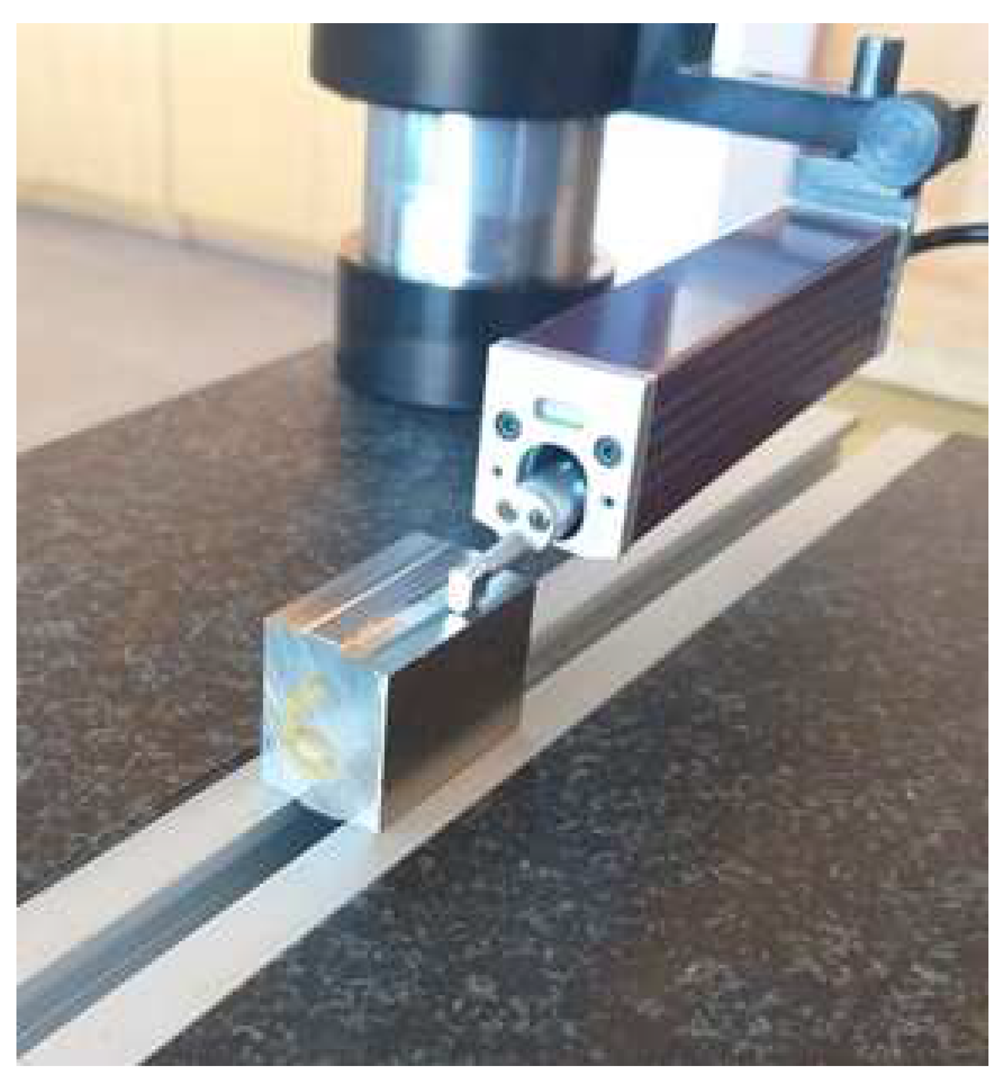
Figure 2.
Ranque-Hilsch vortex tube.
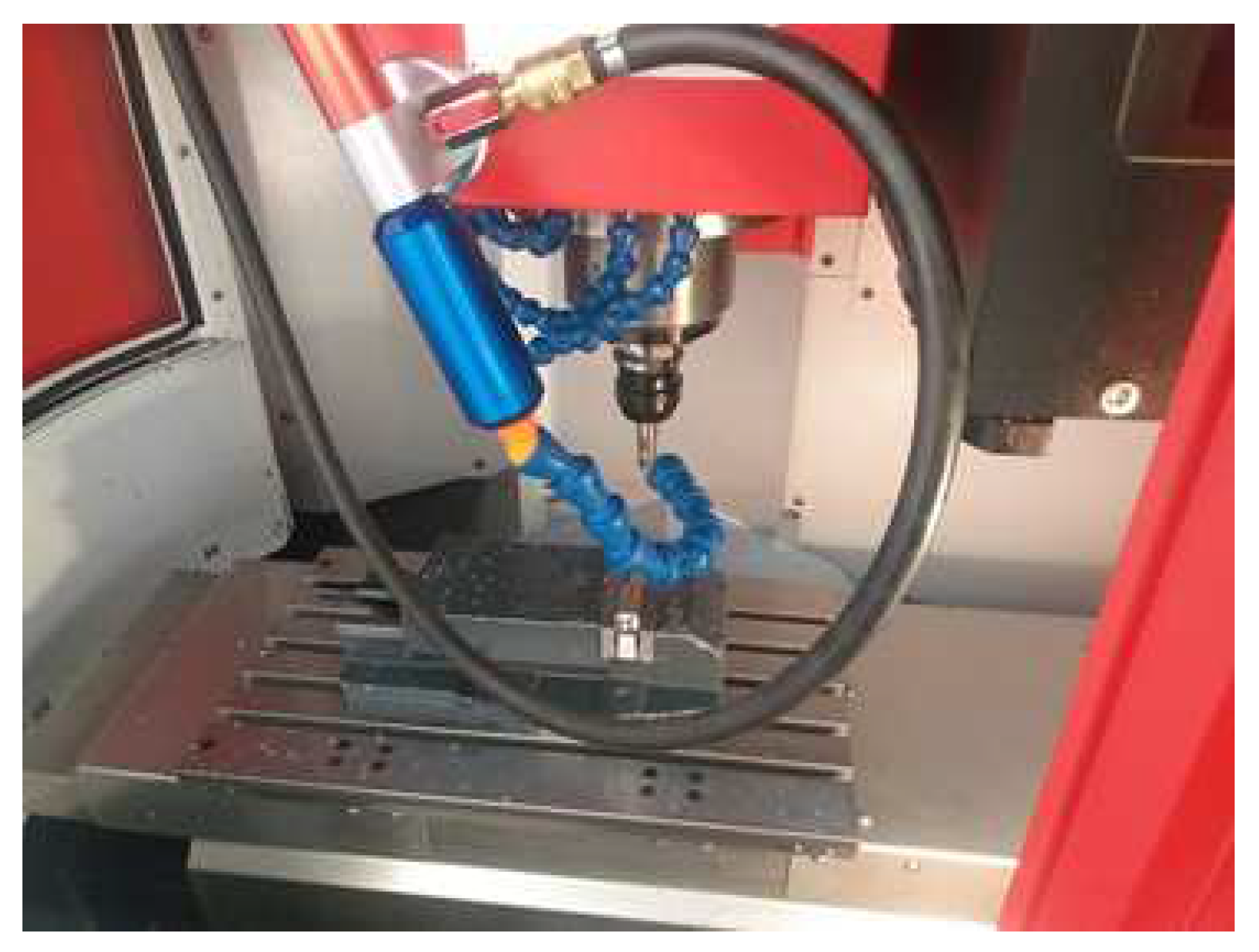
Figure 3.
Main effect plot for S/N ratio.
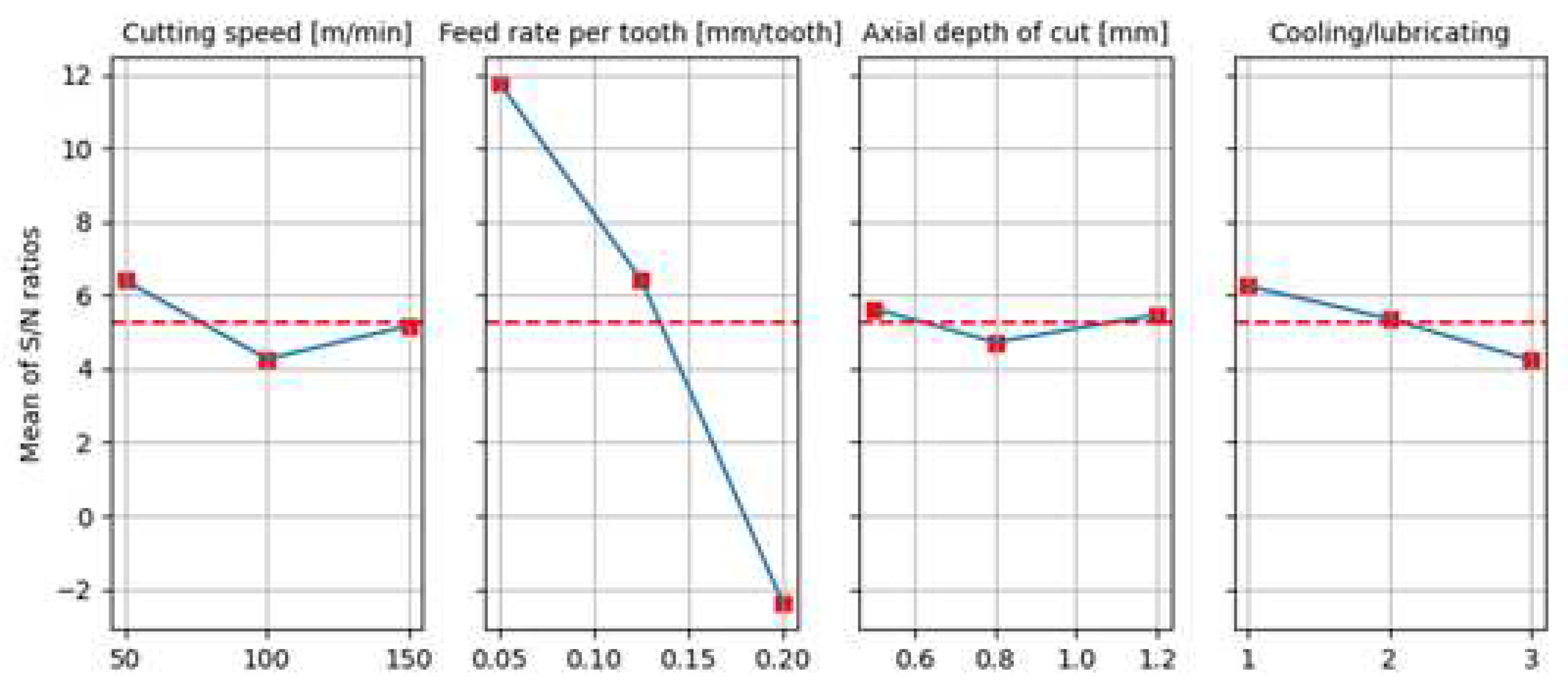
Figure 4.
Neural network topology.
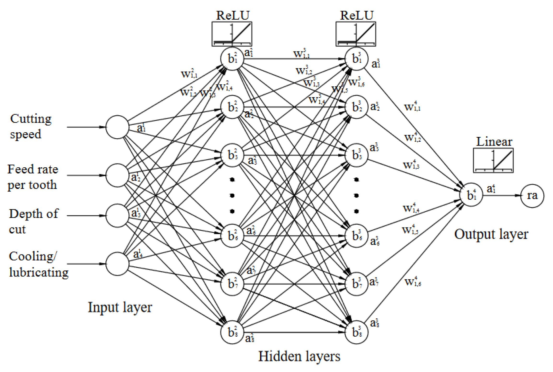
Figure 5.
Actual vs. predicted values for neural network 4-12-1.
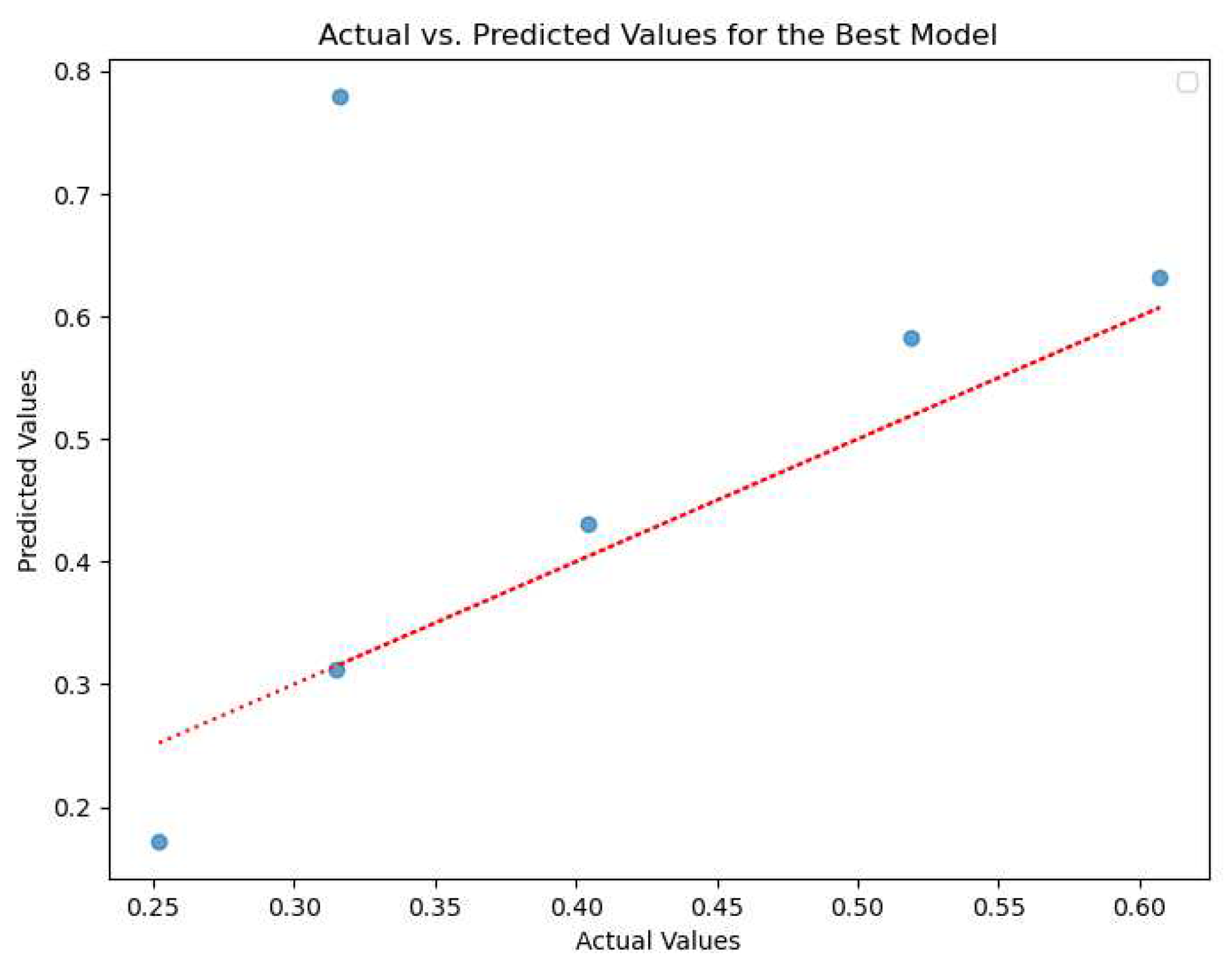
Figure 6.
Training and validation lost for neural network 4-12-1.
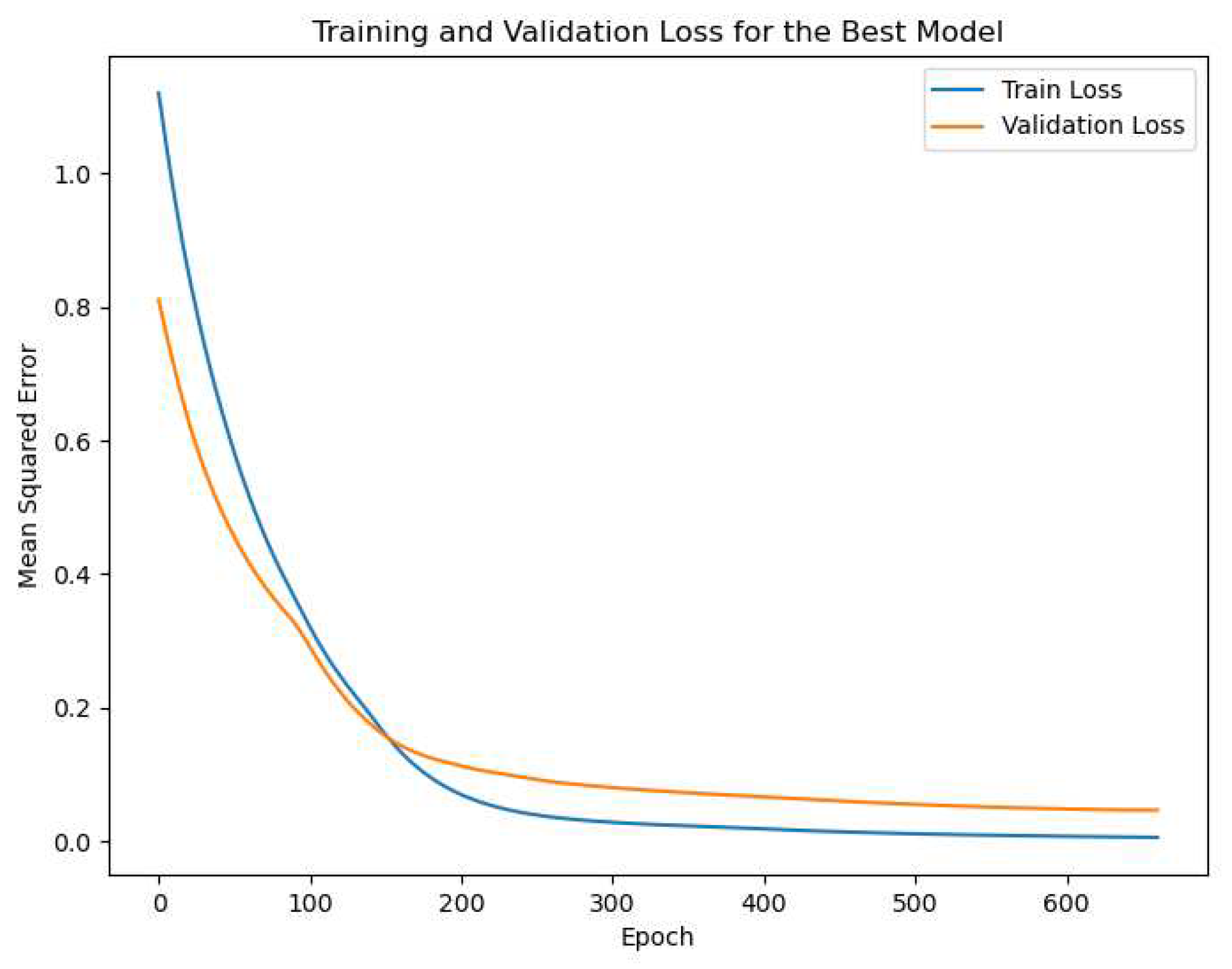
Figure 7.
Actual vs. predicted values for simulation model.
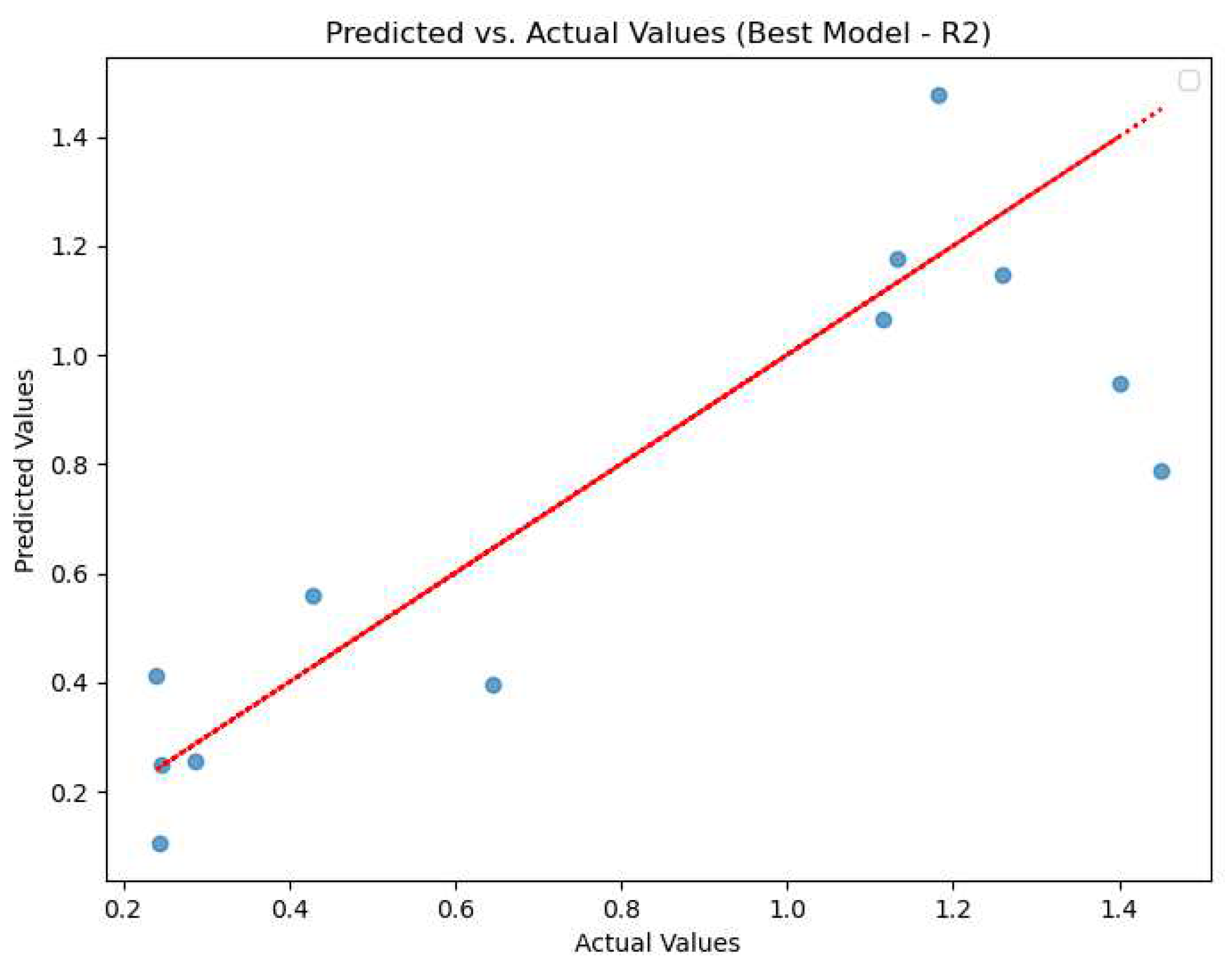
Figure 8.
Comparison of actual vs predicted values for various regression algorithms.
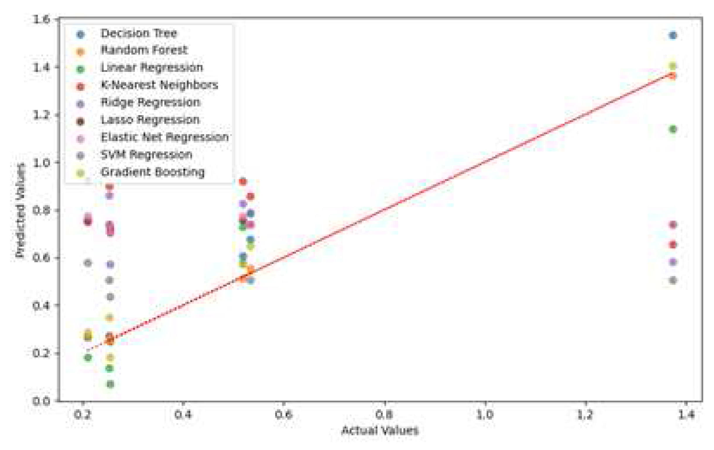
Figure 9.
A Comparative Analysis of MSE and R-squared Scores for Optimized Models Selected via Iterative Loops.
Figure 9.
A Comparative Analysis of MSE and R-squared Scores for Optimized Models Selected via Iterative Loops.
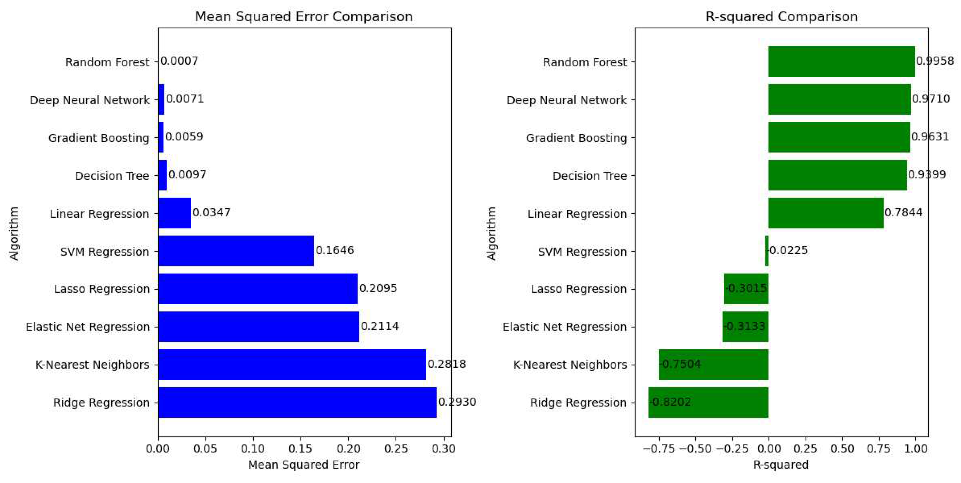
Figure 10.
Exploring Model Performance: Bar Chart Comparison of MSE and R-squared Scores for Simulated Best Models.
Figure 10.
Exploring Model Performance: Bar Chart Comparison of MSE and R-squared Scores for Simulated Best Models.
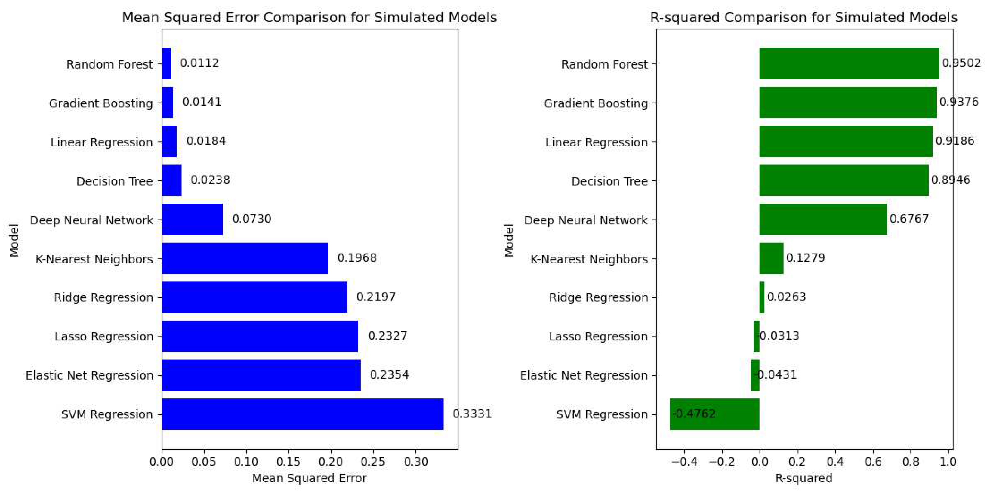

Table 1.
Prediction of the arithmetic mean roughness (Ra) in milling Ti6Al4V alloy.
| Author, Year | Process | Cutting conditions |
|---|---|---|
| Shokrani et al. (2006) [7] | Solid carbide end mill 8 | Experimental input parameters: Cutting speed 30, 115, 200 m/min, feed rate 0.03, 0.055, 0.1 mm/tooth, radial depth of cut 1, 3, 5 mm, cooling/lubricating: cryogenic, flood, dry |
| Iqbal et al. (2020) [8] | Solid carbide end mill 8 | Experimental input parameters: Cutting speed 100, 175 m/min, Cutter’s helix angle: 30, 42 deg, Milling orientation: up, down, Cutting fluid: LN2, CO2, MQL |
| Tešić et al. (2020) [9] | Indexable end mill 16 | Experimental input parameters: Cutting speed 40, 80, 160 m/min, feed rate 0.05, 0.1, 0.2 mm/tooth, radial depth of cut 8 mm, axial depth of cut 0.5, 1.0 and 2 mm |
| Danish et al. (2022) [10] | Indexable end mill | Experimental input parameters: Cutting speed 140, 150 m/min, feed rate 0.1, 0.2 mm/tooth, axial depth of cut 0.5 mm, dry cutting |
| Ginting et al. (2006) [11] | Indexable ball end mill 16 | Experimental input parameters: Cutting speed 60, 75, 100, 125, 150 m/min, feed rate 0.1, 0.15 mm/tooth, radial depth of cut 8.8 mm, axial depth of cut 2 mm, dry cutting |
| Paschoalinoto et al. (2020) [12] | Indexable end mill | Experimental input parameters: Cutting speed 80, 90, 100 m/min, feed rate 0.06, 0.08, 0.1 mm/tooth, radial depth of cut 0.5, 0.75, 1 mm, cooling / lubricating: air, MQL, MQL+graphite |
| Sun et al. (2009) [13] | Solid carbide end mill | Experimental input parameters: Cutting speed 50, 65, 80, 95, 110 m/min, feed rate 0,06, 0,08, 0.1, 0,12, 0,14 mm/tooth, radial depth of cut 2, 3, 4, 5, 6 mm, axial depth of cut 1,5 mm |
| Rahman Al Mazedur et al. (2021) [14] | Face mill | Experimental input parameters: Cutting speed 50, 57.5 65 m/min, feed rate 0.2, 0.25, 0.3 mm/tooth, radial depth of cut 7.5, 10, 12 mm, axial depth of cut 2.54 mm |
| Karkalos et al. (2016) [15] | Solid carbide end mill 6 | Experimental input parameters: Cutting speed 26.39, 32.05, 37.70 m/min, feed rate 75, 100, 125 mm/min, radial depth of cut 0.3,0.6, 0.9 |
| Bai et al. (2019) [16] | End mill | Experimental input parameters: 1200 rpm, feed rate 500 mm/min, axial depth of cut 0.25 mm, radial depth of cut 10 mm, cooling / lubricating: nanofluids |
Table 2.
The chemical composition of Ti-6Al-4 super alloy.
| V | Al | Sn | Zr | Mo | C | Si | Ti |
|---|---|---|---|---|---|---|---|
| 4.22 | 5.48 | 0.0625 | 0.0028 | 0.05 | 0.369 | 0.0222 | Balance |
Table 3.
Experimental factors and their levels.
| Factors | Levels | ||
|---|---|---|---|
| Low level | Middle level | High level | |
| -1 | 0 | 1 | |
| Cutting speed (m/min) | 50 | 100 | 150 |
| Feed rate per tooth (mm/tooth) | 0.05 | 0.125 | 0.2 |
| Axial depth of cut (mm) | 0.5 | 0.8 | 1.2 |
| Cooling / lubricating technique | Emulsion | Dry cutting | Vortex tube |
Table 4.
Experimental plan– L27 orthogonal array (Taguhci method).
| No. of Trials | Cutting Speed (m/min) | Feed per Tooth (mm/tooth) | Axial Depth of Cut (mm) | Cooling/ Lubricating Technique | Ra1 m | Ra2 m | Ra3 m | Aver. Ra m | S/N (dB) |
|---|---|---|---|---|---|---|---|---|---|
| 1 | 50 | 0.05 | 0.5 | Emulsion | 0.173 | 0.211 | 0.199 | 0.194 | 14.229 |
| 2 | 50 | 0.05 | 0.8 | Dry machining | 0.233 | 0.257 | 0.277 | 0.255 | 11.846 |
| 3 | 50 | 0.05 | 1.2 | Vortex tube | 0.234 | 0.26 | 0.254 | 0.2493 | 12.064 |
| 4 | 50 | 0.125 | 0.5 | Dry machining | 0.327 | 0.378 | 0.307 | 0.337 | 9.4388 |
| 5 | 50 | 0.125 | 0.8 | Vortex tube | 0.467 | 0.521 | 0.509 | 0.499 | 6.037 |
| 6 | 50 | 0.125 | 1.2 | Emulsion | 0.326 | 0.33 | 0.292 | 0.316 | 10.006 |
| 7 | 50 | 0.2 | 0.5 | Vortex tube | 1.345 | 1.225 | 1.32 | 1.296 | -2.256 |
| 8 | 50 | 0.2 | 0.8 | Emulsion | 1.341 | 1.315 | 1.402 | 1.352 | -2.623 |
| 9 | 50 | 0.2 | 1.2 | Dry machining | 1.225 | 1.106 | 1.094 | 1.141 | -1.150 |
| 10 | 100 | 0.05 | 0.5 | Emulsion | 0.232 | 0.278 | 0.248 | 0.252 | 11.949 |
| 11 | 100 | 0.05 | 0.8 | Dry machining | 0.286 | 0.233 | 0.297 | 0.272 | 11.308 |
| 12 | 100 | 0.05 | 1.2 | Vortex tube | 0.34 | 0.271 | 0.334 | 0.315 | 10.033 |
| 13 | 100 | 0.125 | 0.5 | Dry machining | 0.668 | 0.657 | 0.498 | 0.607 | 4.3266 |
| 14 | 100 | 0.125 | 0.8 | Vortex tube | 0.607 | 0.489 | 0.505 | 0.533 | 5.4545 |
| 15 | 100 | 0.125 | 1.2 | Emulsion | 0.446 | 0.519 | 0.602 | 0.522 | 5.6410 |
| 16 | 100 | 0.2 | 0.5 | Vortex tube | 1.479 | 1.556 | 1.565 | 1.533 | -3.712 |
| 17 | 100 | 0.2 | 0.8 | Emulsion | 1.662 | 1.337 | 1.673 | 1.557 | -3.8476 |
| 18 | 100 | 0.2 | 1.2 | Dry machining | 1.279 | 1.272 | 1.57 | 1.373 | -2.7576 |
| 19 | 150 | 0.05 | 0.5 | Emulsion | 0.21 | 0.21 | 0.21 | 0.21 | 13.555 |
| 20 | 150 | 0.05 | 0.8 | Dry machining | 0.412 | 0.22 | 0.169 | 0.267 | 11.469 |
| 21 | 150 | 0.05 | 1.2 | Vortex tube | 0.351 | 0.36 | 0.291 | 0.334 | 9.525 |
| 22 | 150 | 0.125 | 0.5 | Emulsion | 0.494 | 0.572 | 0.491 | 0.519 | 5.696 |
| 23 | 150 | 0.125 | 0.8 | Dry machining | 0.703 | 0.707 | 0.624 | 0.678 | 3.375 |
| 24 | 150 | 0.125 | 1.2 | Vortex tube | 0.298 | 0.429 | 0.487 | 0.404 | 7.858 |
| 25 | 150 | 0.2 | 0.5 | Vortex tube | 1.492 | 1.187 | 1.317 | 1.332 | -2.490 |
| 26 | 150 | 0.2 | 0.8 | Emulsion | 0.804 | 1.194 | 1.188 | 1.062 | -0.522 |
| 27 | 150 | 0.2 | 1.2 | Dry machining | 1.168 | 1.421 | 1.176 | 1.255 | -1.972 |
Table 5.
S/N ratio of the arithmetic mean roughness Ra.
| Factors | Levels | Delta | Rank | ||
|---|---|---|---|---|---|
| 1 | 2 | 3 | |||
| Cutting speed (m/min) | 6.399* | 4.266 | 5.166 | 2.133 | 2 |
| Feed rate per tooth (mm/tooth) | 11.776* | 6.426 | -2.371 | 14.146 | 1 |
| Axial depth of cut (mm) | 5.637* | 4.722 | 5.472 | 0.915 | 4 |
| Cooling / lubricating technique | 6.249* | 5.356 | 4.226 | 2.024 | 3 |
Table 6.
ROptimum Factor Levels.
| Level | v (m/min) | sz (mm/tooth) | a (mm) | Cooling / Lubricating | Ra (measured) |
|---|---|---|---|---|---|
| 1 | 50 | 0.05 | 0.5 | Emulsion | 0.194 |
Table 7.
Results of ANOVA for the arithmetic mean roughness.
| Factor | DOF | Sum of Squares | Variance | F |
|---|---|---|---|---|
| A | 2 | 0.102 | 0.051 | 5.490 |
| B | 2 | 5.615 | 2.808 | 302.467 |
| C | 2 | 0.018 | 0.009 | 0.989 |
| D | 2 | 0.051 | 0.026 | 2.760 |
| Error | 18 | 0.17 | 0.009 | |
| Total | 26 | 5.95 |
Table 8.
Final ANOVA table.
| Factor | DOF | Sum of Squares | Variance | F | Percent |
|---|---|---|---|---|---|
| A | 2 | 0.0833 | 0.051 | 5.496 | 1.4% |
| B | 2 | 5.596 | 2.808 | 302.8 | 94% |
| D | 2 | 0.032 | 0.026 | 2.73 | 0.55% |
| Error | 20 | 0.241 | 0.00927 | 4.05% |
Table 9.
Experimental plan– L27 orthogonal array (Taguchi method).
| No. of Trials | Cutting Speed (m/min) | Feed per Tooth (mm/tooth) | Axial Depth of Cut (mm) | Cooling/ Lubricating Technique | Ra1 m | Ra2 m | Ra3 m |
|---|---|---|---|---|---|---|---|
| 1 | 50 | 0.05 | 0.5 | Vortex tube | 0.247 | 0.227 | 0.247 |
| 2 | 50 | 0.2 | 0.5 | Emulsion | 1.244 | 1.14 | 1.165 |
| 3 | 50 | 0.125 | 0.8 | Dry machining | 0.425 | 0.444 | 0.42 |
| 4 | 50 | 0.2 | 0.8 | Vortex tube | 1.38 | 1.314 | 1.509 |
| 5 | 50 | 0.2 | 1.2 | Emulsion | 1.274 | 1.233 | 1.272 |
| 6 | 100 | 0.05 | 0.5 | Dry machining | 0.227 | 0.223 | 0.279 |
| 7 | 100 | 0.2 | 0.8 | Dry machining | 1.198 | 1.13 | 1.068 |
| 8 | 100 | 0.05 | 1.2 | Emulsion | 0.22 | 0.272 | 0.248 |
| 9 | 100 | 0.2 | 1.2 | Vortex tube | 1.365 | 1.406 | 1.581 |
| 10 | 150 | 0.2 | 0.8 | Dry machining | 1.005 | 1.253 | 1.092 |
| 11 | 150 | 0.05 | 1.2 | Emulsion | 0.313 | 0.267 | 0.28 |
| 12 | 150 | 0.125 | 1.2 | Vortex tube | 0.786 | 0.555 | 0.594 |
Table 10.
Dummy variable mapping.
| v | f | a | ra | Emulsion | Dry | Vortex tube |
|---|---|---|---|---|---|---|
| 50 | 0.05 | 0.5 | 0.194 | 1 | 0 | 0 |
| 50 | 0.05 | 0.8 | 0.255 | 0 | 1 | 0 |
| 50 | 0.05 | 1.2 | 0.249 | 0 | 0 | 1 |
| 50 | 0.125 | 0.5 | 0.337 | 0 | 1 | 0 |
Table 11.
Neural network parameters assessed on test and simulation dataset, Holdout cross - validation.
Table 11.
Neural network parameters assessed on test and simulation dataset, Holdout cross - validation.
| Network Topology | R-squared (test) | MSE (test) | R-squared (simulation) | MSE (simulation) |
|---|---|---|---|---|
| 4-8-1 | 0.9599 | 0.0093 | 0.3202 | 0.1534 |
| 4-10-1 | 0.9507 | 0.0144 | 0.2144 | 0.1773 |
| 4-12-1 | 0.9710 | 0.0071 | 0.6767 | 0.0730 |
| 4-8-8-1 | 0.9591 | 0.0058 | 0.1492 | 0.1920 |
| 4-10-10-1 | 0.9100 | 0.0186 | 0.6675 | 0.0750 |
| 4-12-12-1 | 0.8603 | 0.0310 | 0.3512 | 0.1464 |
Table 12.
Neural network parameters assessed on test and simulation dataset, KFold cross - validation.
Table 12.
Neural network parameters assessed on test and simulation dataset, KFold cross - validation.
| Network Topology (num. fold) | R-squared (test) | MSE (test) | R-squared (simulation) | MSE (simulation) |
|---|---|---|---|---|
| 4-12-1 (5) | 0.5562 | 0.0819 | 0.5229 | 0.1077 |
| 4-12-1 (10) | 0.3052 | 0.1181 | -0.4100 | 0.3182 |
| 4-12-12-1 (5) | 0.2623 | 0.1195 | 0.7444 | 0.0577 |
| 4-12-12-1 (10) | -0.5683 | 0.0803 | 0.6004 | 0.0902 |
Disclaimer/Publisher’s Note: The statements, opinions and data contained in all publications are solely those of the individual author(s) and contributor(s) and not of MDPI and/or the editor(s). MDPI and/or the editor(s) disclaim responsibility for any injury to people or property resulting from any ideas, methods, instructions or products referred to in the content. |
© 2020 by the authors. Licensee MDPI, Basel, Switzerland. This article is an open access article distributed under the terms and conditions of the Creative Commons Attribution (CC BY) license (https://creativecommons.org/licenses/by/4.0/).
Copyright: This open access article is published under a Creative Commons CC BY 4.0 license, which permit the free download, distribution, and reuse, provided that the author and preprint are cited in any reuse.


