
Submitted:
07 October 2023
Posted:
10 October 2023
You are already at the latest version
Abstract
Field electron emission, or electron tunneling through a potential barrier under the influence of a strong electrostatic field, is of broad interest to the accelerator physics community. For example, it is the source of undesirable dark currents in resonant cavities, providing a limit to high-field operation. The classical approach to field electron emission is the Fowler-Nordheim (FN) framework, which incorporates a simplified surface potential and various assumptions. Here we build a more realistic model using the potential and charge densities derived from a density-functional theory (DFT) calculation. We examine the correction factors associated with each model assumption. Compared to the FN framework, our results can be extended up to 80 GV/m, a limit that has been reached in laser-induced strong field emission scenarios.
Keywords:
field electron emission
; DFT
; Au (100)
; Fowler-Nordheim
; laser field emission
1. Introduction
Field electron emission from metals is due to electron tunneling from a metallic surface under a strong electrostatic or radio frequency (RF) field. This is to be differentiated from laser field emission, or electron emission under a strong laser field. Field electron emission induces surface breakdown in RF cavities at a surface field of 300 to 400 MV/m, which after geometric enhancement yields a local surface field up to 10 GV/m [1]. Surface breakdown is the source of undesirable dark currents from high-gradient accelerating structures, which can dissipate significant power from RF cavities containing such cathodes. Dark current also gives rise to significant pollution of the experimental environment downstream of the electron source. Modeling such dark currents, however, requires an accurate understanding of the physical and chemical defects of the emitting surface. The first step is to accurately model the emission from a one-dimensional, flat, chemically pure surface, and this is a major focus of the present paper.
In laser field emission, transient electric fields typically exceeding 10 GV/m and reaching values as large as 80 GV/m have been achieved [2,3]. For an 800 nm laser, the Keldysh parameter is valued at 0.23 [4], identifying the tunneling process as dominant compared to the multiphoton emission process. We therefore expect similarities between field electron emission and transient laser field emission in this limit.
The conventional model of field electron emission is the Fowler-Nordheim (FN) framework. It is a one-dimensional quantum mechanical model that arises from solving the time-independent Schrödinger equation (TISE). It uses the Wentzel-Kramers-Brillouin (WKB) approximation to find the electron transmission coefficient across a model potential barrier. The transmission coefficient as a function of the electron normal energy is given by , where the Gamow coefficient is , with the integration between the two classical turning points, or the boundary of the classically forbidden region of the potential. is the electron mass, is the electron potential as a function of longitudinal position and is the normal energy (total energy minus the surface-parallel kinetic energy) of the electronic state under consideration. The decay width, describing the exponential dependence of the transmission coefficient on normal energy, is defined as . A first-order Taylor expansion of around the Fermi level leads to a simple formula for the emission current density , where is the Sommerfeld’s free electron supply constant, and the subscript indicates evaluation at the Fermi level [5].
Besides the WKB approximation and first-order Taylor expansion, the FN framework typically employs two simplified potentials. One is the exact triangular (ET) potential of the form outside the surface, where is the work function, the elementary charge, the applied electric field, and the distance from the surface. It is set to some arbitrary nonpositive constant within the surface. Although the ET potential is an unrealistic model of a metal surface, it admits analytical solutions under the FN framework [5]. The other model of interest is the Schottky-Nordheim (SN) potential given by , where the last term corresponds to the image-charge potential [6]. The image-charge potential oversimplifies the electron exchange and correlation effects, but it has been widely used in the field electron emission literature.
In this study, we build a more realistic one-dimensional potential using results from a density-functional theory (DFT) calculation, which incorporates an appropriate exchange-correlation functional. We also replace the WKB approximation, which is only strictly true at low fields and for smooth potentials, by a numerical technique called the transfer-matrix (TM) method. The potential is discretized and is assumed to be piecewise constant, allowing us to solve for the wavefunction by applying boundary conditions within each interval [7]. Finally, we substitute the first-order Taylor expansion by an integral in energy space. The emission current thus calculated should be more accurate, especially when used with larger electric fields.
2. Materials and Methods
2.1. DFT Calculation
There are ongoing experimental and computational efforts to study laser field emission from metal-coated (recently with Au) nanoblades, which are one-dimensional structures with a sharp edge used for field enhancement [3,8] in laser-matter interactions. Inspired by such efforts, we choose to study an Au (100) slab geometry. The DFT calculations are implemented by the package JDFTx [9]. Each slab consists of 15 layers of Au atoms. The innermost 9 layers are fixed, while the outermost 3 layers on each side can be optimized along the longitudinal direction to the surface. The periodic slab-to-slab spacing is equivalent to 26 layers such that the interaction between neighboring slabs is negligible [10]. The lattice constant of Au is fixed to 7.71 Angstroms [11]. We consider both the ultrasoft GBRV pseudopotential (PP) [12] and the norm-conserving SG15 PP [13]. Although a norm-conserving PP generally provides more accurate results at the cost of computational efficiency, our calculation using the SG15 PP fails to converge. We therefore choose to continue with the GBRV PP. For electron exchange-correlation functionals, previous studies of similar systems have used the generalized gradient approximation (GGA) of the form Perdew-Wang 1991 (PW91) and Perdew-Burke-Ernzerhof (PBE) [10,14,15,16]. It turns out that the PBE exchange-correlation results in a more reasonable Kohn-Sham (KS) potential for our system. Our DFT calculation also uses truncated Coulomb potentials [17], total energy minimization with auxiliary Hamiltonian [18], and smooth electrostatic potentials by atom-potential subtraction [19]. We perform a convergence test on the 12*12*1, 16*16*1, and 20*20*1 k-point grids, and we choose 20*20*1 for best convergence. Since the wavefunctions are expanded on a planewave basis, we perform an additional convergence test on the planewave energy cutoff, with the optimal value at 50 Ry.
2.2. DFT Results Post-Processing
JDFTx yields the KS potential on a three-dimensional grid in real space. To construct a one-dimensional model, we extract the potential along the longitudinal line , which avoids all nuclei [20]. To decrease the high-frequency noise in the KS potential outside the slab, we employ a Gaussian filter with a width of one grid-point separation. To obtain the KS potential at nonzero electric field, one solution is to implement a new DFT calculation with such an electric field. However, the KS potential fails to converge to the vacuum level for fields greater than 1 GV/m, a problem also noted by previous literature [20]. Instead, we use the KS potential from the zero-field calculation and add a linear potential in vacuum due to the applied electric field. The location where the field begins is known as the electrical surface, which can be calculated from the electrical centroid rule [21,22]. It states that the electrical surface coincides with the centroid of the induced charge densities, or the excess charge densities induced by an applied electric field. The centroid is calculated for fields 100 MV/m, 300 MV/m, 700 MV/m, and 1 GV/m, using the charge densities from corresponding DFT calculations and from zero-field DFT calculation. As the fluctuations in the centroid are small, we assume that the electrical surface does not change significantly for fields greater than 1 GV/m. We therefore take the average of the centroid locations to be the electrical surface.
The zero-field KS potential is presented along with the ET and SN potentials (Figure 1). The periodic oscillations in the KS potential up to 30 Bohr radii are due to the nuclei inside the slab. Regions beyond 30 Bohr radii show a gradual transition to vacuum. The ET and SN potentials inside the slab are approximately the average of the KS potential. Note that the Fermi level is placed at 0 eV. The jump discontinuity in the ET potential and the image plane of the SN potential both coincide with the electrical surface. Note also that the KS potential has a “bump” around 34 Bohr radii, where we expect the curve to be smooth. It is therefore reasonable to generate a piecewise-defined potential to remove this feature. The first piece is the same as the KS potential up to some point before the observed bump while the second piece should be smooth and monotonic. A simple model for the second piece is the image-charge potential. The problem at hand is to determine the optimal location that connects these two pieces. We want the new potential to be continuous and differentiable, resulting in two boundary conditions that completely specify the location of this junction. We term this piecewise-defined potential the image-charge corrected (IC) potential. Finally, under an applied electric field, these four potentials have different barrier heights: the ET potential is the highest, followed by the KS, IC, and the SN potentials. Generally, the higher the potential barrier, the smaller the emission currents tend to be, as anticipated by the WKB approximation.
2.3. Transmission Coefficient
The WKB approximation assumes the potential barrier to be slowly changing, high and wide on the scale dictated by the electron momentum. This breaks down near the metal-vacuum interface, where the potential changes sharply, especially for the ET potential. The assumption no longer holds for a large electric field, which may reduce the height and width of the potential barrier significantly. To obtain more accurate results and to extend the FN framework to fields above 10 GV/m, we need to replace the WKB approximation with a more quantitatively accurate method.
To obtain the transmission coefficient, we want to solve the one-dimensional TISE for any discretized potential to obtain the full wavefunction. While the TM method is tailored to this problem, there are many numerical techniques to solve general initial value problems for ordinary differential equations. We first perform cubic spline interpolation to obtain a continuous potential. Then we discretize it on increasingly finer grids to test the convergence of such methods. It turns out that the TM method and the explicit Runge-Kutta method of order 8 (DOP853) [23] have the best accuracy. We examine the ratio of transmission coefficients from the two methods from 500 MV/m to 80 GV/m (Figure 2). The discrepancy is larger at smaller electric fields, presumably because of numerical errors inherent in extremely small transmission coefficients. The larger discrepancy for the ET potential may be caused by its jump discontinuity. Even then, with a sufficiently small step size, the results of the two methods deviate by less than 1% overall. This indicates that both the TM method and DOP853 produce accurate, replicable results for this problem. For computational efficiency, we use the TM method for the following computations.
2.4. Emission Current Densities
Once we have the transmission coefficient as a function of electron normal energy, we can compute the emission current densities by integrating over the energy-space diagram, assuming a free electron distribution [5]. The general result takes the form , where represents the Fermi energy (Appendix A). According to the free electron assumption, we have , with the number density of free electrons in bulk Au. The integral above is then performed numerically.
3. Results
3.1. Tunneling Pre-Factor
It is shown that the transmission coefficient should be , where is the tunneling pre-factor that provides a correction to the WKB transmission coefficients [24]. We present the tunneling pre-factor using the TM method (Figure 3). For electric fields lower than 10 GV/m, the tunneling pre-factor for the ET potential is close to 2 which is consistent with existing literature [25,26]. The pre-factor for SN varies dramatically. There is a notable cusp around 21 GV/m. This field completely lowers the SN potential barrier to below the Fermi level. Electron emission is no longer classically forbidden and so the WKB approximation is no longer appropriate. We take the WKB transmission coefficient to be 1 for fields greater than 21 GV/m to fill in this gap. Both the KS and IC potentials have comparable tunneling pre-factors, which are close to 1 for fields smaller than 10 GV/m, but approach 0.65 at 80 GV/m. Our results confirm the necessity of the tunneling pre-factor for the ET and SN potentials even at low fields, while demonstrating greater accuracy at high fields for the KS and IC potentials, which are more realistic models of an Au (100) slab.
3.2. Correction Factor to the First-Order Taylor Expansion
We present an additional correction factor to the emission current densities which are calculated by expanding the Gamow coefficient to first order within the integral over the energy space. The emission current density then takes the form . For both the first-order Taylor expansion and numerical integration we use the TM transmission coefficients for consistency. The decay width of the former method is computed by numerically differentiating with respect to with a decreasing step size until the results converge.
This correction factor is close to unity at low fields but decreases to around 0.2 as the electric field approaches 80 GV/m (Figure 4). This indicates that the first-order Taylor expansion systematically overpredicts the emission current densities, especially at high electric fields.
3.3. Fowler-Nordheim Plot
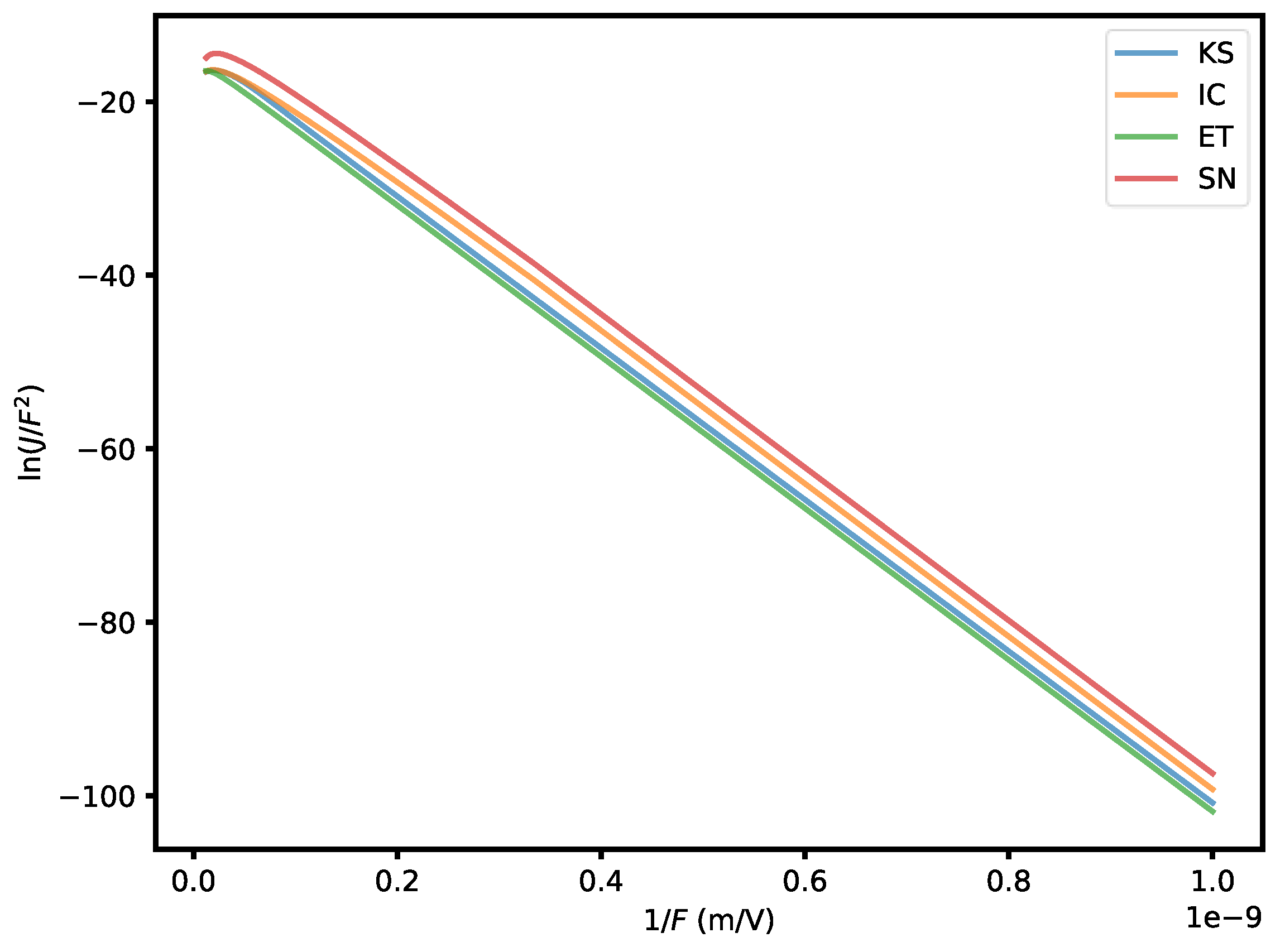
Finally, we present the emission current densities as a function of the applied electric field, using the well-known Fowler-Nordheim plot (Figure 5). For an ET potential, the analytical solution on this plot is a straight line with negative slope. Our results show this behavior for all four potentials, for fields less than 10 GV/m. The slopes of all curves are comparable in this region, so our new potentials (KS and IC) would not account for the experimentally deduced field enhancement factor that tends to increase these slopes [27]. For fields greater than 10 GV/m, all four curves are concave down, indicating that the emission current densities are smaller than expected. This is most likely due to the overprediction by the first-order Taylor expansion in the FN framework (Figure 4).
The difference in emission current densities among the four potentials is most pronounced at low electric fields. The SN potential has the greatest predicted emission current densities, followed by the IC, KS, and ET potentials. This hierarchy is also the order of barrier heights from lowest to greatest as would be expected.
4. Discussion
This study is part of the continuing efforts to build accurate numerical models for field electron emission. We used a generalized FN framework for greater electric fields up to 80 GV/m and replaced the WKB approximation and the first-order Taylor expansion. The correction factors due to these two effects are presented. Except for the tunneling pre-factor to the ET potential, both correction factors are less than 1 for all potentials in the high field limit. We also obtain the KS and IC potentials from a DFT calculation, and these two potentials produce similar results despite the numerical artifact in the KS potential. The current framework can be employed to study different metal surfaces, including those with defects and adsorbates, as they can be partly modeled by DFT [28,29]. This study also has implications for laser field emission, which in the high field limit can be studied semi-classically using instantaneous tunneling currents.
Our numerical method, though, has several limitations. First, the source of the artifact in the one-dimensional KS potential is unclear. It can be examined by optimizing the lattice parameter or using a larger lattice in DFT, both of which are more computationally expensive. Second, the generation of the KS potential at fields above 1 GV/m assumes the electrical surface to be fixed. Although this seems true for fields up to 1 GV/m, this claim needs further examination in the high field limit. Finally, metallic surfaces cannot withstand a static field as large as 80 GV/m, which will necessarily lead to breakdown. Therefore, our results in the high-field limit should be regarded as applicable to transient perturbations only.
Our DFT-based field emission model can be further improved. We have not considered the band structure of a real metallic surface and instead used the free electron model, neither have we incorporated thermionic effects on the Fermi-Dirac distribution of electrons [26]. Incorporating these two effects would lead to a more complete one-dimensional model of field electron emission. We are well-situated for generalization to a three-dimensional model since the KS potentials are given on a three-dimensional grid. Such a calculation may be helpful in determining the effects of transverse momentum on emission, which could have implications on emitted beam quality in electron sources such as nanoblades. To evaluate this system, one possible solution is to use the three-dimensional TM method to calculate the transmission coefficient [25]. From there, we can then additionally incorporate surface effects such as defects and adsorbates into our field electron emission model.
Author Contributions
Conceptualization, Yiming Li, Joshua Mann; methodology, Yiming Li; software, Yiming Li; validation, Yiming Li; formal analysis, Yiming Li, Joshua Mann; investigation, Yiming Li; resources, Joshua Mann, James Rosenzweig; data curation, Yiming Li; writing—original draft preparation, Yiming Li; writing—review and editing, Joshua Mann, James Rosenzweig; visualization, Yiming Li; supervision, James Rosenzweig; project administration, James Rosenzweig; funding acquisition, James Rosenzweig. All authors have read and agreed to the published version of the manuscript.
Funding
This research was funded by the Center for Bright Beams, National Science Foundation Grant No. PHY-1549132.
Data Availability Statement
The code can be found at https://github.com/yimingli57/field_electron_emission.git. The DFT results can be obtained from the corresponding author upon reasonable request.
Conflicts of Interest
The authors declare no conflict of interest.
Appendix A
According to the free electron assumption, the electrons are evenly distributed in total energy and normal energy below the Fermi level. The emission current density takes the form , where is the surface-parallel kinetic energy and the electron total energy [5]. In our calculation, the transmission coefficient is only a function of electron normal energy , so we use change of variables to convert the integral. The complete integral can be written as
By conservation of energy, , so we can change the inner integral from to :
Now reverse the order of integration:
The inner integral over no longer explicitly depends on , so it can be performed directly. The final result is
References
- Wuensch, W. High-Gradient Breakdown in Normal-Conducting RF Cavities. Proc 8th Eup Part Accel Conf 2002, 134. [Google Scholar]
- Lawler G, Majernik N, Mann J, Montanez N, Rosenzweig J, Yu V. Emittance Measurements of Nanoblade-Enhanced High Field Cathode. Proc 13th Int Part Accel Conf 2022.
- Mann J, Arias T, Karkare S, Lawler G, Nangoi JK, Rosenzweig J, et al. Simulations of Nanoblade Cathode Emissions with Image Charge Trapping for Yield and Brightness Analyses. Proc 5th North American Part Accel Conf 2022. [Google Scholar]
- Keldysh, LV. IONIZATION IN THE FIELD OF A STRONG ELECTROMAGNETIC WAVE. Zh Eksperim Teor Fiz 1964, 47. [Google Scholar]
- Forbes RG. Use of energy-space diagrams in free-electron models of field electron emission. Surf Interface Anal 2004, 36, 395–401. [CrossRef]
- Nordhiem LW, Fowler RH. The effect of the image force on the emission and reflexion of electrons by metals. Proc R Soc Lond Ser Contain Pap Math Phys Character 1997, 121, 626–639. [Google Scholar]
- Mayer, A. Exact solutions for the field electron emission achieved from a flat metal using the standard Fowler–Nordheim equation with a correction factor that accounts for the electric field, the work function, and the Fermi energy of the emitter. J Vac Sci Technol B 2011, 29, 021803. [Google Scholar] [CrossRef]
- Lawler GE, Mann J, Yu V, Rosenzweig JB, Roussel R. Initial Nanoblade-Enhanced Laser-Induced Cathode Emission Measurements. Proc 12th Int Part Accel Conf. 2021.
- Sundararaman R, Letchworth-Weaver K, Schwarz KA, Gunceler D, Ozhabes Y, Arias TA. JDFTx: Software for joint density-functional theory. SoftwareX 2017, 6, 278–284. [Google Scholar] [CrossRef]
- Jalili S, Isfahani AZ, Habibpour R. DFT investigations on the interaction of oxygen reduction reaction intermediates with Au (100) and bimetallic Au/M (100) (M=Pt, Cu, and Fe) surfaces. Int J Ind Chem 2013, 4, 1–12. [Google Scholar]
- Rumble, John. CRC Handbook of Chemistry and Physics, 102nd ed.; CRC Press: Boca Raton, USA, 2021. [Google Scholar]
- Garrity KF, Bennett JW, Rabe KM, Vanderbilt D. Pseudopotentials for high-throughput DFT calculations. Comput Mater Sci. 2014, 81, 446–452. [Google Scholar] [CrossRef]
- Schlipf M, Gygi F. Optimization algorithm for the generation of ONCV pseudopotentials. Comput Phys Commun 2015, 196, 36–44. [Google Scholar] [CrossRef]
- Plöger J, Mueller J, Jacob T, Anton J. Theoretical Studies on the Adsorption of 1-Butyl-3-methyl-imidazolium-hexafluorophosphate (BMI/PF6) on Au(100) Surfaces. Top Catal 2016, 59, 792–801. [CrossRef]
- Perdew JP, Chevary JA, Vosko SH, Jackson KA, Pederson MR, Singh DJ, et al. Atoms, molecules, solids, and surfaces: Applications of the generalized gradient approximation for exchange and correlation. Phys Rev B 1992, 46, 6671–6687. [Google Scholar] [CrossRef]
- Perdew JP, Burke K, Ernzerhof M. Generalized Gradient Approximation Made Simple. Phys Rev Lett 1996, 77, 3865–3868. [Google Scholar] [CrossRef]
- Sundararaman R, Arias TA. Regularization of the Coulomb singularity in exact exchange by Wigner-Seitz truncated interactions: Towards chemical accuracy in nontrivial systems. Phys Rev B 2013, 87, 165122. [Google Scholar] [CrossRef]
- Freysoldt C, Boeck S, Neugebauer J. Direct minimization technique for metals in density functional theory. Phys Rev B 2009, 79, 241103. [Google Scholar] [CrossRef]
- Sundararaman R, Ping Y. First-principles electrostatic potentials for reliable alignment at interfaces and defects. J Chem Phys 2017, 146, 104109. [Google Scholar] [CrossRef]
- Lepetit, B. Electronic field emission models beyond the Fowler-Nordheim one. J Appl Phys 2017, 122, 215105. [Google Scholar] [CrossRef]
- Forbes, RG. Calculation of the electrical-surface (image-plane) position for aluminium. Ultramicroscopy 1998, 73, 31–35. [Google Scholar] [CrossRef]
- Forbes, RG. The electrical surface as centroid of the surface-induced charge. Ultramicroscopy 1999, 79, 25–34. [Google Scholar] [CrossRef]
- Hairer E, Wanner G, Nørsett SP, editors. Runge-Kutta and Extrapolation Methods. In Solving Ordinary Differential Equations I: Nonstiff Problems. Springer: Berlin, Heidelberg, 1993; pp. 129–353.
- Forbes, RG. On the need for a tunneling pre-factor in Fowler–Nordheim tunneling theory. J Appl Phys 2008, 103, 114911. [Google Scholar] [CrossRef]
- Mayer, A. A comparative study of the electron transmission through one-dimensional barriers relevant to field-emission problems. J Phys Condens Matter 2010, 22, 175007. [Google Scholar] [CrossRef] [PubMed]
- Forbes, RG. Physics of generalized Fowler-Nordheim-type equations. J Vac Sci Technol B Microelectron Nanometer Struct 2008, 26, 788. [Google Scholar] [CrossRef]
- Schwettman HA, Turneaure JP, Waites RF. Evidence for surface-state-enhanced field emission in rf superconducting cavities. J Appl Phys 1974, 45, 914–922. [Google Scholar] [CrossRef]
- Lepetit, B. A three dimensional numerical quantum mechanical model of electronic field emission from metallic surfaces with nanoscale corrugation. J Appl Phys 2019, 125, 025107. [Google Scholar] [CrossRef]
- Márquez-Mijares M, Lepetit B. A three dimensional numerical quantum mechanical model of field electron emission from metallic surfaces covered with carbon adsorbates. J Appl Phys 2019, 126, 065107. [Google Scholar] [CrossRef]
Figure 1.
The one-dimensional KS, IC, ET, and SN potentials at zero electric field, from the center of the slab to the center of the vacuum.
Figure 1.
The one-dimensional KS, IC, ET, and SN potentials at zero electric field, from the center of the slab to the center of the vacuum.
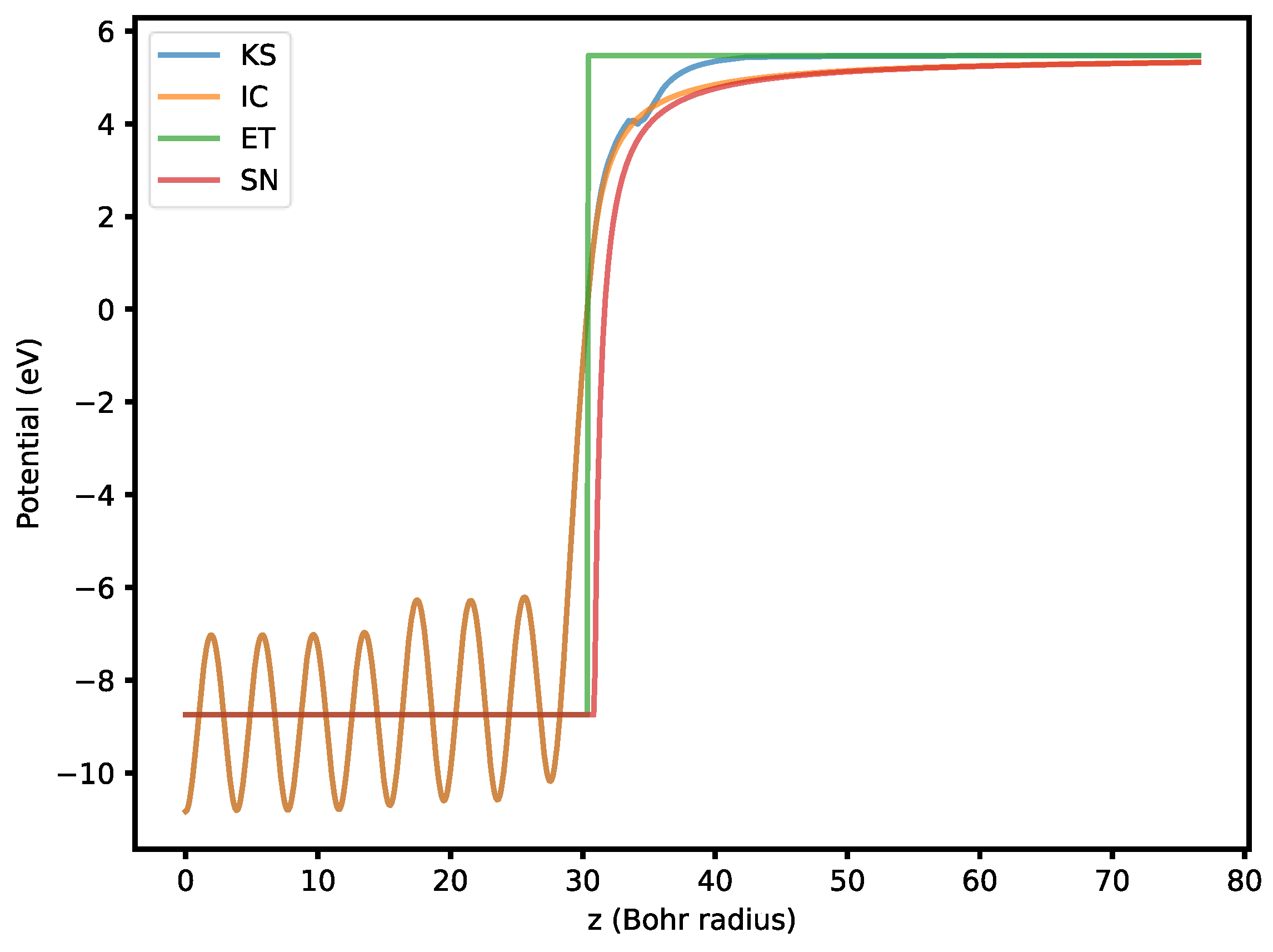
Figure 2.
Ratio of TM transmission coefficient to that of DOP853 for all surface potentials under consideration.
Figure 2.
Ratio of TM transmission coefficient to that of DOP853 for all surface potentials under consideration.
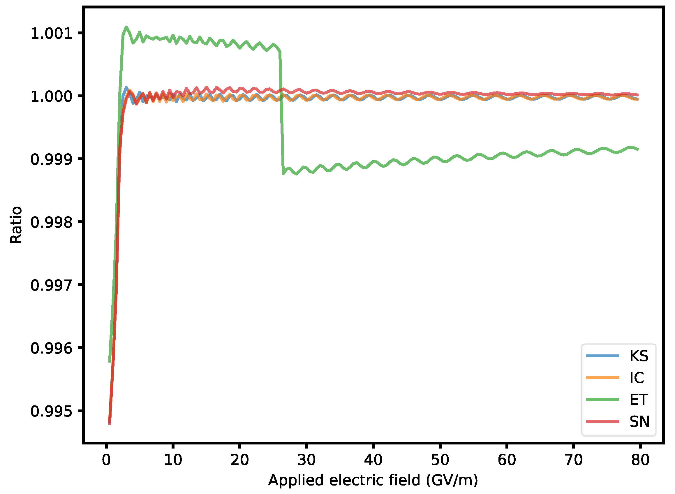
Figure 3.
Tunneling pre-factor to the WKB transmission coefficients.
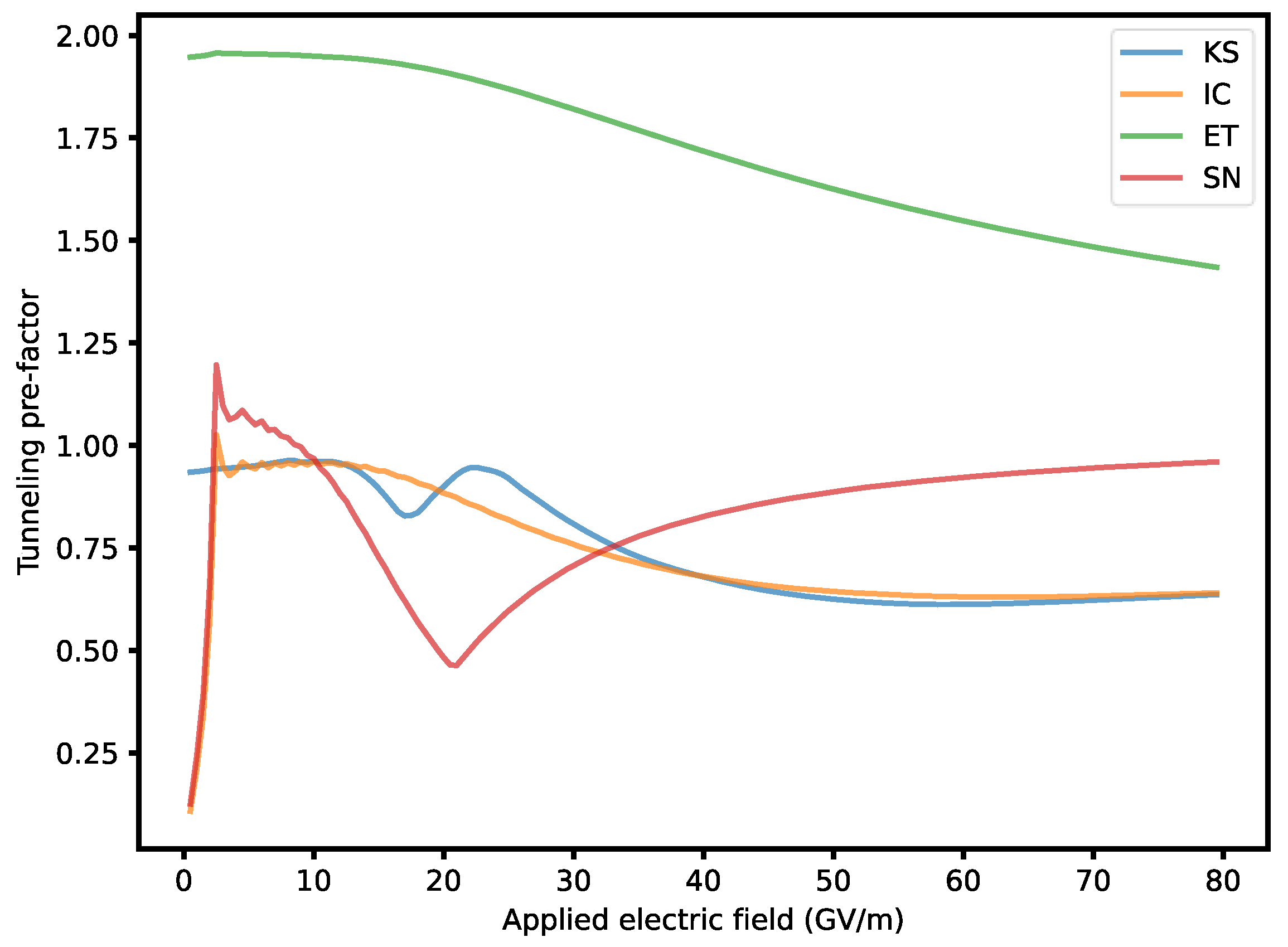
Figure 4.
Correction factor arising from the first-order Taylor expansion.

Figure 5.
Fowler-Nordheim plot of four potentials. denotes the applied electric field and the emission current density. The horizontal axis is the inverse of the applied electric field. The vertical axis is on a logarithmic scale.
Figure 5.
Fowler-Nordheim plot of four potentials. denotes the applied electric field and the emission current density. The horizontal axis is the inverse of the applied electric field. The vertical axis is on a logarithmic scale.
Disclaimer/Publisher’s Note: The statements, opinions and data contained in all publications are solely those of the individual author(s) and contributor(s) and not of MDPI and/or the editor(s). MDPI and/or the editor(s) disclaim responsibility for any injury to people or property resulting from any ideas, methods, instructions or products referred to in the content. |
© 2023 by the authors. Licensee MDPI, Basel, Switzerland. This article is an open access article distributed under the terms and conditions of the Creative Commons Attribution (CC BY) license (http://creativecommons.org/licenses/by/4.0/).
Copyright: This open access article is published under a Creative Commons CC BY 4.0 license, which permit the free download, distribution, and reuse, provided that the author and preprint are cited in any reuse.


